Barrier Frank-Wolfe for Marginal Inference

Abstract

We introduce a globally-convergent algorithm for optimizing the tree-reweighted (TRW) variational objective over the marginal polytope. The algorithm is based on the conditional gradient method (Frank-Wolfe) and moves pseudomarginals within the marginal polytope through repeated maximum a posteriori (MAP) calls. This modular structure enables us to leverage black-box MAP solvers (both exact and approximate) for variational inference, and obtains more accurate results than tree-reweighted algorithms that optimize over the local consistency relaxation. Theoretically, we bound the sub-optimality for the proposed algorithm despite the TRW objective having unbounded gradients at the boundary of the marginal polytope. Empirically, we demonstrate the increased quality of results found by tightening the relaxation over the marginal polytope as well as the spanning tree polytope on synthetic and real-world instances.

1 Introduction

Markov random fields (MRFs) are used in many areas of computer science such as vision and speech. Inference in these undirected graphical models is generally intractable. Our work focuses on performing approximate marginal inference by optimizing the Tree Re-Weighted (TRW) objective (Wainwright et al., 2005). The TRW objective is concave, is exact for tree-structured MRFs, and provides an upper bound on the log-partition function.

Fast combinatorial solvers for the TRW objective exist, including Tree-Reweighted Belief Propagation (TRBP) (Wainwright et al., 2005), convergent message-passing based on geometric programming (Globerson and Jaakkola, 2007), and dual decomposition (Jancsary and Matz, 2011). These methods optimize over the set of pairwise consistency constraints, also called the local polytope. Sontag and Jaakkola (2007) showed that significantly better results could be obtained by optimizing over tighter relaxations of the marginal polytope. However, deriving a message-passing algorithm for the TRW objective over tighter relaxations of the marginal polytope is challenging. Instead, Sontag and Jaakkola (2007) use the conditional gradient method (also called Frank-Wolfe) and off-the-shelf linear programming solvers to optimize TRW over the cycle consistency relaxation. Rather than optimizing over the cycle relaxation, Belanger et al. (2013) optimize the TRW objective over the exact marginal polytope. Then, using Frank-Wolfe, the linear minimization performed in the inner loop can be shown to correspond to MAP inference.

The Frank-Wolfe optimization algorithm has seen increasing use in machine learning, thanks in part to its efficient handling of complex constraint sets appearing with structured data (Jaggi, 2013; Lacoste-Julien and Jaggi, 2015). However, applying Frank-Wolfe to variational inference presents challenges that were never resolved in previous work. First, the linear minimization performed in the inner loop is computationally expensive, either requiring repeatedly solving a large linear program, as in Sontag and Jaakkola (2007), or performing MAP inference, as in Belanger et al. (2013). Second, the TRW objective involves entropy terms whose gradients go to infinity near the boundary of the feasible set, therefore existing convergence guarantees for Frank-Wolfe do not apply. Third, variational inference using TRW involves both an outer and inner loop of Frank-Wolfe, where the outer loop optimizes the edge appearance probabilities in the TRW entropy bound to tighten it. Neither Sontag and Jaakkola (2007) nor Belanger et al. (2013) explore the effect of optimizing over the edge appearance probabilities.

Although MAP inference is in general NP hard (Shimony, 1994), it is often possible to find exact solutions to large real-world instances within reasonable running times (Sontag et al., 2008; Allouche et al., 2010; Kappes et al., 2013). Moreover, as we show in our experiments, even approximate MAP solvers can be successfully used within our variational inference algorithm. As MAP solvers improve in their runtime and performance, their iterative use could become feasible and as a byproduct enable more efficient and accurate marginal inference. Our work provides a fast deterministic alternative to recently proposed Perturb-and-MAP algorithms (Papandreou and Yuille, 2011; Hazan and Jaakkola, 2012; Ermon et al., 2013).

Contributions. This paper makes several theoretical and practical innovations. We propose a modification to the Frank-Wolfe algorithm that optimizes over adaptively chosen contractions of the domain and prove its rate of convergence for functions whose gradients can be unbounded at the boundary. Our algorithm does not require a different oracle than standard Frank-Wolfe and could be useful for other convex optimization problems where the gradient is ill-behaved at the boundary.

We instantiate the algorithm for approximate marginal inference over the marginal polytope with the TRW objective. With an exact MAP oracle, we obtain the first provably convergent algorithm for the optimization of the TRW objective over the marginal polytope, which had remained an open problem to the best of our knowledge. Traditional proof techniques of convergence for first order methods fail as the gradient of the TRW objective is not Lipschitz continuous.

We develop several heuristics to make the algorithm practical: a fully-corrective variant of Frank-Wolfe that reuses previously found integer assignments thereby reducing the need for new (approximate) MAP calls, the use of local search between MAP calls, and significant re-use of computations between subsequent steps of optimizing over the spanning tree polytope. We perform an extensive experimental evaluation on both synthetic and real-world inference tasks.

2 Background

Markov Random Fields: MRFs are undirected probabilistic graphical models where the probability distribution factorizes over cliques in the graph. We consider marginal inference on pairwise MRFs with $N$ random variables $X_{1},X_{2},\ldots,X_{N}$ where each variable takes discrete states $x_{i}\in\textrm{VAL}_{i}$. Let $G=(V,E)$ be the Markov network with an undirected edge $\{i,j\}\in E$ for every two variables $X_{i}$ and $X_{j}$ that are connected together. Let $\mathcal{N}(i)$ refer to the set of neighbors of variable $X_{i}$. We organize the edge log-potentials $\theta_{ij}(x_{i},x_{j})$ for all possible values of $x_{i}\in\textrm{VAL}_{i}$, $x_{j}\in\textrm{VAL}_{j}$ in the vector $\bm{\theta}_{ij}$, and similarly for the node log-potential vector $\bm{\theta}_{i}$. We regroup these in the overall vector $\vec{\bm{\theta}}$. We introduce a similar grouping for the marginal vector $\vec{\bm{\mu}}$: for example, $\mu_{i}(x_{i})$ gives the coordinate of the marginal vector corresponding to the assignment $x_{i}$ to variable $X_{i}$.

Tree Re-weighted Objective (Wainwright et al., 2005): Let $Z(\vec{\bm{\theta}})$ be the partition function for the MRF and $\mathcal{M}$ be the set of all valid marginal vectors (the marginal polytope). The maximization of the TRW objective gives the following upper bound on the log partition function:

$$\begin{split}\log Z(\vec{\bm{\theta}})&\leq\min_{\bm{\rho}\in\mathbb{T}}\max_{\vec{\bm{\mu}}\in\mathcal{M}}\quad\underbrace{\langle\vec{\bm{\theta}},\vec{\bm{\mu}}\rangle+H(\vec{\bm{\mu}};\bm{\rho})}_{\text{TRW}(\vec{\bm{\mu}};\vec{\bm{\theta}},\bm{\rho})},\end{split}$$ (1)

where the TRW entropy is:

$$H(\vec{\bm{\mu}};\bm{\rho}):=\sum_{i\in V}(1-\sum_{j\in\mathcal{N}(i)}\rho_{ij})H(\bm{\mu}_{i})+\sum_{(ij)\in E}\rho_{ij}H(\bm{\mu}_{ij}),\quad H(\bm{\mu}_{i}):=-\sum_{x_{i}}\mu_{i}(x_{i})\log\mu_{i}(x_{i}).$$ (2)

$\mathbb{T}$ is the spanning tree polytope, the convex hull of edge indicator vectors of all possible spanning trees of the graph. Elements of $\bm{\rho}\in\mathbb{T}$ specify the probability of an edge being present under a specific distribution over spanning trees. $\mathcal{M}$ is difficult to optimize over, and most TRW algorithms optimize over a relaxation called the local consistency polytope $\mathbb{L}\supseteq\mathcal{M}$:

The TRW objective $\text{TRW}(\vec{\bm{\mu}};\vec{\bm{\theta}},\bm{\rho})$ is a globally concave function of $\vec{\bm{\mu}}$ over $\mathbb{L}$, assuming that $\bm{\rho}$ is obtained from a valid distribution over spanning trees of the graph (i.e. $\bm{\rho}\in\mathbb{T}$).

Frank-Wolfe (FW) Algorithm: In recent years, the Frank-Wolfe (aka conditional gradient) algorithm has gained popularity in machine learning (Jaggi, 2013) for the optimization of convex functions over compact domains (denoted $\mathcal{D}$). The algorithm is used to solve $\min_{\bm{x}\in\mathcal{D}}f(\bm{x})$ by iteratively finding a good descent vertex by solving the linear subproblem:

$$\bm{s}^{(k)}=\operatorname*{\arg\min}_{\bm{s}\in\mathcal{D}}\langle\nabla f(\bm{x}^{(k)}),\bm{s}\rangle\qquad\text{(FW oracle)},$$ (3)

and then taking a convex step towards this vertex: $\bm{x}^{(k+1)}=(1-\gamma)\bm{x}^{(k)}+\gamma\bm{s}^{(k)}$ for a suitably chosen step-size $\gamma\in[0,1]$. The algorithm remains within the feasible set (is projection free), is invariant to affine transformations of the domain, and can be implemented in a memory efficient manner. Moreover, the FW gap $g(\bm{x}^{(k)}):=\langle-\nabla f(\bm{x}^{(k)}),\bm{s}^{(k)}-\bm{x}^{(k)}\rangle$ provides an upper bound on the suboptimality of the iterate $\bm{x}^{(k)}$. The primal convergence of the Frank-Wolfe algorithm is given by Thm. $1$ in Jaggi (2013), restated here for convenience: for $k\geq 1$, the iterates $\bm{x}^{(k)}$ satisfy:

$$f(\bm{x}^{(k)})-f(\bm{x}^{*})\leq\frac{2C_{f}}{k+2},$$ (4)

where $C_{f}$ is called the “curvature constant”. Under the assumption that $\nabla f$ is $L$-Lipschitz continuous on $\mathcal{D}$, we can bound it as $C_{f}\leq L\operatorname{diam}_{||.||}(\mathcal{D})^{2}$.

Marginal Inference with Frank-Wolfe: To optimize $\max_{\vec{\bm{\mu}}\in\mathcal{M}}\text{TRW}(\vec{\bm{\mu}};\vec{\bm{\theta}},\bm{\rho})$ with Frank-Wolfe, the linear subproblem (3) becomes $\operatorname*{\arg\max}_{\vec{\bm{\mu}}\in\mathcal{M}}\langle\tilde{\bm{\theta}},\vec{\bm{\mu}}\rangle$, where the perturbed potentials $\tilde{\bm{\theta}}$ correspond to the gradient of $\text{TRW}(\vec{\bm{\mu}};\vec{\bm{\theta}},\bm{\rho})$ with respect to $\vec{\bm{\mu}}$. Elements of $\tilde{\bm{\theta}}$ are of the form $\theta_{c}(x_{c})+K_{c}(1+\log\mu_{c}(x_{c}))$, evaluated at the pseudomarginals’ current location in $\mathcal{M}$, where $K_{c}$ is the coefficient of the entropy for the node/edge term in (2). The FW linear subproblem here is thus equivalent to performing MAP inference in a graphical model with potentials $\tilde{\bm{\theta}}$ (Belanger et al., 2013), as the vertices of the marginal polytope are in 1-1 correspondence with valid joint assignments to the random variables of the MRF, and the solution of a linear program is always achieved at a vertex of the polytope. The TRW objective does not have a Lipschitz continuous gradient over $\mathcal{M}$, and so standard convergence proofs for Frank-Wolfe do not hold.

3 Optimizing over Contractions of the Marginal Polytope

Motivation: We wish to (1) use the fewest possible MAP calls, and (2) avoid regions near the boundary where the unbounded curvature of the function slows down convergence. A viable option to address (1) is through the use of correction steps, where after a Frank-Wolfe step, one optimizes over the polytope defined by previously visited vertices of $\mathcal{M}$ (called the fully-corrective Frank-Wolfe (FCFW) algorithm and proven to be linearly convergence for strongly convex objectives (Lacoste-Julien and Jaggi, 2015)). This does not require additional MAP calls. However, we found (see Sec. 5) that when optimizing the TRW objective over $\mathcal{M}$, performing correction steps can surprisingly hurt performance. This leaves us in a dilemma: correction steps enable decreasing the objective without additional MAP calls, but they can also slow global progress since iterates after correction sometimes lie close to the boundary of the polytope (where the FW directions become less informative). In a manner akin to barrier methods and to Garber and Hazan (2013)’s local linear oracle, our proposed solution maintains the iterates within a contraction of the polytope. This gives us most of the mileage obtained from performing the correction steps without suffering the consequences of venturing too close to the boundary of the polytope. We prove a global convergence rate for the iterates with respect to the true solution over the full polytope.

We describe convergent algorithms to optimize $\text{TRW}(\vec{\bm{\mu}};\vec{\bm{\theta}},\bm{\rho})$ for $\vec{\bm{\mu}}\in\mathcal{M}$. The approach we adopt to deal with the issue of unbounded gradients at the boundary is to perform Frank-Wolfe within a contraction of the marginal polytope given by $\mathcal{M}_{\delta}$ for $\delta\in[0,1]$, with either a fixed $\delta$ or an adaptive $\delta$.

Definition 3.1 (Contraction polytope).

$\mathcal{M}_{\delta}:=(1-\delta)\mathcal{M}+\delta\,\bm{u}_{0}$, where $\bm{u}_{0}\in\mathcal{M}$ is the vector representing the uniform distribution.

Marginal vectors that lie within $\mathcal{M}_{\delta}$ are bounded away from zero as all the components of $\bm{u}_{0}$ are strictly positive. Denoting $\mathcal{V}^{(\delta)}$ as the set of vertices of $\mathcal{M}_{\delta}$, $\mathcal{V}$ as the set of vertices of $\mathcal{M}$ and $f(\vec{\bm{\mu}}):=-\text{TRW}(\vec{\bm{\mu}};\vec{\bm{\theta}},\bm{\rho})$, the key insight that enables our novel approach is that:

$$\underbrace{\operatorname*{\arg\min}_{\bm{v}^{(\delta)}\in\mathcal{V}^{(\delta)}}\left\langle\nabla f,\bm{v}^{(\delta)}\right\rangle}_{\quad\emph{{(Linear Minimization over $\mathcal{M}_{\delta}$)}}}\equiv\operatorname*{\arg\min}_{\bm{v}\in\mathcal{V}}\underbrace{\left\langle\nabla f,(1-\delta)\bm{v}+\delta\bm{u}_{0}\right\rangle}_{\quad\emph{{(Definition of $\bm{v}^{(\delta)}$)}}}\equiv\underbrace{(1-\delta)\operatorname*{\arg\min}_{\bm{v}\in\mathcal{V}}\left\langle\nabla f,\bm{v}\right\rangle+\delta\bm{u}_{0}.}_{\quad\emph{{(Run MAP solver and shift vertex)}}}$$

Therefore, to solve the FW subproblem (3) over $\mathcal{M}_{\delta}$, we can run as usual a MAP solver and simply shift the resulting vertex of $\mathcal{M}$ towards $\bm{u}_{0}$ to obtain a vertex of $\mathcal{M}_{\delta}$. Our solution to optimize over restrictions of the polytope is more broadly applicable to the optimization problem defined below, with $f$ satisfying Prop. 3.3 (satisfied by the TRW objective) in order to get convergence rates.

Problem 3.2.

Solve $\min_{\bm{x}\in\mathcal{D}}f(\bm{x})$ where $\mathcal{D}$ is a compact convex set and $f$ is convex and continuously differentiable on the relative interior of $\mathcal{D}$.

Property 3.3.

(Controlled growth of Lipschitz constant over $\mathcal{D}_{\delta}$). We define $\mathcal{D}_{\delta}:=(1-\delta)\mathcal{D}+\delta\bm{u}_{0}$ for a fixed $\bm{u}_{0}$ in the relative interior of $\mathcal{D}$. We suppose that there exists a fixed $p\geq 0$ and $L$ such that for any $\delta>0$, $\nabla f(\bm{x})$ has a bounded Lipschitz constant $L_{\delta}\leq L\delta^{-p}\,\,\,\forall\bm{x}\in\mathcal{D}_{\delta}$.

Fixed $\delta$: The first algorithm fixes a value for $\delta$ a-priori and performs the optimization over $\mathcal{D}_{\delta}$. The following theorem bounds the sub-optimality of the iterates with respect to the optimum over $\mathcal{D}$.

Theorem 3.4 (Suboptimality bound for fixed-$\delta$ algorithm).

Let $f$ satisfy the properties in Prob. 3.2 and Prop. 3.3, and suppose further that $f$ is finite on the boundary of $\mathcal{D}$. Then the use of Frank-Wolfe for $\min_{\bm{x}\in\mathcal{D}_{\delta}}f(\bm{x})$ realizes a sub-optimality over $\mathcal{D}$ bounded as:

$$f(\bm{x}^{(k)})-f(\bm{x}^{*})\leq\frac{2C_{\delta}}{(k+2)}+\omega\left(\delta\operatorname{diam}(\mathcal{D})\right),$$

where $\bm{x}^{*}$ is the optimal solution in $\mathcal{D}$, $C_{\delta}\leq L_{\delta}\operatorname{diam}_{||.||}(\mathcal{D}_{\delta})^{2}$, and $\omega$ is the modulus of continuity function of the (uniformly) continuous $f$ (in particular, $\omega(\delta)\downarrow 0$ as $\delta\downarrow 0$).

The full proof is given in App. C. The first term of the bound comes from the standard Frank-Wolfe convergence analysis of the sub-optimality of $\bm{x}^{(k)}$ relative to $\bm{x}^{*}_{(\delta)}$, the optimum over $\mathcal{D}_{\delta}$, as in (4) and using Prop. 3.3. The second term arises by bounding $f(\bm{x}^{*}_{(\delta)})-f(\bm{x}^{*})\leq f(\tilde{\bm{x}})-f(\bm{x}^{*})$ with a cleverly chosen $\tilde{\bm{x}}\in\mathcal{D}_{\delta}$ (as $\bm{x}^{*}_{(\delta)}$ is optimal in $\mathcal{D}_{\delta}$). We pick $\tilde{\bm{x}}:=(1-\delta)\bm{x}^{*}+\delta\bm{u}_{0}$ and note that $\|\tilde{\bm{x}}-\bm{x}^{*}\|\leq\delta\operatorname{diam}(\mathcal{D})$. As $f$ is continuous on a compact set, it is uniformly continuous and we thus have $f(\tilde{\bm{x}})-f(\bm{x}^{*})\leq\omega(\delta\operatorname{diam}(\mathcal{D}))$ with $\omega$ its modulus of continuity function.

Adaptive $\delta$: The second variant to solve $\min_{\bm{x}\in\mathcal{D}}f(\bm{x})$ iteratively perform FW steps over $\mathcal{D}_{\delta}$, but also decreases $\delta$ adaptively. The update schedule for $\delta$ is given in Alg. 1 and is motivated by the convergence proof. The idea is to ensure that the FW gap over $\mathcal{D}_{\delta}$ is always at least half the FW gap over $\mathcal{D}$, relating the progress over $\mathcal{D}_{\delta}$ with the one over $\mathcal{D}$. It turns out that $\text{FW-gap-}\mathcal{D}_{\delta}=(1-\delta)\text{FW-gap-}\mathcal{D}+\delta\cdot g_{u}(\bm{x}^{(k)})$, where the “uniform gap” $g_{u}(\bm{x}^{(k)})$ quantifies the decrease of the function when contracting towards $\bm{u}_{0}$. When $g_{u}(\bm{x}^{(k)})$ is negative and large compared to the FW gap, we need to shrink $\delta$ (see step 5 in Alg. 1) to ensure that the $\delta$-modified direction is a sufficient descent direction.

1:  At iteration $k$. Assuming $\bm{x}^{(k)},\bm{u}_{0},\delta^{(k-1)},f$ are defined and $\bm{s}^{(k)}$ has been computed

2:  Compute $g(\bm{x}^{(k)})=\langle-\nabla f(\bm{x}^{(k)}),\bm{s}^{(k)}-\bm{x}^{(k)}\rangle$  (Compute FW gap)

3:  Compute $g_{u}(\bm{x}^{(k)})=\langle-\nabla f(\bm{x}^{(k)}),\bm{u}_{0}-\bm{x}^{(k)}\rangle$  (Compute “uniform gap”)

4:  if $g_{u}(\bm{x}^{(k)})<0$ then

5:     Let $\tilde{\delta}=\frac{g(\bm{x}^{(k)})}{-4g_{u}(\bm{x}^{(k)})}$  (Compute new proposal for $\delta$)

6:     if $\tilde{\delta}<\delta^{(k-1)}$ then

7:        $\delta^{(k)}=\min\left(\tilde{\delta},\frac{\delta^{(k-1)}}{2}\right)$  (Shrink by at least a factor of two if proposal is smaller)

8:     end if

9:  end if (and set $\delta^{(k)}=\delta^{(k-1)}$ if it was not updated)

Algorithm 1 Updates to $\delta$ after a MAP call (Adaptive $\delta$ variant)

We can show that the algorithm converges to the global solution as follows:

Theorem 3.5 (Global convergence for adaptive-$\delta$ variant over $\mathcal{D}$).

For a function $f$ satisfying the properties in Prob. 3.2 and Prop. 3.3, the sub-optimality of the iterates obtained by running the FW updates over $\mathcal{D}_{\delta}$ with $\delta$ updated according to Alg. 1 is bounded as:

$$f(\bm{x}^{(k)})-f(\bm{x}^{*})\leq O\left(k^{-\frac{1}{p+1}}\right).$$

A full proof with a precise rate and constants is given in App. D. The sub-optimality $h_{k}:=f(\bm{x}^{(k)})-f(\bm{x}^{*})$ traverses three stages with an overall rate as above. The updates to $\delta^{(k)}$ as in Alg. 1 enable us to (1) upper bound the duality gap over $\mathcal{D}$ as a function of the duality gap in $\mathcal{D}_{\delta}$ and (2) lower bound the value of $\delta^{(k)}$ as a function of $h_{k}$. Applying the standard Descent Lemma with the Lipschitz constant on the gradient of the form $L\delta^{-p}$ (Prop. 3.3), and replacing $\delta^{(k)}$ by its bound in $h_{k}$, we get the recurrence: $h_{k+1}\leq h_{k}-Ch_{k}^{p+2}$. Solving this gives us the desired bound.

Application to the TRW Objective: $\min_{\vec{\bm{\mu}}\in\mathcal{M}}-\text{TRW}(\vec{\bm{\mu}};\vec{\bm{\theta}},\bm{\rho})$ is akin to $\min_{\bm{x}\in\mathcal{D}}f(\bm{x})$ and the (strong) convexity of $-\text{TRW}(\vec{\bm{\mu}};\vec{\bm{\theta}},\bm{\rho})$ has been previously shown (Wainwright et al., 2005; London et al., 2015). The gradient of the TRW objective is Lipschitz continuous over $\mathcal{M}_{\delta}$ since all marginals are strictly positive. Its growth for Prop. 3.3 can be bounded with $p=1$ as we show in App. E.1. This gives a rate of convergence of $O(k^{-1/2})$ for the adaptive-$\delta$ variant, which interestingly is a typical rate for non-smooth convex optimization. The hidden constant is of the order $O(\|\theta\|\cdot|V|)$. The modulus of continuity $\omega$ for the TRW objective is close to linear (it is almost a Lipschitz function), and its constant is instead of the order $O(\|\theta\|+|V|)$.

4 Algorithm

Alg. 2 describes the pseudocode for our proposed algorithm to do marginal inference with $\text{TRW}(\vec{\bm{\mu}};\vec{\bm{\theta}},\bm{\rho})$. minSpanTree finds the minimum spanning tree of a weighted graph, and $\textbf{{edgesMI}}(\vec{\bm{\mu}})$ computes the mutual information of edges of $G$ from the pseudomarginals in $\vec{\bm{\mu}}$ (to perform FW updates over $\bm{\rho}$ as in Alg. 2 in Wainwright et al. (2005)). It is worthwhile to note that our approach uses three levels of Frank-Wolfe: (1) for the (tightening) optimization of $\bm{\rho}$ over $\mathbb{T}$, (2) to perform approximate marginal inference, i.e for the optimization of $\vec{\bm{\mu}}$ over $\mathcal{M}$, and (3) to perform the correction steps (lines 16 and 23).

1:  Function TRW-Barrier-FW$(\bm{\rho}^{(0)},\epsilon,\delta^{(\mathrm{init})},\bm{u}_{0})$:

2:  Inputs: Edge-appearance probabilities $\bm{\rho}^{(0)}$, $\delta^{(\mathrm{init})}\leq\frac{1}{4}$ initial contraction of polytope, inner loop stopping criterion $\epsilon$, fixed reference point $\bm{u}_{0}$ in the interior of $\mathcal{M}$. Let $\delta^{(-1)}=\delta^{(\mathrm{init})}$.

3:  Let $V:=\{\bm{u}_{0}\}$ (visited vertices), $\bm{x}^{(0)}=\bm{u}_{0}$  (Initialize the algorithm at the uniform distribution)

4:  for $i=0\dots\textbf{{MAX$\_$RHO$\_$ITS}}$ do {FW outer loop to optimize $\bm{\rho}$ over $\mathbb{T}$}

5:     for $k=0\dots\textbf{{MAXITS}}$ do {FCFW inner loop to optimize $\bm{x}$ over $\mathcal{M}$}

6:        Let $\tilde{\theta}=\nabla f(\bm{x}^{(k)};\vec{\bm{\theta}},\bm{\rho}^{(i)})$  (Compute gradient)

7:        Let $\bm{s}^{(k)}\in\displaystyle\operatorname*{\arg\min}_{\bm{v}\in\mathcal{M}}\,\,\langle\tilde{\theta},\bm{v}\rangle$  (Run MAP solver to compute FW vertex)

8:        Compute $g(\bm{x}^{(k)})=\langle-\tilde{\theta},\bm{s}^{(k)}-\bm{x}^{(k)}\rangle$  (Inner loop FW duality gap)

9:        if $g(\bm{x}^{(k)})\leq\epsilon$ then

10:           break FCFW inner loop  ($\bm{x}^{(k)}$ is $\epsilon$-optimal)

11:        end if

12:        $\delta^{(k)}=\delta^{(k-1)}$  (For Adaptive-$\delta$: Run Alg. 1 to modify $\delta$)

13:        Let $\bm{s}^{(k)}_{(\delta)}=(1-\delta^{(k)})\bm{s}^{(k)}+\delta^{(k)}\bm{u}_{0}$ and $\bm{d}^{(k)}_{(\delta)}=\bm{s}^{(k)}_{(\delta)}-\bm{x}^{(k)}$  ($\delta$-contracted quantities)

14:        $\bm{x}^{(k+1)}=\arg\min\{f(\bm{x}^{(k)}+\gamma\,\bm{d}^{(k)}_{(\delta)}):\gamma\in[0,1]\}$  (FW step with line search)

15:        Update correction polytope: $V:=V\cup\{\bm{s}^{(k)}\}$

16:        $\bm{x}^{(k+1)}:=\textbf{{CORRECTION}}(\bm{x}^{(k+1)},V,\delta^{(k)},\bm{\rho}^{(i)})$  (optional: correction step)

17:        $\bm{x}^{(k+1)},V_{\mathrm{search}}:=\textbf{{LOCALSEARCH}}(\bm{x}^{(k+1)},\bm{s}^{(k)},\delta^{(k)},\bm{\rho}^{(i)})$  (optional: fast MAP solver)

18:        Update correction polytope (with vertices from LOCALSEARCH): $V:=V\cup\{V_{\mathrm{search}}\}$

19:     end for

20:     $\bm{\rho}^{v}\leftarrow\textrm{{minSpanTree}}(\textbf{{edgesMI}}(\bm{x}^{(k)}))$  (FW vertex of the spanning tree polytope)

21:     $\bm{\rho}^{(i+1)}\leftarrow\bm{\rho}^{(i)}+(\frac{i}{i+2})(\bm{\rho}^{v}-\bm{\rho}^{(i)})$  (Fixed step-size schedule FW update for $\bm{\rho}$ kept in $\mathrm{relint}(\mathbb{T}$))

22:     $\bm{x}^{(0)}\leftarrow\bm{x}^{(k)}$, $\quad\delta^{(-1)}\leftarrow\delta^{(k-1)}$  (Re-initialize for FCFW inner loop)

23:     If $i<\textbf{{MAX$\_$RHO$\_$ITS}}$ then $\bm{x}^{(0)}=\textbf{{CORRECTION}}(\bm{x}^{(0)},V,\delta^{(-1)},\bm{\rho}^{(i+1)})$

24:  end for

25:  return  $\bm{x}^{(0)}$ and $\bm{\rho}^{(i)}$

Algorithm 2 Approximate marginal inference over $\mathcal{M}$ (solving (1)). Here $f$ is the negative TRW objective.

We detail a few heuristics that aid practicality.

Fast Local Search: Fast methods for MAP inference such as Iterated Conditional Modes (Besag, 1986) offer a cheap, low cost alternative to a more expensive combinatorial MAP solver. We warm start the ICM solver with the last found vertex $\bm{s}^{(k)}$ of the marginal polytope. The subroutine LOCALSEARCH (Alg. 6 in Appendix) performs a fixed number of FW updates to the pseudomarginals using ICM as the (approximate) MAP solver.

Re-optimizing over the Vertices of $\mathcal{M}$ (FCFW algorithm): As the iterations of FW progress, we keep track of the vertices of the marginal polytope found by Alg. 2 in the set $V$. We make use of these vertices in the CORRECTION subroutine (Alg. 5 in Appendix) which re-optimizes the objective function over (a contraction of) the convex hull of the elements of $V$ (called the correction polytope). $\bm{x}^{(0)}$ in Alg. 2 is initialized to the uniform distribution which is guaranteed to be in $\mathcal{M}$ (and $\mathcal{M}_{\delta}$). After updating $\bm{\rho}$, we set $\bm{x}^{(0)}$ to the approximate minimizer in the correction polytope. The intuition is that changing $\bm{\rho}$ by a small amount may not substantially modify the optimal $\bm{x}^{*}$ (for the new $\bm{\rho}$) and that the new optimum might be in the convex hull of the vertices found thus far. If so, CORRECTION will be able to find it without resorting to any additional MAP calls. This encourages the MAP solver to search for new, unique vertices instead of rediscovering old ones.

Approximate MAP Solvers: We can swap out the exact MAP solver with an approximate MAP solver. The primal objective plus the (approximate) duality gap may no longer be an upper bound on the log-partition function (black-box MAP solvers could be considered to optimize over an inner bound to the marginal polytope). Furthermore, the gap over $\mathcal{D}$ may be negative if the approximate MAP solver fails to find a direction of descent. Since adaptive-$\delta$ requires that the gap be positive in Alg. 1, we take the max over the last gap obtained over the correction polytope (which is always non-negative) and the computed gap over $\mathcal{D}$ as a heuristic.

Theoretically, one could get similar convergence rates as in Thm. 3.4 and 3.5 using an approximate MAP solver that has a multiplicative guarantee on the gap (line 8 of Alg. 2), as was done previously for FW-like algorithms (see, e.g., Thm. C.1 in Lacoste-Julien et al. (2013)). With an $\epsilon$-additive error guarantee on the MAP solution, one can prove similar rates up to a suboptimality error of $\epsilon$. Even if the approximate MAP solver does not provide an approximation guarantee, if it returns an upper bound on the value of the MAP assignment (as do branch-and-cut solvers for integer linear programs, or Sontag et al. (2008)), one can use this to obtain an upper bound on $\log Z$ (see App. J).

5 Experimental Results

Setup: The L1 error in marginals is computed as: $\zeta_{\mu}:=\frac{1}{N}\sum_{i=1}^{N}|\mu_{i}(1)-\mu_{i}^{*}(1)|$. When using exact MAP inference, the error in $\log Z$ (denoted $\zeta_{\log Z}$) is computed by adding the duality gap to the primal (since this guarantees us an upper bound). For approximate MAP inference, we plot the primal objective. We use a non-uniform initialization of $\bm{\rho}$ computed with the Matrix Tree Theorem (Sontag and Jaakkola, 2007; Koo et al., 2007). We perform 10 updates to $\bm{\rho}$, optimize $\vec{\bm{\mu}}$ to a duality gap of $0.5$ on $\mathcal{M}$, and always perform correction steps. We use LOCALSEARCH only for the real-world instances. We use the implementation of TRBP and the Junction Tree Algorithm (to compute exact marginals) in libDAI (Mooij, 2010). Unless specified, we compute marginals by optimizing the TRW objective using the adaptive-$\delta$ variant of the algorithm (denoted in the figures as $M_{\delta})$.

MAP Solvers: For approximate MAP, we run three solvers in parallel: QPBO (Kolmogorov and Rother, 2007; Boykov and Kolmogorov, 2004), TRW-S (Kolmogorov, 2006) and ICM (Besag, 1986) using OpenGM (Andres et al., 2012) and use the result that realizes the highest energy. For exact inference, we use Gurobi Optimization (2015) or toulbar2 (Allouche et al., 2010).

Test Cases: All of our test cases are on binary pairwise MRFs. (1) Synthetic 10 nodes cliques: Same setup as Sontag and Jaakkola (2007, Fig. 2), with $9$ sets of $100$ instances each with coupling strength drawn from $\mathcal{U}[-\theta,\theta]$ for $\theta\in\{0.5,1,2,\ldots,8\}$. (2) Synthetic Grids: $15$ trials with $5\times 5$ grids. We sample $\theta_{i}\sim\mathcal{U}[-1,1]$ and $\theta_{ij}\in[-4,4]$ for nodes and edges. The potentials were $(-\theta_{i},\theta_{i})$ for nodes and $(\theta_{ij},-\theta_{ij};-\theta_{ij},\theta_{ij})$ for edges. (3) Restricted Boltzmann Machines (RBMs): From the Probabilistic Inference Challenge 2011. (4) Horses: Large ($N\approx 12000$) MRFs representing images from the Weizmann Horse Data (Borenstein and Ullman, 2002) with potentials learned by Domke (2013). (5) Chinese Characters: An image completion task from the KAIST Hanja2 database, compiled in OpenGM by Andres et al. (2012). The potentials were learned using Decision Tree Fields (Nowozin et al., 2011). The MRF is not a grid due to skip edges that tie nodes at various offsets. The potentials are a combination of submodular and supermodular and therefore a harder task for inference algorithms.

On the Optimization of $\mathcal{M}$ versus $\mathcal{M}_{\delta}$

We compare the performance of Alg. 2 on optimizing over $\mathcal{M}$ (with and without correction), optimizing over $\mathcal{M}_{\delta}$ with fixed-$\delta=0.0001$ (denoted $M_{0.0001}$) and optimizing over $\mathcal{M}_{\delta}$ using the adaptive-$\delta$ variant. These plots are averaged across all the trials for the first iteration of optimizing over $\mathbb{T}$. We show error as a function of the number of MAP calls since this is the bottleneck for large MRFs. Fig. 1(a), 1(b) depict the results of this optimization aggregated across trials. We find that all variants settle on the same average error. The adaptive $\delta$ variant converges faster on average followed by the fixed $\delta$ variant. Despite relatively quick convergence for $\mathcal{M}$ with no correction on the grids, we found that correction was crucial to reducing the number of MAP calls in subsequent steps of inference after updates to $\bm{\rho}$. As highlighted earlier, correction steps on $\mathcal{M}$ (in blue) worsen convergence, an effect brought about by iterates wandering too close to the boundary of $\mathcal{M}$.

On the Applicability of Approximate MAP Solvers

Synthetic Grids: Fig. 1(c) depicts the accuracy of approximate MAP solvers versus exact MAP solvers aggregated across trials for $5\times 5$ grids. The results using approximate MAP inference are competitive with those of exact inference, even as the optimization is tightened over $\mathbb{T}$. This is an encouraging and non-intuitive result since it indicates that one can achieve high quality marginals through the use of relatively cheaper approximate MAP oracles.

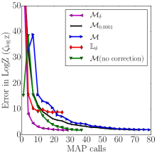
(a) $\zeta_{\log Z}$: $5\times 5$ grids   
$\mathcal{M}$ vs $\mathcal{M}_{\delta}$

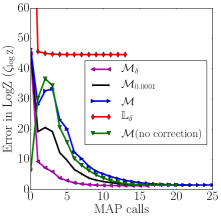
(b) $\zeta_{\log Z}$: $10$ node cliques   
$\mathcal{M}$ vs $\mathcal{M}_{\delta}$

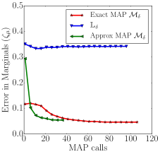
(c) $\zeta_{\mu}$: $5\times 5$ grids
Approx. vs. Exact MAP

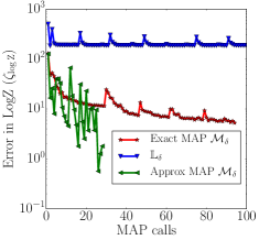
(d) $\zeta_{\log Z}$: 40 node RBM
Approx. vs. Exact MAP

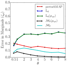
(e) $\zeta_{\mu}$: 10 node cliques
Optimization over $\mathbb{T}$

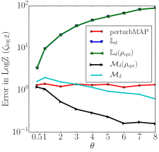
(f) $\zeta_{\log Z}$: 10 node cliques
Optimization over $\mathbb{T}$

Figure 1: Synthetic Experiments: In Fig. 1(c) & 1(d), we unravel MAP calls across updates to $\bm{\rho}$. Fig. 1(d) corresponds to a single RBM (not an aggregate over trials) where for “Approx MAP” we plot the absolute error between the primal objective and $\log Z$ (not guaranteed to be an upper bound).

RBMs: As in Salakhutdinov (2008), we observe for RBMs that the bound provided by $\text{TRW}(\vec{\bm{\mu}};\vec{\bm{\theta}},\bm{\rho})$ over $\mathbb{L}_{\delta}$ is loose and does not get better when optimizing over $\mathbb{T}$. As Fig. 1(d) depicts for a single RBM, optimizing over $\mathcal{M}_{\delta}$ realizes significant gains in the upper bound on $\log Z$ which improves with updates to $\bm{\rho}$. The gains are preserved with the use of the approximate MAP solvers. Note that there are also fast approximate MAP solvers specifically for RBMs (Wang et al., 2014).

Horses: See Fig. 2 (right). The models are close to submodular and the local relaxation is a good approximation to the marginal polytope. Our marginals are visually similar to those obtained by TRBP and our algorithm is able to scale to large instances by using approximate MAP solvers.

On the Importance of Optimizing over $\mathbb{T}$

Synthetic Cliques: In Fig. 1(e), 1(f), we study the effect of tightening over $\mathbb{T}$ against coupling strength $\theta$. We consider the $\zeta_{\mu}$ and $\zeta_{\log Z}$ obtained for the final marginals before updating $\bm{\rho}$ (step 19) and compare to the values obtained after optimizing over $\mathbb{T}$ (marked with $\bm{\rho}_{opt}$). The optimization over $\mathbb{T}$ has little effect on TRW optimized over $\mathbb{L}_{\delta}$. For optimization over $\mathcal{M}_{\delta}$, updating $\bm{\rho}$ realizes better marginals and bound on $\log Z$ (over and above those obtained in Sontag and Jaakkola (2007)).

Chinese Characters: Fig. 2 (left) displays marginals across iterations of optimizing over $\mathbb{T}$. The submodular and supermodular potentials lead to frustrated models for which $\mathbb{L}_{\delta}$ is very loose, which results in TRBP obtaining poor results. Our method produces reasonable marginals even before the first update to $\bm{\rho}$, and these improve with tightening over $\mathbb{T}$.

Related Work for Marginal Inference with MAP Calls

Hazan and Jaakkola (2012) estimate $\log Z$ by averaging MAP estimates obtained on randomly perturbed inflated graphs. Our implementation of the method performed well in approximating $\log Z$ but the marginals (estimated by fixing the value of each random variable and estimating $\log Z$ for the resulting graph) were less accurate than our method (Fig. 1(e), 1(f)).

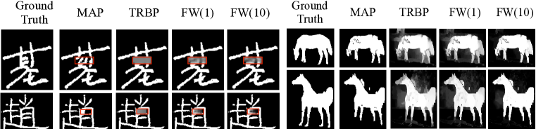
Figure 2: Results on real world test cases. FW(i) corresponds to the final marginals at the $i$th iteration of optimizing $\bm{\rho}$. The area highlighted on the Chinese Characters depicts the region of uncertainty.

6 Discussion

We introduce the first provably convergent algorithm for the TRW objective over the marginal polytope, under the assumption of exact MAP oracles. We quantify the gains obtained both from marginal inference over $\mathcal{M}$ and from tightening over the spanning tree polytope. We give heuristics that improve the scalability of Frank-Wolfe when used for marginal inference. The runtime cost of iterative MAP calls (a reasonable rule of thumb is to assume an approximate MAP call takes roughly the same time as a run of TRBP) is worthwhile particularly in cases such as the Chinese Characters where $\mathbb{L}$ is loose. Specifically, our algorithm is appropriate for domains where marginal inference is hard but there exist efficient MAP solvers capable of handling non-submodular potentials. Code is available at https://github.com/clinicalml/fw-inference.

Our work creates a flexible, modular framework for optimizing a broad class of variational objectives, not simply TRW, with guarantees of convergence. We hope that this will encourage more research on building better entropy approximations. The framework we adopt is more generally applicable to optimizing functions whose gradients tend to infinity at the boundary of the domain.

Our method to deal with gradients that diverge at the boundary bears resemblance to barrier functions used in interior point methods insofar as they bound the solution away from the constraints. Iteratively decreasing $\delta$ in our framework can be compared to decreasing the strength of the barrier, enabling the iterates to get closer to the facets of the polytope, although its worthwhile to note that we have an adaptive method of doing so.

Appendix A Preliminaries

A.1 Summary of Supplementary Material

The supplementary material is divided into two parts:

(1) The first part is dedicated to the exposition of the theoretical results presented in the main paper. Section B details the variants of the Frank-Wolfe algorithm that we used and analyzed. Section C gives the proof to Theorem 3.4 (fixed $\delta$) while Section D gives the proof to Theorem 3.5 (adaptive $\delta$). Finally, Section E applies the convergence theorem to the TRW objective and investigates the relevant constants.

(2) The remainder of the supplementary material provides more information about the experimental setup as well as additional experimental results.

A.2 Descent Lemma

The following descent lemma is proved in bertsekas1999nonlinear (Prop. A24) and is standard for any convergence proof of first order methods. We provide a proof here for completeness. It also highlights the origin of the requirement that we use dual norm pairings between $\bm{x}$ and the gradient of $f(\bm{x})$ (because of the generalized Cauchy-Schwartz inequality).

Lemma A.1.

Descent Lemma

Let $\bm{x}_{\gamma}:=\bm{x}+\gamma\bm{d}$ and suppose that $f$ is continuously differentiable on the line segment from $\bm{x}$ to ${\bm{x}}_{{\gamma}_{\mathrm{max}}}$ for some ${\gamma}_{\mathrm{max}}>0$. Suppose that $L={\sup}_{\alpha\in]0,{\gamma}_{\mathrm{max}}]}\frac{||\nabla f(\bm{x}+\alpha\bm{d})-\nabla f(\bm{x})||_{*}}{||\alpha\bm{d}||}$ is finite, then we have:

$$f(\bm{x}_{\gamma})\leq f(\bm{x})+\gamma\langle\nabla f(\bm{x}),\bm{d}\rangle+\frac{\gamma^{2}}{2}L||\bm{d}||^{2},\quad\forall\gamma\in[0,{\gamma}_{\mathrm{max}}].$$ (5)

Proof.

Let $0<\gamma\leq{\gamma}_{\mathrm{max}}$. Denoting $l(\alpha)=f(\bm{x}+\alpha\bm{d})$, we have that:

$$f(\bm{x}_{\gamma})-f(\bm{x})=l(\gamma)-l(0)=\int_{0}^{\gamma}\nabla_{\alpha}l(\alpha)d\alpha\\ =\int_{0}^{\gamma}\langle\bm{d},\nabla f(\bm{x}+\alpha\bm{d})\rangle d\alpha\\ =\int_{0}^{\gamma}\langle\bm{d},\nabla f(\bm{x})\rangle d\alpha+\int_{0}^{\gamma}\bm{d}^{T}(\nabla f(\bm{x}+\alpha\bm{d})-\nabla f(\bm{x}))d\alpha\\ \leq\int_{0}^{\gamma}\langle\bm{d},\nabla f(\bm{x})\rangle d\alpha+\left|\int_{0}^{\gamma}\bm{d}^{T}(\nabla f(\bm{x}+\alpha\bm{d})-\nabla f(\bm{x}))\right|d\alpha\\ \leq\int_{0}^{\gamma}\langle\bm{d},\nabla f(\bm{x})\rangle d\alpha+\int_{0}^{\gamma}||\bm{d}||\;\;||\nabla f(\bm{x}+\alpha\bm{d})-\nabla f(\bm{x})||_{*}\,d\alpha\\ =\gamma\langle\bm{d},\nabla f(\bm{x})\rangle+\int_{0}^{\gamma}||\bm{d}||\;\;\frac{||\nabla f(\bm{x}+\alpha\bm{d})-\nabla f(\bm{x})||_{*}}{\alpha||\bm{d}||}\alpha||\bm{d}||\,d\alpha\\ \leq\gamma\langle\bm{d},\nabla f(\bm{x})\rangle+\int_{0}^{\gamma}||\bm{d}||\;\;L||\bm{d}||\alpha\,d\alpha\\ =\gamma\langle\bm{d},\nabla f(\bm{x})\rangle+\frac{L}{2}\gamma^{2}||\bm{d}||^{2}\\$$

Rearranging terms, we get the desired bound. ∎

Appendix B Frank-Wolfe Algorithms

In this section, we present the various algorithms that we use to do fully corrective Frank-Wolfe (FCFW) with adaptive contractions over the domain $\mathcal{D}$, as was done in our experiments.

B.1 Overview of the Modified Frank-Wolfe Algorithm (FW with Away Steps)

To implement the approximate correction steps in the fully corrective Frank-Wolfe (FCFW) algorithm, we use the Frank-Wolfe algorithm with away steps Wolfe:1970wy, also known as the modified Frank-Wolfe (MFW) algorithm Guelat:1986fq. We give pseudo-code for MFW in Algorithm 3 (taken from (Lacoste-Julien and Jaggi, 2015)). This variant of Frank-Wolfe adds the possibility to do an “away step” (see step 5 in Algorithm 3) in order to avoid the zig zagging phenomenon that slows down Frank-Wolfe when the solution is close to the boundary of the polytope. For a strongly convex objective (with Lipschitz continuous gradient), the MFW was known to have asymptotic linear convergence Guelat:1986fq and its global linear convergence rate was shown recently (Lacoste-Julien and Jaggi, 2015), accelerating the slow general sublinear rate of Frank-Wolfe. When performing a correction over the convex hull over a (somewhat small) set of vertices of $\mathcal{D}_{\delta}$, this convergence difference was quite significant in our experiments (MFW converging in a small number of iterations to do an approximate correction vs. FW taking hundreds of iterations to reach a similar level of accuracy). We note that the TRW objective is strongly convex when all the edge probabilities are non-zero (Wainwright et al., 2005); and that it has Lipschitz gradient over $\mathcal{D}_{\delta}$ (but not $\mathcal{D}$).

The gap computed in step 6 of Algorithm 3 is non-standard; it is a sufficient condition to ensure the global linear convergence of the outer FCFW algorithm when using Algorithm 3 as a subroutine to implement the approximate correction step. See Lacoste-Julien and Jaggi (2015) for more details.

The MFW algorithm requires more bookkeeping than standard FW: in addition to the current iterate $\bm{x}^{(k)}$, it also maintains both the active set $\mathcal{S}^{(k)}$ (to search for the “away vertex”) as well as the barycentric coordinates $\bm{\alpha}^{(k)}$ (to know what are the away step-sizes that ensure feasibility – see step 13) i.e. $\bm{x}^{(k)}=\sum_{\bm{v}\in\mathcal{S}^{(k)}}\alpha^{(k)}_{\bm{v}}\bm{v}$.

1:  Function MFW$(\bm{x}^{(0)},\bm{\alpha}^{(0)},\mathcal{V},\epsilon)$ to optimize over $\operatorname*{conv}(\mathcal{V})$:

2:  Inputs: Set of atoms $\mathcal{V}$, starting point $\bm{x}^{(0)}=\sum_{\bm{v}\in\mathcal{S}^{(0)}}\alpha^{(0)}_{\bm{v}}\bm{v}$ where $\mathcal{S}^{(0)}$ is active set and $\bm{\alpha}^{(0)}$ the active coordinates, stopping criterion $\epsilon$.

3:  for $k=0\dots K$ do

4:     Let $\bm{s}_{k}\in\displaystyle\operatorname*{\arg\min}_{\bm{v}\in\mathcal{V}}\textstyle\langle\nabla f(\bm{x}^{(k)}),\bm{v}\rangle$ and $\bm{d}_{k}^{\hskip 0.35002pt\textnormal{FW}}:=\bm{s}_{k}-\bm{x}^{(k)}$      (the FW direction)

5:     Let $\bm{v}_{k}\in\displaystyle\operatorname*{\arg\max}_{\bm{v}\in\mathcal{S}^{(k)}}\textstyle\left\langle\nabla f(\bm{x}^{(k)}),\bm{v}\right\rangle$ and $\bm{d}_{k}^{\hskip 0.41998pt\textnormal{A}}:=\bm{x}^{(k)}-\bm{v}_{k}$   (the away direction)

6:     $g_{k}^{\hskip 0.35002pt\textnormal{pFW}}:=\left\langle-\nabla f(\bm{x}^{(k)}),\bm{d}_{k}^{\hskip 0.35002pt\textnormal{FW}}+\bm{d}_{k}^{\hskip 0.41998pt\textnormal{A}}\right\rangle$   (stringent gap is FW + away gap to work better for FCFW)

7:     if $g_{k}^{\hskip 0.35002pt\textnormal{pFW}}\leq\epsilon$ then

8:        return $\bm{x}^{(k)}$, $\bm{\alpha}^{(k)}$, $\mathcal{S}^{(k)}$.

9:     else

10:        if $\left\langle-\nabla f(\bm{x}^{(k)}),\bm{d}_{k}^{\hskip 0.35002pt\textnormal{FW}}\right\rangle\geq\left\langle-\nabla f(\bm{x}^{(k)}),\bm{d}_{k}^{\hskip 0.41998pt\textnormal{A}}\right\rangle$  then

11:           $\bm{d}_{k}:=\bm{d}_{k}^{\hskip 0.35002pt\textnormal{FW}}$, and ${\gamma}_{\mathrm{max}}:=1$                  (choose the FW direction)

12:        else

13:           $\bm{d}_{k}:=\bm{d}_{k}^{\hskip 0.41998pt\textnormal{A}}$, and ${\gamma}_{\mathrm{max}}:=\frac{\alpha_{\bm{v}_{k}}}{(1-\alpha_{\bm{v}_{k}})}$            (choose away direction; maximum feasible step-size)

14:        end if

15:        Line-search: $\gamma_{k}\in\displaystyle\operatorname*{\arg\min}_{\gamma\in[0,{\gamma}_{\mathrm{max}}]}\textstyle f\left(\bm{x}^{(k)}+\gamma\bm{d}_{k}\right)$

16:        Update $\bm{x}^{(k+1)}:=\bm{x}^{(k)}+\gamma_{k}\bm{d}_{k}$

17:        Update coordinates $\bm{\alpha}^{(k+1)}$ accordingly (see Lacoste-Julien and Jaggi (2015)).

18:        Update $\mathcal{S}^{(k+1)}:=\{\bm{v}\>s.t.\>\alpha^{(k+1)}_{\bm{v}}>0\}$

19:     end if

20:  end for

Algorithm 3 Modified Frank-Wolfe algorithm (FW with Away Steps) – used for approximate correction

B.2 Fully Corrective Frank-Wolfe (FCFW) with Adaptive-$\delta$

We give in Algorithm 4 the pseudo-code to perform fully corrective Frank-Wolfe optimization over $\mathcal{D}$ by iteratively optimizing over $\mathcal{D}_{\delta}$ with adaptive-$\delta$ updates. If $\delta$ is kept constant (skipping step 10), then Algorithm 4 implements the fixed $\delta$ variant over $\mathcal{D}_{\delta}$. We describe the algorithm as maintaining the correction set of atoms $V^{(k+1)}$ over $\mathcal{D}$ (rather than $\mathcal{D}_{\delta}$), as $\delta$ is constantly changing. One can easily move back and forth between $V^{(k+1)}$ and its contraction $V_{\delta}=(1-\delta^{(k)})V^{(k+1)}+\delta^{(k)}\bm{u}_{0}$, and so we note that an efficient implementation might work with either representation cheaply (for example, by storing only $V^{(k+1)}$ and $\delta$, not the perturbed version of the correction polytope). The approximate correction over $V_{\delta}$ is implemented using the MFW algorithm described in Algorithm 3, which requires a barycentric representation $\bm{\alpha}^{(k)}$ of the current iterate $\bm{x}^{(k)}$ over the correction polytope $V_{\delta}$. Our notation in Algorithm 4 uses the elements of $\mathcal{V}$ as indices, rather than their contracted version; that is, we maintain the property that $\bm{x}^{(k)}=\sum_{\bm{v}\in\mathcal{V}}\alpha_{\bm{v}}^{(k)}[(1-\delta^{(k)})\bm{v}+\delta^{(k)}\bm{u}_{0}]$. As $V_{\delta}$ changes when $\delta$ changes, we need to update the barycentric representation of $\bm{x}^{(k)}$ accordingly – this is done in step 11 with the following equation. Suppose that we decrease $\delta$ to $\delta^{\prime}$. Then the old coordinates $\bm{\alpha}$ can be updated to new coordinates $\bm{\alpha}^{\prime}$ for the new contraction polytope as follows:

$$\begin{split}\alpha^{\prime}_{\bm{v}}&=\alpha_{\bm{v}}\frac{1-\delta}{1-\delta^{\prime}}\qquad\text{for}\quad\bm{v}\in\mathcal{V}\setminus\{\bm{u}_{0}\},\\ \alpha^{\prime}_{\bm{u}_{0}}&=1-\sum_{\bm{v}\neq\bm{u}_{0}}\alpha^{\prime}_{\bm{v}}.\end{split}$$ (6)

This ensures that $\sum_{\bm{v}}\alpha_{\bm{v}}\bm{v}_{(\delta)}=\sum_{\bm{v}}\alpha^{\prime}_{\bm{v}}\bm{v}_{(\delta^{\prime})}$, where $\bm{v}_{(\delta)}:=(1-\delta)\bm{v}+\delta\bm{u}_{0}$, and that the coordinates form a valid convex combination (assuming that $\delta^{\prime}\leq\delta$), as can be readily verified.

1:  FCFW$(\bm{x}^{(0)},\mathcal{V},\epsilon,\delta^{(\mathrm{init})})$

2:  Inputs: Set of atoms $\mathcal{V}$ so that $\mathcal{D}=\operatorname*{conv}({\mathcal{V}})$, active set $\mathcal{S}^{(0)}$, starting point $\bm{x}^{(0)}=\sum_{\bm{v}\in\mathcal{S}^{(0)}}\alpha^{(0)}_{\bm{v}}[(1-\delta^{(\mathrm{init})})\bm{v}+\delta^{(\mathrm{init})}\bm{u}_{0}]$ where $\bm{\alpha}^{(0)}$ are the active coordinates, $\delta^{(\mathrm{init})}\leq\frac{1}{4}$ describes the initial contraction of the polytope, stopping criterion $\epsilon$, $\bm{u}_{0}$ is a fixed reference point in the relative interior of $\mathcal{D}$.

3:  Let $V^{(0)}:=\mathcal{S}^{(0)}$  (optionally, a bigger $V^{(0)}$ could be passed as argument for a warm start), $\delta^{(-1)}:=\delta^{(\mathrm{init})}$

4:  for $k=0\dots K$ do

5:     Let $\bm{s}^{(k)}\in\displaystyle\operatorname*{\arg\min}_{\bm{v}\in\mathcal{V}}\textstyle\left\langle\nabla f(\bm{x}^{(k)}),\bm{v}\right\rangle$   (the FW vertex)

6:     Compute $g(\bm{x}^{(k)})=\langle-\nabla f(\bm{x}^{(k)}),\bm{s}^{(k)}-\bm{x}^{(k)}\rangle$  (FW gap)

7:     if $g(\bm{x}^{(k)})\leq\epsilon$ then

8:        return $\bm{x}^{(k)}$

9:     end if

10:     Let $\delta^{(k)}$ be $\delta^{(k-1)}$ updated according to Algorithm 1.

11:     Update $\bm{\alpha}^{(k)}$ accordingly (using (6))

12:     Let $\bm{s}^{(k)}_{(\delta)}:=(1-\delta^{(k)})\bm{s}^{(k)}+\delta^{(k)}\bm{u}_{0}$

13:     Let $\bm{d}_{k}^{\hskip 0.35002pt\textnormal{FW}}:=\bm{s}^{(k)}_{(\delta)}-\bm{x}^{(k)}$

14:     Line-search: $\gamma_{k}\in\displaystyle\operatorname*{\arg\min}_{\gamma\in[0,1]}\textstyle f\left(\bm{x}^{(k)}+\gamma\bm{d}_{k}^{\hskip 0.35002pt\textnormal{FW}}\right)$

15:     Set $\bm{x}^{(\mathrm{temp)}}:=\bm{x}^{(k)}+\gamma_{k}\bm{d}_{k}^{\hskip 0.35002pt\textnormal{FW}}$  (initialize correction to the update after a FW step with line search)

16:     $\bm{\alpha}^{(\mathrm{temp})}=(1-\gamma_{k})\bm{\alpha}^{(k)}$

17:     $\alpha_{\bm{s}^{(k)}}^{(\mathrm{temp)}}\leftarrow\alpha_{\bm{s}^{(k)}}^{(\mathrm{temp)}}+\gamma_{k}$  (update coordinates according to the FW step)

18:     Update (non-contracted) correction polytope: $V^{(k+1)}:=V^{(k)}\cup\{\bm{s}^{(k)}\}$

19:     Let $V_{\delta}=(1-\delta^{(k)})V^{(k+1)}+\delta^{(k)}\bm{u}_{0}$  (contracted correction polytope)

20:     $\bm{x}^{(k+1)}\!\!$, $\bm{\alpha}^{(k+1)}:=\textbf{{MFW}}(\bm{x}^{(\mathrm{temp)}},\bm{\alpha}^{(\mathrm{temp})},V_{\delta},\epsilon)$  (approximate correction step on $V_{\delta}$ using MFW)

21:  end for

Algorithm 4 Optimizing $f$ over $\mathcal{D}$ using Fully Corrective Frank-Wolfe (FCFW) with Adaptive-$\delta$ Algorithm.

Appendix C Bounding the Sub-optimality for Fixed $\delta$ Variant

The pseudocode for optimizing over $\mathcal{D}_{\delta}$ for a fixed $\delta$ is given in Algorithm 4 (by ignoring the step 10 which updates $\delta$). It is stated with a stopping criterion $\epsilon$, but it can alternatively be run for a fixed number of $K$ iterations. The following theorem bounds the suboptimality of the iterates with respect to the true optimum $\bm{x}^{*}$ over $\mathcal{D}$. If one can compute the constants in the theorem, one can choose a target contraction amount $\delta$ to guarantee a specific suboptimality of $\epsilon^{\prime}$; otherwise, one can choose $\delta$ using heuristics. Note that unlike the adaptive-$\delta$ variant, this algorithm does not converge to the true solution as $K\rightarrow\infty$ unless $\bm{x}^{*}$ happens to belong to $\mathcal{D}_{\delta}$. But the error can be controlled by choosing $\delta$ small enough.

Theorem C.1 (Suboptimality bound for fixed-$\delta$ algorithm).

Let $f$ satisfy the properties in Problem 3.2 and suppose its gradient is Lipschitz continuous on the contractions $\mathcal{D}_{\delta}$ as in Property 3.3. Suppose further that $f$ is finite on the boundary of $\mathcal{D}$.

Then $f$ is uniformly continuous on $\mathcal{D}$ and has a modulus of continuity function $\omega$ quantifying its level of continuity, i.e. $|f(\bm{x})-f(\bm{x}^{\prime})|\leq\omega(\|\bm{x}-\bm{x}^{\prime}\|)\,\,\forall\bm{x},\bm{x}^{\prime}\in\mathcal{D}$, with $\omega(\sigma)\downarrow 0$ as $\sigma\downarrow 0$.

Let $\bm{x}^{*}$ be an optimal point of $f$ over $\mathcal{D}$. The iterates $\bm{x}^{(k)}\in\mathcal{D}_{\delta}$ of the FCFW algorithm as described in Algorithm 4 for a fixed $\delta>0$ has sub-optimality over $\mathcal{D}$ bounded as:

$$f(\bm{x}^{(k)})-f(\bm{x}^{*})\leq\frac{2\mathcal{C}_{\delta}}{(k+2)}+\omega\left(\delta\operatorname{diam}(\mathcal{D})\right),$$ (7)

where $C_{\delta}\leq\operatorname{diam}(\mathcal{D}_{\delta})^{2}L_{\delta}$. Note that different norms can be used in the definition of $\omega(\cdot)$ and $C_{\delta}$.

Proof.

Let $\bm{x}^{*}_{(\delta)}$ be an optimal point of $f$ over $\mathcal{D}_{\delta}$. As $f$ has a Lipschitz continuous gradient over $\mathcal{D}_{\delta}$, we can use any standard convergence result of the Frank-Wolfe algorithm to bound the suboptimality of the iterate $\bm{x}^{(k)}$ over $\mathcal{D}_{\delta}$. Algorithm 4 (with a fixed $\delta$) describes the FCFW algorithm which guarantees at least as much progress as the standard FW algorithm (by step 15 and 20a), and thus we can use the convergence result from Jaggi (2013) as already stated in (4): $f(\bm{x}^{(k)})-f(\bm{x}^{*}_{(\delta)})\leq\frac{2C_{\delta}}{(k+2)}$ with $C_{\delta}\leq\operatorname{diam}(\mathcal{D}_{\delta})^{2}L_{\delta}$, where $L_{\delta}$ comes from Property 3.3. This gives the first term in (7). Note that if the function $f$ is strongly convex, then the FCFW algorithm has also a linear convergence rate (Lacoste-Julien and Jaggi, 2015), though we do not cover this here.

We now need to bound the difference $f(\bm{x}^{*}_{(\delta)})-f(\bm{x}^{*})$ coming from the fact that we are not optimizing over the full domain, and giving the second term in (7). We let $\tilde{\bm{x}}_{(\delta)}$ be the contraction of $\bm{x}^{*}$ on $\mathcal{D}_{\delta}$ towards $\bm{u}_{0}$, i.e. $\tilde{\bm{x}}_{(\delta)}:=(1-\delta)\bm{x}^{*}+\delta\bm{u}_{0}$. Note that $\|\tilde{\bm{x}}_{(\delta)}-\bm{x}^{*}\|=\delta\|\bm{x}^{*}-\bm{u}_{0}\|\leq\delta\operatorname{diam}(\mathcal{D})$, and thus can be made arbitrarily small by letting $\delta\downarrow 0$. Because $\tilde{\bm{x}}_{(\delta)}\in\mathcal{D}_{\delta}$, we have that $f(\tilde{\bm{x}}_{(\delta)})\geq f(\bm{x}^{*}_{(\delta)})$ as $\bm{x}^{*}_{(\delta)}$ is optimal over $\mathcal{D}_{\delta}$. Thus $f(\bm{x}^{*}_{(\delta)})-f(\bm{x}^{*})\leq f(\tilde{\bm{x}}_{(\delta)})-f(\bm{x}^{*})\leq\omega(\|\tilde{\bm{x}}_{(\delta)}-\bm{x}^{*}\|)$ by the uniform continuity of $f$ (that we explain below). Since $\omega$ is an increasing function, we have $\omega(\|\tilde{\bm{x}}_{(\delta)}-\bm{x}^{*}\|)\leq\omega(\delta\operatorname{diam}(\mathcal{D}))$, giving us the control on the second term of (7). See Figure 3 for an illustration of the four points considered in this proof.

Finally, we explain why $f$ is uniformly continuous. As $f$ is a (lower semi-continuous) convex function, it is continuous at every point where it is finite. As $f$ is said to be finite at its boundary (and it is obviously finite in the relative interior of $\mathcal{D}$ as it is continuously differentiable there), then $f$ is continuous over the whole of $\mathcal{D}$. As $\mathcal{D}$ is compact, this means that $f$ is also uniformly continuous over $\mathcal{D}$. ∎

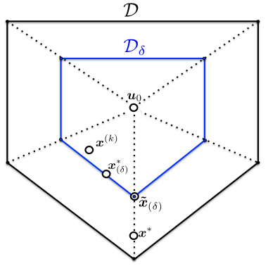
Figure 3: Illustration of the four points considered for the error analysis of the fixed-$\delta$ variant

We note that the modulus of continuity function $\omega$ quantifies the level of continuity of $f$. For a Lipschitz continuous function, we have $\omega(\sigma)\leq L\sigma$. If instead we have $\omega(\sigma)\leq C\sigma^{\alpha}$ for some $\alpha\in[0,1]$, then $f$ is actually $\alpha$-Hölder continuous. We will see in Section E.2 that the TRW objective is not Lipschitz continuous, but it is $\alpha$-Hölder continuous for any $\alpha<1$, and so is “almost” Lipschitz continuous. From the theorem, we see that to get an accuracy of the order $\epsilon$, we would need $(\delta\operatorname{diam}(\mathcal{D}))^{\alpha}<\epsilon$, and thus a contraction of $\delta<\frac{\epsilon^{(1/\alpha)}}{\operatorname{diam}(\mathcal{D})}$.

Appendix D Convergence with Adaptive-$\delta$

In this section, we show the convergence of the adaptive-$\delta$ FW algorithm to optimize a function $f$ satisfying the properties in Problem 3.2 and Property 3.3 (Lipschitz gradient over $\mathcal{D}_{\delta}$ with bounded growth).

The adaptive update for $\delta$ (given in Algorithm 1) can be used with the standard Frank-Wolfe optimization algorithm or also the fully corrective Frank-Wolfe (FCFW) variant. In FCFW, we ensure that every update makes more progress than a standard FW step with line-search, and thus we will show the convergence result in this section for standard FW (which also applies to FCFW). We describe the FCFW variant with approximate correction steps in Algorithm 4, as this is what we used in our experiments.

We first list a few definitions and lemmas that will be used for the main convergence convergence result given in Theorem D.6. We begin with the definitions of duality gaps that we use throughout this section. The Frank-Wolfe gap is our primary criterion for halting and measuring the progress of the optimization over $\mathcal{D}$. The uniform gap is a measure of the decrease obtainable from moving towards the uniform distribution.

Definition D.1.

We define the following gaps:

1. The Frank-Wolfe (FW) gap is defined as: $g(\bm{x}^{(k)}):=\langle-\nabla f(\bm{x}^{(k)}),\bm{s}^{(k)}-\bm{x}^{(k)}\rangle$.

2. The uniform gap is defined as: $g_{u}(\bm{x}^{(k)}):=\langle-\nabla f(\bm{x}^{(k)}),\bm{u}_{0}-\bm{x}^{(k)}\rangle$.

3. The FW gap over $\mathcal{D}_{\delta}$ is: $g_{(\delta^{(k)})}(\bm{x}^{(k)}):=\langle-\nabla f(\bm{x}^{(k)}),\bm{s}^{(k)}_{(\delta)}-\bm{x}^{(k)}\rangle$.

The name for the uniform gap comes from the fact that the FW gap over $\mathcal{D}_{\delta}$ can be expressed as a convex combination of the FW gap over $\mathcal{D}$ and the uniform gap:

$$g_{(\delta^{(k)})}(\bm{x}^{(k)}) =\langle-\nabla f(\bm{x}^{(k)}),\,\,(1-\delta^{(k)})\bm{s}^{(k)}+\delta^{(k)}\bm{u}_{0}-\bm{x}^{(k)}\rangle$$

$$=(1-\delta^{(k)})g(\bm{x}^{(k)})+\delta^{(k)}g_{u}(\bm{x}^{(k)}).$$ (8)

The uniform gap represents the negative directional derivative of $f$ at $\bm{x}^{(k)}$ in the direction $\bm{u}_{0}-\bm{x}^{(k)}$. When the uniform gap is negative (thus $f$ is increasing when moving towards $\bm{u}_{0}$ from $\bm{x}^{(k)}$), then the contraction is hurting progress, which explains the type of adaptive update for $\delta$ given by Algorithm 1 where we consider shrinking $\delta$ in this case. This enables us to crucially relate the FW gap over $\mathcal{D}_{\delta}$ with the one over $\mathcal{D}$, as given in the following lemma, using the assumption that $\delta^{(\mathrm{init})}\leq\frac{1}{4}$.

Lemma D.2 (Gaps relationship).

For iterates progressing as in Algorithm 4 with adaptive update on $\delta$ as given in Algorithm 1, the gap over $\mathcal{D}_{\delta}$ and $\mathcal{D}$ are related as : $g_{(\delta^{(k)})}(\bm{x}^{(k)})\geq\frac{g(\bm{x}^{(k)})}{2}$.

Proof.

The duality gaps $g(\bm{x}^{(k)})$ and $g_{(\delta^{(k)})}(\bm{x}^{(k)})$ computed as defined in (D.1) during Algorithm 4 are related by equation (8).

We analyze two cases separately:

(1) When $g_{u}(\bm{x}^{(k)})\geq 0$, for $\delta^{(\mathrm{init})}\leq\frac{1}{4}$, we have $g_{(\delta^{(k)})}(\bm{x}^{(k)})\geq\frac{3}{4}g(\bm{x}^{(k)})$ as $\delta^{(k)}\leq\delta^{(\mathrm{init})}$.

(2) When $g_{u}(\bm{x}^{(k)})<0$, from the update rule in lines 5 to 7 in Algorithm 1, we have $\delta^{(k)}\leq\frac{g(\bm{x}^{(k)})}{-4g_{u}(\bm{x}^{(k)})}\implies\delta^{(k)}g_{u}(\bm{x}^{(k)})\geq-\frac{g(\bm{x}^{(k)})}{4}$. Therefore, $g_{(\delta^{(k)})}(\bm{x}^{(k)})\geq\frac{3}{4}g(\bm{x}^{(k)})-\frac{g(\bm{x}^{(k)})}{4}=\frac{g(\bm{x}^{(k)})}{2}$.

Therefore, the gap over $\mathcal{D}_{\delta}$ and $\mathcal{D}$ are related as : $g_{(\delta^{(k)})}(\bm{x}^{(k)})\geq\frac{g(\bm{x}^{(k)})}{2}$. ∎

Another property that we will use in the convergence proof is that $-g_{u}$ is upper bounded for any convex function $f$:

Lemma D.3 (Bounded negative uniform gap).

Let $f$ be a continuously differentiable convex function on the relative interior of $\mathcal{D}$. Then for any fixed $\bm{u}_{0}$ in the relative interior of $\mathcal{D}$, $\exists B$ s.t.

$$\forall\bm{x}\in\mathcal{D},\;\;-g_{u}(\bm{x})=\left\langle\nabla f(\bm{x}),\bm{u}_{0}-\bm{x}\right\rangle\leq B.$$ (9)

In particular, we can take the finite value:

$$B:=\|\nabla f(\bm{u}_{0})\|_{*}\operatorname{diam}_{\|\cdot\|}(\mathcal{D})$$ (10)

Proof.

As $f$ is convex, its directional derivative is a monotone increasing function in any direction. Let $\bm{u}_{0}$ and $\bm{x}$ be points in the relative interior of $\mathcal{D}$; then their gradient exists and we have by the monotonicity property:

$$\left\langle\nabla f(\bm{u}_{0})-\nabla f(\bm{x}),\bm{u}_{0}-\bm{x}\right\rangle\geq 0$$

$$\implies\left\langle\nabla f(\bm{u}_{0}),\bm{u}_{0}-\bm{x}\right\rangle\geq\left\langle\nabla f(\bm{x}),\bm{u}_{0}-\bm{x}\right\rangle.$$

This inequality is valid for all $\bm{x}$ in the relative interior of $\mathcal{D}$, and can be extended to the boundary by taking limits (with potentially the RHS become minus infinity, but this is not a problem). Finally, by the definition of the dual norm (generalized Cauchy-Schwartz), we have $\left\langle\nabla f(\bm{u}_{0}),\bm{u}_{0}-\bm{x}\right\rangle\leq\|\nabla f(\bm{u}_{0})\|_{*}\|\bm{u}_{0}-\bm{x}\|\leq\|\nabla f(\bm{u}_{0})\|_{*}\operatorname{diam}_{\|\cdot\|}(\mathcal{D})$. ∎

Finally, we need a last property of Algorithm 4 that allows us to bound the amount of perturbation $\delta^{(k)}$ of the polytope at every iteration as a function of the sub-optimality over $\mathcal{D}$.

Lemma D.4 (Lower bound on perturbation).

Let $B$ be a bound such that $-8g_{u}(\bm{x})\leq B$ for all $\bm{x}\in\mathcal{D}$ (given by Lemma D.3). Then at every stage of Algorithm 4, we have that:

$$\delta^{(\mathrm{init})}\geq\delta^{(k)}\geq\min\left\{\frac{h_{k}}{B},\delta^{(\mathrm{init})}\right\},$$

where $\delta^{(\mathrm{init})}$ is the initial value of $\delta$ and $h_{k}:=f(\bm{x}^{(k)})-f(\bm{x}^{*})$ is the sub-optimality of the iterate.

Proof.

When defining $\delta^{(k)}$ in step 10 of Algorithm 4, we either preserve the value of $\delta^{(k-1)}$ or if we update it, then by the lines 6 and 7 of Algorithm 1, we have $\delta^{(k)}\geq\frac{\tilde{\delta}}{2}=\frac{1}{2}\frac{g(\bm{x}^{(k)})}{-4g_{u}(\bm{x}^{(k)})}\geq\frac{g(\bm{x}^{(k)})}{B}$ (by using $g_{u}(\bm{x}^{(k)})<0$ in this case). Since $g(\bm{x}^{(k)})\geq h_{k}$ (the FW gap always upper bounds the suboptimality), we conclude $\delta^{(k)}\geq\min\{\frac{h_{k}}{B},\delta^{(k-1)}\}$. Unrolling this recurrence, we thus get:

$$\delta^{(k)}\geq\min\left\{\min_{0\leq l\leq k}\frac{h_{l}}{B},\,\,\delta^{(\mathrm{init})}\right\}=\min\left\{\frac{h_{k}}{B},\delta^{(\mathrm{init})}\right\}.$$

For the last equality, we used the fact that $h_{k}$ is non-increasing since Algorithm 4 decreases the objective at every iteration (using the line-search in step 14). ∎

We now bound the generalization of a standard recurrence that will arise in the proof of convergence. This is a generalization of the technique used in teo2007erm (also used in the context of Frank-Wolfe in the proof of Theorem C.4 in Lacoste-Julien et al. (2013)). The basic idea is that one can bound a recurrence inequality by the solution to a differential equation. We provide a detailed proof of the bound for completeness here.

Lemma D.5 (Recurrence inequality solution).

Let $1<a\leq b$. Suppose that $h_{k}$ is any non-negative sequence that satisfies the recurrence inequality:

$$h_{k+1}\leq h_{k}-\frac{1}{bC_{0}}(h_{k})^{a}\qquad\text{with initial condition}\quad h_{0}^{a-1}\leq C_{0}.$$

Then $h_{k}$ is strictly decreasing (unless it equals zero) and can be bounded for $k\geq 0$ as:

$$h_{k}\leq\left(\frac{C_{0}}{(\frac{a-1}{b})k+1}\right)^{\frac{1}{a-1}}$$

Proof.

Taking the continuous time analog of the recurrence inequality, we consider the differential equation:

$$\frac{\mathrm{\bm{d}}h}{\mathrm{\bm{d}}t}=\frac{-h^{a}}{bC_{0}}\qquad\text{with initial condition}\quad h(0)=C_{0}^{\frac{1}{a-1}}.$$

Solving it:

$$\begin{split}&\frac{\mathrm{\bm{d}}h}{\mathrm{\bm{d}}t}=\frac{-h^{a}}{bC_{0}}\\ \implies&\int\frac{\mathrm{\bm{d}}h}{h^{a}}=\int\frac{-\mathrm{\bm{d}}t}{bC_{0}}\\ \implies&\left[\frac{-h^{1-a}}{a-1}\right]^{h(t)}_{h(0)}=-\frac{t-0}{bC_{0}}\\ &\quad\emph{{( Using the initial conditions:)}}\\ \implies&\frac{-1}{h(t)^{a-1}}+\frac{1}{C_{0}}=\frac{-t(a-1)}{bC_{0}}\\ \implies&\frac{1}{h(t)^{a-1}}=\left((\frac{a-1}{b})t+1\right)\frac{1}{C_{0}}\\ \implies&h(t)=\left(\frac{C_{0}}{(\frac{a-1}{b})t+1}\right)^{\frac{1}{a-1}}.\end{split}$$

We now denote the solution to the differential equation as $\tilde{h}(t)$. Note that it is a strictly decreasing convex function (which could also be directly implied from the differential equation as: $\frac{\mathrm{\bm{d}}^{2}h}{\mathrm{\bm{d}}t^{2}}=-a\underbrace{\frac{h^{a-1}}{bC_{0}}}_{>0}\underbrace{h^{\prime}(t)}_{<0}>0$ ). Our strategy will be to show by induction that if $h_{k}\leq\tilde{h}(k)$, then $h_{k+1}\leq\tilde{h}(k+1)$. This allows us to bound the recurrence by the solution to the differential equation.

Assume that $h_{k}\leq\tilde{h}(k)$. The base case is $h_{0}\leq\tilde{h}(0)=C_{0}^{\frac{1}{a-1}}$, which is true by the initial condition on $h_{0}$.

Consider the utility function $l(h):=h-\frac{h^{a}}{bC_{0}}$ which is maximized at $\bar{h}:=\left(\frac{bC_{0}}{a}\right)^{\frac{1}{a-1}}$. This function can be verified to be strictly concave for $a>1$ and therefore is increasing for $h\leq\bar{h}$. Note that the recurrence inequality can be written as $h_{k+1}\leq l(h_{k})$. Since $\tilde{h}$ is decreasing and that $\tilde{h}(0))=C_{0}^{\frac{1}{a-1}}\leq\left(\frac{bC_{0}}{a}\right)^{\frac{1}{a-1}}=\bar{h}$ (the last inequality holds since $b\geq a$), we have $\tilde{h}(t)\leq\bar{h}$ for all $t\geq 0$, and so $\tilde{h}(t)$ is always in the monotone increasing region of $l$.

From the induction hypothesis and the monotonicity of $l$, we thus get that $l(h_{k})\leq l(\tilde{h}(k))$.

Now the convexity of $\tilde{h}(t)$ gives us $\tilde{h}(k+1)\geq\tilde{h}(k)+\tilde{h}^{\prime}(k)=\tilde{h}(k)-\frac{\tilde{h}(k)^{a}}{bC_{0}}=l(\tilde{h}(k))$. Combining these two facts with the recurrence inequality $h_{k+1}\leq l(h_{k})$, we get: $h_{k+1}\leq l(h_{k})\leq l(\tilde{h}(k))\leq\tilde{h}(k+1)$, completing the induction step and the main part of the proof.

Finally, whenever $h_{k}>0$, we have that $h_{k+1}<h_{k}$ from the recurrence inequality, and so $h_{k}$ is strictly decreasing as claimed. ∎

Given these elements, we are now ready to state the main convergence result for Algorithm 4. The convergence rate goes through three stages with increasingly slower rate. The level of suboptimality $h_{k}$ determines the stage. We first give the high level intuition behind these stages. Recall that by Lemma D.4, $h_{k}$ lower bounds the amount of perturbation $\delta^{(k)}$, and thus when $h_{k}$ is big, the function $f$ is well-behaved by Property 3.3. In the first stage, the suboptimality is bigger than some target constant (which implies that the FW gap is big), yielding a geometric rate of decrease of error (as is standard for FW with line-search in the first few steps). In the second stage, the suboptimality is in an intermediate regime: it is smaller than the target constant, but big enough compared to the initial $\delta^{\mathrm{init}}$ so that $f$ is still well-behaved on $\mathcal{D}_{\delta^{(k)}}$. We get there the usual $O(1/k)$ rate as in standard FW. Finally, in the third stage, we get the slower $O(k^{-\frac{1}{p+1}})$ rate where the growth in $O(\delta^{-p})$ of the Lipschitz constant of $f$ over $\mathcal{D}_{\delta}$ comes into play.

Theorem D.6 (Global convergence for adaptive-$\delta$ variant over $\mathcal{D}$).

Consider the optimization of $f$ satisfying the properties in Problem 3.2 and Property 3.3. Let $\widetilde{C}:=L\operatorname{diam}_{\|\cdot\|}(\mathcal{D})^{2}$, where $L$ is from Property 3.3. Let $B$ be the upper bound on the negative uniform gap: $-8g_{u}(\bm{x})\leq B$ for all $\bm{x}\in\mathcal{D}$, as used in Lemma D.4 (arising from Lemma D.3). Then the iterates $\bm{x}^{(k)}$ obtained by running the Frank-Wolfe updates over $\mathcal{D}_{\delta}$ with line-search with $\delta$ updated according to Algorithm 1 (or as summarized in a FCFW variant in Algorithm 4), have suboptimality $h_{k}$ upper bounded as:

1. $h_{k}\leq\left(\frac{1}{2}\right)^{k}h_{0}+\frac{\widetilde{C}}{\delta_{0}^{p}}$ for $k$ such that $h_{k}\geq\max\{B\delta_{0},\frac{2\widetilde{C}}{\delta_{0}^{p}}\}$,
   

2. $h_{k}\leq\frac{2\widetilde{C}}{\delta_{0}^{p}}\left[\frac{1}{\frac{1}{4}(k-k_{0})+1}\right]$ for $k$ such that $B\delta_{0}\leq h_{k}\leq\frac{2\widetilde{C}}{\delta_{0}^{p}}$,
   

3. $h_{k}\leq\left[\frac{\max(\widetilde{C},B\delta_{0}^{p+1})B^{p}}{\frac{p+1}{\max(8,p+2)}(k-k_{1})+1}\right]^{\frac{1}{p+1}}=O(k^{-\frac{1}{p+1}})$ for $k$ such that $h_{k}\leq B\delta_{0}$,
   

where $\delta_{0}=\delta^{(\mathrm{init})}$, $h_{0}$ is the initial suboptimality, and $k_{0}$ and $k_{1}$ are the number of steps to reach stage 2 and 3 respectively which are bounded as: $k_{0}\leq\max(0,\lceil\log_{\frac{1}{2}}\frac{\widetilde{C}}{h_{0}\delta_{0}^{p}}\rceil)$, $k_{0}\leq k_{1}\leq k_{0}+\max\left(0,\lceil\frac{8\widetilde{C}}{B\delta_{0}^{p+1}}\rceil-4\right)$.

Proof.

Let $\bm{x}_{\gamma}:=\bm{x}^{(k)}+\gamma\bm{d}_{k}^{\hskip 0.35002pt\textnormal{FW}}$ with $\bm{d}_{k}^{\hskip 0.35002pt\textnormal{FW}}$ defined in step 12 in Algorithm 4. Note that $\bm{x}_{\gamma}\in\mathcal{D}_{\delta}$ with $\delta=\delta^{(k)}$ for all $\gamma\in[0,1]$. We apply the Descent Lemma A.1 on this update to get:

$$f(\bm{x}_{\gamma})\leq f(\bm{x}^{(k)})+\gamma\langle\nabla f(\bm{x}^{(k)}),\bm{d}_{k}^{\hskip 0.35002pt\textnormal{FW}}\rangle+\gamma^{2}\frac{L\|\bm{d}_{k}^{\hskip 0.35002pt\textnormal{FW}}\|^{2}}{2\left(\delta^{(k)}\right)^{p}}\qquad\forall\gamma\in[0,1].$$

We have $L\|\bm{d}_{k}^{\hskip 0.35002pt\textnormal{FW}}\|^{2}\leq\widetilde{C}$ by assumption and $\langle\nabla f(\bm{x}^{(k)}),\bm{d}_{k}^{\hskip 0.35002pt\textnormal{FW}}\rangle=-g_{(\delta)}(\bm{x}^{(k)})$ by definition. Moreover, $\bm{x}^{(k+1)}$ is defined to make at least as much progress than the line-search result $\min_{\gamma\in[0,1]}f(\bm{x}_{\gamma})$ (line 14 and 15), and so we have:

$$f(\bm{x}^{(k+1)}) \leq f(\bm{x}^{(k)})-\gamma g_{(\delta)}(\bm{x}^{(k)})+\gamma^{2}\frac{\widetilde{C}}{2\left(\delta^{(k)}\right)^{p}}\quad\forall\gamma\in[0,1]$$

$$\leq f(\bm{x}^{(k)})-\frac{\gamma}{2}g(\bm{x}^{(k)})+\gamma^{2}\frac{\widetilde{C}}{2\left(\delta^{(k)}\right)^{p}}\quad\forall\gamma\in[0,1].$$

For the final inequality, we used Lemma D.2 which relates the gap over $\mathcal{D}_{\delta}$ to the gap over $\mathcal{D}$.

Subtracting $f(\bm{x}^{*})$ from both sides and using $g(\bm{x}^{(k)})\geq h_{k}$ by convexity, we get:

$$h_{k+1}\leq h_{k}-\frac{\gamma h_{k}}{2}+\frac{\gamma^{2}\widetilde{C}}{2\left(\delta^{(k)}\right)^{p}}.$$

Now, using Lemma D.4, we have that $\delta^{(k)}\geq\min(\frac{h_{k}}{B},\delta^{(\mathrm{init})})$:

$$h_{k+1} \leq h_{k}-\gamma\frac{h_{k}}{2}+\frac{\gamma^{2}}{2}\frac{\widetilde{C}}{\left(\min(\frac{h_{k}}{B},\delta^{(\mathrm{init})})\right)^{p}}\quad\forall\gamma\in[0,1].$$ (11)

We refer to (11) as the master inequality. Since we no longer have a dependance on $\delta^{(k)}$, we refer to $\delta^{(\mathrm{init})}$ as $\delta_{0}$. We now follow a similar form of analysis as in the proof of Theorem C.4 in Lacoste-Julien et al. (2013). To solve this and bound the suboptimality, we consider three stages:

1. Stage 1: The $\min$ in the denominator is $\delta_{0}$ and $h_{k}$ is big: $h_{k}\geq\max\{B\delta_{0},\frac{2\widetilde{C}}{\delta_{0}^{p}}\}$.

2. Stage 2: The $\min$ in the denominator is $\delta_{0}$ and $h_{k}$ is small: $B\delta_{0}\leq h_{k}\leq\frac{2\widetilde{C}}{\delta_{0}^{p}}$.

3. Stage 3: The $\min$ in the denominator is $\frac{h_{k}}{B}$, i.e.: $h_{k}\leq B\delta_{0}$.

Since $h_{k}$ is decreasing, once we leave a stage, we no longer re-enter it. The overall strategy for each stage is as follows. For each recurrence that we get, we select a $\gamma^{*}$ that realizes the tightest upper bound on it.

Since we are restricted that $\gamma^{*}\in[0,1]$, we have to consider when $\gamma^{*}>1$ and $\gamma^{*}\leq 1$. For the former, we bound the recurrence obtained by substituting $\gamma=1$ into (11). For the latter, we substitute the form of $\gamma^{*}$ into the recurrence and bound the result.

Stage 1

We consider the case where $h_{k}\geq B\delta_{0}$. This yields:

$$h_{k+1} \leq h_{k}-\frac{\gamma h_{k}}{2}+\frac{\gamma^{2}\widetilde{C}}{2\left(\delta_{0}\right)^{p}}$$ (12)

The bound is minimized by setting $\gamma^{*}=\frac{h_{k}\delta_{0}^{p}}{2\widetilde{C}}$. On the other hand, the bound is only valid for $\gamma\in[0,1]$, and thus if $\gamma^{*}>1$, i.e. $h_{k}>\frac{2\widetilde{C}}{\delta_{0}^{p}}$ (stage 1), then $\gamma=1$ will yield the minimum feasible value for the bound. Unrolling the recursion (12) for $\gamma=1$ during this stage (where $h_{l}>\frac{2\widetilde{C}}{\delta_{0}^{p}}$ for $l<k$ as $h_{k}$ is decreasing), we get:

$$h_{k+1} \leq\frac{h_{k}}{2}+\frac{\widetilde{C}}{2\delta_{0}^{p}}$$

$$\leq\frac{1}{2}\left(\frac{h_{k-1}}{2}+\frac{\widetilde{C}}{2\delta_{0}^{p}}\right)+\frac{\widetilde{C}}{2\delta_{0}^{p}}$$

$$\leq\left(\frac{1}{2}\right)^{k+1}h_{0}+\frac{\widetilde{C}}{2\delta_{0}^{p}}\underbrace{\sum_{l=0}^{k}\left(\frac{1}{2}\right)^{l}}_{\leq\sum_{l=0}^{\infty}\left(\frac{1}{2}\right)^{l}=2}$$

$$\text{thus}\quad h_{k} \leq\left(\frac{1}{2}\right)^{k}h_{0}+\frac{\widetilde{C}}{\delta_{0}^{p}},$$ (13)

giving the bound for the iterates in the first stage.

We can compute an upper bound on the number of steps it takes to reach a suboptimality of $\frac{2\widetilde{C}}{\delta_{0}^{p}}$ by looking at the minimum $k$ which ensures that the bound in (13) becomes smaller than $\frac{2\widetilde{C}}{\delta_{0}^{p}}$, yielding $k_{\max}=\max(0,\lceil\log_{\frac{1}{2}}\frac{\widetilde{C}}{h_{0}\delta_{0}^{p}}\rceil)$. Therefore, let $k_{0}\leq k_{\max}$ be the first $k$ such that $h_{k}\leq\frac{2\widetilde{C}}{\delta_{0}^{p}}$.

Stage 2

For this case analysis, we refer to $k$ as being the iterations after $k_{0}$ steps have elapsed. I.e. if $k_{\mathrm{new}}:=k-k_{0}$, then we refer to $k_{\mathrm{new}}$ as $k$ moving forward.

In stage 2, we suppose that $B\delta_{0}\leq h_{k}\leq\frac{2\widetilde{C}}{\delta_{0}^{p}}$. This means that $\gamma^{*}=\frac{h_{k}\delta_{0}^{p}}{2\widetilde{C}}\leq 1$.

Substituting $\gamma=\gamma^{*}$ into (12) yields: $h_{k+1}\leq h_{k}-h_{k}^{2}\frac{\delta_{0}^{p}}{8\widetilde{C}}$.

Using the result of Lemma D.5 with $a=2$, $b=4$ and $C_{0}=\frac{2\widetilde{C}}{\delta_{0}^{p}}$, we get the bound:

$$h_{k}\leq\frac{\frac{2\widetilde{C}}{\delta_{0}^{p}}}{\frac{k-k_{0}}{4}+1}.$$

It is worthwhile to point out at this juncture that the bound obtained for stage $2$ is the same as the one for regular Frank-Wolfe, but with a factor of $4$ worse due to the factor of $\frac{1}{2}$ in front of the FW gap which appeared due to Lemma D.2.

Stage 3

Here, we suppose $h_{k}\leq B\delta_{0}$. We can compute a bound on the number of steps $k_{1}$ needed get to stage 3 by looking at the number of steps it takes for the bound in stage 2 to becomes less than $B\delta_{0}$:

$$\begin{split}\frac{2\widetilde{C}}{\delta_{0}^{p}}\left[\frac{4}{k_{1}-k_{0}+4}\right]\leq B\delta_{0}\\ \left[\frac{1}{k_{1}-k_{0}+4}\right]\leq\frac{B\delta_{0}^{p+1}}{8\widetilde{C}}\\ k_{1}\geq k_{0}+\lceil\frac{8\widetilde{C}}{B\delta_{0}^{p+1}}\rceil-4.\end{split}$$

As before, moving forward, our notation on $k$ represents the number of steps taken after $k_{1}$ steps.

Then, the master inequality (11) becomes:

$$h_{k+1}\leq h_{k}-\frac{\gamma}{2}h_{k}+\frac{\gamma^{2}\widetilde{C}B^{p}}{2h_{k}^{p}}.$$

To simplify the rest of the analysis, we replace $\widetilde{C}B^{p}$ with $F:=\max(B\delta_{0}^{p+1},\widetilde{C})B^{p}$. We then get the bound:

$$h_{k+1}\leq h_{k}-\frac{\gamma}{2}h_{k}+\frac{\gamma^{2}F}{2h_{k}},$$ (14)

which is minimized by setting $\gamma^{*}:=\frac{h_{k}^{p+1}}{2F}$. Since $F\geq B^{p+1}\delta_{0}^{p+1}$ (by construction) and $h_{k}^{p+1}\leq(B\delta_{0})^{p+1}$ (by the condition to be in stage 3), we necessarily have that $\gamma^{*}\leq 1$. We chose the value of $F$ to avoid having to consider the possibility $\gamma^{*}>1$ as we did in the distinction between stage 1 and stage 2.

Hence, substituting $\gamma=\gamma^{*}$ in (14), we get:

$$h_{k+1}\leq h_{k}-\frac{h_{k}^{p+2}}{8F}.$$

Using the result of Lemma D.5 with $a=p+2$, $b=\max(8,p+2)$ and $C_{0}=F$, we get the bound:

$$h_{k}\leq\left[\frac{\max(\widetilde{C},B\delta_{0}^{p+1})B^{p}}{\frac{p+1}{\max(8,p+2)}(k-k_{1})+1}\right]^{\frac{1}{p+1}}=O(k^{-\frac{1}{p+1}}),$$

concluding the proof. ∎

Interestingly, the obtained rate of $O(1/\sqrt{k})$ for $p=1$ (for the TRW objective e.g.) is the standard rate that one would get for the optimization of a general non-smooth convex function with the projected subgradient method (and it is even a lower bound for some class of first-order methods; see e.g. Section 3.2 in nesterov2004lectures). The fact that our function $f$ does not have Lipschitz continuous gradient on the whole domain brings us back to the realm of non-smooth optimization. It is an open question whether Algorithm 4 has an optimal rate for the class of functions defined in the assumptions of Theorem D.6.

Appendix E Properties of the TRW Objective

In this section, we explicitly compute bounds for the constants appearing in the convergence statements for our fixed-$\delta$ and adaptive-$\delta$ algorithms for the optimization problem given by:

$$\min_{\vec{\bm{\mu}}\in\mathcal{M}}-\text{TRW}(\vec{\bm{\mu}};\vec{\bm{\theta}},\bm{\rho}).$$

In particular, we compute the Lipschitz constant for its gradient over $\mathcal{M}_{\delta}$ (Property 3.3), we give a form for its modulus of continuity function $\omega(\cdot)$ (used in Theorem 3.4), and we compute $B$, the upper bound on the negative uniform gap (as used in Lemma D.3).

E.1 Property 3.3 : Controlled Growth of Lipschitz Constant over $\mathcal{M}_{\delta}$

We first motivate our choice of norm over $\mathcal{M}$. Recall that $\vec{\bm{\mu}}$ can be decomposed into $|V|+|E|$ blocks, with one pseudo-marginal vector $\bm{\mu}_{i}\in\Delta_{\textrm{VAL}_{i}}$ for each node $i\in V$, and one vector $\bm{\mu}_{ij}\in\Delta_{\textrm{VAL}_{i}\textrm{VAL}_{j}}$ per edge $\{i,j\}\in E$, where $\Delta_{d}$ is the probability simplex over $d$ values. We let $c$ be the cliques in the graph (either nodes or edges). From its definition in (2), $f(\vec{\bm{\mu}}):=-\text{TRW}(\vec{\bm{\mu}};\vec{\bm{\theta}},\bm{\rho})$ decomposes as a separable sum of functions of each block only:

$$f(\vec{\bm{\mu}}):=-\text{TRW}(\vec{\bm{\mu}};\vec{\bm{\theta}},\bm{\rho})=-\sum_{c}\left(K_{c}H(\bm{\mu}_{c})+\left\langle\bm{\theta}_{c},\bm{\mu}_{c}\right\rangle\right)=:\sum_{c}g_{c}(\bm{\mu}_{c}),$$ (15)

where $K_{c}$ is $(1-\sum_{j\in\mathcal{N}(i)}\rho_{ij})$ if $c=i$ and $\rho_{ij}$ if $c=\{i,j\}$. The function $g_{c}$ also decomposes as a separable sum:

$$g_{c}(\bm{\mu}_{c}):=\sum_{x_{c}}K_{c}\mu_{c}(x_{c})\log(\mu_{c}(x_{c}))-\theta_{c}(x_{c})\mu_{c}(x_{c})=:\sum_{x_{c}}g_{c,x_{c}}(\mu_{c}(x_{c})).$$ (16)

As $\mathcal{M}$ is included in a product of probability simplices, we will use the natural $\ell_{\infty}/\ell_{1}$ block-norm, i.e. $\|\vec{\bm{\mu}}\|_{\infty,1}:=\max_{c}\|\bm{\mu}_{c}\|_{1}$. The diameter of $\mathcal{M}$ in this norm is particularly small: $\operatorname{diam}_{\|\cdot\|_{\infty,1}}(\mathcal{M})\leq 2$. The dual norm of the $\ell_{\infty}/\ell_{1}$ block-norm is the $\ell_{1}/\ell_{\infty}$ block-norm, which is what we will need to measure the Lipschitz constant of the gradient (because of the dual norm pairing requirement from the Descent Lemma A.1).

Lemma E.1.

Consider the $\ell_{\infty}/\ell_{1}$ norm on $\mathcal{M}$ and its dual norm $\ell_{1}/\ell_{\infty}$ to measure the gradient. Then $\nabla\text{TRW}(\vec{\bm{\mu}};\vec{\bm{\theta}},\bm{\rho})$ is Lipschitz continuous over $\mathcal{M}_{\delta}$ with respect to these norms with Lipschitz constant $L_{\delta}\leq\frac{L}{\delta}$ with:

$$L\leq 4|V|\,\max_{ij\in E}\,\,(\textrm{VAL}_{i}\textrm{VAL}_{j}).$$ (17)

Proof.

We first consider one scalar component of the separable $g_{c}(\bm{\mu}_{c})$ function given in (16) (i.e. for one $\mu_{c}(x_{c})$ coordinate). Its derivative is $K_{c}(1+\log(\mu_{c}(x_{c}))-\theta_{c}(x_{c})$ with second derivative $\frac{K_{c}}{\mu_{c}(x_{c})}$. If $\vec{\bm{\mu}}\in\mathcal{M}_{\delta}$, then we have $\mu_{c}(x_{c})\geq\delta u_{0}(x_{c})=\frac{\delta}{n_{c}}$, where $n_{c}$ is the number of possible values that the assignment variable $x_{c}$ can take. Thus for $\vec{\bm{\mu}}\in\mathcal{M}_{\delta}$, we have that the $x_{c}$-component of $g_{c}$ is Lipschitz continuous with constant $|K_{c}|n_{c}/\delta$. We thus have:

$$\|\nabla g_{c}(\bm{\mu}_{c})-\nabla g_{c}(\bm{\mu}^{\prime}_{c})\|_{\infty} =\max_{x_{c}}\,\,|g^{\prime}_{c,x_{c}}(\mu(x_{c}))-g^{\prime}_{c,x_{c}}(\mu^{\prime}(x_{c}))|$$

$$\leq\frac{|K_{c}|n_{c}}{\delta}\|\bm{\mu}_{c}-\bm{\mu}_{c}^{\prime}\|_{\infty}\leq\frac{|K_{c}|n_{c}}{\delta}\|\bm{\mu}_{c}-\bm{\mu}_{c}^{\prime}\|_{1}.$$

Considering now the $\ell_{1}$-sum over blocks, we have:

$$\|\nabla f(\vec{\bm{\mu}})-\nabla f(\vec{\bm{\mu}}^{\prime})\|_{1,\infty} =\sum_{c}\|\nabla g_{c}(\bm{\mu}_{c})-\nabla g_{c}(\bm{\mu}^{\prime}_{c})\|_{\infty}$$

$$\leq\sum_{c}\frac{K_{c}n_{c}}{\delta}\|\bm{\mu}_{c}-\bm{\mu}_{c}^{\prime}\|_{1}\leq\frac{1}{\delta}\left(\sum_{c}K_{c}n_{c}\right)\|\vec{\bm{\mu}}-\vec{\bm{\mu}}^{\prime}\|_{\infty,1}.$$

The Lipschitz constant is thus indeed $\frac{L}{\delta}$ with $L:=\sum_{c}|K_{c}|n_{c}$. Let us first consider the sum for $c\in V$; we have $K_{i}=1-\sum_{j\in\mathcal{N}(i)}\rho_{ij}$. Thus:

$$\sum_{i}|K_{i}| \leq|V|+\sum_{i}\sum_{j\in\mathcal{N}(i)}\rho_{ij}$$

$$=|V|+2\sum_{ij\in E}\rho_{ij}=|V|+2(|V|-1)\leq 3|V|.$$

Here we used the fact that $\rho_{ij}$ came from the marginal probability of edges of spanning trees (and so with $|V|-1$ edges). Similarly, we have $\sum_{ij\in E}|K_{ij}|\leq|V|$. Combining these we get:

$$L=\sum_{c}|K_{c}|n_{c}\leq(\max_{c}n_{c})\sum_{c}|K_{c}|\leq\max_{ij\in E}\textrm{VAL}_{i}\textrm{VAL}_{j}4|V|.$$ (18)

∎

Remark 1.

The important quantity in the convergence of Frank-Wolfe type algorithms is $\tilde{C}=L\operatorname{diam}(\mathcal{M})^{2}$. We are free to take any dual norm pairs to compute this quantity, but some norms are better aligned with the problem than others. Our choice of norm in Lemma E.1 gives $\tilde{C}\leq 16|V|k^{2}$ where $k$ is the maximum number of possible values a random variable can take. It is interesting that $|E|$ does not appear in the constant. If instead we had used the $\ell_{2}/\ell_{1}$ block-norm on $\mathcal{M}$, we get that $\operatorname{diam}_{\ell_{2}/\ell_{1}}(\mathcal{M})^{2}=4(|V|+|E|)$, while the constant $L$ with dual norm $\ell_{2}/\ell_{\infty}$ would be instead $\max_{c}|K_{c}|n_{c}$ which is bigger than $\max_{c}n_{c}=k^{2}$, thus giving a worse bound.

E.2 Modulus of Continuity Function

We begin by computing a modulus of continuity function for $-x\log x$ with an additive linear term.

Lemma E.2.

Let $g(x):=-Kx\log x+\theta x$. Consider $x,x^{\prime}\in[0,1]$ such that $|x-x^{\prime}|\leq\sigma$, then:

$$|g(x^{\prime})-g(x)|\leq\sigma|\theta|+2\sigma|K|\max\{-\log(2\sigma),1\}=:\omega_{g}(\sigma).$$ (19)

Proof.

Without loss of generality assume $x^{\prime}>x$, then we have two cases:

Case i. If $x>\sigma$, then we have that the Lipschitz constant of $g(x)$ is $L_{\sigma}=|\theta|+|K||(1+\log\sigma)|$ (obtained by taking the supremum of its derivative). Therefore, we have that $|g(x^{\prime})-g(x)|\leq L_{\sigma}\sigma$. Note that $L_{\sigma}\sigma\to 0$ when $\sigma\to 0$ even if $L_{\sigma}\to\infty$, since $L_{\sigma}$ grows logarithmically.

Case ii. If $x\leq\sigma$, then $x^{\prime}\leq x+\sigma\leq 2\sigma$. Therefore:

$$|g(x^{\prime})-g(x)|\leq|K||x\log x-x^{\prime}\log x^{\prime}|+|\theta||x^{\prime}-x|.$$ (20)

Now, we have that $-x\log x$ is non-negative for $x\in[0,1]$. Furthermore, we have that $-x\log x$ is increasing when $x<\exp(-1)$ and decreasing afterwards. First suppose that $2\sigma\leq\exp(-1)$; then $-x^{\prime}\log x^{\prime}\geq-x\log x\geq 0$ which implies:

$$|x\log x-x^{\prime}\log x^{\prime}|\leq-x^{\prime}\log x^{\prime}\leq-2\sigma\log(2\sigma).$$

In the case $2\sigma>\exp(-1)$, then we have:

$$|x\log x-x^{\prime}\log x^{\prime}|\leq\max_{y\in[0,1]}\{-y\log y\}=\exp(-1)\leq 2\sigma.$$

Combining these two possibilities, we get:

$$|x\log x-x^{\prime}\log x^{\prime}|\leq 2\sigma\max\{-\log(2\sigma),1\}.$$

The inequality (20) thus becomes:

$$|g(x^{\prime})-g(x)|\leq|K|2\sigma\max\{-\log(2\sigma),1\}+|\theta|\sigma,$$

which is what we wanted to prove. ∎

For small $\sigma$, the dominant term of the function $\omega_{g}(\sigma)$ in Lemma E.2 is of the form $C\cdot-\sigma\log\sigma$ for a constant $C$. If we require that this be smaller than some small $\xi>0$, then we can choose an approximate $\sigma$ by solving for $x$ in $-Ax\log x=\xi$ yielding $x=\exp(W_{-1}\frac{\xi}{A})$ where $W_{-1}$ is the negative branch of the Lambert W-function. This is almost linear and yields approximately $x=O(\xi)$ for small $\xi$. In fact, we have that $\omega_{g}(\sigma)\leq C^{\prime}\sigma^{\alpha}$ for any $\alpha<1$, and thus $g$ is “almost” Lipschitz continuous.

Lemma E.3.

The following function is a modulus of continuity function for the $\text{TRW}(\vec{\bm{\mu}};\vec{\bm{\theta}},\bm{\rho})$ objective over $\mathcal{M}$ with respect to the $\ell_{\infty}$ norm:

$$\omega(\sigma):=\sigma\|\theta\|_{1}+2\sigma\tilde{K}\max\{-\log(2\sigma),1\},$$ (21)

where $\tilde{K}:=4|V|\max_{ij\in E}\textrm{VAL}_{i}\textrm{VAL}_{j}$.

That is, for $\vec{\bm{\mu}},\vec{\bm{\mu}}^{\prime}\in\mathcal{M}$ with $\|\vec{\bm{\mu}}^{\prime}-\vec{\bm{\mu}}\|_{\infty}\leq\sigma$, we have:

$$|\text{TRW}(\vec{\bm{\mu}};\vec{\bm{\theta}},\bm{\rho})-\text{TRW}(\vec{\bm{\mu}}^{\prime};\vec{\bm{\theta}},\bm{\rho})|\leq\omega(\sigma).$$

Proof.

$\text{TRW}(\vec{\bm{\mu}};\vec{\bm{\theta}},\bm{\rho})$ can be decomposed into functions of the form $-Kx\log x+\theta x$ (see (15) and (16)) and so we apply the Lemma E.2 element-wise. Let $c$ index the clique component in the marginal vector.

$$|\text{TRW}(\vec{\bm{\mu}};\vec{\bm{\theta}},\bm{\rho})-\text{TRW}(\vec{\bm{\mu}}^{\prime};\vec{\bm{\theta}},\bm{\rho})| =\sum_{c}\sum_{x_{c}}|g_{c,x_{c}}(\mu_{c}(x_{c}))-g_{c,x_{c}}(\mu^{\prime}_{c}(x_{c}))|$$

(Using Lemma E.2 and $$\|\vec{\bm{\mu}}^{\prime}-\vec{\bm{\mu}}\|_{\infty}\leq\sigma$$)

$$\leq\sum_{c}\sum_{x_{c}}(|K_{c}|2\sigma\max\{-\log(2\sigma),1\}+|\theta(x_{c})|\sigma)$$

$$=2\sigma\max\{-\log(2\sigma),1\}\sum_{c}|K_{c}|n_{c}+\|\theta\|_{1}\sigma,$$

where we recall $n_{c}$ is the number of values that $x_{c}$ can take. By re-using the bound on $\sum_{c}|K_{c}|n_{c}$ from (18), we get the result. ∎

E.3 Bounded Negative Uniform Gap

Lemma E.4 (Bound for the negative uniform gap of TRW objective).

For the negative TRW objective $f(\vec{\bm{\mu}}):=-\text{TRW}(\vec{\bm{\mu}};\vec{\bm{\theta}},\bm{\rho})$, the bound $B$ on the negative uniform gap as given in Lemma D.3 for $\bm{u}_{0}$ being the uniform distribution can be taken as:

$$B=2\sum_{c}\max_{x_{c}}|\theta_{c}(x_{c})|=:2\|\vec{\bm{\theta}}\|_{1,\infty}$$ (22)

Proof.

From Lemma D.3, we want to bound $\|\nabla f(\bm{u}_{0})\|_{*}=\|\vec{\bm{\theta}}+\nabla_{\vec{\bm{\mu}}}H(\bm{u}_{0};\bm{\rho}))\|_{*}$. The clique entropy terms $H(\bm{\mu}_{c})$ are maximized by the uniform distribution, and thus $\bm{u}_{0}$ is a stationary point of the TRW entropy function with zero gradient. We can thus simply take $B=\|\vec{\bm{\theta}}\|_{*}\operatorname{diam}_{\|\cdot\|}(\mathcal{M})$. By taking the $\ell_{\infty}/\ell_{1}$ norm on $\mathcal{M}$, we get a diameter of $2$, giving the given bound. ∎

E.4 Summary

We now give the details of suboptimality guarantees for our suggested algorithm to optimize $f(\vec{\bm{\mu}}):=-\text{TRW}(\vec{\bm{\mu}};\vec{\bm{\theta}},\bm{\rho})$ over $\mathcal{M}$. The (strong) convexity of the negative TRW objective is shown in (Wainwright et al., 2005; London et al., 2015). $\mathcal{M}$ is the convex hull of a finite number of vectors representing assignments to random variables and therefore a compact convex set. The entropy function is continously differentiable on the relative interior of the probability simplex, and thus the TRW objective has the same property on the relative interior of $\mathcal{M}$. Thus $-\text{TRW}(\vec{\bm{\mu}};\vec{\bm{\theta}},\bm{\rho})$ satisfies the properties laid out in Problem 3.2.

Lemma E.5 (Suboptimality bound for optimizing $-\text{TRW}(\vec{\bm{\mu}};\vec{\bm{\theta}},\bm{\rho})$ with the fixed-$\delta$ algorithm).

For the optimization of $-\text{TRW}(\vec{\bm{\mu}};\vec{\bm{\theta}},\bm{\rho})$ over $\mathcal{M}_{\delta}$ with $\delta\in(0,1]$, the suboptimality is bounded as:

$$\text{TRW}(\vec{\bm{\mu}}^{*};\vec{\bm{\theta}},\bm{\rho})-\text{TRW}(\vec{\bm{\mu}}^{(k)};\vec{\bm{\theta}},\bm{\rho})\leq\frac{2\mathcal{C}_{\delta}}{(k+2)}+\omega\left(2\delta\right),$$ (23)

with $\vec{\bm{\mu}}^{*}$ the optimizer of $\text{TRW}(\vec{\bm{\mu}};\vec{\bm{\theta}},\bm{\rho})$ in $\mathcal{M}$, where $C_{\delta}\leq 16\frac{|V|\max_{(ij)\in E}\textrm{VAL}_{i}\textrm{VAL}_{j}}{\delta}$, and $\omega(\sigma)=\sigma\|\vec{\bm{\theta}}\|_{1}+2\sigma\tilde{K}\max\{-\log(2\sigma),1\}$, where $\tilde{K}:=4|V|\max_{ij\in E}\textrm{VAL}_{i}\textrm{VAL}_{j}$.

Proof.

Using $\operatorname{diam}_{\|\cdot\|_{\infty,1}}(\mathcal{M})\leq 2$, and $L_{\delta}$ from Lemma E.1, we can compute $C_{\delta}\leq\operatorname{diam}(\mathcal{M})^{2}L_{\delta}$. Lemma E.3 computes the modulus of continuity $\omega(\sigma)$. The rate then follows directly from Theorem C.1. ∎

Lemma E.6 (Global convergence rate for optimizing $-\text{TRW}(\vec{\bm{\mu}};\vec{\bm{\theta}},\bm{\rho})$ with the adaptive-$\delta$ algorithm).

Consider the optimization of $-\text{TRW}(\vec{\bm{\mu}};\vec{\bm{\theta}},\bm{\rho})$ over $\mathcal{M}$ with the optimum given by $\vec{\bm{\mu}}^{*}$. The iterates $\vec{\bm{\mu}}^{(k)}$ obtained by running the Frank-Wolfe updates over $\mathcal{M}_{\delta}$ using line-search with $\delta$ updated according to Algorithm 1 (or as summarized in a FCFW variant in Algorithm 4), have suboptimality $h_{k}=\text{TRW}(\vec{\bm{\mu}}^{*};\vec{\bm{\theta}},\bm{\rho})-\text{TRW}(\vec{\bm{\mu}}^{(k)};\vec{\bm{\theta}},\bm{\rho})$ upper bounded as:

1. $h_{k}\leq\left(\frac{1}{2}\right)^{k}h_{0}+\frac{\widetilde{C}}{\delta_{0}}$ for $k$ such that $h_{k}\geq\max\{B\delta_{0},\frac{2\widetilde{C}}{\delta_{0}}\}$,
   

2. $h_{k}\leq\frac{2\widetilde{C}}{\delta_{0}}\left[\frac{1}{\frac{1}{4}(k-k_{0})+1}\right]$ for $k$ such that $B\delta_{0}\leq h_{k}\leq\frac{2\widetilde{C}}{\delta_{0}}$,
   

3. $h_{k}\leq\left[\frac{\max(\widetilde{C},B\delta_{0}^{2})B}{\frac{1}{4}(k-k_{1})+1}\right]^{\frac{1}{2}}=O(k^{-\frac{1}{2}})$ for $k$ such that $h_{k}\leq B\delta_{0}$,
   

where

• $\delta_{0}=\delta^{(\mathrm{init})}\leq\frac{1}{4}$
  

• $\widetilde{C}:=16|V|\max_{(ij)\in E}(\textrm{VAL}_{i}\textrm{VAL}_{j})$
  

• $B=16\|\vec{\bm{\theta}}\|_{1,\infty}$

• $h_{0}$ is the initial suboptimality
  

• $k_{0}$ and $k_{1}$ are the number of steps to reach stage 2 and 3 respectively which are bounded as: $k_{0}\leq\max(0,\lceil\log_{\frac{1}{2}}\frac{\widetilde{C}}{h_{0}\delta_{0}}\rceil)$ $k_{0}\leq k_{1}\leq k_{0}+\max\left(0,\lceil\frac{8\widetilde{C}}{B\delta_{0}^{2}}\rceil-4\right)$
  

Proof.

Using $\operatorname{diam}_{\|\cdot\|_{\infty,1}}(\mathcal{M})\leq 2$, we bound $\widetilde{C}\leq L\operatorname{diam}_{\|\cdot\|_{\infty,1}}(\mathcal{M})^{2}$ with $L$ (from Property 3.3) derived in Lemma E.1. We bound $-8g_{u}(\vec{\bm{\mu}}^{(k)})$ (the upper bound on the negative uniform gap) using the value derived in Lemma E.4. The rate then follows directly from Theorem D.6 using $p=1$ (see Lemma E.1 where $L_{\delta}\leq\frac{L}{\delta}$). ∎

The dominant term in Lemma E.6 is $\widetilde{C}B\,k^{-\frac{1}{2}}$, with $\widetilde{C}B=O(\|\vec{\bm{\theta}}\|_{1,\infty}|V|)$. We thus find that both bounds depend on norms of $\vec{\bm{\theta}}$. This is unsurprising since large potentials drive the solution of the marginal inference problem away from the centre of $\mathcal{M}$, corresponding to regions of high entropy, and towards the boundary of the polytope (lower entropy). Regions of low entropy correspond to smaller components of the marginal vector, which in turn result in larger and poorly behaved gradients of $-\text{TRW}(\vec{\bm{\mu}};\vec{\bm{\theta}},\bm{\rho})$, which slows down the resulting optimization.

Appendix F Correction and Local Search Steps in Algorithm 2

Algorithm 5 details the CORRECTION procedure used in line 16 of Algorithm 2 to implement the correction step of the FCFW algorithm. It uses the modified Frank-Wolfe algorithm (FW with away steps), as detailed in Algorithm 3. Algorithm 6 depicts the LOCALSEARCH procedure used in line 17 of Algorithm 2. The local search is performing FW over $\mathcal{M}_{\delta}$ for a fixed $\delta$ using the iterated conditional mode algorithm as an approximate FW oracle. This enables the finding in a cheap of way of more vertices to augment the correction polytope $V$.

1:  $\textbf{{CORRECTION}}(\bm{x}^{(0)},V,\delta,\bm{\rho})$

2:  Let $f(\cdot):=\text{-TRW}(\cdot;\vec{\bm{\theta}},\bm{\rho})$; we use MFW to optimize over the contracted correction polytope $\operatorname*{conv}(V_{\delta})$ where $V_{\delta}:=(1-\delta)V+\delta\bm{u}_{0}$.

3:  Let $\epsilon$ be the desired accuracy of the approximate correction.

4:  Let $\bm{\alpha}^{(0)}$ be such that $\bm{x}^{(0)}=\sum_{\bm{v}\in V_{\delta}}\alpha^{(0)}_{\bm{v}}\bm{v}$.

5:  $\bm{x}^{(\mathrm{new)}}\leftarrow\textbf{MFW}(\bm{x}^{(0)},\bm{\alpha}^{(0)},V_{\delta},\epsilon)$  (see Algorithm 3)

6:  return $\bm{x}^{(\mathrm{new)}}$

Algorithm 5 Re-Optimizing over correction polytope $V$ using MFW, $f$ is the negative TRW objective

1:  $\textbf{{LOCALSEARCH}}(\bm{x}^{(0)},\bm{v}_{\mathrm{init}},\delta,\bm{\rho})$

2:  $\bm{s}^{(0)}\leftarrow\bm{v}_{\mathrm{init}}$

3:  $V\leftarrow{\emptyset}$

4:  for $k=0\ldots\textbf{{MAXITS}}$ do

5:     $\tilde{\theta}=\nabla f(\bm{x}^{(k)};\vec{\bm{\theta}},\bm{\rho})$

6:     $\bm{s}^{(k+1)}\leftarrow$ICM$(-\tilde{\theta},\bm{s}^{(k)})$  (Approximate FW search using ICM;

                               we initialize ICM at previously found vertex $\bm{s}^{(k)}$)

7:     $\bm{s}^{(k+1)}_{(\delta)}\leftarrow(1-\delta)\bm{s}^{(k+1)}+\delta\bm{u}_{0}$

8:     $V\leftarrow V\cup\{\bm{s}^{(k+1)}\}$

9:     $\bm{d}^{(k)}_{(\delta)}\leftarrow\bm{s}^{(k+1)}_{(\delta)}-\bm{x}^{(k)}$

10:     Line-search: $\gamma_{k}\in\displaystyle\operatorname*{\arg\min}_{\gamma\in[0,1]}\textstyle f\left(\bm{x}^{(k)}+\gamma\bm{d}^{(k)}_{(\delta)}\right)$

11:     Update $\bm{x}^{(k+1)}:=\bm{x}^{(k)}+\gamma_{k}\bm{d}^{(k)}_{(\delta)}$  (FW update)

12:  end for

13:  return $\bm{x}^{(k+1)},V$

Algorithm 6 Local Search using Iterated Conditional Modes, $f$ is the negative TRW objective

Appendix G Comparison to perturbAndMAP

Perturb & MAP. We compared the performance between our method and perturb & MAP for inference on $10$ node Synthetic cliques. We expand on the method we used to evaluate perturbAndMAP in Figure 1(e) and 1(f). We re-implemented the algorithm to estimate the partition function in Python (as described in Hazan and Jaakkola (2012), Section 4.1) and used toulbar2 (Allouche et al., 2010) to perform MAP inference over an inflated graph where every variable maps to five new variables. The log partition function is estimated as the mean energy of 10 exact MAP calls on the expanded graph where the single node potentials are perturbed by draws from the Gumbel distribution. To extract marginals, we fix the value of a variable to every assignment, estimate the log partition function of the conditioned graph and compute beliefs based on averaging the results of adding the unary potentials to the conditioned values of the log partition function.

Appendix H Correction Steps for Frank-Wolfe over $\mathcal{M}$

Recall that the correction step is done over the correction polytope, the set of all vertices of $\mathcal{M}$ encountered thus far in the algorithm. On experiments conducted over $\mathcal{M}$, we found that using a better correction algorithm often hurt performance. This potentially arises in other constrained optimization problems where the gradients are unbounded at the boundaries of the polytope. We found that better correction steps over the correction polytope (the convex hull of the vertices explored by the MAP solver, denoted $V$ in Algorithm 2), often resulted in a solution at or near a boundary of the marginal polytope (shared with the correction polytope). This resulted in the iterates becoming too small. We know that the Hessian of $\text{TRW}(\vec{\bm{\mu}};\vec{\bm{\theta}},\bm{\rho})$ is ill conditioned near the boundaries of the marginal polytope. Therefore, we hypothesize that this is because the gradient directions obtained when the iterates became too small are simply less informative. Consequently, the optimization over $\mathcal{M}$ suffered. We found that the duality gap over $\mathcal{M}$ would often increase after a correction step when this phenomenon occurred. The variant of our algorithm based on $\mathcal{M}_{\delta}$ is less sensitive to this issue since the restriction of the polytope bounds the smallest marginal and therefore also controls the quality of the gradients obtained.

Appendix I Additional Experiments

For experiments on the $10$ node synthetic cliques, we can also track the average number of ILP calls required to converge to a fixed duality gap for any $\theta$. This is depicted in Figure 5(c). Optimizing over $\mathbb{T}$ realized three to four times as many MAP calls as the first iteration of inference.

Figure 4 depicts additional examples from the Chinese Characters test set. Here, we also visualize results from a wrapper around TRBPs implementation in libDAI (Mooij, 2010) that performs tightening over $\mathbb{T}$. Here too we find few gains over optimizing over $\mathbb{L}$.

Figure 5(a), 5(b) depicts the comparison of convergence of algorithm variants over $\mathcal{M}$ and $\mathcal{M}_{\delta}$ (same setup as Figure 1(a), 1(b). Here, we plot $\zeta_{\mu}$.

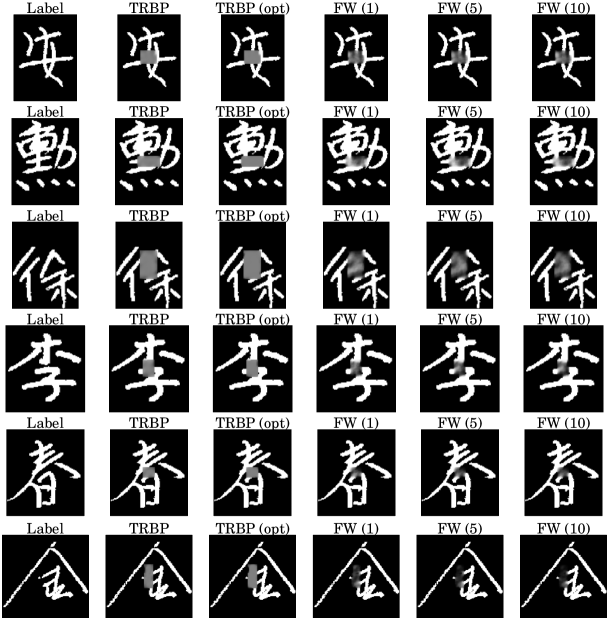
Figure 4: Chinese Characters : Additional Experiments. TRBP (opt) denotes our implementation of tightening over $\mathbb{T}$ using a wrapper over libDAI (Mooij, 2010)

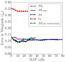
(a) $\zeta_{\mu}$: $5\times 5$ grid, $\mathcal{M}$ vs $\mathcal{M}_{\delta}$

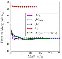
(b) $\zeta_{\mu}$: $10$ node clique, $\mathcal{M}$ vs $\mathcal{M}_{\delta}$

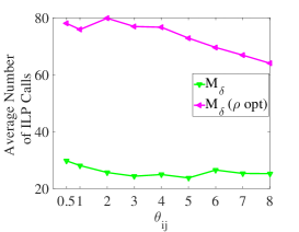
(c) Average ILP calls versus $\theta$: $10$ node clique

Figure 5: Figure 5(a), 5(b) depict $\zeta_{\mu}$ corresponding to the experimental setup in Figure 1(a), 1(b) respectively. Figure 5(c) explores the average number of ILP calls taken to convergence with and without optimizing over $\bm{\rho}$

Appendix J Bounding $\log Z$ with Approximate MAP Solvers

Suppose that we use an approximate MAP solver for line 7 of Algorithm 2. We show in this section that if the solver returns an upper bound on the value of the MAP assignment (as do branch-and-cut solvers for integer linear programs), we can use this to get an upper bound on $\log Z$. For notational consistency, we consider using Algorithm 2 for $\min_{\bm{x}\in\mathcal{D}}f(\bm{x})$, where $f(\bm{x})=-\text{TRW}(\vec{\bm{\mu}};\vec{\bm{\theta}},\bm{\rho})$ is convex, $\bm{x}=\vec{\bm{\mu}}$, and $\mathcal{D}=\mathcal{M}$.

The property that the duality gap may be used as a certificate of optimality (Jaggi, 2013) gives us:

$$f(\bm{x}^{*})\geq f(\bm{x}^{(k)})-g(\bm{x}^{(k)})\implies-f(\bm{x}^{*})\leq-f(\bm{x}^{(k)})+g(\bm{x}^{(k)}).$$ (24)

Adding the gap onto the TRW objective yields an upper bound on the optimum (which from Equation 1 is an upper bound on $\log Z$), i.e. $\log Z\leq-f(\bm{x}^{*})$. From our definition of the duality gap $g(\bm{x}^{(k)})$ (line 8 in Algorithm 2) and (24), we have:

$$\log Z\leq-f(\bm{x}^{*}) \leq-f(\bm{x}^{(k)})+\left\langle-\nabla f(\bm{x}^{(k)}),\bm{s}^{(k)}-\bm{x}^{(k)}\right\rangle$$

$$=-f(\bm{x}^{(k)})+\underbrace{\left\langle-\nabla f(\bm{x}^{(k)}),\bm{s}^{(k)}\right\rangle}_{\text{MAP call}}-\underbrace{\left\langle-\nabla f(\bm{x}^{(k)}),\bm{x}^{(k)}\right\rangle}_{\text{Can be computed efficiently}},$$

where $\bm{s}^{(k)}=\operatorname*{\arg\min}_{\bm{v}\in\mathcal{D}}\left\langle\nabla f(\bm{x}^{(k)}),\bm{v}\right\rangle=\operatorname*{\arg\max}_{\bm{v}\in\mathcal{D}}\left\langle-\nabla f(\bm{x}^{(k)}),\bm{v}\right\rangle$ (line 7 in Algorithm 2). Thus, if the approximate MAP solver returns an upper bound $\kappa$ such that $\max_{\bm{v}\in\mathcal{D}}\left\langle-\nabla f(\bm{x}^{(k)}),\bm{v}\right\rangle\leq\kappa$, then we get the following upper bound on the log-partition function:

$$\log Z\leq-f(\bm{x}^{(k)})+\kappa-\left\langle-\nabla f(\bm{x}^{(k)}),\bm{x}^{(k)}\right\rangle.$$ (25)

For example, we could use a linear programming relaxation or a message-passing algorithm based on dual decomposition such as Sontag et al. (2008) to obtain the upper bound $\kappa$. There is a subtle but important point to note about this approach. Despite the fact that we may use a relaxation of $\mathcal{M}$ such as $\mathbb{L}$ or the cycle relaxation to compute the upper bound, we evaluate it at $\vec{\bm{\mu}}^{(k)}$ that is guaranteed to be within $\mathcal{M}$. This should be contrasted to instead optimizing over a relaxation such as $\mathbb{L}$ directly with Algorithm 2. In the latter setting, the moment we move towards a fractional vertex (in line  14) we would immediately take $\vec{\bm{\mu}}^{(k+1)}$ out of $\mathcal{M}$. Because of this difference, we expect that this approach will typically result in significantly tighter upper bounds on $\log Z$. abbrvnat ref

References

• Allouche et al. (2010) D. Allouche, S. de Givry, and T. Schiex. Toulbar2, an open source exact cost function network solver, 2010.
• Andres et al. (2012) B. Andres, B. T., and J. H. Kappes. Opengm: A c++ library for discrete graphical models, June 2012.
• Belanger et al. (2013) D. Belanger, D. Sheldon, and A. McCallum. Marginal inference in MRFs using Frank-Wolfe. NIPS Workshop on Greedy Optimization, Frank-Wolfe and Friends, 2013.
• Besag (1986) J. Besag. On the statistical analysis of dirty pictures. J R Stat Soc Series B, 1986.
• Borenstein and Ullman (2002) E. Borenstein and S. Ullman. Class-specific, top-down segmentation. In ECCV, 2002.
• Boykov and Kolmogorov (2004) Y. Boykov and V. Kolmogorov. An experimental comparison of min-cut/max-flow algorithms for energy minimization in vision. TPAMI, 2004.
• Domke (2013) J. Domke. Learning graphical model parameters with approximate marginal inference. TPAMI, 2013.
• Ermon et al. (2013) S. Ermon, C. P. Gomes, A. Sabharwal, and B. Selman. Taming the Curse of Dimensionality: Discrete Integration by Hashing and Optimization. In ICML, 2013.
• Garber and Hazan (2013) D. Garber and E. Hazan. A linearly convergent conditional gradient algorithm with applications to online and stochastic optimization. arXiv preprint arXiv:1301.4666, 2013.
• Globerson and Jaakkola (2007) A. Globerson and T. Jaakkola. Convergent Propagation Algorithms via Oriented Trees. In UAI, 2007.
• Gurobi Optimization (2015) I. Gurobi Optimization. Gurobi optimizer reference manual, 2015.