Low-Thrust Lyapunov to Lyapunov and Halo to Halo Missions with $L^{2}$-Minimization

Abstract.

In this work, we develop a new method to design energy minimum low-thrust missions ($L^{2}$-minimization). In the Circular Restricted Three Body Problem, the knowledge of invariant manifolds helps us initialize an indirect method solving a transfer mission between periodic Lyapunov orbits. Indeed, using the PMP, the optimal control problem is solved using Newton-like algorithms finding the zero of a shooting function. To compute a Lyapunov to Lyapunov mission, we first compute an admissible trajectory using a heteroclinic orbit between the two periodic orbits. It is then used to initialize a multiple shooting method in order to release the constraint. We finally optimize the terminal points on the periodic orbits. Moreover, we use continuation methods on position and on thrust, in order to gain robustness. A more general Halo to Halo mission, with different energies, is computed in the last section without heteroclinic orbits but using invariant manifolds to initialize shooting methods with a similar approach.

Dans ce travail, on développe une nouvelle méthode pour construire des missions à faible poussée avec minimisation de la norme $L^{2}$ du contrôle. Dans le problème circulaire restreint des trois corps, la connaissance des variétés invariantes nous permet d’initialiser une méthode indirecte utilisée pour calculer un transfert entre orbites périodiques de Lyapunov. En effet, par l’application du Principe du Maximum de Pontryagin, on obtient la commande optimale par le calcul du zéro d’une fonction de tir, trouvé par un algorithme de Newton. Pour construire la mission Lyapunov vers Lyapunov, dans un premier temps, on calcule une trajectoire admissible en passant par une trajectoire hétérocline reliant les deux orbites périodiques. Celle-ci est alors utilisée pour initialiser un tir multiple nous permettant de relacher la contrainte de rejoindre la trajectoire hétérocline. Enfin, on optimise la position des points de départ et d’arrivée sur les orbites périodiques. De plus, pour rendre nos méthodes plus robustes, on utilise des méthodes de continuation sur la position et sur la poussée. Dans la dernière section, on contruit une mission plus générale Halo vers Halo avec des énergies différentes. Cette fois, nous ne pouvons plus utiliser d’orbites hétéroclines, mais on initialise la méthode de tir avec des trajectoires des variétés invariantes de la même façon qu’avec l’orbite hétérocline pour la mission Lyapunov vers Lyapunov.

1. Introduction

Since the late ’70s, study of libration point orbits has been of great interest. Indeed, several missions such as ISEE-3 (NASA) in 1978, SOHO (ESA-NASA) in 1996, GENESIS (NASA) in 2001, PLANK (ESA) in 2007 etc. have put this design knowledge into practice. A more profound understanding of the available mission options has also emerged due to the theoretical, analytical, and numerical advances in many aspects of libration point mission design.

There exist a huge number of references on the problem of determining low-cost trajectories by using the properties of Lagrange equilibrium points. For instance, the authors in [13, 22, 15, 40] have developed very efficient methods to find “zero cost” trajectories between libration point orbits. Dynamical system methods are used to construct heteroclinic orbits from invariant manifolds between libration point orbits and it allows to get infinite time uncontrolled transfers. These orbits have been used with impulse engines of spacecrafts to construct finite time transfers. In this work, we want to perform the transfer with a low-thrust propulsion, so impulses to reach heteroclinic orbits (or trajectories on invariant manifolds) are prohibited.

Invariant manifolds have been used in a low-thrust mission in [27, 28]. The low-thrust propulsion is introduced by means of special attainable sets that are used in conjunction with invariant manifolds to define a first-guess solution. Then, the solution is optimized using an optimal control formalism. One can note that [26] is the first work that combines invariant manifolds and low-thrust in the Earth-Moon system.

Much efforts have been dedicated to the design of efficient methods to reach periodic orbits, Halo orbits, around equilibrium points in the three body problem. For example, in [32, 29], authors use indirect methods and direct multiple shooting methods to reach an insertion point on a manifold to reach asymptotically a Halo orbit in the Earth-Moon system. Moreover, using transversality conditions, the position of the insertion point on the manifold is optimized on the manifold. Low-thrust, stable-manifold transfers to Halo orbits are also shown in [33].

On the same topic, in [26], authors use direct methods to reach a point on a stable manifold of a Halo orbit from a GTO orbit. A transfer from the Halo orbit to a Lunar-Orbit is established as well. The $L_{2}$-norm of the control is minimized by a direct transcription and non linear programming. In [24], the position of insertion point on the manifold is optimized.

We can notice that in the interesting work [9], indirect method combined with continuation methods have been used to design missions from an Earth Geostationary Orbit to a Lunar Orbit. Indeed, continuations are used from the two body problem to the three body problem, the minimum time problem is studied and solved, and continuations between energy minimization and fuel consumption minimization are computed.

Moreover, in [41], the developed methods involve the minimum-time problem, the minimum energy problem and the minimum fuel problem to reach a fixed point on a Halo orbit starting from a periodic orbit around Earth. Continuations on the thrust are used as well as Newton and bisection methods (indirect methods). In these last two contributions, manifolds are not used to help solve the formulated problem.

In [10], the author recently developed an efficient method to compute an optimal low-thrust transfer trajectory in finite time without using invariant manifolds of the three body problem. It is based on a three-step solution method using indirect methods and continuations methods and it gives good results.

The philosophy of the method developed in this work is to use the natural dynamics as invariant manifolds, providing free parts for transfer, and to initialize a global multiple shooting method freeing the constraints to stay on the manifold. The invariant manifolds are just there to help obtain convergence for a shooting method. For references on techniques used in our work such as continuation on cost, smoothing techniques, optimization techniques one may read [18, 19, 3].

To compute the required transfer with a low thrust and minimizing the energy ($L^{2}$-minimization), we will use indirect methods coming from the Pontryagin Maximum Principle [30]. Initialization of indirect methods with dynamics properties is a real challenge in order to improve the efficiency of indirect methods (see [37] and references therein). Indeed, the main difficulty of such methods is to initialize the Newton-like algorithm, and the understanding of the dynamics can be very useful to construct an admissible trajectory for the initialization. Moreover, continuation methods as used in [14] or [8], are crucial to give robustness to these indirect methods. The aim of this paper is to combine all these mathematical aspects of dynamics, optimal control and continuation methods to design low-thrust transfers between libration point orbits. Principle, we only get necessary conditions of optimality. It would be interesting to check the second order sufficient conditions, with focal point tests for example.

The outline for the article is as follows. First, in Section 2, we introduce the mission we want to perform and compute, introduce the paradigm of the Circular Restricted Three Body Problem and state our optimal control problem.

Then, in Section 3, we recall dynamical properties of the circular restricted three body problem, such as equilibrium points, Lyapunov periodic orbits, and invariant manifolds. We present the mathematical tools used to numerically compute the periodic orbits and the manifolds. In particular, we introduce in this part the continuation method that we will use throughout this article.

Then, in Section 4, we develop our method with an example mission. We first compute a heteroclinic orbit between the two Lyapunov periodic orbits. Then, fixing the departure point near $L_{1}$ and the arrival point near $L_{2}$ and with a not to small thrust ($60\text{\,}\mathrm{N}$), we perform two small transfers from the Lyapunov orbit around $L_{1}$ to the heteroclinic one, and from the heteroclinic orbit to the Lyapunov orbit around $L_{2}$. Then, thanks to a multiple shooting method we release the constraint on the position of the matching points on the heteroclinic orbit and decrease the thrust to the targeted one ($0.3\text{\,}\mathrm{N}$). Finally, we optimize the departure and arrival points on the periodic orbits to satisfy the necessary transversality conditions given by the Pontryagin Maximum Principle. In section 5.1, we present another mission with a heteroclinic orbit with two revolutions around the Moon.

Finally, in section 5.2, we apply the method to a more general mission: a Halo to Halo mission for two periodic orbits with different energies. In this case, there is no heteroclinic orbit, so we construct an admissible trajectory with 5 parts. Two of them are trajectories on invariant manifolds, and the three others are local transfers: 1/ from one of the Halo orbits to a free trajectory, 2/ between both free trajectories and 3/ from the second free trajectory to the second Halo orbit. Thanks to this five part admissible trajectory, we are able to initialize a multiple shooting method that computes an optimal trajectory (which is not constrained to reach any invariant manifolds). As previously, we optimize the terminal points on Halo orbits.

2. The Mission

2.1. Circular Restricted Three Body Problem (CRTBP)

We use the paradigm of the Circular Restricted Three Body Problem. In this section we will follow the description by [21].

Let us consider a spacecraft in the field of attraction of Earth and Moon. We consider an inertial frame $\mathcal{I}$ in which the vector differential equation for the spacecraft’s motion is written as:

$$m\dfrac{\mathrm{d}\underline{R}}{\mathrm{d}t}=-GM_{1}m\dfrac{\underline{R}_{13}}{R^{3}_{13}}-GM_{2}m\dfrac{\underline{R}_{23}}{R^{3}_{23}}$$ (1)

where $M_{1}$, $M_{2}$ and $m$ are the masses respectively of Earth, the Moon and the spacecraft, $\underline{R}$ is the spacecraft vector position, $\underline{R}_{13}$ is the vector Earth-spacecraft and $\underline{R}_{23}$ is the vector Moon-spacecraft. $G$ is the gravitational constant. Let us describe the simplified general framework we will use.

Problem Description.  To simplify the problem, and use a general framework, we consider the motion of the spacecraft $P$ of negligible mass moving under the gravitational influence of the two masses $M_{1}$ and $M_{2}$, referred to as the primary masses, or simply the primaries (here Earth and Moon). We denote these primaries by $P_{1}$ and $P_{2}$. We assume that the primaries have circular orbits around their common center of mass. The particle $P$ is free to move all around the primaries but cannot affect their motion.

The system is made adimensional by the following choice of units: the unit of mass is taken to be $M_{1}+M_{2}$; the unit of length is chosen to be the constant distance between $P_{1}$ and $P_{2}$; the unit of time is chosen such that the orbital period of $P_{1}$ and $P_{2}$ about their center of mass is $2\pi$. The universal constant of gravitation then becomes $G=1$. Conversions from units of distance, velocity and time in the unprimed, normalized system to the primed, dimensionalized system are

$$\text{distance}\quad d^{\prime}=l_{*}d,\quad\text{velocity}\quad s^{\prime}=v_{*}s,\quad\text{time}\quad t^{\prime}=\frac{t_{*}}{2\pi}t,$$ (2)

where we denote by $l_{*}$ the distance between $P_{1}$ and $P_{2}$, $v_{*}$ the orbital velocity of $P_{1}$ and $t_{*}$ the orbital period of $P_{1}$ and $P_{2}$.

We define the only parameter of this system as

$$\mu=\dfrac{M_{2}}{M_{1}+M_{2}},$$

and call it the mass parameter, assuming that $M_{1}>M_{2}$.

In table 1, we summarize the values of all the constants for the Earth-Moon CR3PB for numerical computations.

System	$\mu$	$l_{*}$	$v_{*}$	$t_{*}$
Earth-Moon	$1.215\text{\times}{10}^{-2}$	$384\,402\text{\times}{10}^{03}\text{\,}\mathrm{km}$	$1.025\text{\,}\mathrm{km}\text{\,}{\mathrm{s}}^{-1}$	$2.361\text{\times}{10}^{06}\text{\,}\mathrm{s}$

Table 1. Table of the parameter values for the Earth-Moon system.

Equations of Motion.  If we write the equations of motion in a rotating frame $\mathcal{R}$ in which the two primaries are fixed (the angular velocity is the angular velocity of their rotation around their center of mass, see [9]), we obtain that the coordinates of $P_{1}$ and $P_{2}$ are respectively $\chi_{P_{1}}=(-\mu,0,0,0,0),$ and $\chi_{P_{2}}=(1-\mu,0,0,0,0)$. Let us call $x_{1}^{0}=-\mu$ and $x_{2}^{0}=1-\mu$, and by writing the state $\chi=\left(x,y,\dot{x},\dot{y}\right)^{T}=\left(x_{1},x_{2},x_{3},x_{4}\right)^{T},$ we obtain

$$\left\{\begin{aligned} \dot{x}_{1}&=x_{3}\\ \dot{x}_{2}&=x_{4}\\ \dot{x}_{4}&=x_{1}+2x_{4}-(1-\mu)\frac{x_{1}-x_{1}^{0}}{r_{1}^{3}}-\mu\frac{x_{1}-x_{2}^{0}}{r_{2}^{3}}\\ \dot{x}_{5}&=x_{2}-2x_{3}-(1-\mu)\frac{x_{2}}{r_{1}^{3}}-\mu\frac{x_{2}}{r_{2}^{3}}\\ \end{aligned}\right.$$ (3)

where $r_{1}=\sqrt{\left(x_{1}-x_{1}^{0}\right)^{2}+x_{2}^{2}}$ and $r_{2}=\sqrt{\left(x_{1}-x_{2}^{0}\right)^{2}+x_{2}^{2}}$ are respectively the distances between $P$ and primaries $P_{1}$ and $P_{2}$.

We can define the potential $U(x_{1},x_{2})=-\frac{1}{2}\left(x_{1}^{2}+x_{2}^{2}\right)-\frac{1-\mu}{r_{1}}-\frac{\mu}{r_{2}}-\frac{1}{2}\mu\left(1-\mu\right).$ We denote by $F_{0}$ the vector field of the system and we define the energy of a state point as

$$\mathcal{E}(\chi)=\frac{1}{2}(\dot{x}^{2}+\dot{y}^{2})+U(x,y).$$ (4)

Note that the energy is constant as the system evolves over time (conservation law).

In the first part of this work, we will consider a planar motion, hence, we only have a $\mathbb{R}^{4}$-state in the orbital plane of the primaries, but this can be easily extended to the spatial case.

2.2. Design of the Transfer

We want to design a mission going from a periodic Lyapunov orbit around $L_{1}$ to a periodic Lyapunov orbit around $L_{2}$ using a low-thrust engine in the Earth-Moon system (see figure 5). A full description of these periodic orbits is given in section 3.1. In order to perform such a mission, we will use the properties introduced in section 3.3: the invariant manifolds. Indeed, if we are able to find an intersection between an “$L_{1}$ unstable manifold” and an “$L_{2}$ stable manifold”, we get an asymptotic trajectory that performs the mission with a zero thrust, called a heteroclinic orbit (see section 4.1).

In the classical literature, such a mission is usually designed by using impulse to reach the heteroclinic orbit from the Lyapunov orbit around $L_{1}$ and then another impulse to reach the Lyapunov orbit from the heteroclinic one. Since we design a low-thrust transfer, following this method is unrealistic. In [10], the author developed a three-step method to perform a low thrust low energy trajectory between Lyapunov orbits of the same energy without using invariant manifolds. At his first step, he uses a feasible quadratic-zero-quadratic control structure to initialize his method. In this work we will use the knowledge of a zero cost trajectory, the heteroclinic orbit, to initialize an indirect shooting method (Newton-like method for optimal control problem) provided by applying the Pontryagin Maximum Principle.

2.3. Controlled Dynamics

We first describe the model for the evolution of our spacecraft in the CRTBP. In non normalized coordinates (see (1)), the controlled dynamics is the $m\dfrac{\mathrm{d}\underline{R}}{\mathrm{d}t}=-GM_{1}m\dfrac{\underline{R}_{13}}{R^{3}_{13}}-GM_{2}m\dfrac{\underline{R}_{23}}{R^{3}_{23}}+T(t),$ where $T$ is the spacecraft driving force, and $m$ is the time dependant mass of the spacecraft. The equation for the evolution of the mass is

$$\dot{m}(t)=-\beta\left\|T(t)\right\|,$$

where $\beta$ is computed with the two parameters $I_{\text{sp}}$ and $g_{0}$. Specific impulse ($I_{\text{sp}}$) is a measure of the efficiency of rocket and jet engines. $g_{0}$ is the acceleration at Earth’s surface. The inverse of the average exhaust speed, $\beta$, is equal to $\frac{1}{I_{\text{sp}}g_{0}}$. Moreover, the thrust is constrained by $\left\|T(t)\right\|\leqslant T_{\text{max}}$ for all $t$.

Using the normalization parameters (2), denoting by $\beta_{*}$ the normalized parameter $\beta$ initially in $\mathrm{m}^{-1}\,\mathrm{s}$, the mass evolution is

$$\dot{m}(t)=-\beta_{*}\frac{t_{*}^{2}}{4\pi^{2}l_{*}}T_{\text{max}}\left\|u(t)\right\|$$

Moreover, we introduce the control $u$ such that $\left|u(t)\right|\leqslant 1$ and denote the normalized coefficient $\frac{t_{*}^{2}}{4\pi^{2}l_{*}}T_{\text{max}}$ by $\epsilon$.

In short, we write the system as :

$$\left\{\begin{array}[]{l}\displaystyle\dot{x}=F_{0}(x)+\frac{\epsilon}{m}\sum_{i=1}^{2}u_{i}F_{i}(x),\\ \displaystyle\dot{m}=-\beta_{*}\epsilon\left\|u\right\|,\end{array}\right.$$

where $F_{0}$ is the natural vector field defined by (3). Here we have $F_{1}(x)=\begin{pmatrix}0\\ 0\\ 1\\ 0\end{pmatrix}$, and $F_{2}(x)=\begin{pmatrix}0\\ 0\\ 0\\ 1\end{pmatrix}$. This can be easily extended to the spatial case.

Controllability.  In [6], it is proved that the CRTBP with a non evolving mass is controllable for a suitable subregion of the phase-space, denoted by $X_{\mu}^{1}$, where the energy is greater than the energy of $L_{1}$: For any $\mu\in(0,1)$, for any positive $\epsilon$, the circular restricted three-body problem is controllable on $X_{\mu}^{1}$. Using proposition (2.2) in [5], one can extend this result to the system with an evolving mass.

2.4. Optimal Control Problem (OCP)

Our main goal in this work is to solve an optimal control problem. We want to go from the Lyapunov orbit around $L_{1}$ to the Lyapunov orbit around $L_{2}$ with minimal energy. Mathematically we write this problem as follows

$$\mathcal{P}_{g}\left\{\begin{array}[]{l}\displaystyle\mathcal{C}_{g}=\min\int_{0}^{t_{f}}\left\|u\right\|^{2}\mathrm{d}t,\\ \displaystyle\dot{x}=F_{0}(x)+\frac{\epsilon}{m}\sum_{i=1}^{2}u_{i}F_{i}(x),\\ \displaystyle\dot{m}=-\beta_{*}\epsilon\left\|u\right\|,\\ \left\|u\right\|\leqslant 1,\\ x(0)\in\text{Lya}_{1},\text{ and }x(t_{f})\in\text{Lya}_{2}.\end{array}\right.$$ (5)

Let us summarize the steps in the method we developed to solve this problem :

1. First, we find a heteroclinic orbit from the Lyapunov orbit around $L_{1}$ to the Lyapunov orbit around $L_{2}$.

2. Then, we realize a short transfer from a fixed point on the Lyapunov orbit around $L_{1}$ to the heteroclinic orbit.

3. Similarly, we realize a transfer from the heteroclinic orbit to a fixed point on the Lyapunov orbit around $L_{2}$.

4. Then we release the constraint on the position of the matching connections on the heteroclinic orbit using a multiple shooting method and we decrease the maximal thrust.

5. Finally, we optimize the position of the two fixed points on $\text{Lya}_{1}$ and $\text{Lya}_{2}$ to satisfy the transversality condition for problem (5).

We note that in steps 2 to 4 (where we are solving optimal control problems), we have fixed the departure and arrival points to simplify the problem. The last step consists in releasing these constraints.

Remark: The real problem that we want to solve is the minimization of the consumption of fuel (the maximization of the final mass). This is done by considering the minimization of the $L_{1}$-norm of $u$

$$\mathcal{C}_{g}^{L_{1}}=\min\int_{0}^{t_{f}}\left\|u\right\|\mathrm{d}t.$$

Unfortunately, this implies numerical difficulties and for simplicity, we only consider here the $L_{2}$-minimization problem. One can see [9], or [41] where the authors attempt to consider the $L^{1}$-minimization. This is one of the perspective of this work using for example another continuation on the cost.

3. Properties of CRTBP

In this Section, we recall some properties of the CRTBP. In particular, we introduce equilibrium points, Lyapunov orbits and invariant manifolds. We explain how to numerically compute these orbits (see Section 3.2). We have improved the method used in [2] using the energy as continuation parameter. Finally, we introduce the invariant manifolds and how we can get a numerical approximation.

3.1. Lyapunov Orbits

Equilibrium Points.  The Lagrange points are the equilibrium points of the circular restricted three-body problem. Euler [11] and Lagrange [23] proved the existence of five equilibrium points: three collinear points on the axis joining the center of the two primaries, generally denoted by $L_{1}$, $L_{2}$ and $L_{3}$, and two equilateral points denoted by $L_{4}$ and $L_{5}$ (see figure 1).

Figure 1. Localization of Lagrange’s points.

Computing equilateral points $L_{4}$ and $L_{5}$ is not very complicated, but it is not possible to find exact solutions for collinear equilibria $L_{1}$, $L_{2}$ and $L_{3}$. We refer to [34], for series expressions. We recall that the collinear points are shown to be unstable (in every system), whereas $L_{4}$ and $L_{5}$ are proved to be stable under some conditions (see [25]).

Periodic Orbits.  The Lyapunov center theorem ensures the existence of periodic orbits around equilibrium points (see [25, 4] and references therein). To use this theorem, one has to linearize the system and compute the eigenvalues of the linearized system.

In the planar case, applying this theorem to the collinear points $L_{1}$, $L_{2}$ and $L_{3}$ we get a one-parameter family of periodic orbits around each one. These periodic orbits are called Lyapunov orbits and are homeomorphic to a circle. In this work, we denote by $\text{Lya}_{i}$ a Lyapunov orbit around the equilibrium point $L_{i}$. For the spatial case, periodic orbits are called Halo orbits or Lissajous orbits (see e.g. [16]).

Numerical computation.  We will describe the method to compute Lyapunov orbits around collinear Lagrange points. For the spatial case we follow the same method. To find these periodic orbits, we use a Newton-like method. Since equations in the coordinate system centered on $L_{i}$ are symmetric, if we consider a periodic solution $\chi(t)=(x(t),y(t),\dot{x}(t),\dot{y}(t))$ of period $t_{\chi}$, then there exists $t_{0}$ such that

$$\left\{\begin{array}[]{l}x(t_{0})=x_{0},\\ y(t_{0})=0,\\ \dot{x}(t_{0})=0,\\ \dot{y}(t_{0})=\dot{y}_{0},\end{array}\right.\text{ and }\left\{\begin{array}[]{l}x(t_{0}+t_{\chi}/2)=x_{1},\\ y(t_{0}+t_{\chi}/2)=0,\\ \dot{x}(t_{0}+t_{\chi}/2)=0,\\ \dot{y}(t_{0}+t_{\chi}/2)=\dot{y}_{1}.\end{array}\right.$$

Since $t_{0}$ could be chosen to be equal to zero and fixing $x_{0}$, we just have to find $(\dot{y}_{0},t_{\chi})$ such that, denoting by $\phi$ the flow of the dynamical system, and $\chi_{0}=(x_{0},0,0,\dot{y}_{0})$, the function $\mathcal{S}_{L}$ satisfies:

$$\mathcal{S}_{L}(t_{\chi},\dot{y}_{0})=\begin{pmatrix}\phi_{2}(t_{\chi}/2,\chi_{0})\\ \phi_{3}(t_{\chi}/2,\chi_{0})\end{pmatrix}=\begin{pmatrix}0\\ 0\end{pmatrix}.$$ (6)

In practice, we fix for example the value of $x_{0}$ (respectively of $z_{0}$ in the spatial case) in order to be left with finding a zero of a function of two variables $(\dot{y}_{0},t_{\chi})$ in $\mathbb{R}^{2}$ . Obviously, we can extend this to a periodic orbit in $\mathbb{R}^{6}$.

The main difficulty is to initialize the Newton-like algorithm. The idea is to find an analytical approximation of the orbit to a certain order, and then inject this into the Newton-like algorithm. In this work, and because the Lyapunov orbit is not very difficult to compute, we follow [31]. For various orbits in $\mathbb{R}^{6}$, see [2, 20, 12] and references therein.

3.2. Computing the family

In order to use these orbits to construct the targeted mission, it is very useful to be able to compute the family of periodic orbits, providing us with different orbits that have different energies.

3.2.1. Continuation methods

To explain how we get the family of periodic orbits, let us introduce continuation methods, for a more complete introduction, see [1]. The main idea is to construct a family of problems denoted by $\left(\mathcal{P}_{\lambda}\right)_{\lambda\in[0,1]}$ indexed by a parameter $\lambda\in[0,1]$. The initial problem $\mathcal{P}_{0}$ is supposed to be easy to solve, and the final problem $\mathcal{P}_{1}$ is the one we want to solve.

Let us assume that we have solved numerically $\mathcal{P}_{0}$, and consider a subdivision $0=\lambda_{0}<\lambda_{1}<\cdots<\lambda_{p}=1$ of the interval $[0,1]$. The solution of $\mathcal{P}_{0}$ can be used to initialize the Newton-like method applied to $\mathcal{P}_{\lambda_{1}}$. And so on, step by step, we use the solution of $\mathcal{P}_{\lambda_{i-1}}$ to initialize $\mathcal{P}_{\lambda_{i}}$. Of course, the sequence $\left(\lambda_{i}\right)$ has to be well chosen and eventually should be refined.

Mathematically, for this method to converge, we need that the family of problems to depend continuously on the parameter $\lambda$. See [4, chap. 9] for some justification of the method.

From the numerical point of view, there exist many methods and strategies for implementing continuation or homotopy methods. We can distinguish between differential pathfollowing, simplicial methods, predictor-corrector methods, etc. In this work, we implement a predictor-corrector method because it is suitable for our problem. Here, we use a “constant” prediction: the solution of problem $\mathcal{P}_{\lambda_{i-1}}$ is used to initialized the resolution of problem $\mathcal{P}_{\lambda_{i}}$. We can note that there exist many codes which can be found on the web, such as the well-known Hompack90 [39] or Hampath [8]. For a survey about different results, challenges and issues on continuation methods, see [37].

3.2.2. Application to the family of orbits

Since we had to choose a parameter $x_{0}$ to write the zero function $\mathcal{S}_{L}$ in (6), it is natural to use this parameter to perform the continuation that computes the family of orbits. Indeed, we can choose to reach a certain $x_{0}^{\text{obj}}$ (respectively a so called excursion $z_{0}^{\text{obj}}$ in the spatial case). So we can define our continuation as :

$$\mathcal{P}_{\lambda}:\left\{\begin{array}[]{l}\text{for }x_{0}^{\lambda}=(1-\lambda)x_{0}+\lambda x_{0}^{\text{obj}}\\ \mathcal{S}_{L}^{\lambda}(t_{\chi},\dot{y}_{0})=\begin{pmatrix}\phi_{2}(t_{\chi}/2,\chi_{0}^{\lambda})\\ \phi_{3}(t_{\chi}/2,\chi_{0}^{\lambda})\end{pmatrix}=\begin{pmatrix}0\\ 0\end{pmatrix}\end{array}\right.$$

where $\chi_{0}^{\lambda}=(x_{0}^{\lambda},0,0,\dot{y}_{0})$. Thanks to the analytical approximation provided by [31] or [20], we can solve the initial problem $\mathcal{P}_{0}$. We can note that such analytical approximation does not work for every $x_{0}$. Using the continuation method described previously, we can get a family of periodic orbit.

However, for some periodic orbits (Halo family), we can observe that the continuation fails when we converge to the equilibrium point ($x_{0}^{\text{obj}}\to 0$). A much better continuation parameter is energy. It releases the constraint on the parameter $x_{0}$, and allows us to reach any periodic orbit, in particular the algorithm converges to the energy of $L_{i}$, $i\in\{1,\dots,3\}$. Moreover, it is a significantly more natural parameter, keeping in mind the fact that we will construct a controlled transfer method. Section 3.3 will provide an extra argument in favor of the energy parameter. It seems to be the first time that this continuation is done with the energy as the continuation parameter. This avoids numerical problems when reaching energy close to $L_{i}$.

Thanks to the analytical approximation, we get a first periodic orbit with energy $\mathcal{E}_{0}$, and we want to reach a prescribed energy $\mathcal{E}_{1}$ so we define the following family of problems:

$$\mathcal{P}_{\lambda}^{\mathcal{E}}:\begin{array}[]{l}\mathcal{S}_{\mathcal{E}}^{\lambda}(t_{\chi},x_{0},\dot{y}_{0})=\begin{pmatrix}\phi_{2}(t_{\chi}/2,\chi_{0})\\ \phi_{3}(t_{\chi}/2,\chi_{0})\\ \mathcal{E}(\chi_{0})-\mathcal{E}_{\lambda}\end{pmatrix}=\begin{pmatrix}0\\ 0\\ 0\end{pmatrix}\end{array}$$

where $\mathcal{E}(\chi_{0})$ is the energy of the trajectory starting at $\chi_{0}$ and $\mathcal{E}_{\lambda}=(1-\lambda)\mathcal{E}_{0}+\lambda\mathcal{E}_{1}$.

In the continuation, we just use a predictor-corrector continuation with a “constant” prediction as explain before (see [1]). If necessary, one could improve this by using a linear predictor continuation, but using energy as a continuation parameter, continuation was very fast and easy, and did not require improvements.

Figure 2 shows an example of a family of Lyapunov orbits around $L_{1}$ in the Earth-Moon system.

Figure 2. A family of Lyapunov orbits around $L_{1}$ in the Earth-Moon system (Richardson coordinates)

3.3. Invariant Manifolds

All the periodic orbits described in the previous section come with their invariant manifolds, that is to say, the sets of phase points from which the trajectory converges to the periodic orbit, forward for the stable manifold and backward for the unstable manifold. These manifolds can be very useful to design interplanetary missions because as separatrix, they are some sort of gravitational currents. We refer to [21, chap. 4] for the proof of existence and a more detailed explanation of these manifolds. For the sake of numerical reproducibility, we recall some well known properties.

Monodromy Matrix.  We introduce a tool of dynamical systems: the monodromy matrix. Some properties of this matrix are needed to numerically compute the invariant manifolds. For more details, see [25, 21].

Let $\bar{x}(\cdot)$ be a periodic solution of the dynamical system with period $T$ and $\bar{x}(0)=\bar{x}_{0}$. Denoting by $\phi$ the flow of the system, the monodromy matrix $M$ of the periodic orbit for the point $\bar{x}_{0}$ is defined as

$$M=\dfrac{\partial\phi(T;\bar{x}_{0})}{\partial x_{0}}.$$

It determines whether initial perturbations $\delta\bar{x}_{0}$ of the periodic orbit decay or grow.

Local Approximation to Compute Invariant Manifolds.  Using the Poincaré map we can show that the eigenvectors corresponding to eigenvalues of the monodromy matrix are linear approximations of the invariant manifolds of the periodic orbit. For the planar Lyapunov orbits in the CRTBP, we show that the four eigenvalues of $M$ are $\lambda_{1}>1,\quad\lambda_{2}=\frac{1}{\lambda_{1}},\quad\lambda_{3}=\lambda_{4}=1.$ The eigenvector associated with eigenvalue $\lambda_{1}$ is in the unstable direction and the eigenvector associated with eigenvalue $\lambda_{2}$ is in the stable direction.

Then, the method to compute invariant manifolds is the following:

1. First, for $\chi_{0}$ a point on the periodic orbit, we compute the monodromy matrix and its eigenvectors. Let us denote by $Y^{s}(\chi_{0})$ the normalized stable eigenvector and by $Y^{u}(\chi_{0})$ the normalized unstable eigenvector.

2. Then, let

   $$\begin{array}[]{l}\chi^{s\pm}(\chi_{0})=\chi_{0}\pm\alpha Y^{s}(\chi_{0}),\\ \chi^{u\pm}(\chi_{0})=\chi_{0}\pm\alpha Y^{u}(\chi_{0}),\end{array}$$ (7)

   be the initial guesses for (respectively) the stable and unstable manifolds. The magnitude of $\alpha$ should be small enough to be within the validity of the linear estimate but not too small to keep a reasonable time of escape or convergence (for instance, see [17] for a discussion on the value of $\alpha$).

3. Finally, we integrate numerically the unstable vector forward in time, using both $\alpha$ and $-\alpha$ to generate the two branches of the unstable manifold denoted by $W^{u\pm}(\chi_{0})$. We do the same for the stable vector backwards, and we get the two branches of stable manifold $W^{s\pm}(\chi_{0})$ (see figure 3).

Figure 3. Illustration of the method to compute invariant manifolds.

Following this process, we are able to compute the invariant manifolds of any Lyapunov orbit at any energy (greater than the energy of $L_{i}$, for an explanation of that, see the section about Hill regions in [21]). We have represented parts of these manifold for a Lyapunov orbit in the Earth-Moon system at energy $-1.59208$ in normalized coordinates in figure 4. Note that an interesting study of fast numerical approximation of invariant manifolds can be found in [35].

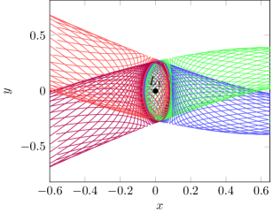
Figure 4. Manifolds of a Lyapunov orbit around $L_{1}$ of the Earth-Moon system and Richardson coordinates. The energy of these orbit and manifolds is $-1.59208$ in normalized coordinates (centered on the barycenter of the two primaries).

Remark: Since we are following invariant manifolds converging in infinite time to the periodic orbits (backward or forward), and because we are doing it numerically and so with a certain approximation, there exist long times for which we cannot obtain convergence. We have to tune the parameter $\alpha$ in (7) (we give in section 4.1 the choice of the numerical value). Moreover, the multiple shooting method allows subdividing the time and keep each part to a reasonable time of integration.

4. Constructing the Mission

In this section we explain all the steps of our method for solving the problem (5). We first find a heteroclinic orbit between the two Lyapunov orbits. Then we perform two short transfers from $\text{Lya}_{1}$ to the heteroclinic orbit, and from the heteroclinic orbit to $\text{Lya}_{2}$. Then, with a multiple shooting method we release the constraint on the position of the matching connections on the heteroclinic orbit. Finally, we optimize the departure and arrival points previously fixed to simplify the problem.

4.1. The Heteroclinic Orbit

Let us first find the heteroclinic orbit between a Lyapunov orbit around $L_{1}$ and a Lyapunov orbit around $L_{2}$. One condition to be able to find such an orbit is to compute an intersection between two manifolds. Hence, these two manifolds should have the same energy. Since the manifold and the Lyapunov orbit have the same energy, we must compute two Lyapunov orbits around $L_{1}$ and $L_{2}$ with a given energy.

The study of the well known Hill regions (see [21] and references therein), i.e. the projection of the energy surface of the uncontrolled dynamics onto the position space gives us an indication of the interval of energy we can use. Indeed, we have to compute an orbit with an energy greater than the $L_{2}$ energy. And because we want to realize a low-thrust transfer, we choose to keep a low energy. Moreover, we have a smaller region of possible motion, and so, a possibly shorter transfer.

Using the method described in 3.2.2, we choose to get two orbits with an energy of $-1.592081$ in the normalized system.

Finding the intersection.  To find an intersection, we introduce two 2D sections $U_{2}=\{(x,y)\in\mathbb{R}^{2},\;x=1-\mu,\;y<0\},$ and $U_{3}=\{(x,y)\in\mathbb{R}^{2},\;x=1-\mu,\;y>0\}$. We represent them in figure 5.

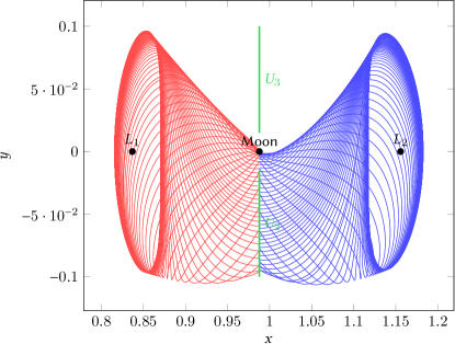
Figure 5. On the left: Planes $U_{2}$ and $U_{3}$ in the Earth-Moon system. On the right, unstable (red) and stable (blue) manifolds respectively from $L_{1}$ and $L_{2}$ stopping at the plane $U_{2}$

Then, we compute the intersection of the unstable manifold from $L_{1}$ and the stable manifold from $L_{2}$ with the space $U_{2}$ (of course, we can do the symmetric counterpart: stable manifold from $L_{1}$ and unstable manifold from $L_{2}$ with the space $U_{3}$). Since the $x$-coordinate is fixed by $U_{2}$ and because the energies of the two manifolds are equal, we just have to compute the intersection in the $(y,\dot{y})$-plan (values of $\dot{x}$ are deduced from the energy equation (4)).

We show in figure 6 the $U_{2}$-section and the existence of intersections for our particular energy. To find precisely one intersection point, we have used once more a Newton-like method. We can parametrize the section of one manifold with $U_{2}$ with only one parameter, the parameter of the Lyapunov orbit. We denote by $\phi^{+}_{x=1-\mu}$, the flow propagating forward a state point from $\text{Lya}_{1}$ onto the space $U_{2}$, and by $\phi^{-}_{x=1-\mu}$ the flow propagating backward a state point from $\text{Lya}_{2}$ onto the plan $U_{2}$. Time of propagation is fixed by the condition $x=1-\mu$.

We want to find two points $\chi_{L_{1}}\in\text{Lya}_{1}$ and $\chi_{L_{2}}\in\text{Lya}_{2}$ such that

$$\phi^{+}_{x=1-\mu}(\chi^{u+}(\chi_{L_{1}}))-\phi^{-}_{x=1-\mu}(\chi^{s-}(\chi_{L_{2}}))=0,$$

where $\chi^{u+}$ and $\chi^{s-}$ are defined in (7). This is an equality in $\mathbb{R}^{2}$, and because each of the Lyapunov orbits is parametrized with a one dimensional parameter (the time), our problem is well posed.

To initialize the method we use a discretisation (100 points in this particular example) of the Lyapunov orbits and we take the two points minimizing the Euclidean norm in the $U_{2}$ section.

Figure 6. Section in the plane $U_{2}$ of a unstable manifold from $L1$ and a stable manifold from $L_{2}$. The energy is $-1.592081$. On the right, a zoom on the interesting area.

In our case, with a value of energy equal to $-1.592081$ and $\alpha=\frac{1}{384402}$ from (7), we obtain the heteroclinic trajectory represented in figure 7. From now on, we will denote this heteroclinic orbit by Het. Note that this computation only takes few seconds on a standard desktop computer.

Figure 7. Heteroclinic orbit between two Lyapunov orbits in the Earth-Moon system. We get a travel time of $8.9613933501964$ (normalized time) or $38.974$ days.

4.2. From One Orbit to Another

Here, we construct two rather simple problems: first we compute an optimal control using the Pontryagin Maximum Principle reaching the heteroclinic orbit from the Lyapunov orbit around $L_{1}$, then we compute an optimal control to reach the Lyapunov orbit around $L_{2}$ from the heteroclinic orbit. This way, we get an admissible control that follows the null control heteroclinic orbit during a certain time.

4.2.1. Around $L_{1}$

Problem Statement.  Consider two points $\chi_{0}^{*}\in\text{Lya}_{1}$ and $\chi_{1}^{*}\in\text{Het}$, a time $t_{0}$ and an initial mass $m_{0}^{*}=$1500\text{\,}\mathrm{k}\mathrm{g}$$. We apply the Pontryagin Maximum Principle to the following problem:

$$\mathcal{P}_{L_{1}}\left\{\begin{array}[]{l}\displaystyle\min\int_{0}^{t_{0}}\left\|u\right\|^{2}\mathrm{d}t,\\ \displaystyle\dot{x}=F_{0}(x)+\frac{\epsilon}{m}\sum_{i=1}^{2}u_{i}F_{i}(x),\\ \displaystyle\dot{m}=-\beta_{*}\epsilon\left\|u\right\|,\\ \left\|u\right\|\leqslant 1,\\ x(0)=\chi_{0}^{*},\;m(0)=m_{0}^{*}\text{ and }x(t_{0})=\chi_{1}^{*}.\end{array}\right.$$ (8)

Here, we have fixed the two points $\chi_{0}^{*}$ and $\chi_{1}^{*}$ on the Lyapunov orbit and the heteroclinic orbit. We will see how we choose these points later. We will release the constraint on the position of these two points by an optimization and satisfy the transversality conditions for problem 5 in the last steps of our method.

Since the two points $\chi_{0}^{*}$ and $\chi_{1}^{*}$ belong to trajectories with an energy greater than $\mathcal{E}(L_{2})>\mathcal{E}(L_{1})$, we know that an admissible trajectory connecting $\chi_{0}^{*}$ to $\chi_{1}^{*}$ exists (see [9]).

If $t_{0}$ is greater than the minimum time, we can show that we are in the normal case for the Pontryagin Maximum Principle, that is to say $p^{0}$ can be normalized to $-1$ (see proposition 2 in [6]). Although we have not proved that this assumption holds, we will see that it is a reasonable one because of the construction of our two points. Moreover, because normality of the trajectories relies on the invariance of the target with respect to the zero control (see [14] and [7]), the normality property holds for the targeted problem (5).

We define the Hamiltonian as $\mathcal{H}(x,m,p,p_{m},u)=-\left\|u\right\|^{2}+\langle p,\;F(x)\rangle-\langle p_{m},\;\beta_{*}\epsilon\left\|u\right\|\rangle,$ where $F(x)=F_{0}(x)+\frac{\epsilon}{m}\sum_{i=1}^{2}u_{i}F_{i}(x)$, $p\in\mathbb{R}^{4}$ and $p_{m}\in\mathbb{R}$.

To simplify the notation, we write:

$$\mathcal{H}(x,m,p,p_{m},u)=-\left\|u\right\|^{2}+H_{0}+H_{1}+H_{2}-\langle p_{m},\;\beta_{*}\epsilon\left\|u\right\|\rangle,$$

where $H_{i}=\langle p,\;F_{i}(x)\rangle$, $i=0,\dots,2$.

Let us define $\varphi(p)=(p_{3},p_{4})$, thanks to the maximization condition of the Pontryagin Maximum Principle, we get the optimal control. Denoting by $y=(x,m,p,p_{m})$, let us introduce the switching function:

$$\psi(y)=\frac{-\beta_{*}\epsilon p_{m}-\epsilon/m\left\|\varphi(p)\right\|}{2}.$$

Then, the control is:

• if $\left\|\varphi(p)\right\|\neq 0$, then

  $$\left\{\begin{array}[]{ll}u(y)=0&\text{ if $\psi(y)\leqslant 0$},\\ u(y)=\psi(y)\frac{\varphi(p)}{\left\|\varphi(p)\right\|}&\text{ if $\psi(y)\in[0,1]$},\\ u(y)=\frac{\varphi(p)}{\left\|\varphi(p)\right\|}&\text{ else},\\ \end{array}\right.$$

• if $\left|\varphi(p)\right|=0$, then

  $$\left\{\begin{array}[]{ll}u(y)=0&\text{ if $\psi(y)\leqslant 0$},\\ u(y)\in\mathbf{S}(0,\psi(y))&\text{ if $\psi(y)\in[0,1]$},\\ u(y)\in\mathbf{S}(0,1)&\text{ else},\\ \end{array}\right.$$

  where $\mathbf{S}(a,b)$ is the $\mathbb{R}^{2}$-sphere centered in $a$ with radius $b$. We will not take into account the singularity $\varphi(p)=0$. Hence, the control is continuous. This is one of the reasons why the numerical methods are easier for the minimization of the $L_{2}$-norm of $u$ than for the minimization of the $L_{1}$-norm.

In this problem, let us write the transversality conditions from the Pontryagin Maximum Principle for the first problem (8). The free mass at the end of the transfer gives us : $p_{m}(t_{0})=0$. Moreover, because of the final condition $x(t_{0})=\chi_{1}^{*}$, $p(t_{0})$ is free. Finally, we are left to find $(p(0),p_{m}(0))$ such that the final state condition is satisfied.

We can write this problem as a shooting function. We denote by $\phi^{\text{ext}}$ the extremal flow of the extremal system. Hence, we define the shooting function:

$$\mathcal{S}_{L_{1}}(p(0),p_{m}(0))=\begin{pmatrix}\phi^{\text{ext}}_{1,\dots,4}(\chi_{0}^{*},m_{0}^{*},p(0),p_{m}(0))-\chi_{1}\\[5.0pt] \phi^{\text{ext}}_{10}(\chi_{0}^{*},m_{0}^{*},p(0),p_{m}(0))\end{pmatrix}=\begin{pmatrix}\underline{0}\\[5.0pt] 0\end{pmatrix}.$$ (9)

We compute the solution, that is to say $p(0)$ and $p_{m}(0)$ using a shooting method (Newton-like method applied to (9)). As is well known, the main difficulty is to initialize the Newton-like algorithm. To do this, we have used a continuation method. Let us explain the process.

Construction of $\chi_{0}^{*}$ and $\chi_{1}^{*}$.  We want to realize the transfer from $\text{Lya}_{1}$ to Het and we have already computed the heteroclinic orbit. The method is the following:

1. If we denote by $\chi_{\text{Het}}^{L_{1}}$ the first point of the “numerical” heteroclinic orbit near the Lypunov orbit, we find $\chi_{\text{Lya}_{1}}\in\text{Lya}_{1}$ by minimizing the euclidean norm : $\chi_{\text{Lya}_{1}}=\operatorname*{arg\,min}_{\chi\in\text{Lya}_{1}}\left\|\chi_{\text{Het}}^{L_{1}}-\chi\right\|$.

2. Then, we propagate backward in time $\chi_{\text{Lya}_{1}}$ following the uncontrolled dynamics during a time $t_{\text{Lya}_{1}}$ (smaller than the period of the Lyapunov orbit) to get $\chi_{0}^{*}$

3. We propagate forward in time $\chi_{\text{Het}}^{L_{1}}$ during a reasonable time $t_{\text{Het}}^{L_{1}}$ to get $\chi_{1}^{*}$ (small compared to the traveling time to reach the other extremity of Het).

We define the transfer time $t_{0}$ in (8) as $t_{0}=t_{\text{Lya}_{1}}+t_{\text{Het}}^{L_{1}}.$

Although it seems to be a more simple problem than problem (5), the main difficulty is still to initialize the shooting method. We use a continuation method on the final state, using as a first simpler problem a natural trajectory corresponding to a null control. Then step by step, we reach the targeted final point on the heteroclinic orbit, as explained next.

Final State Continuation.  As explained in section 3.2.1, we construct a family of problems $\mathcal{P}_{\lambda}$ depending continuously on one parameter $\lambda$ such that $\mathcal{P}_{0}$ is easy to solve and $\mathcal{P}_{1}$ corresponds to the targeted problem, that is to say (8).

First, let us define $\chi_{\text{Lya}_{1}}^{\text{nat}}$ as the forward propagation of $\chi_{\text{Lya}_{1}}$ following the uncontrolled dynamics during time $t_{0}$. Then we define the family of problems:

$$\mathcal{P}_{L_{1}}^{\lambda}\left\{\begin{array}[]{l}\displaystyle\min\int_{0}^{t_{0}}\left\|u\right\|^{2}\mathrm{d}t,\\ \displaystyle\dot{x}=F_{0}(x)+\frac{\epsilon}{m}\sum_{i=1}^{2}u_{i}F_{i}(x),\\ \displaystyle\dot{m}=-\beta_{*}\epsilon\left\|u\right\|,\\ \left\|u\right\|\leqslant 1,\\ x(0)=\chi_{0}^{*},\;m(0)=m_{0}^{*},\\[3.0pt] x(t_{0})=(1-\lambda)\chi_{\text{Lya}_{1}}^{\text{nat}}+\lambda\chi_{1}^{*}.\end{array}\right.$$

Figure 8. All relevant points in the construction of the problem.

Since $\chi_{\text{Lya}_{1}}^{\text{nat}}$ corresponds to the uncontrolled dynamics, the corresponding initial costate $(p(0),p_{m}(0))$ is zero. Then, step by step, we initialize the shooting method of $\mathcal{P}_{L_{1}}^{\lambda_{i}}$ using the solution of $\mathcal{P}_{L_{1}}^{\lambda_{i-1}}$ to reach problem (8). This is done by a linear prediction, e.i., the solution of the two previous iterations of the continuation are used to initialize the resolution of the next step by a linear prediction.

Figure 8 shows the different points defined for some parameters described below.

Numerical Results.  We show here the numerical results for this transfer. We choose a maximal thrust equal to $60\text{\,}\mathrm{N}$. We postpone to section 4.3 the problem of the maximum thrust which should be very small. In fact, a high thrust implies that the magnitude of the costate stays very low, and it will be necessary for the multiple shooting to converge. Indeed, for a non-saturating control, the higher the maximal magnitude of the thrust, the lower the control $u$ is between $[0,1]$, and so the lower the magnitude of $\psi(y)$ and thus of the costate. Moreover, we choose the two times of propagation in the normalized system as $t_{\text{Lya}_{1}}=1.0$, and $t_{\text{Het}}^{L_{1}}=2.0.$

We obtain the optimal trajectory plotted in figure 8. The optimal command is shown in figure 9. One can see that we are far from the saturation of the command, indeed, the maximum value is approximately $\mathrm{6}\mathrm{e}\mathrm{-}\mathrm{0}\mathrm{6}$, whereas we are constrained by one. We postpone the discussion on the real value in Newton to the final trajectory.

Figure 9. Command to realize the optimal transfer from the Lyapunov orbit to the heteroclinic orbit. We plot $u(\cdot)\leqslant 1$ as a function of the normalized time.

This continuation gives us an initial adjoint vector (costate) that we will denote by $p_{0}^{*}$ and $p_{m}^{0*}$ in the remainder of this work.

4.2.2. Around $L_{2}$

We design a very similar problem around $L_{2}$.

Problem Statement.  Consider two points $\chi_{2}^{*}\in\text{Het}$ and $\chi_{3}^{*}\in\text{Lya}_{2}$, a time $t_{2}$ and an initial mass $m_{2}^{*}$. The mass $m_{2}^{*}$ is the final mass obtained after solving for the transfer around $L_{1}$ (between the two problem we follow a heteroclinic orbit without any fuel consumption). We apply the Pontryagin Maximum Principle to the following problem:

$$\mathcal{P}_{L_{2}}\left\{\begin{array}[]{l}\displaystyle\min\int_{0}^{t_{2}}\left\|u\right\|^{2}\mathrm{d}t,\\ \displaystyle\dot{x}=F_{0}(x)+\frac{\epsilon}{m}\sum_{i=1}^{2}u_{i}F_{i}(x),\\ \displaystyle\dot{m}=-\beta_{*}\epsilon\left\|u\right\|,\\ \left\|u\right\|\leqslant 1,\\ x(0)=\chi_{2}^{*},\;m(0)=m_{2}^{*}\text{ and }x(t_{2})=\chi_{3}^{*}.\end{array}\right.$$ (10)

As before, we have fixed $\chi_{2}^{*}$ and $\chi_{3}^{*}$ on the heteroclinic and Lyapunov orbits. The final steps will allow us to release these constraints.

Since the problem is very similar to the problem around $L_{1}$, we have the same Hamiltonian and the same expression of the control $u$. Hence, we get the following shooting function:

$$\mathcal{S}_{L_{2}}(p(0),p_{m}(0))=\begin{pmatrix}\phi^{\text{ext}}_{1,\dots,4}(\chi_{2}^{*},m_{2}^{*},p(0),p_{m}(0))-\chi_{3}^{*}\\[5.0pt] \phi^{\text{ext}}_{10}(\chi_{2}^{*},m_{2}^{*},p(0),p_{m}(0))\end{pmatrix}=\begin{pmatrix}\underline{0}\\[5.0pt] 0\end{pmatrix}.$$

Construction of $\chi_{2}^{*}$ and $\chi_{3}^{*}$.  We construct the two points following the same method.

1. If we denote by $\chi_{\text{Het}}^{L_{2}}$ the last point of the heteroclinic orbit near the Lyapunov orbit, we find $\chi_{\text{Lya}_{2}}\in\text{Lya}_{2}$ minimizing the euclidean norm : $\chi_{\text{Lya}_{2}}=\operatorname*{arg\,min}_{\chi\in\text{Lya}_{2}}\left\|\chi_{\text{Het}}^{L_{2}}-\chi\right\|$.

2. Then, we propagate forward $\chi_{\text{Lya}_{2}}$ following the uncontrolled dynamics during a time $t_{\text{Lya}_{2}}$ (smaller than the period of Lyapunov orbit) to get $\chi_{3}^{*}$.

3. We propagate backward the $\chi_{\text{Het}}^{L_{2}}$ during a reasonable time $t_{\text{Het}}^{L_{2}}$ to get $\chi_{2}^{*}$ (small compared to the traveling time to reach the other extremity).

We define the transfer time $t_{2}$ in (10) as $t_{2}=t_{\text{Lya}_{2}}+t_{\text{Het}}^{L_{2}}.$

Final State Continuation.  As before, we construct a family of problems $\mathcal{P}_{\lambda}$ depending continuously on one parameter $\lambda$ such that $\mathcal{P}_{0}$ is easy to solve and $\mathcal{P}_{1}$ corresponds to the targeted problem, that is to say (8).

First, let us define $\chi_{\text{Het}}^{\text{nat}}$ as the forward propagation of $\chi_{\text{Het}}$ following the uncontrolled dynamics during the time $t_{2}$. Then we define the family of problems:

$$\mathcal{P}_{L_{2}}^{\lambda}\left\{\begin{array}[]{l}\displaystyle\min\int_{0}^{t_{2}}\left\|u\right\|^{2}\mathrm{d}t,\\ \displaystyle\dot{x}=F_{0}(x)+\frac{\epsilon}{m}\sum_{i=1}^{2}u_{i}F_{i}(x),\\ \displaystyle\dot{m}=-\beta_{*}\epsilon\left\|u\right\|,\\ \left\|u\right\|\leqslant 1,\\ x(0)=\chi_{2}^{*},\;m(0)=m_{2}^{*},\\[3.0pt] x(t_{2})=(1-\lambda)\chi_{\text{Het}}^{\text{nat}}+\lambda\chi_{3}^{*}.\end{array}\right.$$

Numerical Results.  As before, we set $T_{\text{max}}=$60\text{\,}\mathrm{N}$$, and we compute the continuation for the two times chosen as $t_{\text{Het}}^{L_{2}}=2.0,$ and $t_{\text{Lya}_{2}}=1.0$.

Figure 10 shows the optimal control to realize the final transfer from the heteroclinic orbit to the Lyapunov one around $L_{2}$. We see that, once again, we are far from the saturation of $u$.

Figure 10. Command to realize the optimal transfer from the Lyapunov orbit to the heteroclinic orbit. We plot $u(\cdot)\leqslant 1$ as a function of the normalized time.

This continuation gives us an initial costate that we will denote by $p_{2}^{*}$ and $p_{m}^{2*}$ in the remainder of this work.

Table 2 sums up all the parameters for the continuation computation. We observe that, because we are using indirect shooting methods, the computation is very fast even though it is performed on a simple desktop computer or on a single-board computer (the Raspberry Pi).

$I_{\text{sp}}$	$g_{0}$	Earth Mass	Moon Mass	Distance	Period
$2000\text{\,}\mathrm{s}$	$9.8\text{\,}\mathrm{m}^{3}\mathrm{k}\mathrm{g}^{-1}\mathrm{s}^{-2}$	$5.972\text{\times}{10}^{24}\text{\,}\mathrm{k}\mathrm{g}$	$7.349\text{\times}{10}^{22}\text{\,}\mathrm{k}\mathrm{g}$	$384\,402\text{\times}{10}^{3}\text{\,}\mathrm{m}$	$2.361\text{\times}{10}^{6}\text{\,}\mathrm{s}$

Transfer	Iterations	Cost	$T_{\text{max}}$
$L_{1}$	21	$6.309\,67\text{\times}{10}^{-11}$	$60\text{\,}\mathrm{N}$
$L_{2}$	19	$9.061\,24\text{\times}{10}^{-10}$	$60\text{\,}\mathrm{N}$

System	Transfer	Execution time
Core i7	$L_{1}$	98% cpu 2,821s total
	$L_{2}$	96% cpu 1,439s total
Raspberry Pi A	$L_{1}$	38% cpu 8,009s total
	$L_{2}$	22% cpu 7,879s total

Table 2. Numerical results for the two transfers around $L_{1}$ and $L_{2}$. Computations are performed on a simple laptop Core i7, and on a Raspberry Pi A, a credit card-sized single-board computer.

4.3. Multiple Shooting

Thanks to the results from previous sections, we have designed an admissible control to perform the transfer from a Lyapunov orbit around $L_{1}$ to a Lyapunov orbit around $L_{2}$. We first reach a point on a heteroclinic orbit, then we follow the natural dynamics (null control), and finally reach a point on the final Lyapunov orbit from a certain point on the heteroclinic orbit. This admissible trajectory is however not energy optimal, since the stay on the heteroclinic orbit is forced.

These two points on the heteroclinic orbit were arbitrarily chosen. There is no guarantee that they provide a good choice in terms of optimality. Hence, we want to release the constraints on the position of these two points. We use a multiple shooting method on top of the first two local transfer to get a better optimum.

Figure 11. Admissible trajectory in three parts.

Let us describe how we state the multiple shooting problem. As we can see in figure 11, there are two points $\chi_{1}^{*}$ and $\chi_{2}^{*}$ belonging to the heteroclinic orbit that we want to free. Moreover, we have three times:

• $t_{0}$ which is the time defined for the transfer around $L_{1}$;

• $t_{2}$ which is the time defined for the transfer around $L_{2}$;

• $t_{1}$ which is the total time of the computed heteroclinic orbit minus the two times $t_{\text{Het}}^{L_{1}}$ and $t_{\text{Het}}^{L_{2}}$ used in the two previous transfers.

We define $t_{\text{tot}}=t_{0}+t_{1}+t_{2}$ and we write a new optimal control problem with the same structure as the previous one around $L_{1}$ and $L_{2}$.

$$\mathcal{P}_{\text{tot}}\left\{\begin{array}[]{l}\displaystyle\mathcal{C}_{\text{tot}}=\min\int_{0}^{t_{\text{tot}}}\left\|u\right\|^{2}\mathrm{d}t,\\ \displaystyle\dot{x}=F_{0}(x)+\frac{\epsilon}{m}\sum_{i=1}^{2}u_{i}F_{i}(x),\\ \displaystyle\dot{m}=-\beta_{*}\epsilon\left\|u\right\|,\\ \left\|u\right\|\leqslant 1,\\ x(0)=\chi_{0}^{*}\in\text{Lya}_{1},\;m(0)=m_{0}^{*},\\[3.0pt] x(t_{\text{tot}})=\chi_{3}^{*}\in\text{Lya}_{2}.\end{array}\right.$$ (11)

As before, we apply the Pontryagin Maximum Principle to get a necessary condition for the optimal control. We are able to write the control $u$ with respect to the state $(x,m)$ and the costate $(p,p_{m})$, we can write a shooting function, with the same results as the ones obtained in section 4.2.

Thanks to the following method, we get an admissible trajectory in three parts, and it is quite natural to use it to construct a multiple shooting function. We define

$$Z=(\underbrace{p_{0},p_{m}^{0}}_{P_{0}},\underbrace{\chi_{1},m_{1}}_{X_{1}},\underbrace{p_{1},p_{m}^{1}}_{P_{1}},\underbrace{\chi_{2},m_{2}}_{X_{2}},\underbrace{p_{2},p_{m}^{2}}_{P_{2}})\in\mathbb{R}^{25},$$

then we write the multiple shooting function with two matching conditions on the state and the costate, the final state condition, and the free final mass:

$$\mathcal{S}_{\text{multi}}(Z)=\begin{pmatrix}\phi^{\text{ext}}_{1,\dots,5}(\chi_{0}^{*},m_{0}^{*},P_{0})-X_{1}\\ \phi^{\text{ext}}_{6,\dots,10}(\chi_{0}^{*},m_{0}^{*},P_{0})-P_{1}\\ \phi^{\text{ext}}_{1,\dots,5}(X_{1},P_{1})-X_{2}\\ \phi^{\text{ext}}_{6,\dots,10}(X_{1},P_{1})-P_{2}\\ \phi^{\text{ext}}_{1,\dots,4}(X_{2},P_{2})-\chi_{3}^{*}\\ \phi^{\text{ext}}_{10}(X_{2},P_{2})\\ \end{pmatrix}.$$ (12)

We want to find the vector $Z$ such that $\mathcal{S}_{\text{multi}}(Z)=0$, and as in previous sections, we use a Newton-like algorithm. The main difficulty is as usual to initialize the algorithm. This time, it is done by the previous local transfers, since we chose:

$$\left\{\begin{array}[]{lllll}p_{0}=p_{0}^{*},&\chi_{1}=\chi_{1}^{*},&p_{1}=\underline{0},&\chi_{2}=\chi_{2}^{*},&p_{2}=p_{2}^{*},\\ p_{m}^{0}=p_{m}^{0*},&m_{1}=m_{2}^{*},&p_{m}^{1}=0,&m_{2}=m_{2}^{*},&p_{m}^{2}=p_{m}^{2*}.\end{array}\right.$$

The choices $m_{1}=m_{2}^{*}$, $p_{1}=\underline{0}$ and $p_{m}^{1}=0$ are made because we initialize the trajectory with a heteroclinic part, that is to say with a null control and without consumption of mass.

The Newton-like algorithm gives us a complete trajectory which is not constrained to follow the heteroclinic orbit. In figure 13 and figure 12, we can see the trajectory and the associated control.

We keep the maximum thrust equal to $60\text{\,}\mathrm{N}$ to allow the Newton-like algorithm to converge. But, we want to be able to give the right specification for the engine of the spacecraft. Let us see how we make this possible.

4.4. Thrust Continuation

Using, the continuation method we want to constrain the thrust to a real value for a low-thrust engine, let us say $0.3\text{\,}\mathrm{N}$. To do that, we construct a family of problems as before. Let us denote by $\epsilon_{0}$ the initial maximal thrust in normalized units corresponding to $T_{\text{max}}=$60\text{\,}\mathrm{N}$$. Similarly, let us denote by $\epsilon_{1}$ the maximal thrust that we want to get corresponding to $T_{\text{max}}=$0.3\text{\,}\mathrm{N}$$. Finally, we define the maximal continuation thrust:

$$\epsilon_{\lambda}=(1-\lambda)\epsilon_{0}+\lambda\epsilon_{1}.$$

We can now define the family of problems:

$$\mathcal{P}_{\text{thrust}}^{\lambda}\left\{\begin{array}[]{l}\displaystyle\min\int_{0}^{t_{\text{tot}}}\left\|u\right\|^{2}\mathrm{d}t,\\ \displaystyle\dot{x}=F_{0}(x)+\frac{\epsilon_{\lambda}}{m}\sum_{i=1}^{2}u_{i}F_{i}(x),\\ \displaystyle\dot{m}=-\beta_{*}\epsilon_{\lambda}\left\|u\right\|,\\ \left\|u\right\|\leqslant 1,\\ x(0)=\chi_{0}^{*}\in\text{Lya}_{1},\;m(0)=m_{0}^{*},\\ x(t_{\text{tot}})=\chi_{3}^{*}\in\text{Lya}_{2}.\end{array}\right.$$

We solve each step of the continuation with the previously defined multiple shooting method (12). This way, we manage to constrain the thrust to the given engine value. Since the control is smaller than $0.3\text{\,}\mathrm{N}$, this continuation is easy, and the command does not change during it. In section 4.6 we summarize the numerical results. Let us remark that in our numerical experiment, the continuation is done with 22 iterations.

4.5. Optimization of the Terminal Points

The last remaining step is to free the initial and final points. The only constraints are that $x(0)$ has to belong to $\text{Lya}_{1}$ and $x(t_{\text{tot}})$ to $\text{Lya}_{2}$. To simplify the problem, we have fixed by construction two points $\chi_{0}^{*}$ on $\text{Lya}_{1}$ and $\chi_{3}^{*}$ on $\text{Lya}_{2}$. Now we want to find the optimal points on these two periodic orbits. So we want to solve the very general problem (5). The Pontryagin Maximum Principle gives us two transversality conditions that we have to satisfy:

$$p_{1,\dots,4}(0)\ \bot\ T_{x(0)}\text{Lya}_{1}\quad\text{and}\quad p_{1,\dots,4}(t_{\text{tot}})\ \bot\ T_{x(t_{\text{tot}})}\text{Lya}_{2},$$ (13)

where the notation $T_{x}M$ stands for the usual tangent space to $M$ at the point $x$ (these conditions can be written as soon as the tangent space is well defined).

To perform this optimization we consider the two previously chosen points $\chi_{0}^{*}\in\text{Lya}_{1}$ and $\chi_{3}^{*}\in\text{Lya}_{2}$. First we perturb the point around $\text{Lya}_{2}$ following the decrease of the transversality condition until it changes sign so to find a good zero for the transversality condition. Since we checked that the evolution of this transversality condition along the periodic orbit is not monotone, we are just able to reach a local minimum. By doing this we manage to reach a transversality condition at $t_{\text{tot}}$ around $1\text{\times}{10}^{-08}$. Secondly, we realize the same perturbation along $\text{Lya}_{1}$ and we manage to reach a value around $1\text{\times}{10}^{-08}$. We have checked that the inverse process beginning with the point on $\text{Lya}_{1}$ gives the same result.

Although this seems to cause very little change on the transfer (see numerical results in the next section), the structure of the control is completely changed. We will describe this result in depth in the next section.

Remark: To perform this optimization, we could use a gradient method on the one-dimensional periodic orbits initializing it with the solution of problem (11).

4.6. Numerical Results

Recall that we use the CRTBP parameters given in table 2. We observe in figure 12 that the last optimization step changes the shape of the control. Indeed, by construction, we make the spacecraft go onto the heteroclinic orbit before we free that constraint. Hence, it can be expected that the mission has turnpike properties (see [38]). That is to say the optimal solution settled in large time consists approximately of three pieces, the first and the last of which being transient short-time arcs, and the middle piece being a long-time arc staying exponentially close to the optimal steady-state solution. In figure 12, we see that before the transversality conditions are satisfied following the last optimization step, the command structure does not have the shape of a turnpike command. Control is spread along the trajectory. After the last optimization step, the control is clearly a turnpike control and the trajectory consists approximately in three pieces as expected.

Figure 12. Command to realize the optimal transfer from the Lyapunov orbit around $L_{1}$ to the Lyapunov orbit around $L_{2}$. We plot $u(\cdot)\leqslant 1$ before the last optimization step on the first row (we chose two points on $\text{Lya}_{1}$ and $\text{Lya}_{2}$) and after the last optimization step consisting in getting the general transversality conditions (second row). We can observe the good turnpike property of the second control.

We show in figure 13 the two corresponding trajectories. We observe that, to satisfy to transversality conditions corresponding to $x(0)\in\text{Lya}_{1}$ and $x(t_{\text{tot}})\in\text{Lya}_{2}$, the two fixed points were note moved very much.

Figure 13. Optimal trajectory. On the left the optimal trajectory with $\chi_{0}^{*}$ and $\chi_{3}^{*}$ fixed on $\text{Lya}_{1}$ and $\text{Lya}_{2}$. On the right, the optimal trajectory with $\chi_{0}^{*}$ and $\chi_{3}^{*}$ free on $\text{Lya}_{1}$ and $\text{Lya}_{2}$. The control is represented by arrows.

Cost.  In this problem we are minimizing the cost $\int_{0}^{t_{\text{tot}}}\left\|u\right\|^{2}\mathrm{d}t$. We consider a mass evolving dynamical system, and a maximum thrust so to try to compare fairly the cost with other results, we define three different costs:

$$\mathcal{C}_{\text{tot}}^{1}=\int_{0}^{t_{\text{tot}}}\left\|u(t)\right\|^{2}\mathrm{d}t,\quad\mathcal{C}_{\text{tot}}^{2}=\int_{0}^{t_{\text{tot}}}\dfrac{\epsilon^{2}}{m^{2}(t)}\left\|u(t)\right\|^{2}\mathrm{d}t,\;\text{ and }\;\mathcal{C}_{\text{tot}}^{3}=\int_{0}^{t_{\text{tot}}}\dfrac{T_{\text{max}}^{2}}{m^{2}(t)}\left\|u(t)\right\|^{2}\mathrm{d}t.$$ (14)

Results are summarized in table 3. We observe that whereas the two points $\chi_{0}^{*}$ and $\chi_{3}^{*}$ are not perturbed very much to satisfy the general transversality conditions, for the costs and the mass consumption, it is really an improvement.

Initial Mass	Transfer time	$T_{\text{max}}$
$1500\text{\,}\mathrm{k}\mathrm{g}$	$10.961\,39$ or $47.67\text{\,}\mathrm{d}\mathrm{a}\mathrm{y}\mathrm{s}$	$0.3\text{\,}\mathrm{N}$

	$\mathcal{C}_{\text{tot}}^{1}$	$\mathcal{C}_{\text{tot}}^{2}$	$\mathcal{C}_{\text{tot}}^{3}$	Mass of fuel
Problem (11)	$1.065\,018\,7\text{\times}{10}^{-06}$	$5.747\,987\,2\text{\times}{10}^{-09}$	$1.852\,784\,7\text{\times}{10}^{-13}$	$0.018\,687\,8\text{\,}\mathrm{k}\mathrm{g}$
Problem (5)	$2.230\,596\,7\text{\times}{10}^{-09}$	$1.203\,855\,5\text{\times}{10}^{-11}$	$3.880\,463\,0\text{\times}{10}^{-16}$	$3.670\,958\,9\text{\times}{10}^{-04}\text{\,}\mathrm{k}\mathrm{g}$

	System	Execution time
Problem (11)	Core i7	99% cpu 26,912s total
Problem (5)	Core i7	99% cpu 1min18,64s total
Problem (11)	Raspberry Pi A	20% cpu 15min3,545s total
Problem (5)	Raspberry Pi A	23% cpu 56min45,921s total

Table 3. Numerical results for the final trajectory of the first mission obtained after the multiple shooting with fixed departure and final points (problem (11)) and for the optimized departure and final points on $\text{Lya}_{1}$ and $\text{Lya}_{2}$ (problem (5)).

5. Variant of the mission

In this section, we show two other applications of our method to design two different missions. The first one is the Lyapunov to Lyapunov mission but with different energies and a heteroclinic orbit with two revolutions around the Moon.

The second mission is a Halo to Halo mission with two different energies and with no heteroclinic orbit. In this case, we use two trajectories belonging to two invariant manifolds.

5.1. Heteroclinic Orbit with Two Revolutions

In this section we present another mission going from a Lyapunov orbit around $L_{1}$ to a Lyapunov orbit around $L_{2}$. We follow exactly the same method at the one we presented except that we find the second intersection of manifolds (instead of the first) and we compute the second crossing through the plane $U_{2}$ on both sides with the stable and unstable manifolds. Our final trajectory will perform two revolutions around the Moon. Because the $\text{Lya}_{2}$ target is invariant with respect to the zero control, the larger the duration of the heteroclinic orbit, the smaller (and better) the fuel consumption. Considering that, we expect a better cost for the transfer.

5.1.1. The Heteroclinic orbit

To compute the heteroclinic orbit with two revolutions around the Moon, we have to choose a certain energy allowing the second intersection to exist. We have chosen the energy (we follow [10] to motivate this choice) $\mathcal{E}_{\text{Lya}_{1,2}}=-1.5890,$ and computed the heteroclinic orbit plotted in figure 14. There are indeed two revolutions around the Moon.

Figure 14. Heteroclinic orbit between two Lyapunov orbits in the Earth-Moon system. We get a travel time of $11.699681461946$ (normalized time) or $50.883$ days.

5.1.2. Two Local Transfers

As before, we compute two local transfers. One from the periodic orbit around $L_{1}$ to the heteroclinic orbit, and another from the end of the heteroclinic orbit to the periodic orbit around $L_{2}$. We choose the maximal thrust equal to $60\text{\,}\mathrm{N}$ as before to help the success of the shooting. We do not report the partial results here as they are comparable to the ones of the previous mission. Thanks to this step, we obtain an admissible trajectory in three parts, one controlled to reach the heteroclinic orbit (the turnpike), the second part is the uncontrolled heteroclinic orbit, and the last part is a controlled one from the heteroclinic to the Lyapunov orbit around $L_{2}$.

5.1.3. Multiple Shooting Method

As before, to free the two matching connections on the heteroclinic orbit and to decrease the maximum thrust we use a multiple shooting method associated with a continuation method. Since the transfer time is larger than for the previous mission, we have to add some grid points along the heteroclinic orbit (which are initialized with a null adjoint vector). This is due to the very unstable nature of the hamiltonian system. Here we chose 5 grid points. Thanks to the multiple shooting method and a thrust continuation, we manage to reach the required maximal thrust: $T_{\text{max}}=$0.3\text{\,}\mathrm{N}$$ and we get an admissible trajectory with two fixed points on $\text{Lya}_{1}$ and $\text{Lya}_{2}$. The last step consists in finding the optimal departure and arrival points on the two periodic orbits.

5.1.4. Optimization of the Terminal Points

Once again, because we have simplified the problem by fixing the departure and arrival points on $\text{Lya}_{1}$ and $\text{Lya}_{2}$, we want to free these points on the periodic orbits to satisfy the general transversality conditions (13). As before, we perturb first $\chi_{3}^{*}\in\text{Lya}_{2}$ following the decrease of the transversality condition and we do the same with $\chi_{0}^{*}$. We manage to satisfy the transversality conditions up to $1\text{\times}{10}^{-09}$.

5.1.5. Results

We plot in figure 15 the command before and after the last optimization step. We observe the same phenomenon as for the previous mission. Indeed, before we satisfy the transversality conditions, the command does not have the turnpike structure, that is to say, the three parts, first a short thrust to reach the highway (or turnpike), then a null controlled part, and finally a controlled part to reach the periodic orbit.

Figure 15. Command to realize the optimal transfer from the Lyapunov orbit to the heteroclinic orbit. We plot $u(\cdot)\leqslant 1$ before the last optimization step on the first row (we chose two points on $\text{Lya}_{1}$ and $\text{Lya}_{2}$) and after the last optimization step consisting in getting the general transversality conditions. We can observe the good turnpike property of the second control.

Whereas the perturbations of the two points $\chi_{0}^{*}$ and $\chi_{3}^{*}$ to satisfy the transversality conditions are very small (see figure 16), the structure of the control is very different and the costs are much smaller after getting the transversality conditions. We summarize the numerical results in table 4.

Figure 16. Optimal trajectory. On the left the optimal trajectory with $\chi_{0}^{*}$ and $\chi_{3}^{*}$ fixed on $\text{Lya}_{1}$ and $\text{Lya}_{2}$. On the right, the optimal trajectory with $\chi_{0}^{*}$ and $\chi_{3}^{*}$ free on $\text{Lya}_{1}$ and $\text{Lya}_{2}$. The control is represented by arrows.

Initial Mass	Transfer time	$T_{\text{max}}$
$1500\text{\,}\mathrm{k}\mathrm{g}$	$13.699\,681\,461$ or $59.582\text{\,}\mathrm{d}\mathrm{a}\mathrm{y}\mathrm{s}$	$0.3\text{\,}\mathrm{N}$

	$\mathcal{C}_{\text{tot}}^{1}$	$\mathcal{C}_{\text{tot}}^{2}$	$\mathcal{C}_{\text{tot}}^{3}$	Mass of fuel
Problem (11)	$2.463\,890\,5\text{\times}{10}^{-08}$	$1.329\,766\,7\text{\times}{10}^{-10}$	$4.286\,320\,4\text{\times}{10}^{-15}$	$0.003\,013\,1\text{\,}\mathrm{k}\mathrm{g}$
Problem (5)	$1.969\,593\,4\text{\times}{10}^{-09}$	$1.062\,991\,7\text{\times}{10}^{-11}$	$3.426\,407\,9\text{\times}{10}^{-16}$	$3.359\,975\,0\text{\times}{10}^{-04}\text{\,}\mathrm{k}\mathrm{g}$

	System	Execution time
Problem (11)	Core i7	99% cpu 44,949s total
Problem (5)	Core i7	99% cpu 2min54,79s total
Problem (11)	Raspberry Pi A	33% cpu 22min52,8s total
Problem (5)	Raspberry Pi A	29% cpu 1h32min46s total

Table 4. Numerical results for the final trajectory of the second mission obtained after the multiple shooting with fixed departure and final points (problem (11)) and for the optimized departure and final points on $\text{Lya}_{1}$ and $\text{Lya}_{2}$ (problem (5)).

5.2. Halo to Halo Mission

In this section, we will adapt the previous method to another mission: a Halo to Halo mission. Halo orbits are periodic orbits around equilibrium points like Lyapunov orbits but in the spatial dynamics. Because of that, we consider in this section all the previous concepts and results presented in the sections 2 and 3 extended to the spatial configuration.

For the Halo to Halo mission, because we are in the spatial case and for the energies of the periodic orbits that we have chosen, the intersection between unstable and stable manifolds does not exist. However, our method is still valid and can be applied.

We will first design an admissible trajectory with 5 parts:

1. first, we propagate the unstable and stable manifolds from $L_{1}$ and $L_{2}$ as described in section 4.1. We compute, in the plane $U_{2}$, the two points (one on each manifolds) that minimize the distance in position and velocity. This gives us two trajectories.

2. Then, we compute the optimal transfer from a fixed point on the Halo orbit around $L_{1}$ to a fixed point on the trajectory on the associated unstable manifold.

3. We compute a transfer from a fixed point on the trajectory of the unstable manifold from the Halo orbit around $L_{1}$ to a fixed point on the trajectory on the stable manifold of the Halo orbit around $L_{2}$.

4. We then compute the optimal control to reach a fixed point on the Halo orbit around $L_{2}$ from a fixed point on the trajectory of the associated stable manifold.

With this admissible trajectory in 5 parts (with two uncontrolled parts), we initialize a multiple shooting method to get an optimal trajectory reaching a fixed point on the Halo orbit around $L_{2}$ from a fixed point on the Halo orbit around $L_{1}$. Finally, following the method described for the Lyapunov to Lyapunov mission, we optimize the position of the end points.

As we can see from this example, the method is quite general, and we can think about applying it for much more complex missions designed by patching together “manifold” parts.

5.2.1. Free Parts on Manifolds

As described in the introduction, we will compute two trajectories on unstable and stable manifolds respectively from the Halo orbit around $L_{1}$ and from the Halo orbit around $L_{2}$.

Halo Orbits  For the sake of generality, we compute two Halo orbits with different energies. For the Halo orbit around $L_{1}$ denoted by $\text{Halo}_{1}$, we have chosen $\mathcal{E}(\text{Halo}_{1})=$-1.5939$$. For the Halo orbit around $L_{2}$ denoted by $\text{Halo}_{2}$, we have chosen $\mathcal{E}(\text{Halo}_{2})=$-1.5805$$. These two energy values correspond to a unique $z$-excursion of $16\,000\text{\,}\mathrm{k}\mathrm{m}$. The numerical computation of such orbits is done using the method described in section 3.1 extended to the spatial case. See figure 17 for a plot of these two periodic orbits.

Figure 17. Halo orbits around $L_{1}$ and $L_{2}$ for energies $-1.5939$ and $-1.5805$ respectively. This corresponds to a unique excursion of $16\,000\text{\,}\mathrm{k}\mathrm{m}$.

5.2.2. Propagation of Manifolds and Choice of Trajectories

Using the same parameter $\alpha$ as defined in (7) for the Lyapunov to Lyapunov mission, i.e. $\frac{1}{384402}$, we compute the intersection with the plane $U_{2}$ (see sec 4.1). One can see the result in figure 18. We denote by $\mathcal{M}_{1}$ and $\mathcal{M}_{2}$ these two manifolds.

We compute the section of each manifold with $U_{2}$ and find the closest pair of points (one from the manifold of $\text{Halo}_{1}$ and one from the manifold of $\text{Halo}_{2}$). This is done with a fine discretization of 1000 points per Halo orbits. In that way, we get two points for $x=1-\mu$, denoted respectively by $\chi_{\mathcal{M}_{1}}^{U_{2}}$ and $\chi_{\mathcal{M}_{2}}^{U_{2}}$. The distance in $\mathbb{R}^{6}$ is $\left\|\chi_{\mathcal{M}_{1}}^{U_{2}}-\chi_{\mathcal{M}_{2}}^{U_{2}}\right\|^{2}=$0.098\,644\,604\,436$$. The two corresponding trajectories are plotted in figure 18. Let $t_{\mathcal{M}_{1}}$ and $t_{\mathcal{M}_{2}}$ denote the two times of propagation for the two free trajectories themselves denoted by $A_{\mathcal{M}_{1}}$ and $A_{\mathcal{M}_{2}}$ (see figure 18).

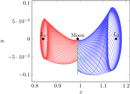
Figure 18. On the left: the propagation of manifolds from Halo around $L_{1}$ and Halo around $L_{2}$. On the right: the two trajectories of these manifold minimizing the distance on the plane $U_{2}$.

5.2.3. Three Short Transfers

Following our method, we compute three short transfers in order to initialize a multiple indirect shooting method and get the optimal trajectory.

From $\text{Halo}_{1}$ to $A_{\mathcal{M}_{1}}$.  Once again, we follow the method described in section 4.2.1, we construct two fixed points, one on $\text{Halo}_{1}$, the other on $A_{\mathcal{M}_{1}}$. To do that, we consider the two closest points on $\text{Halo}_{1}$ and $A_{\mathcal{M}_{1}}$. We choose two time parameters: $t_{\text{Halo}_{1}}$ to propagate backward the point on $\text{Halo}_{1}$ and $t_{A_{\mathcal{M}_{1}}}^{L_{1}}$ to propagate forward on $A_{\mathcal{M}_{1}}$. Here, we pick: $t_{\text{Halo}_{1}}=t_{A_{\mathcal{M}_{1}}}^{L_{1}}=$1.0$$. We are now ready to build the first optimal control problem as defined in (8). Using continuation on the final state solves this problem in an easy and fast ($4.1\text{\,}\mathrm{s}$) manner. The norm of the control is plotted in figure 19. Let us denote by $t_{0}=t_{\text{Halo}_{1}}+t_{A_{\mathcal{M}_{1}}}^{L_{1}}$, the transfer time and by $X_{0}^{*}=(\chi_{0}^{*},m_{0}^{*})$ and $X_{1}=(\chi_{1},m_{1})$ the terminal points of this transfer. The resulting final mass is $m_{1}=$1499.996\,743\,927\,8\text{\,}\mathrm{k}\mathrm{g}$$.

From $A_{\mathcal{M}_{1}}$ to $A_{\mathcal{M}_{2}}$.  In this part, we apply our method to compute the transfer from trajectory $A_{\mathcal{M}_{1}}$ to trajectory $A_{\mathcal{M}_{2}}$. There is a rather large gap to resorb. We already have the two points that we will perturb backward and forward: $\chi_{\mathcal{M}_{1}}^{U_{2}}$ and $\chi_{\mathcal{M}_{2}}^{U_{2}}$. We choose the two corresponding times $t_{\mathcal{M}_{1}}^{U_{2}}=t_{\mathcal{M}_{2}}^{U_{2}}=$0.5$$, and define the transfer time as $t_{2}=t_{\mathcal{M}_{1}}^{U_{2}}+t_{\mathcal{M}_{2}}^{U_{2}}$. After the first transfer from $\text{Halo}_{1}$ to $A_{\mathcal{M}_{1}}$, we follow a free trajectory on the manifold, so we choose the initial mass of the transfer from $A_{\mathcal{M}_{1}}$ to $A_{\mathcal{M}_{2}}$ as the final mass of the previous part, that is to say $m_{2}=m_{1}=$1499.996\,743\,927\,8\text{\,}\mathrm{k}\mathrm{g}$$.

Once again, the continuation on the final state allows for a fast convergence to obtain the solution of this problem. Indeed we obtained the solution in $4.4\text{\,}\mathrm{s}$. In this problem, we denote by $X_{2}=(\chi_{2},m_{2})$ the initial point on $A_{\mathcal{M}_{1}}$ and by $X_{3}=(\chi_{3},m_{3})$ the final point on $A_{\mathcal{M}_{2}}$. The final mass we get is $m_{3}=$1493.318\,462\,201\,5\text{\,}\mathrm{k}\mathrm{g}$$ and the norm of the control is plotted in figure 19.

From $A_{\mathcal{M}_{2}}$ to $\text{Halo}_{2}$.  We consider in here the last short transfer from $A_{\mathcal{M}_{2}}$ to $\text{Halo}_{2}$. Like the transfer from $\text{Halo}_{1}$ to $A_{\mathcal{M}_{1}}$, we pick the two closest points on $A_{\mathcal{M}_{2}}$ and $\text{Halo}_{2}$ and we perturb them with two time parameters denoted by $t_{\mathcal{M}_{2}}^{L_{2}}$ and $t_{\text{Halo}_{2}}$. We define then the transfer time $t_{4}=t_{\mathcal{M}_{2}}^{L_{2}}+t_{\text{Halo}_{2}}=(1.0+1.0)$ to go from $X_{4}=(\chi_{4},m_{4})$ to the final points $\chi_{5}^{*}$. As before, $m_{4}=m_{3}=$1493.318\,462\,201\,5\text{\,}\mathrm{k}\mathrm{g}$$ because after the transfer around $U_{2}$, we follow a free trajectory on the stable manifold.

Once again, the resolution is easy and fast thanks to the continuation method: $4.14\text{\,}\mathrm{s}$. The final mass we obtain is $m_{5}=$1493.315\,673\,696\,6\text{\,}\mathrm{k}\mathrm{g}$$. The norm of the control is plotted in figure 19.

Figure 19. Norm of the control for the three controlled parts of the admissible trajectory.

Admissible Trajectory in Five Parts.  To summarize, we have constructed an admissible trajectory going from $\text{Halo}_{1}$ to $\text{Halo}_{2}$ with three controlled parts and two free parts. This trajectory is plotted in the figure 20 and the control for the three controlled parts is in figure 19. The local transfers are computed with a maximal thrust equal to $180\text{\,}\mathrm{N}$, indeed this helps the convergence of local transfers (but we do not reach the targeted maximal thrust of $0.3\text{\,}\mathrm{N}$), and the multiple shooting for the reason described in section 4.2.1.

Figure 20. Admissible trajectory in five parts. Dashed part are manifold trajectories, i.e. free parts.

5.2.4. Multiple Shooting for the Total Transfer

We consider here the following problem

$$\mathcal{P}_{\text{tot}}^{\text{Halo}}\left\{\begin{array}[]{l}\displaystyle\mathcal{C}_{\text{tot}}=\min\int_{0}^{t_{\text{tot}}}\left\|u\right\|^{2}\mathrm{d}t,\\ \displaystyle\dot{x}=F_{0}(x)+\frac{\epsilon}{m}\sum_{i=1}^{3}u_{i}F_{i}(x),\\ \displaystyle\dot{m}=-\beta_{*}\epsilon\left\|u\right\|,\\ \left\|u\right\|\leqslant 1,\\ x(0)=\chi_{0}^{*}\in\text{Halo}_{1},\;m(0)=m_{0}^{*},\\[3.0pt] x(t_{\text{tot}})=\chi_{5}^{*}\in\text{Halo}_{2}.\end{array}\right.$$ (15)

Transfer time $t_{\text{tot}}$ is defined as $t_{\text{tot}}=t_{0}+t_{1}+t_{2}+t_{3}+t_{4},$ where $t_{0}$, $t_{2}$ and $t_{4}$ are the times previously introduced for the three short transfers. Time $t_{1}$ is the duration of trajectory $A_{\mathcal{M}_{1}}$ in the unstable manifold from $\text{Halo}_{1}$ from which we remove the two times we used to perturb points for the local transfers around $L_{1}$ and $U_{2}$. This gives us $t_{1}=t_{\mathcal{M}_{1}}-t_{A_{\mathcal{M}_{1}}}^{L_{1}}-t_{\mathcal{M}_{1}}^{U_{2}}$. And we defined $t_{3}$ in a similar way as $t_{3}=t_{\mathcal{M}_{2}}-t_{A_{\mathcal{M}_{2}}}^{L_{2}}-t_{\mathcal{M}_{2}}^{U_{2}}$. As in section 4.3, we introduced the shooting function with four nodes (for the Lyapunov to Lyapunov mission, we had two nodes). Because, we are considering a spatial mission, we get the following shooting function

$$\mathcal{S}_{\text{multi}}^{\text{Halo}}(Z)=\begin{pmatrix}\phi^{\text{ext}}_{1,\dots,7}(\chi_{0}^{*},m_{0}^{*},P_{0})-X_{1}\\ \phi^{\text{ext}}_{8,\dots,14}(\chi_{0}^{*},m_{0}^{*},P_{0})-P_{1}\\ \phi^{\text{ext}}_{1,\dots,7}(X_{1},P_{1})-X_{2}\\ \phi^{\text{ext}}_{8,\dots,14}(X_{1},P_{1})-P_{2}\\ \phi^{\text{ext}}_{1,\dots,7}(X_{2},P_{2})-X_{3}\\ \phi^{\text{ext}}_{8,\dots,14}(X_{2},P_{2})-P_{3}\\ \phi^{\text{ext}}_{1,\dots,7}(X_{3},P_{3})-X_{4}\\ \phi^{\text{ext}}_{8,\dots,14}(X_{3},P_{3})-P_{4}\\ \phi^{\text{ext}}_{1,\dots,6}(X_{4},P_{4})-\chi_{5}^{*}\\ \phi^{\text{ext}}_{14}(X_{4},P_{4})\\ \end{pmatrix}\in\mathbb{R}^{4\times 14+7},$$ (16)

where the vector $Z$ is defined as

$$Z=(\underbrace{p_{0},p_{m}^{0}}_{P_{0}},\underbrace{\chi_{1},m_{1}}_{X_{1}},\underbrace{p_{1},p_{m}^{1}}_{P_{1}},\underbrace{\chi_{2},m_{2}}_{X_{2}},\underbrace{p_{2},p_{m}^{2}}_{P_{2}},\underbrace{\chi_{3},m_{3}}_{X_{3}},\underbrace{p_{3},p_{m}^{3}}_{P_{3}},\underbrace{\chi_{4},m_{4}}_{X_{4}},\underbrace{p_{4},p_{m}^{4}}_{P_{4}})\in\mathbb{R}^{63}.$$

We initialize the shooting method with the values that we get from the local transfers and with a zero adjoint vector for the free parts. The shooting converges easily.

As for the two previous missions, we decrease the maximal authorized thrust by continuation. We then optimize the terminal points $\chi_{0}^{*}$ and $\chi_{5}^{*}$ to satisfy the transversality conditions. We manage to get the result in $4.16\text{\,}\mathrm{m}\mathrm{i}\mathrm{n}$. The final trajectory is plotted in figure 21 and the corresponding control in figure 22. The result cost is summarized in table 5 as well as the numerical values of the parameters. Because we are not comparing this mission with other published results, we just write the physical cost $\mathcal{C}_{\text{tot}}^{3}$ in the international system of units (see (14)). Note that we do not get the turnpike properties, indeed, in this case, there is no “steady-state” trajectory asymptotically connecting the two periodic orbits.

Initial Mass	Transfer time	$T_{\text{max}}$
$1500\text{\,}\mathrm{k}\mathrm{g}$	$9.543\,645\,446\,282\,8$ or $41.50\text{\,}\mathrm{d}\mathrm{a}\mathrm{y}\mathrm{s}$	$0.3\text{\,}\mathrm{N}$

	$\mathcal{C}_{\text{tot}}^{3}$	Mass of fuel
Halo to Halo Problem	$0.004\,619\,126\,477\,355\,13$	$7.415\,872\,590\,999\,92\text{\,}\mathrm{k}\mathrm{g}$

Table 5. Numerical results for the final trajectory of the Halo to Halo Mission.

Figure 21. Optimal trajectory for the Halo to Halo transfer. On the left, a 3 dimensional view. On the right, a view in the $(x,y)$-plane. The control is represented by arrows.

Figure 22. Optimal control for the Halo to Halo Mission $T(\cdot)\in\mathbb{R}^{3}$ in Newton.

6. Conclusion

To design different spacecraft missions between periodic orbits around Lagrange points, we have used natural (uncontrolled) trajectories computed thanks to the invariant manifolds of the periodic orbits. We have connected resulting arcs with short transfers using the PMP and indirect methods. Doing that, we have designed admissible trajectories performing the mission with controlled and uncontrolled parts. The resulting admissible trajectories have been used to initialize an indirect multiple shooting method in which we released the constraints to join uncontrolled parts, i.e., to force the spacecraft to follow the natural drift. We have finally obtained a trajectory satisfying the first order necessary conditions for optimality given by the PMP.

In order to improve the robustness of our indirect approach, we have designed and implemented appropriate continuations on the final state and on the thrust. Thanks to this, the execution of the overall computation is run within short time (of order of a few minutes), and results have the excellent accuracy of the underlying Newton method.

One can note that, when there is an heteroclinic orbit between the two terminal periodic orbits, the optimal enjoys a turnpike property. Proving the turnpike feature for such control-affine systems with drift is an open issue, which may deserve consideration because it gives an approach to successfully initialize a variant of the shooting method in a simple and efficient way (see [38]). Finally, as already mentioned, we have considered the $L^{2}$-minimization of the cost, leaving the computation of the $L^{1}$-minimization solution with a bang-bang control as an open issue for farther studies.

References

- [1] E. L. Allgower and K. Georg. Introduction to numerical continuation methods, volume 45 of Classics in Applied Mathematics. Society for Industrial and Applied Mathematics (SIAM), Philadelphia, PA, 2003. Reprint of the 1990 edition [Springer-Verlag, Berlin; MR1059455 (92a:65165)].
- [2] G. Archambeau, P. Augros, and E. Trélat. Eight-shaped Lissajous orbits in the Earth-Moon system. MathS in Action, 4(1):1–23, 2011.
- [3] R. Bertrand and R. Epenoy. New smoothing techniques for solving bang–bang optimal control problems—numerical results and statistical interpretation. Optimal Control Applications and Methods, 23(4):171–197, 2002.
- [4] B. Bonnard, L. Faubourg, and E. Trélat. Mécanique céleste et contrôle des véhicules spatiaux, volume 51 of Mathématiques & Applications (Berlin) [Mathematics & Applications]. Springer-Verlag, Berlin, 2006.
- [5] J.-B. Caillau. Contribution à l’étude du contrôle en temps minimal des transferts orbitaux. Thèse de doctorat, Institut National Polytechnique de Toulouse, Toulouse, France, novembre 2000.
- [6] J.-B. Caillau and B. Daoud. Minimum time control of the restricted three-body problem. SIAM J. Control Optim., 50(6):3178–3202, 2012.
- [7] Z. Chen, J.-B. Caillau, and Y. Chitour. -minimization for mechanical systems.
- [8] O. Cots, J.-B. Caillau, and J. Gergaud. Differential pathfollowing for regular optimal control problems. Optim. Methods Software, 27(2):177–196, 2012.
- [9] B. Daoud. Contribution au contrôle optimal du problème circulaire restreint des trois corps. Thèse de doctorat, Université de Bourgogne, novembre 2011.
- [10] R. Epenoy. Optimal long-duration low-thrust transfers between libration point orbits. In Proceedings of the 63rd International Astronautical Congress, volume 7, page 5670, Naples, Italy, 2012.
- [11] L. Euler. De motu rectilineo trium corpörum se mutuo attrahentium. Oeuvres, Seria Secunda tome XXv Commentationes Astronomicae:144–151, 1767.
- [12] R. W. Farquhar and A. A. Kamel. Quasi-periodic orbits about the translunar libration point. Celestial mechanics, 7(4):458–473, 1973.
- [13] R. W. Farquhar, D. P. Muhonen, C. R. Newman, and H. S. Heubergerg. Trajectories and Orbital Maneuvers for the First Libration-Point Satellite. Journal of Guidance, Control, and Dynamics, 3(6):549–554, 1980.
- [14] J. Gergaud and T. Haberkorn. Homotopy method for minimum consumption orbit transfer problem. ESAIM Control Optim. Calc. Var., 12(2):294–310 (electronic), 2006.
- [15] G. Gomez and J. Masdemont. Some zero cost transfers between libration point orbits. In Point Orbits, AAS paper 00-177, AAS/AIAA Astrodynamics Specialist Conference, 2000.
- [16] G. Gómez, J. Masdemont, and C. Simó. Lissajous orbits around halo orbits. Adv. Astronaut. Sci., 1997.
- [17] G. Gómez, J. Masdemont, C. Simó, and A. Jorba. Study refinement of semi-analytical halo orbit theory: Executive summary. ESOC Contract No.: 8625/89/D/MD (SC), 1991.
- [18] T. Haberkorn, P. Martinon, and J. Gergaud. Low thrust minimum-fuel orbital transfer: a homotopic approach. Journal of Guidance, Control, and Dynamics, 27(6):1046–1060, 2004. doi: 10.2514/1.4022.
- [19] F. Jiang, H. Baoyin, and J. Li. Practical techniques for low-thrust trajectory optimization with homotopic approach. Journal of Guidance, Control, and Dynamics, 35(1):245–258, 2012. doi: 10.2514/1.52476.
- [20] À. Jorba and J. Masdemont. Dynamics in the center manifold of the collinear points of the restricted three body problem. Phys. D, 132(1-2):189–213, 1999.
- [21] W. S. Koon, M. W. Lo, J. E. Marsden, and S. D. Ross. Dynamical systems, the three-body problem and space mission design. In International Conference on Differential Equations, Vol. 1, 2 (Berlin, 1999), pages 1167–1181. World Sci. Publ., River Edge, NJ, 2000.
- [22] W. S. Koon, M. W. Lo, J. E. Marsden, and S. D. Ross. Heteroclinic connections between periodic orbits and resonance transitions in celestial mechanics. Chaos, 10(2):427–469, 2000.
- [23] J.-L. Lagrange. Essai sur le problème des trois corps. Prix de l’académie royale des Sciences de paris, tome IX, Oeuvres de Lagrange 6, Gauthier-Villars:272–282, 1772.
- [24] C. Martin and B. A. Conway. Optimal low-thrust trajectories using stable manifolds. In Bruce A. Conway, editor, Spacecraft Trajectory Optimization, page 238–262. Cambridge University Press, 2010. Cambridge Books Online.
- [25] K. R. Meyer, G. R. Hall, and D. Offin. Introduction to Hamiltonian dynamical systems and the -body problem, volume 90 of Applied Mathematical Sciences. Springer, New York, second edition, 2009.
- [26] G. Mingotti, F. Topputo, and F. Bernelli-Zazzera. Combined optimal low-thrust and stable-manifold trajectories to the Earth-Moon halo orbits. AIP Conference Proceedings, 886(1):100–112, 2007.
- [27] G. Mingotti, F. Topputo, and F. Bernelli-Zazzera. Low-energy, low-thrust transfers to the Moon. Celestial Mechanics and Dynamical Astronomy, 105(1-3):61–74, 2009.
- [28] G. Mingotti, F. Topputo, and F. Bernelli-Zazzera. Optimal low-thrust invariant manifold trajectories via attainable sets. Journal of guidance, control, and dynamics, 34:1644–1655, 2011.
- [29] M. T. Ozimek and K. C. Howell. Low-thrust transfers in the Earth-Moon system, including applications to libration point orbits. Journal of Guidance, Control, and Dynamics, 33(2):533–549, 2010. doi: 10.2514/1.43179.
- [30] L. S. Pontryagin, V. G. Boltyanskii, R. V. Gamkrelidze, and E. F. Mishchenko. The mathematical theory of optimal processes. Translated by D. E. Brown. A Pergamon Press Book. The Macmillan Co., New York, 1964.
- [31] D. L. Richardson. Analytic construction of periodic orbits about the collinear points. Celestial Mech., 22(3):241–253, 1980.
- [32] J. Senent, C. Ocampo, and A. Capella. Low-thrust variable-specific-impulse transfers and guidance to unstable periodic orbits. Journal of Guidance, Control, and Dynamics, 28(2):280–290, 2005. doi: 10.2514/1.6398.
- [33] T. Starchville and R. Melton. Optimal low-thrust trajectories to Earth-Moon L2 Halo orbits (circular problem). In Proceedings of the AAS/AIAA Astrodynamics Specialists Conference, editor, Proceedings of the AAS/AIAA Astrodynamics Specialists Conference, pages 97–714. American Astro- nomical Soc., 1997.
- [34] Victor G. Szebehely. Theory of Orbits - The restricted problem of three bodies. Academic Press, 1967.
- [35] F. Topputo. Fast numerical approximation of invariant manifolds in the circular restricted three-body problem. Communications in Nonlinear Science and Numerical Simulation, 32:89 – 98, 2016.
- [36] E. Trélat. Contrôle optimal. Mathématiques Concrètes. [Concrete Mathematics]. Vuibert, Paris, 2005. Théorie & applications. [Theory and applications].
- [37] E. Trélat. Optimal control and applications to aerospace: some results and challenges. J. Optim. Theory Appl., 154(3):713–758, 2012.
- [38] E. Trélat and E. Zuazua. The turnpike property in finite-dimensional nonlinear optimal control. J. Differential Equations, 258(1):81–114, 2015.
- [39] L.T. Watson. HOMPACK90: FORTRAN 90 Codes for Globally Convergent Homotopy Algorithms. Department of Computer Science, Virginia Polytechnic Institute and State University, 1996.
- [40] F. B. Zazzera, F. Topputo, and M. Massari. Assessment of mission design including utilisation of libration points and weak stability boundaries. Technical Report 03-4103b, European Space Agency, the Advanced Concepts Team, 2004. Available on line at www.esa.int/act.
- [41] C. Zhang, F. Topputo, F. Bernelli-Zazzera, and Y.-S. Zhao. Low-thrust minimum-fuel optimization in the circular restricted three-body problem. Journal of Guidance, Control, and Dynamics, 38(8):1501–1510, 2015. doi: 10.2514/1.G001080.