Discrepancies between observational data and theoretical forecast in single field slow roll inflation

Abstract

The PLANCK collaboration has determined, or greatly constrained, values for the spectral parameters of the CMB radiation, namely the spectral index $n_{s}$, its running $\alpha_{s}$, the running of the running $\beta_{s}$, using a growing body of measurements of CMB anisotropies by the Planck satellite and other missions. These values do not follow the hierarchy of sizes predicted by single field, slow roll inflationary theory, and are thus difficult to fit for such inflation models.

In this work we present first a study of 49 single field, slow roll inflationary potentials in which we assess the likelyhood of these models fitting the spectral parameters to their currently most accurate determination given by the PLANCK collaboration. We check numerically with a MATLAB program the spectral parameters that each model can yield for a very broad, comprehensive list of possible parameter and field values. The comparison of spectral parameter values supported by the models with their determinations by the PLANCK collaboration leads to the conclusion that the data provided by PLANCK2015 TT+lowP and PLANCK2015 TT,TE,EE+lowP taking into account the running of the running disfavours 40 of the 49 models with confidence level at least 92.8%.

Next, we discuss the reliability of the current computations of these spectral parameters. We identify a bias in the method of determination of the spectral parameters by least residue parameter fitting (using MCMC or any other scheme) currently used to reconstruct the power spectrum of scalar perturbations. This bias can explain the observed contradiction between theory and observations. Its removal is computationally costly, but necessary in order to compare the forecasts of single field, slow roll theories with observations.

^aDepartament de Matemàtica Aplicada I, Universitat Politècnica de Catalunya
Diagonal 647, 08028 Barcelona, Spain

1 Introduction

Recent astronomical projects, notably the ongoing Planck collaboration, are mapping with ever greater detail the anisotropies of the CMB radiation, and determining the spectral parameters on which this radiation depends with increasing accuracy. Such a trove of data allows the submission of cosmological models to the test of comparing their forecasts with the observations.

The aim of this work is such a comparison. It concerns on one hand the power spectrum of the curvature fluctuation in comoving coordinates of the CMB

$${\mathcal{P}}_{\mathcal{R}}(k)=A_{s}\left(\frac{k}{k_{*}}\right)^{n_{s}-1+\frac{1}{2}\alpha_{s}\ln(\frac{k}{k_{*}})+\frac{1}{6}\beta_{s}\ln^{2}(\frac{k}{k_{*}})+\dots},$$

which governs the better discerned parts of the CMB and has been greatly constrained by the Planck collaboration (Ade et al. 2013, 2015), and on the other hand a family of 49 of the best known single field, slow roll inflationary models as compiled and systematized in (Martin, Ringeval & Vennin 2013) (see its Table 1).

Every one of the discussed slow roll inflation models admits a range of possible values for the slow roll parameters. Through the formulas recalled in Section 2, these parameters determine the successive coefficients of the Taylor series expansion of $\text{ln}\,{\mathcal{P}}_{\mathcal{R}}(k)$ at the chosen pivot scale $k_{*}$: the spectral index $n_{s}$, its running $\alpha_{s}$, the running of the running $\beta_{s}$, …

These spectral parameters $n_{s},\alpha_{s},\beta_{s}$ follow an approximately Gaussian distribution, and the Planck collaboration has produced determinations of their expected values and deviations. Therefore, it is a straightforward question for each single field, slow roll model to find out the possible range of values that it supports for these parameters, and check at what distance they lie from their values as determined by Planck.

The goal of our study is conceptually and practically simpler: to subject each model individually to the comparison between its forecast of spectral parameter values and the values actually found by (Ade et al. 2013, 2015), which give the most precise determination up to date. On the other hand, let us remark that is not the aim of this work to perform a Bayesian comparison between the models, as in (Martin, Ringeval & Trotta 2014), or to apply a Bayesian test of relevance to the spectral parameters as in (Giannantonio & Komatsu 2015).

The interest of such a simple analysis of model forecasts vs observations can be inferred from the values that (Ade et al. 2013, 2015) atribute to the running $\alpha_{s}$ and running of the running $\beta_{s}$. According to single field, slow roll inflation $n_{s}-1$ is of order 1, $\alpha_{s}$ of order 2, and $\beta_{s}$ of order 3 in the inflation parameters $\epsilon,\eta$ (see Sect. 2). Yet in all the determinations of the Planck team the running $\alpha_{s}$, or the running of the running $\beta_{s}$ have the same order of magnitude as $n_{s}-1$, namely $10^{-2}$. This is a hint of a strong disagreement between theoretical forecasts and observations.

The causes for this discordance of orders of magnitude may lie in the lack of precission either of the theoretical models or of the observed, actually computed from CMB measurements, values for the spectral parameters. This is the topic discussed in Section 4, where it is found that there is a subtle mathematical cause of inaccuracy in the computation of the values of the spectral parameters in the highest-likelyhood fits currently used.

This is not a problem with the employed statistical techniques, but with the mathematical meaning of the spectral parameters: they are the coefficients of the Taylor expansion of the function $\ln{\mathcal{P}}_{\mathcal{R}}(k)$ at a pivot scale $k_{*}$, thus they yield the best possible approximation of this function with a polynomial of a specified degree in a suitably small neighbourhood of $k_{*}$. In contrast, any likelyhood-maximizing method seeks the polynomial of the specified degree that best approximates $\ln{\mathcal{P}}_{\mathcal{R}}(k)$ in a fixed interval $[k_{*},k_{final}]$. The regression polynomial of a specified degree for a function $g(k)$ in a fixed interval $[k_{*},k_{final}]$, and the likelyhood-maximizing polynomials that can be characterized as regression polynomials with a suitable weighted inner product, are different from the Taylor polynomial of $g(k)$ at the point $k_{*}$. In Sect. 4 we show, both with an elementary example using linear least square fitting and with an actual computation of spectral parameters by residue minimization, how the order of magnitude discrepancy between the coefficients of the two polynomials often mimics closely that between Planck’s evaluations and the theoretical determinations of the running $\alpha_{s}$ and the running of the running $\beta_{s}$. While this interpretation flaw does not affect a Bayesian discussion of whether higher order terms in $\ln{\mathcal{P}}_{\mathcal{R}}(k)$ are necessary for the description of the CMB power spectrum, it has to be solved in order to obtain a meaningful comparison between theoretical models and observations.

The units used in the paper are: $\hbar=c=8\pi G=1.$

2 Slow-roll parameters

In slow roll inflation (see Basset, Tsujikawa & Wands (2006) for a review of inflation) the commonly used first order parameters are:

$$\epsilon=-\frac{\dot{H}}{H^{2}}\cong\frac{1}{2}\left(\frac{V_{\varphi}}{V}\right)^{2}\quad\mbox{and}\quad\eta=2\epsilon-\frac{\dot{\epsilon}}{2H\epsilon}\cong\frac{V_{\varphi\varphi}}{V}.$$ (1)

At the first slow roll order, the spectral index of scalar perturbations and its running are given by

$${n}_{s}-1=2\eta-6\epsilon\quad\mbox{and}\quad{\alpha}_{s}=16\epsilon\eta-24\epsilon^{2}-2\xi,$$ (2)

where the second order slow roll parameter

$$\xi\equiv\left(2\epsilon-\frac{\dot{\eta}}{{H}\eta}\right)\eta\cong\frac{V_{\varphi}V_{\varphi\varphi\varphi}}{V^{2}},$$ (3)

has been introduced.

Moreover, in inflationary cosmology, the tensor/scalar ratio, namely $r$, is related with the slow roll parameter $\epsilon$, via the following consistency relation ${r}=16\epsilon.$

The other important parameter that we will use in this work is the running of the running $\beta_{s}=\frac{d\alpha_{s}}{d\ln k}$, given, in the slow roll approximation, by (Huang 2006; Ade et al. 2013)

$$\beta_{s}=-192{\epsilon}^{3}+192{\epsilon}^{2}\eta-32\epsilon{\eta}^{2}-24\epsilon\xi+2\eta\xi+2\zeta,$$ (4)

where we have introduced the third order slow roll parameter

$$\zeta\equiv\left(4\epsilon-\eta-\frac{\dot{\xi}}{H\xi}\right)\xi\cong\frac{V^{2}_{\varphi}V_{\varphi\varphi\varphi\varphi}}{V^{3}}.$$ (5)

3 PLANCK2015 data: the running of the running

The last PLANCK2015 data about the running $\alpha_{s}$ and its running $\beta_{s}=\frac{d\alpha_{s}}{d\ln k}$ are reproduced in Table 1.

Determination	$n_{s}$	$\alpha_{s}$	$\beta_{s}$
PLANCK2015 TT+lowP	$0.9569\pm 0.0077$	$0.011^{+0.014}_{-0.013}$	$0.029^{+0.015}_{-0.016}$
PLANCK2015 TT,TE,EE+lowP	$0.9586\pm 0.0056$	$0.009\pm 0.010$	$0.025\pm 0.013$

Table 1: Determinations, or constrains in case of being nontrivial, of the spectral parameter values, with running of the running by PLANCK2015 ((19) of Ade et al. (2015))

These results contradict single field slow roll inflation, because in that case, the running $\alpha_{s}$ is second order in the slow roll parameters, and its running is given by Eqs. (4), (5), which make $\beta_{s}$ a third order parameter, while the values determined by PLANCK place $\beta_{s}$ in a higher order of magnitude than the running $\alpha_{s}$ itself. Moreover, disregarding the running of the running, the running is negative while taking into account it, the running becomes positive. This seems a signature of the problem that suffers the method used to reconstruct the power spectrum of scalar perturbations from observational data: the value of the coefficients in the Taylor series of the power spectrum logarithm function could suffer a bias. We will address this question later.

To show the improbability of the observed value of $\beta_{s}$ analytically for all the potentials that appear in (Martin, Ringeval & Vennin 2013) is very involved due to the increasing complexity of the formulas (4), (5) for the new parameter $\beta_{s}$. However in the case of LI (with $\alpha>0$), SFI and BI (with $p$ and even number), HTI, ESI, PLI and LFI, a simple calculation shows that $\beta_{s}\leq 0$ which means that the deviation from the theoretical value of the running of the running to its expected observational value is larger than $1.9\sigma$, using both, PLANCK2015 TT,TE,EE+lowP or PLANCK2015 TT+lowP data.

The other potentials appearing in (Martin, Ringeval & Vennin 2013) are analysed numerically.

3.1 Numerical fitting of the parameters

Let us describe the numerical tests that the authors have applied to all single field inflationary models from the list of (Martin, Ringeval & Vennin 2013). These tests have been built into a MATLAB program that takes as input a list of potentials $V(\varphi)$ and values for spectral parameters in the list $r,n_{s},\alpha_{s},\beta_{s}$, and asseses the likelihood of each model in the list to fit the values of the running of the running $\beta_{s}$, assuming Gaussian distribution for all the spectral parameters.

For each cosmological model, a broad range of possible values for the parameters on which it depends has been determined following (Martin, Ringeval & Vennin 2013). A test list of values for each parameter has been selected, covering in a dense, equispaced fashion finite intervals of possible values for the parameter, and approaching with log-equispaced values every finite or infinite limit value for the parameter.

The MATLAB software developed by the authors, for each model $V(\varphi)$ and choice of value of the parameter(s) on which it depends, takes an equispaced mesh of values in the range $[\varphi_{0},\varphi_{f}]$ of possible values of the field in this model. This mesh is taken increasingly fine, currently up to step $\Delta\varphi=2\cdot 10^{-4}$.

The subintervals in the range of field values for which the potential satisfies $V(\varphi)>0$ are numerically determined over the selected mesh, and each interval of positive values of the potential for the selected values of the model parameters is considered as a case, which thus consists of:

• a candidate theory with a given potential $V(\varphi)$,

• a specific choice of parameter values for $V(\varphi)$,

• and a range of values $[\bar{\varphi}_{0},\bar{\varphi}_{f}]$ of the inflaton field $\varphi$ such that $V(\varphi)>0$ on them.

The numerical test for each case consists in meshing the interval of field values with a uniform step (of size $\Delta\varphi=2\cdot 10^{-4}$ for the results reported in this work), computing the spectral parameters $r,n_{s},\alpha_{s},\beta_{s}$ for each value of the field $\varphi$ in the mesh using the formulas of Section 2 and symbolic derivation of the potential $V$ to produce the derivatives $V_{\varphi},\dots,V_{\varphi\varphi\varphi\varphi}$, and then applying successive filtering criteria to determine which values of the field $\varphi$ fulfill simultaneously all of them, thus allowing the model in this particular case to fit the spectral measured data for which the model is tested.

PLANCK2015 provides the main values of the spectral paramenters, namely $<n_{s}>,<\alpha_{s}>,<\beta_{s}>$, and their standard deviations of the respective one-dimensional marginalized posterior distribution, namely $\sigma_{n_{s}},\sigma_{\alpha_{s}},\sigma_{\beta_{s}}$.

The applied filters in the case of spectral parameters with running of the running consist in looking for the values of the field $\varphi$ such that:

1. $\epsilon(\varphi)\leq 1$, $|\eta(\varphi)|\leq 1$, $|\xi(\varphi)|\leq 1$ and $|\zeta(\varphi)|\leq 1$.

2. The number of e-folds $N(\varphi)$ ranges between $50$ and $60$.

3. $|\beta_{s}(\varphi)-<\beta_{s}>|<1.8\sigma_{\beta_{s}}$.

Then, dealing with the one-dimensional marginalized posterior distribution of the running of the running, a model not passing this filter is ruled out with 92.8 % C.L..

Remark 3.1.

The testing software looks for values of the field $\varphi_{e}$ such that $\epsilon(\varphi_{e})\cong 1$, and using them as endpoints of the inflationary phase, computes the number of e-folds of inflation for any choice of $\varphi$ in the case, by integrating numerically with a trapezoidal rule

$$N(\varphi)=\left|\int_{\varphi_{e}}^{\varphi}\frac{V}{V_{\varphi}}d\varphi\right|.$$ (6)

Finally, it is important to realize that in our analysis the one-dimensional marginalized 92.8 % C.L. interval for $\beta_{s}$ is compared to the theoretical predictions of inflationary models, and differs form the usual one where the marginalized joint 95.5 % C.L. region for ($n_{s}$, $r$) without a running spectral index is compared with the theoretical forecast.

3.2 Numerical results

Single-field inflaton models were exhaustively studied in (Martin, Ringeval & Vennin 2013), from which we take the list of models and parameters to be numerically tested. Table LABEL:t:llistamodels, adapted from Table 1 of (Martin, Ringeval & Vennin 2013), presents each model’s potential, the range of values of the parameters for which it has been tested, and the range of values of the inflaton field over which it has been tested.

Table 2: Models from (Martin, Ringeval & Vennin 2013) numerically tested. Parameter values expressed in Matlab code: linspace(a,b,n) means $n$ equispaced values between $a$ and $b$; 10.$\wedge$linspace(a,b,n) means $n$ log-equispaced values between $10^{a}$ and $10^{b}$. Parameter $V_{0}$ and the reduced Planck mass $M_{\text{Pl}}$ always set to 1. The range of studied field values is $\varphi\in[10^{-4},40]$ unless otherwise indicated.

Name	$V(\varphi)$	Parameter values	Field values
HI	$V_{0}\left(1-e^{-\sqrt{2/3}\varphi}\right)^{2}$		[-40,40]
RCHI	$V_{0}\left(1-2e^{-\sqrt{2/3}\varphi}+\frac{A_{I}}{16\pi^{2}}\frac{\varphi}{\sqrt{6}}\right)$	$A_{I}$: [linspace(-100,100,120),linspace(-3,3,200)]	[-10,20]
LFI	$V_{0}\left(\varphi\right)^{p}$	$p$: linspace(0.5,20,60)
MLFI	$V_{0}\varphi^{2}\left[1+\alpha\varphi^{2}\right]$	$\alpha$: [linspace(-10,100,61),linspace(-0.1,0.1,120)]
RCMI	$V_{0}\left(\varphi\right)^{2}\left[1-2\alpha\varphi^{2}\ln\left(\varphi\right)\right]$	$\alpha$: [linspace(1e-4,1.5,30),10.$\wedge$linspace(-14,-5,20)]
RCQI	$V_{0}\left(\varphi\right)^{4}\left[1-\alpha\ln\left(\varphi\right)\right]$	$\alpha$: [linspace(1e-2,10,120),10.$\wedge$linspace(-6,-2.5,10)]
NI	$V_{0}\left[1+\cos\left(\frac{\varphi}{f}\right)\right]$	$f$: 1	$[10^{-5},\pi]$
ESI	$V_{0}\left(1-e^{-q\varphi}\right)$	$q$: [linspace(0.1,10,120),linspace(1e-5,0.099,60)]
PLI	$V_{0}e^{-\alpha\varphi}$	$\alpha$: [linspace(0.1,10,120),10.$\wedge$linspace(-6,-1.5,15)]	[-40,40]
KMII	$V_{0}\left(1-\alpha\varphi e^{-\varphi}\right)$	$\alpha$: [linspace(1e-2,10,60),10.$\wedge$linspace(-6,-2.5,10)]
HF1I	$V_{0}\left(1+A_{1}\varphi\right)^{2}\left[1-\frac{2}{3}\left(\frac{A_{1}}{1+A_{1}\varphi}\right)^{2}\right]$	$A_{1}$: linspace(1e-3,40,180)	[-40,40]
CWI	$V_{0}\left[1+\alpha\left(\frac{\varphi}{Q}\right)^{4}\ln\left(\frac{\varphi}{Q}\right)\right]$	$Q$: [10.$\wedge$linspace(-6,-2.5,12),linspace(1e-2,10,60)]
LI	$V_{0}\left[1+\alpha\ln\left(\varphi\right)\right]$	$\alpha$: [linspace(-0.3,0.3,60),-10.$\wedge$linspace(-1,0,10),10.$\wedge$linspace(-1,0,10)]
RpI	$V_{0}e^{-2\sqrt{2/3}\varphi}\left|e^{\sqrt{2/3}\varphi}-1\right|^{2p/(2p-1)}$	$p$: linspace(0.25,10,60)
DWI	$V_{0}\left[\left(\frac{\varphi}{\varphi_{0}}\right)^{2}-1\right]^{2}$	$\varphi_{0}$: 1	$[10^{-4},80]$
MHI	$V_{0}\left[1-\text{sech}\left(\frac{\varphi}{\mu}\right)\right]$	$\mu$: 10	$[10^{-4},400]$
RGI	$V_{0}\frac{\left(\varphi\right)^{2}}{\alpha+\left(\varphi\right)^{2}}$	$\alpha$: [linspace(1e-1,10,30),10.$\wedge$linspace(-6,-1.5,12)]
MSSMI	$V_{0}\left[\left(\frac{\varphi}{\varphi_{0}}\right)^{2}-\frac{2}{3}\left(\frac{\varphi}{\varphi_{0}}\right)^{6}+\frac{1}{5}\left(\frac{\varphi}{\varphi_{0}}\right)^{10}\right]$	$\varphi_{0}$: [1e-7,1e-3,1]	$[10^{-4},80]$
RIPI	$V_{0}\left[\left(\frac{\varphi}{\varphi_{0}}\right)^{2}-\frac{4}{3}\left(\frac{\varphi}{\varphi_{0}}\right)^{3}+\frac{1}{2}\left(\frac{\varphi}{\varphi_{0}}\right)^{4}\right]$	$\varphi_{0}$: [1e-7,1e-3,1]	$[10^{-4},80]$
AI	$V_{0}\left[1-\frac{2}{\pi}\arctan\left(\frac{\varphi}{\mu}\right)\right]$	$\mu$: [1e-2,1]	[-40,40]
CNAI	$V_{0}\left[3-\left(3+\alpha^{2}\right)\tanh^{2}\left(\frac{\alpha}{\sqrt{2}}\varphi\right)\right]$	$\alpha$: [linspace(1e-2,20,120),10.$\wedge$linspace(-6,-2.5,10)]
CNBI	$V_{0}\left[\left(3-\alpha^{2}\right)\tan^{2}\left(\frac{\alpha}{\sqrt{2}}\varphi\right)-3\right]$	$\alpha$: [linspace(1e-3,5,40),10.$\wedge$linspace(-7,-3.5,12)]
OSTI	$-V_{0}\left(\frac{\varphi}{\varphi_{0}}\right)^{2}\ln\left[\left(\frac{\varphi}{\varphi_{0}}\right)^{2}\right]$	$\varphi_{0}$: 1	$[10^{-6},1]$
WRI	$V_{0}\ln^{2}\left(\frac{\varphi}{\varphi_{0}}\right)$	$\varphi_{0}$: 1	$[10^{-4},10]$
SFI	$V_{0}\left[1-\left(\frac{\varphi}{\mu}\right)^{p}\right]$	$\mu$: 1 $p$: linspace(0.5,10,20)	$[10^{-4},1]$
II	$V_{0}\left(\varphi-\varphi_{0}\right)^{-\beta}-V_{0}\frac{\beta^{2}}{6}\left(\varphi-\varphi_{0}\right)^{-\beta-2}$	$\varphi_{0}$: 0 $\beta$: [linspace(0.1,10,31),linspace(20,50,3)]
KMIII	$V_{0}\left[1-\alpha(\varphi)^{\frac{4}{3}}\exp\left(-\beta(\varphi)^{\frac{4}{3}}\right)\right]$	$\alpha$: 10.$\wedge$linspace(-3,12,46) $\beta$: 10.$\wedge$linspace(-3,12,46)	$[10^{-4},10]$
LMI	$V_{0}\left(\varphi\right)^{\alpha}\exp\left[-\beta(\varphi)^{\gamma}\right]$	$\beta$: [linspace(0.1,20,40),10.$\wedge$linspace(-4,-1.5,10)] $\gamma$: [linspace(1e-3,2,30),10.$\wedge$linspace(0.5,2,4),10.$\wedge$linspace(-6,-4,3)]
TWI	$V_{0}\left[1-A\left(\frac{\varphi}{\varphi_{0}}\right)^{2}e^{-\varphi/\varphi_{0}}\right]$	$\varphi_{0}$: 1 $A$: linspace(0.001,8,120)
GMSSMI	$V_{0}\left[\left(\frac{\varphi}{\varphi_{0}}\right)^{2}-\frac{2}{3}\alpha\left(\frac{\varphi}{\varphi_{0}}\right)^{6}+\frac{\alpha}{5}\left(\frac{\varphi}{\varphi_{0}}\right)^{10}\right]$	$\varphi_{0}$: 10.$\wedge$linspace(-2,0,3) $\alpha$: [linspace(1e-2,2.5,120),10.$\wedge$linspace(0.5,1.5,3),10.$\wedge$linspace(-4,-2.5,6)]
GRIPI	$V_{0}\left[\left(\frac{\varphi}{\varphi_{0}}\right)^{2}-\frac{4}{3}\alpha\left(\frac{\varphi}{\varphi_{0}}\right)^{3}+\frac{\alpha}{2}\left(\frac{\varphi}{\varphi_{0}}\right)^{4}\right]$	$\varphi_{0}$: 10.$\wedge$linspace(-2,0,3) $\alpha$: linspace(0.1,10,120)	$[10^{-4},20]$
BSUSYBI	$V_{0}\left(e^{\sqrt{6}\varphi}+e^{\sqrt{6}\gamma\varphi}\right)$	$\gamma$: linspace(1e-5,2,200)	[-40,40]
TI	$V_{0}\left(1+\cos\frac{\varphi}{\mu}+\alpha\sin^{2}\frac{\varphi}{\mu}\right)$	$\mu$: 1 $\alpha$: [linspace(0.01,3,80),10.$\wedge$linspace(-4,-2.5,6),10.$\wedge$linspace(1,2,4)]
BEI	$V_{0}\exp_{1-\beta}\left(-\lambda\varphi\right)$	$\beta$: [linspace(-5,5,60),10.$\wedge$linspace(1,2,3),10.$\wedge$linspace(-4,-2,3), -10.$\wedge$linspace(1,2,3),-10.$\wedge$linspace(-4,-2,3)] $\lambda$: 1	[-100,100]
PSNI	$V_{0}\left[1+\alpha\ln\left(\cos\frac{\varphi}{f}\right)\right]$	$\alpha$: [linspace(0.1,10,60),10.$\wedge$linspace(-4,-1.5,12)] $f$: 1	$[10^{-4},\pi/2-10^{-4}]$
NCKI	$V_{0}\left[1+\alpha\ln\left(\varphi\right)+\beta\left(\varphi\right)^{2}\right]$	$\alpha$: 10.$\wedge$linspace(-7,0,16) $\beta$: linspace(-10,10,80)
CSI	$\frac{V_{0}}{\left(1-\alpha\varphi\right)^{2}}$	$\alpha$: [linspace(0.1,5,100),10.$\wedge$linspace(-4,-1.5,8),10.$\wedge$linspace(1,2,4)]	[-40,40]
OI	$V_{0}\left(\frac{\varphi}{\varphi_{0}}\right)^{4}\left[\left(\ln\frac{\varphi}{\varphi_{0}}\right)^{2}-\alpha\right]$	$\varphi_{0}$: 1 $\alpha$: [10.$\wedge$linspace(-7,-2,18),linspace(0.03,1,40)]
CNCI	$V_{0}\left[\left(3+\alpha^{2}\right)\coth^{2}\left(\frac{\alpha}{\sqrt{2}}\varphi\right)-3\right]$	$\alpha$: [linspace(0.1,5,40),10.$\wedge$linspace(-7,-1.5,12),10.$\wedge$linspace(1,3,5)]
SBI	$V_{0}\left\{1+\left[-\alpha+\beta\ln\left(\varphi\right)\right]\left(\varphi\right)^{4}\right\}$	$\alpha$: 10.$\wedge$linspace(-8,0,27) $\beta$: 10.$\wedge$linspace(-8,0,27)
SSBI	$V_{0}\left[1+\alpha\left(\varphi\right)^{2}+\beta\left(\varphi\right)^{4}\right]$	$\alpha$: [-10.$\wedge$linspace(-5,2,24),10.$\wedge$linspace(-5,2,24)] $\beta$: [-10.$\wedge$linspace(-5,2,24),10.$\wedge$linspace(-5,2,24)]	$[10^{-4},20]$
IMI	$V_{0}\left(\varphi\right)^{-p}$	$p$: linspace(0.5,10,40)
BI	$V_{0}\left[1-\left(\frac{\varphi}{\mu}\right)^{-p}\right]$	$p$: [linspace(1,10,37),10.$\wedge$linspace(-1,-0.33,3)] $\mu$: [1e-4,1]
RMI	$V_{0}\left[1-\frac{c}{2}\left(-\frac{1}{2}+\ln\frac{\varphi}{\varphi_{0}}\right)\varphi^{2}\right]$	$\varphi_{0}$: 1 $c$: [-linspace(2,10,33),-10.$\wedge$linspace(-5,0,15),10.$\wedge$linspace(-5,0,14), linspace(2,10,33)]	$[10^{-4},10]$
VHI	$V_{0}\left[1+\left(\frac{\varphi}{\mu}\right)^{p}\right]$	$\mu$: 1 $p$: linspace(0.1,12,80)
DSI	$V_{0}\left[1+\left(\frac{\varphi}{\mu}\right)^{-p}\right]$	$\mu$: 1 $p$: linspace(0.1,12,80)
GMLFI	$V_{0}\left(\varphi\right)^{p}\left[1+\alpha\left(\varphi\right)^{q}\right]$	$\alpha$: 10.$\wedge$linspace(-7,3,31) $p$: linspace(0.5,12,24) $q$: linspace(0.5,12,24)	[-40,40]
LPI	$V_{0}\left(\frac{\varphi}{\varphi_{0}}\right)^{p}\left(\ln\frac{\varphi}{\varphi_{0}}\right)^{q}$	$\varphi_{0}$: 1 $p$: [linspace(0.5,12,24),10.$\wedge$linspace(1.5,2,2)] $q$: [linspace(0.5,12,24),10.$\wedge$linspace(1.5,2,2)]
CNDI	$\frac{V_{0}}{\left\{1+\beta\cos\left[\alpha\left(\varphi-\varphi_{0}\right)\right]\right\}^{2}}$	$\varphi_{0}$: 0 $\alpha$: [linspace(0.1,1,30),10.$\wedge$linspace(-3,-1.5,4),10.$\wedge$linspace(0.5,2,4)] $\beta$: [linspace(1,10,30),10.$\wedge$linspace(-2,-0.5,8),10.$\wedge$linspace(1.5,2,3), -10.$\wedge$linspace(-2,1,7)]

The models, choice of parameter values and range of field values of Table LABEL:t:llistamodels have been subjected to the numerical test described in subsection 3.1 for the several determinations of the spectral parameters $n_{s},\alpha_{s},\beta_{s}$. Let us sum up the conclusions:

For the determination of spectral parameters PLANCK2015 TT+lowP and PLANCK2015 TT,TE,EE+lowP with running of the running of Table 1, the only models in Table LABEL:t:llistamodels which are not disproved for any choice of parameter and field values with confidence at least 92.8% (the distance of the theoretical value of the runnig of the running to its mean observational data is larger than $1.8\sigma_{\beta}$) are:

1. Loop Infation (LI) (Binetruy & Dvali 1996; Halyo 1996)

2. $R+R^{2p}$ Inflation (RpI) (Tsujikawa & De Felice 2010; Nojiri & Odintsov 2011).

3. Kähler Moduli Inflation II (KMIII) (Colon & Quevedo 2006; Lee & Nam 2001)

4. Logamediate Inflation (LMI) (Parson & Barrow 1995; Barrow & Nunes 2007).

5. Brane SUSY Breaking Inflation (BSUSYBI) (Martin & Ringeval 2004 ; Dudas et al. 2012).

6. Spontaneous Symmetry Breaking Inflation (SSBI) (Albercht & Brandenberger 1985; Hu and O’Connor 1986).

7. Tip Inflation (TI) (Pajer 2008).

8. Generalised Mixed Large Field Inflation (GMLFI) (Kinney & Riotto 1998, 1999).

9. Constant $n_{s}$ D Inflation (CNDI) (Hodges & Blumenthal 1999).

(albeit LI is disproved with 95.5% confidence, when one deals with the one-dimensional marginalized posterior distribution of the spectral index $n_{s}$).

4 Accuracy and reliability of the spectral parameter values

The computation of the spectral parameters from a single field, slow roll theory with potential $V(\varphi)$, recalled in Sect. 2, forecasts that the spectral index $n_{s}-1$ has order 1 on the inflation parameters $\epsilon,\eta$, the running $\alpha_{s}$ has order 2 on $\epsilon,\eta$, i.e. $\alpha_{s}=O((n_{s}-1)^{2})$ because $\epsilon,\eta$ are small, and the running of the running $\beta_{s}$ has order 3, i.e. $\beta_{s}=O((n_{s}-1)^{3})$.

The successive evaluations of the spectral parameters in (Ade et al. 2013, 2015) do not support this forecast:

1. The Planck 2013 determination without running of the running, finds $|n_{s}-1|\approx 4\cdot 10^{-2}$, $\alpha_{s}\approx 2\cdot 10^{-2}$, the latter 2 standard deviations away from having a lower order.

2. The Planck 2015 determination without running of the running, finds again $|n_{s}-1|\approx 4\cdot 10^{-2}$, and now $\alpha_{s}\approx 10^{-2}$, with standard deviation $\sigma\approx 10^{-2}$, i.e. $\alpha_{s}$ is only $1\sigma$ away from having a lower order.

3. But the Planck 2015 determination with running of the running, finds $|n_{s}-1|\approx 4\cdot 10^{-2}$, $\alpha_{s}\approx 10^{-2}$ with deviation $\sigma\approx 10^{-2}$, and $\beta_{s}\approx 3\cdot 10^{-2}$, with the running of the running $2\sigma$ away from having a lower order.

Therefore, the value of our simple analysis comparing model forecasts and experimental determinations depends on the reliability of these determinations of the values of the spectral parameters.

The methodology for this determination used in (Ade et al. 2013, 2015) is based on model fitting through Bayesian statistical techniques and Markov-Monte Carlo (MCMC) optimization techniques. We have identified a flaw with the mathematical foundations of this procedure, which will lead to incorrect values of the spectral parameters.

This flaw comes from an inaccurate interpretation of the meaning of the Taylor expansion of a function, and is independent of the statistical and optimization techniques used to fit the values, manifesting itself with similar consequences in computations with procedures ranging from least square optimization to Bayesian likelihood maximization with MCMC methods. A very common manifestation of this flaw is the overestimation of the size of the highest order coefficient in the sought function.

We need to review the mathematical underpinnings of Taylor series expansions and the method for the estimation of the spectral parameters in order to explain the flaw.

The Taylor expansion of a function $g(\kappa)$ at a pivot scale $\kappa=0$ puts $g$ as a limit of a sequence of Taylor polynomials $S_{d}(g)=\sum_{i=0}^{d}\frac{g^{i)}(0)}{i!}\kappa^{i}$ with increasing degree $d$. These polynomials are determined by the successive derivatives of $g$ at 0, $g(0),g^{\prime}(0),\dots,g^{d)}(0)$, and have the property that $S_{d}(g)$ is the polynomial of a fixed maximal degree $d$ that best fits the values of the function $g(\kappa)$ for $\kappa$ in intervals $(-\delta,\delta)$ with $\delta<<1$. That is, the fit of the polynomial $S_{d}$ to the function $g$ is optimal in a very small neighbourhood of $\kappa=0$, and becomes worse, indeed irrelevant, for values of $\kappa$ outside this neighbourhood.

When we try to approximate a function $g(\kappa)$ with a polynomial $p(\kappa)$ by minimizing a residue vector defined by the integrals over some family of test functions $\{\varphi_{l}\}$,

$$R(p)=\left(\dots\int_{0}^{\kappa_{f}}\varphi_{l}(\kappa)p(\kappa)d\kappa-\int_{0}^{\kappa_{f}}\varphi_{l}(\kappa)g(\kappa)d\kappa\dots\right)$$

the fit of the values of the polynomial $p(\kappa)$ to the function $g(\kappa)$ is important all over the integration interval $[0,\kappa_{f}]$. If the test functions in the family $\{\varphi_{l}\}$ have its peaks and troughs well spread over the integration interval, the fit of the values of $p(\kappa)$ to the values of $g(\kappa)$ is of roughly equal importance in all of the interval $[0,\kappa_{f}]$.

This is the mathematical reason why the polynomial of a fixed degree $d$ best approximating a function $g(\kappa)$ through minimization of some residue defined over an interval $[0,\kappa_{f}]$ will not be the Taylor polynomial of degree $d$ of $g$ at the pivot scale $\kappa=0$.

A concrete and frequent manifestation of this problem is that if one tries to fit with a polynomial of a fixed degree $d$ the values of a function $g(\kappa)$, over a fixed interval $[0,\kappa_{f}]$ where $g$ has order of growth higher than $\kappa^{d}$, the residue–minimizing fit for any reasonable evaluation of the residue will produce a polynomial whose greatest degree coefficient is inflated in comparison to the corresponding Taylor series coefficient of $g$, in order for the leading term $a_{d}\kappa^{d}$ of the polynomial to approach a growth of $g$ that actually has higher order.

We can illustrate this phenomenon with an elementary example: the approximation of the function $g(\kappa)=\kappa^{4}$ by taking 100 equispaced values of $g$ in the interval $[0,3]$, and finding the polynomial $p_{d}$ of fixed degree $d$ that for the table of equispaced values $(\kappa_{i},g(\kappa_{i}))$ minimizes the residue $\sum_{i=1}^{100}\left(g(\kappa_{i})-p_{d}(\kappa_{i})\right)^{2}$. That is, $p_{d}$ is the classical least square fit polynomial of degree $d$ for the tabulated values of $g$. The results are summarized in Table 3.

degree $d$ of fit	$a_{0}$	$a_{1}$	$a_{2}$	$a_{3}$	$a_{4}$
$\geq 4$ (exact values)	0	0	0	0	1
3	-1.09	7.60	-11.53	6
2	6.77	-24.64	15.47
1	-16.20	21.76
0	16.45

Table 3: Regression polynomial and the overestimations for the leading coefficients.

As $g$ is a polynomial of degree 4, once the regression polynomial is allowed to reach this degree the least square polynomial $p_{d}$ is exactly $g$, and in particular the coefficients of $p_{d}$ are exactly the coefficients of the Taylor expansion of $g$ at $\kappa=0$. But when a polynomial $p_{d}=a_{0}+a_{1}\kappa+\dots+a_{d}\kappa^{d}$ of a degree $d<4$ is fit, the least square fit results in a systematic bias: the leading coefficient $a_{d}$ is greatly overestimated compared to the coefficient of the same degree in $g$, because the term $a_{d}\kappa^{d}$ follows values of $g$ with a growth rate greater than $d$. This overestimation of the leading coefficient results in a cascade of alternating over- and underestimations for the lower degree coefficients of the polynomial.

The same problem, further complicated by the fact that the sought function is not polynomial and thus has infinitely many nonvanishing Taylor expansion coefficients, happens with the estimation of the spectral parameters of the power spectrum through MCMC optimization (Ade et al. 2013, 2015): one starts with the multipolar expansion of the CMB temperature anisotropy over the last scattering sphere

$$\frac{\delta T}{T}=\sum_{l\geq 1}\sum_{m=-l}^{l}a_{lm}Y_{lm},$$ (7)

which is determined by the angular power spectrum coefficients $\{C_{l}\}_{l\geq 1}$ (see Kurki-Suonio (2005)), that can be computed, only taking into account temperature effects, for any given set of the cosmological parameters $\vec{\lambda}$, as

$$C_{l}(\vec{\lambda})=\frac{144\pi^{2}}{25}\int k^{2}dk\mathcal{P}_{\mathcal{R}}(k)|\Delta_{Tl}(k)|^{2}\;,$$ (8)

where the $\Delta_{Tl}(k)$ are suitable anisotropy transfer functions derived from the Boltzmann equation (Seljak & Zaldarriaga 1996).

We will recall now the definition, and perform a computation, for the spectral parameters $n_{s},\alpha_{s},\beta_{s}$, to show how exactly the same bias that we have just discussed enters their determination. One initially selects a pivot scale $k_{*}$, puts the logarithm of the power spectrum $\ln{\mathcal{P}}_{\mathcal{R}}(k)$ as a function of a new variable $\kappa=\ln\left(\frac{k}{k_{*}}\right)$, and takes the Taylor expansion at $\kappa=0$

$$\ln{\mathcal{P}}_{\mathcal{R}}(\kappa)=\ln A_{s}+(n_{s}-1)\kappa+\frac{1}{2}\alpha_{s}\kappa^{2}+\frac{1}{6}\beta_{s}\kappa^{3}+\dots$$ (9)

The spectral coefficients are the succesive derivatives $n_{s}-1=\frac{d}{d\kappa}\ln{\mathcal{P}}_{\mathcal{R}}(0)$, $\alpha_{s}=\frac{d^{2}}{d\kappa^{2}}\ln{\mathcal{P}}_{\mathcal{R}}(0)$, $\beta_{s}=\frac{d^{3}}{d\kappa^{3}}\ln{\mathcal{P}}_{\mathcal{R}}(0)$ …

In order to estimate de cosmological parameters $\vec{\lambda}$, the computed $C_{l}(\vec{\lambda})$ are compared to their observed values $\widehat{C_{l}}$, and the values attributed to the cosmological parameters, the best fit values, are those that minimize an error function, the so-called likelihood function $\mathcal{L}$, defined by $\chi^{2}\equiv-2\ln{\mathcal{L}}$, where the chi-square is a suitable quadratic “distance” between $C_{l}(\vec{\lambda})$ and $\widehat{C_{l}}$. The classical chi-square (Press 1992), used in (Dodelson, Kinney & Kolb 1997), is

$$\chi^{2}(\vec{\lambda})=\sum_{l}\frac{(\widehat{C_{l}}-C_{l}(\vec{\lambda}))^{2}}{\sigma_{l}^{2}}\,,$$ (10)

and is basically the residue of a least square fit, measured in units of deviation $\sigma$. There are variants for the definition of the chi-square function, such as that in (Verde et al. 2003) ,

$$\chi^{2}(\vec{\lambda})=\sum_{l}(2l+1)\left[\ln\left(\frac{C_{l}(\vec{\lambda})}{\widehat{C_{l}}}\right)+\frac{\widehat{C_{l}}}{C_{l}(\vec{\lambda})}-1\right].$$ (11)

but for close fits (i.e. $\frac{\widehat{C_{l}}-C_{l}}{\widehat{C_{l}}}$ small) the variants have similar values and lead to a similar optimization result.

In all cases, due to the complicated form of $C_{l}(\vec{\lambda})$, the minimizatition is determined by any suitable numerical method, such as MCMC (Christensen & Meyer 2000).

We can perform now, as a numerical experiment, an instance of the central part of this computation, in order to show how the bias is introduced in it. Let us assume a single field, slow roll Universe in which the values of all cosmological parameters in $\vec{\lambda}$ are known, and in particular has a power spectrum of the form

$$\ln{\mathcal{P}}_{\mathcal{R}}(\kappa)=\ln A_{s}+(n_{s}-1)\kappa+\frac{1}{2}\alpha_{s}\kappa^{2}+\frac{1}{6}\beta_{s}\kappa^{3}$$ (12)

$$+\frac{1}{24}\gamma_{s}\kappa^{4}+\frac{1}{120}\delta_{s}\kappa^{5}+\frac{1}{720}\zeta_{s}\kappa^{6}+\frac{1}{5040}\theta_{s}\kappa^{7}$$ (13)

with parameter values $n_{s}=0.96,\alpha_{s}=6\cdot 10^{-3},\beta_{s}=2\cdot 10^{-4},\gamma_{s}=5\cdot 10^{-5},\delta_{s}=8\cdot 10^{-6},\zeta_{s}=10^{-7},\theta_{s}=10^{-8}$. The parameter values have decreasing order in agreement with the theoretical forecast.

With this power spectrum, we perform the computation of the coefficients $C_{l}$ for $l$ ranging from 10 to 1400 with step 10 according to the formula (8). The selected transfer function $\Delta_{Tl}(k)$ is that of the CMBSimple procedure of (Baumann 2011). This uses the two fluid approximation of Seljak, and being a stripped-down version of standard codes such as CAMB or CMBFast it allows a clear exhibition of the computation bias we wish to show. Figure $1$ shows the resulting values for the coefficients $C_{l}$.

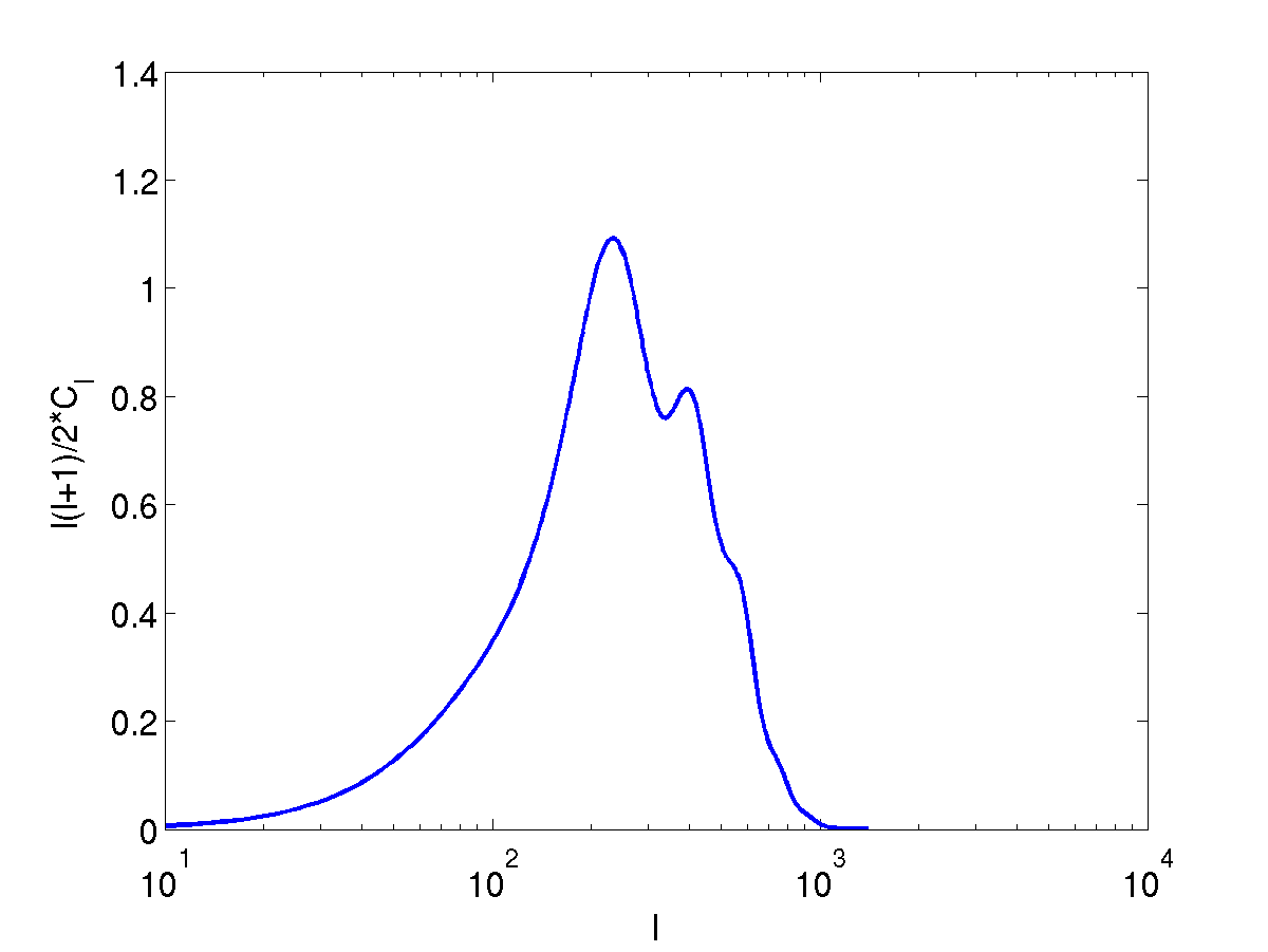
Figure 1: Coefficients $C_{l}$ using the CMBSimple.

Let us assume now that these values of the coefficients $C_{l}$ are the observed values, and that we know exactly every cosmological parameter other than the spectral coefficients of the power spectrum ${\mathcal{P}}_{\mathcal{R}}(\kappa)$. We will perform the inverse computation, in which the spectral coefficients $n_{s},\alpha_{s}$ and possibly $\beta_{s},\gamma_{s},\delta_{s}$ are given the values that minimize either the residue (10), or that in (11). As the value of every other cosmological parameter is known, the optimization problem is now simple enough so that several standard algorithms such as MCMC, the Levenberg-Marquardt method for nonlinear regression or the simplex search method for minimization of the residue function (Press 1992) will converge to the sought best parameter fit.

Table 4 shows in its columns the results of 3 computations, finding the spectral parameters in a power spectrum that has terms up to $\alpha_{s}$, resp. up to $\beta_{s}$, up to $\delta_{s}$, by computing the coefficients $C_{l}$ for $l$ ranging from 10 to 1400 with step 10 according to Eq. (8) for each choice of spectral parameter value and minimizing the residue in formula (11) in the comparison with the ”observed” values. Minimizing the residue (10) yields roughly the same values for the spectral parameters.

$\downarrow$ param. computation $\rightarrow$	correct value	fit up to $\alpha_{s}$	up to $\beta_{s}$	up to $\delta_{s}$
$n_{s}$	0.96	0.9374	0.9708	0.9653
$\alpha_{s}$	$6\cdot 10^{-3}$	$1.14\cdot 10^{-2}$	$1.34\cdot 10^{-3}$	$2.64\cdot 10^{-3}$
$\beta_{s}$	$2\cdot 10^{-4}$		$1.12\cdot 10^{-3}$	$1.6\cdot 10^{-3}$
$\gamma_{s}$	$5\cdot 10^{-5}$			$-1.95\cdot 10^{-4}$
$\delta_{s}$	$8\cdot 10^{-6}$			$3.37\cdot 10^{-5}$

Table 4:

The results in Table 4 are strikingly similar to those in Table $3$. Our recurring topic in this section of the paper perfectly interprets the results of these spectral parameter determinations:

• In each computation, the highest order parameter that has been used for fitting the $C_{l}$ coefficients has been overestimated: by a factor of 1.9 in the computation up to $\alpha_{s}$, by a factor of 5.5 in the computation up to $\beta_{s}$, by a factor of 4.2 in the computation up to $\delta_{s}$.

• The second to highest order parameter has been underestimated in each computation, even changing sign for $\gamma_{s}$ in the last one, as a correction to the overestimation of the highest order term.

• As the computation of spectral parameters assumes a polynomial function $\ln{\mathcal{P}}_{\mathcal{R}}(\kappa)$ with coefficients up to higher order, the determination of the lowest order coefficients $n_{s},\alpha_{s}$, becomes more accurate. This is indeed a trend, but the greater complexity and propagation of measurement errors of the residue minimization as the number of parameters grows do not allow in practice a scheme in which $\ln{\mathcal{P}}_{\mathcal{R}}(\kappa)$ is determined with coefficients up to a high order, so as to obtain reliable values for the low order coefficients.

These conclusions hold for the best fit solution to the optimization problem of minimizing the residue. Therefore they hold for any procedure that may be employed to find the best fit parameters (MCMC, …).

5 Conclusions

Single field slow rolling inflaton models do not fit well the computation of the spectral parameters of the temperature power spectrum of the CMB radiation by the Planck collaboration (Ade et al. 2013, 2015).

Of the 49 models examined in the study (Martin, Ringeval & Vennin 2013), only the following 8 can, with any choice of parameters for the model, yield values for the spectral parameters $n_{s},\alpha_{s},\beta_{s}$ at a distance of less than $1.8\sigma$ from the values given by (Ade et al. 2013, 2015). The models that do not lie outside this 92.8% confidence interval are RpI, KMIII, LMI, BSUSYBI, SSBI, TI, GMLFI, CNDI (model details and references in 3.2).

The ultimate reason for this poor fit is that the reported values for the parameters $n_{s}-1,\alpha_{s},\beta_{s}$ does not follow the hierarchy of sizes forecast by the slow roll theory, according to which these parameters ought to have decreasing order of magnitude. The running of the running $\beta_{s}$ reported by PLANCK2015 has a size $O(10^{-2})$ which is so large that most of the tested inflaton models cannot furnish values within 1.8 standard deviations of the expected value.

This discrepancy between the values for the spectral parameters determined by the Planck collaboration and the expected slow roll size hierarchy for them can arguably be due to lack of accuracy in the determination of these values, specially for the higher order parameters. Such lack of accuracy would mean that the models that do not match the used determinations of $\alpha_{s},\beta_{s}$ are not disproved by this mismatch.

In this work we identify a bias in the method that has been used for the computation of the values of the spectral parameters, which results in a systematic overestimation of the highest order one. The bias is a migration of, and very close to, a classical bias of regression (i.e., minimization of residue) fitting: if one tries to fit a polynomial of too low degree to values of a function that actually grows faster, no matter what the procedure for finding the better fit is, it will result in a polynomial with an exaggerated value for the magnitude of the leading term.

While vastly more powerful than their predecessors, the probabilistic (Bayesian, MCMC, …) methods currently used to fit the value of spectral parameters following a Gaussian distribution in a model ultimately choose the fit that minimizes the residue, and inherit this bias.

Removal of this bias will be necessary to judge if single field, slow roll inflation models match the increasingly refined measuremnents of the CMB, or if sophistications such as scalar electrodynamics and $SU(5)$ RG-improved potentials (Elizalde, Odintsov, Pozdeeva & Vernov 2014), warm inflation (Berera 1995; Bastero-Gil 2014), multiple fields, a breakdown in the slow roll regime (Easther & Peiris 2006; Wan et al. 2014), or a completely different paradigm such as the Matter Bounce Scenario can be contemplated (Cai, Brandenberger & Zhang 2009, 2011; Cai 2014).

The authors have little hope that spectral parameters such as the running $\alpha_{s}$, the running of the running $\beta_{s}$, and the higher order coefficients of the power spectrum ${\mathcal{P}}_{\mathcal{R}}$ can be computed reliably from experimental observations. These invariants are derivatives of increasingly high order of the function’s logarithm at a pivot value $k=k_{*}$, and derivatives are notoriously hard to compute in the presence of noise (i.e., experimental errors and slow roll approximations) in the data. Indeed, schemes to compute these spectral parameters up to a high order by residue minimization so as to get a reliable determination of the lowest order ones fail because of the propagation of the noise throughout the computation.

An approach that seems more promising is to avoid these spectral parameters: the Mukhanov-Sasaki equations

$$v_{k}^{\prime\prime}+\left(k^{2}-\frac{z^{\prime\prime}}{z}\right)v_{k}=0,\qquad z=a\frac{\varphi^{\prime}}{\mathcal{H}}$$ (14)

together with the conservation and Friedmann equations

$$\ddot{\varphi}+3H\varphi+V_{\varphi}=0,$$ (15)

$$H=\frac{1}{\sqrt{3}}\sqrt{\frac{\dot{\varphi}^{2}}{2}+V(\varphi)},$$ (16)

determine the power spectrum ${\mathcal{P}}_{\mathcal{R}}$ once the parameters $(\varphi_{0},\dot{\varphi}_{0})$ on which the background depends as initial conditions for the conservation equation, and those required by the potential $V(\varphi)$, have been set. The coefficients $C_{l}$ can then be determined from ${\mathcal{P}}_{\mathcal{R}}$, and one can look for the values of the background and potential parameters yielding a power spectrum ${\mathcal{P}}_{\mathcal{R}}$ that minimizes the residue (11), or (10). This is a computationally intensive task, so an efficient residue minimization scheme such as MCMC seems appropiate. The fit of particular models to the observations of $C_{l}$ can be judged, e.g. by means of Bayesian techniques, through these background and potential parameters. The authors believe that this approach merits further investigation.

This investigation has been supported in part by MINECO (Spain), projects MTM2011-27739-C04-01, and MTM2012-38122-C03-01.

References

- [1] Ade P.A.R. et al., 2014, Astronomy and Astrophysics, 571, A22
- [2] Ade P.A.R. et al., 2015, preprint (arXiv:1502.02114)
- [3] Albrecht A., Brandenberger R.H., 1986, Phys. Rev. D, 31, 1225
- [4] Barrow J.D., and Nunes N.J., 2007, Phys. Rev. D, 76, 043501
- [5] Bassett B.A., Tsujikawa S., Wands D., 2006, Rev.Mod.Phys., 78, 537 (2006)
- [6] Bastero-Gil M.et al., 2014, JCAP, 1410, 053
- [7] Baumann D., 2011, The Physics of Inflation, ICTS course
- [8] Berera A., 1995, Phys. Rev. Lett., 75, 3218
- [9] Binetruy P., Dvali G., 1996, Phys.Lett. B, 388, 241
- [10] Cai Y.F. et al., 2009, Phys. Rev. D 80, 023511
- [11] Cai Y.F., Brandenberger R. and Zhang X., 2011, JCAP, 1103, 003
- [12] Cai Y.F., 2014, SCIENCE CHINA: Phys. Mech. Astr., 57, 1414
- [13] Christensen N., Meyer R., 2000, preprint (arXiv:0006401)
- [14] Conlon J.P, Quevedo F., 2006, JHEP, 0601, 146
- [15] Dodelson S., Kinney W.H., Kolb E.W., 1997, Phys.Rev. D 56, 3207
- [16] Dudas E. et al., 2012, preprint (arXiv:1202.6630)
- [17] Easther R. and Peiris H., 2006, JCAP, 0609, 010
- [18] Elizalde E.,Odintsov S.D., Pozdeeva E.O., Vernov S.Y., 2014, Phys. Rev. D 90, 084001
- [19] Giannantonio T., Komatsu E., 2015, Phys. Rev. D, 91, 023506
- [20] E. Halyo , 1996, Phys.Lett. B, 387, 43
- [21] Hodges H, Blumenthal G, 1999, Phys. Rev. D, 42, 3329
- [22] Hu B. and O’Connor D., 1986, Phys.Rev. D, 34, 2535
- [23] Huang Q.G., 2006, JCAP, 0611, 004
- [24] Kinney W.H., Riotto A., 1998, Phys.Lett. B, 435, 272
- [25] Kinney W.H., Riotto A., 1999, Astropart. Phys., 10, 387
- [26] Kurki-Suonio H., 2005, Cosmology I & II. Lecture notes, Univ. Helsinki
- [27] Lee S., Nam S., 2011, Int. J. Mod. Phys. A, 26, 1073
- [28] Martin J., Ringeval C., 2004, Phys.Rev. D, D69, 083515
- [29] Martin J., Ringeval C., Vennin V., 2013, preprint (arXiv:1303.3787)
- [30] Martin J., Ringeval C., Trotta R. and Vennin V., 2014, JCAP, 1403, 039
- [31] Pajer E., 2008, JCAP, 0804, 031
- [32] Parsons P., J. D. Barrow J.D., 1995, Phys.Rev. B, 51, 6757
- [33] Press W.H. et al., 1992, Numerical Recipes in C. The Art of Scientific Computing. 2nd Ed., Cambridge U.P.
- [34] Seljak U., Zaldarriaga M., 1996, Astrophys. J., 469, 437
-
[35]
De Felice A., and Tsujikawa S., 2010, Living Rev.Rel., 13, , 3 (2010)
Nojiri S., Odintsov S.D., 2011, Phys.Rept., 505, 59 - [36] Verde L. et al., 2003, Astrophys. J. Supp. Series, 148, 195 (2003)
- [37] Wan Y. et al., 2014 , Phys. Rev. D, 90, 023537 (2014)