Abstract

We carry out a systematic qualitative analysis of the two quadratic schemes of generalized oscillators recently proposed by C. Quesne [J.Math.Phys.56,012903 (2015)]. By performing a local analysis of the governing potentials we demonstrate that while the first potential admits a pair of equilibrium points one of which is typically a center for both signs of the coupling strength $\lambda$, the other points to a centre for $\lambda<0$ but a saddle $\lambda>0$. On the other hand, the second potential reveals only a center for both the signs of $\lambda$ from a linear stability analysis. We carry out our study by extending Quesne’s scheme to include the effects of a linear dissipative term. An important outcome is that we run into a remarkable transition to chaos in the presence of a periodic force term $f\cos\omega t$.

Qualitative analysis of certain generalized classes of quadratic oscillator systems

PACS: 45.20.Jj, 45.50.Dd, 05.45.-a

1 Introduction

Nonlinear autonomous differential equations of second order have proved to be of much interest in the investigation of dynamical systems and nonlinear analysis [1, 2, 3, 4, 5, 6, 7]. Consider a typical one belonging to quadratic Liénard class as given by

$$\ddot{x}+r(x)\dot{x}^{2}+s(x)=0$$ (1)

where an overdot indicates a derivative with respect to the time variable $t$ and $r(x)$ and $s(x)$ are two continuously differentiable functions of the spatial coordinate $x$. The following specific forms of $r$ and $s$ which are odd functions of $x$, namely

$$r(x)=-\frac{\lambda x}{1+\lambda x^{2}},\quad g(x)=\frac{\alpha^{2}x}{1+\lambda x^{2}},\quad\lambda>0$$ (2)

where $\alpha$ and $\lambda$ are nonzero real numbers, lead to a nonlinear equation defined by

$$(1+\lambda x^{2})\ddot{x}-\lambda x\dot{x^{2}}+\alpha^{2}x=0$$ (3)

The Lagrangian relevant to (3)

$$L=\frac{1}{2}\frac{1}{1+\lambda x^{2}}(\dot{x^{2}}-\alpha^{2}x^{2})$$ (4)

was studied by Mathews and Lakshmanan (ML) [8] long time ago in the search of a one-dimensional analogue of some quantum field theoretic model. One can observe that (4) speaks of a $\lambda$-dependent deformation of the standard harmonic oscillator Lagrangian. Cariñena et al [9] also pointed out that the kinetic term in this Lagrangian is invariant under the tangent lift of the vector field $X_{x}(\lambda)=\sqrt{1+\lambda x^{2}}\frac{\partial}{\partial x}$.

The corresponding Hamiltonian represents a position-dependent effective mass system guided by the mass function of the specific type $m(x)=\frac{1}{1+\lambda x^{2}}$. In the literature dynamics of several types of nonlinear systems have been found to be influenced by a position-dependent effective mass [10, 11, 12, 13, 14, 15, 16, 17, 18]. From a physical point of view problems of position-dependent effective mass have relevance in describing the flow of electrons in problems of compositionally graded crystal, quantum dots and liquid crystals [19, 20, 21].

As is well known the nonlinear dynamics described by (3) admits, in particular, a periodic solution for $x(t)$ given by the simple harmonic form

$$x(t)=Asin(\omega t+\phi)$$ (5)

but with the restriction that the frequency $\omega$ is related to the amplitude $A$ by the constraint $\omega^{2}=\frac{\alpha^{2}}{1+\lambda A^{2}}$. The amplitude thus depends on the frequency.

From the form of the Lagrangian (4) it is easy to identify the corresponding potential $V(x)$ as given by

$$V(x)=\frac{1}{2}\frac{\alpha^{2}x^{2}}{1+\lambda x^{2}}.$$ (6)

Recently Quesne [22] extended the above potential to two different types of generalizations by introducing a two-parameter deformation by bringing in an additional phenomenological parameter $\beta$ in the following manner:

$$(a)\quad V_{I}=\frac{1}{2}\frac{\alpha^{2}x^{2}-2\beta x}{1+\lambda x^{2}}$$ (7)

$$(b)\quad V_{II}=\frac{1}{2}\frac{\alpha^{2}x^{2}-2\beta x\sqrt{1+\lambda x^{2}}}{1+\lambda x^{2}}$$ (8)

while keeping the kinetic part of (4) unchanged. The respective Euler-Lagrange equations that follow from (7) and (8) read

$$(1+\lambda x^{2})\ddot{x}-\lambda x\dot{x}^{2}+\alpha^{2}x-\beta{(1-\lambda x^{2})}=0$$ (9)

$$(1+\lambda x^{2})\ddot{x}-\lambda x\dot{x}^{2}+\alpha^{2}x-\beta\sqrt{{(1+\lambda x^{2})}}=0$$ (10)

Let us emphasize that the functional form corresponding to $s(x)$ in the above equations is not odd but of a mixed type consisting of a term that is odd and a term that is even. With an extra parameter $\beta$ at hand, quite expectedly, the potentials $V_{I}$ and $V_{II}$ allow dealing with richer behaviour patterns of the solutions of the corresponding Euler-Lagrange equations than the ones provided by (4) for the ML case. One of the guiding factors in this regard is the sign of the deformation parameter $\lambda$ that corresponds to different asymptotic behaviour of the two potentials $V_{I}$ and $V_{II}$ and the locations of the minimum for the latter. The first integral of the Euler-Lagrange equation when suitably confronted with the integration constant and the underlying discriminant also give crucial restrictions on the domains of the energy of the system for a physically viable solution.

In this paper we interpret the generalized nonlinear oscillators that are guided by $V_{I}$ and $V_{II}$ as examples of dynamical systems and perform a qualitative analysis to determine some interesting local properties for them. We also take up the issue of chaos in the presence of a periodic force term $f\cos\omega t$ for both the systems by fine-tuning some of the coupling parameters.

2 Local analysis of the potential $V_{I}(x)$

Let us rewrite the Euler-Lagrange equation in the presence of $V_{I}$ as the following system of coupled equations

$$\dot{x} = y$$

$$\dot{y} = \frac{\lambda xy^{2}}{1+\lambda x^{2}}\quad-\frac{\alpha^{2}x}{1+\lambda x^{2}}\quad+\frac{\beta(1-\lambda x^{2})}{1+\lambda x^{2}}.$$ (11)

The resulting fixed points are readily identified to be located at the points $(x_{1}^{*},0)$ and $(x_{2}^{*},0)$ where

$$x_{1,2}^{*}=(-\alpha^{2}\pm\sqrt{\alpha^{4}+4\lambda\beta^{2}})/2\lambda\beta.$$ (12)

The positivity of the discriminant leads to the restriction $\lambda>-\alpha^{4}/4\beta^{2}$.

Evaluating now the Jacobian matrix we obtain at the fixed points

$$J|_{(x_{1,2};0)}=\left(\begin{array}[]{cc}0&1\\ A_{21}&0\\ \end{array}\right)$$ (13)

where

$$A_{21}=(-\alpha^{2}+\lambda\alpha^{2}x_{c}^{2}-4\lambda\beta x_{c})/(1+\lambda x_{c}^{2})^{2}$$ (14)

and $x_{c}=x_{1,2}^{*}$.

For $\lambda>0$, the respective eigenvalues of $J$ at $x_{1}^{*}$ and $x_{2}^{*}$ are

$$\pm i\sqrt{\frac{2\lambda\beta^{2}}{\sqrt{D}-\alpha^{2}}},\;\;\pm\sqrt{\frac{2\lambda\beta^{2}}{\sqrt{D}+\alpha^{2}}}$$ (15)

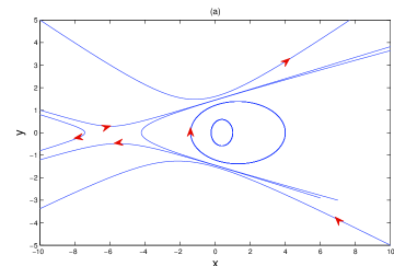
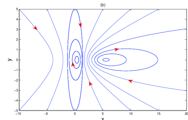
Figure 1: Phase diagram of the system (2 Local analysis of the potential $V_{I}(x)$) for (a)$~{}\lambda=0.5~{}$, (b)$~{}\lambda=-0.5~{}$ with $~{}\beta=0.34~{}$, $~{}\alpha=1.0~{}$.

where $D=\alpha^{4}+4\beta^{2}\lambda>0$ implying $\sqrt{D}>\alpha^{2}$. We therefore conclude that the point $(x_{1}^{*},0)$ is a center while the other one, namely $(x_{2}^{*},0)$, is a saddle point. The phase diagram of the system (2 Local analysis of the potential $V_{I}(x)$) is plotted in Figure 1a taking the parameter values $\lambda=0.5$ , $~{}\beta=0.34~{}$ $~{}\alpha=1.0~{}$.

In the case of $\lambda<0$ the two eigenvalues of the Jacobian matrix (13) at $x_{1}^{*}$ and $x_{2}^{*}$ are given by

$$\pm i\sqrt{\frac{-2\lambda\beta^{2}}{\alpha^{2}-\sqrt{D}}},\;\;\pm i\sqrt{\frac{-2\lambda\beta^{2}}{\alpha^{2}+\sqrt{D}}}$$ (16)

where $D=\alpha^{4}+4\beta^{2}\lambda>0$. $~{}\alpha^{2}>\sqrt{D}~{}$ as $-\alpha^{4}/4\beta^{2}\leq\lambda<0$.

Here too the equilibrium points $(x_{1}^{*},0)$ and $(x_{2}^{*},0)$ correspond to centers since the eigenvalues of the Jacobian matrix are purely imaginary conjugate pairs for $\lambda<0$. Figure 1b represents the phase portrait of the system (2 Local analysis of the potential $V_{I}(x)$) for $\lambda=-0.5$ , $~{}\beta=0.34~{}$ $~{}\alpha=1.0~{}$. The Figure 1a and Figure 1b are consistent.

3 Local analysis of the potential $V_{II}(x)$

The dynamical system for the potential $V_{II}(x)$ is described by the following set of equations

$$\dot{x} = y$$

$$\dot{y} = \frac{\lambda xy^{2}}{1+\lambda x^{2}}\quad-\frac{\alpha^{2}x}{1+\lambda x^{2}}\quad+\frac{\beta\sqrt{1+\lambda x^{2}}}{1+\lambda x^{2}}.$$ (17)

The two equilibrium points correspond to $(x_{1}^{*},0)$ and $(x_{2}^{*},0)$ where

$$x_{1,2}^{*}=\pm\frac{\beta}{\sqrt{\alpha^{4}-\lambda\beta^{2}}}$$ (18)

subject to the positivity condition $\alpha^{4}-\lambda\beta^{2}>0$ i.e. $\lambda<\alpha^{4}/\beta^{2}$. At the equilibrium points the Jacobian matrix takes the form

$$J|_{(x_{1,2};0)}=\left(\begin{array}[]{cc}0&1\\ A_{21}&0\\ \end{array}\right)$$ (19)

where $A_{21}$ is given by

$$A_{21}=\frac{\alpha^{2}(\lambda x_{c}^{2}-1)-\lambda\beta x_{c}\sqrt{1+\lambda x_{c}^{2}}}{(1+\lambda x_{c}^{2})^{2}}$$ (20)

and $x_{c}$ stands for $x_{c}=x_{1,2}^{*}$ .

The eigenvalues of $J$ represent a pair of degenerate conjugate complex quantities namely,

$$\pm\frac{i(\alpha^{4}-\lambda\beta^{2})}{\alpha^{3}},~{}\pm\frac{i(\alpha^{4}-\lambda\beta^{2})}{\alpha^{3}}$$ (21)

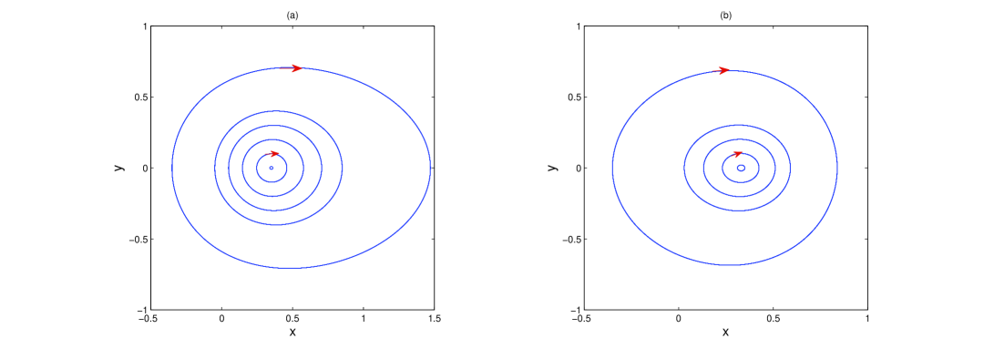
Figure 2: Phase portrait of the system (19) for (a)$~{}\lambda=0.5~{}$ ,(b) $~{}\lambda=-0.5~{}$; with $~{}\beta=0.34~{}$, $~{}\alpha=1.0~{}$.

While the linear stability analysis indicates the nonhyperbolic nature of the fixed points, as is well known such tests are not always in conformity with the nonlinear analysis. Indeed, the numerical simulation of the nonlinear system of (3 Local analysis of the potential $V_{II}(x)$), as shown in Figure 2, confirms that the linear stability results correctly predict the behavior of one of the equilibrium points namely $x_{1}^{*}$ but it fails in the case of the other equilibrium point, $x_{2}^{*}$.

4 Inclusion of an external periodic forcing term

   It is of considerable interest to study the dynamics of systems (2 Local analysis of the potential $V_{I}(x)$) and (3 Local analysis of the potential $V_{II}(x)$), under the influence of the external periodic forcing in the presence of additional damping, so that the respective equation of motion become

$$(1+\lambda x^{2})\ddot{x}-\lambda x\dot{x}^{2}+\alpha^{2}x-\beta{(1-\lambda x^{2})}+\gamma\dot{x}=fcos(\omega t)$$ (22)

$${\mbox{and}~{}~{}}(1+\lambda x^{2})\ddot{x}-\lambda x\dot{x}^{2}+\alpha^{2}x-\beta\sqrt{{(1+\lambda x^{2})}}+\gamma\dot{x}=fcos(\omega t).$$ (23)

The above nonautonomous systems can be rewritten as the following three dimensional autonomous nonlinear dynamical systems respectively

$$\dot{x} = y$$

$$\dot{y} = \frac{\lambda xy^{2}-\gamma y}{1+\lambda x^{2}}\quad-\frac{\alpha^{2}x}{1+\lambda x^{2}}\quad+\frac{\beta(1-\lambda x^{2})}{1+\lambda x^{2}}+\frac{f\cos z}{1+\lambda x^{2}}$$ (24)

$$\dot{z} = \omega$$

and

$$\dot{x} = y$$

$$\dot{y} = \frac{\lambda xy^{2}-\gamma y}{1+\lambda x^{2}}\quad-\frac{\alpha^{2}x}{1+\lambda x^{2}}\quad+\frac{\sqrt{\beta(1+\lambda x^{2})}}{1+\lambda x^{2}}+\frac{f\cos z}{1+\lambda x^{2}}$$ (25)

$$\dot{z} = \omega$$

We have done numerical simulations of the system (4 Inclusion of an external periodic forcing term) only. The simulation results of the syatem (4 Inclusion of an external periodic forcing term) are qualitatively similar and hence not discussed.

5 Results and discussion

5.1 Case-I: No Dissipation ($\gamma=0$)

We start with the dynamics of the ML-model in the absence of dissipation. Thus we set $~{}\gamma=0~{}$ and consider a set of sample parameter values $~{}\lambda=-0.5~{}$, $~{}\alpha=2.0~{}$, $~{}\gamma=0.0~{}$, $~{}\omega=1.0~{}$, $~{}f=5.0~{}$ to plot the phase portrait in the $xy$-plane. It reveals the quasi-periodic nature of the system whose character survives for a wide range of inputs for the external periodic forcing term. In Figure 3 we have plotted the phase diagram in the $xy$ plane of the system (4 Inclusion of an external periodic forcing term) for the parameter values $~{}\lambda=-0.5~{}$, $~{}\alpha=2.0~{}$, $~{}\gamma=0.0~{}$, $~{}\omega=1.0~{}$, $~{}f=5.0~{}$ corresponding to the test values of $~{}\beta~{}$ as given by $~{}\beta=0.001~{}$, $~{}\beta=0.01~{}$ and $~{}\beta=0.1~{}$. These values of $~{}\beta~{}$ correspond to small and moderate departures from the ML-model. Figure 3a illustrates the case of $~{}\beta=0.001~{}$ while the Poincaré first return map of the same is plotted in Figure 3b. We observe that the first return map data lie on 3 smooth closed curves confirming the existence of the quasiperiodic behaviour of the system. The latter behavior persists for the choice of $~{}\beta=0.01~{}$ also. The phase diagram for $~{}\beta=0.1~{}$ keeping the other parameters fixed is exhibited in Figure 3c. However, the first return map as presented in Figure 3d shows a drastic change. The irregular scattering of points in the latter figure points to the existence of chaos in the system. We therefore observe the sensitivity of the system (4 Inclusion of an external periodic forcing term) to the choice of the $~{}\beta~{}$-values as evidenced by the transition from quasi-periodicity to chaos as the value of $~{}\beta~{}$ is changed from $~{}\beta=0.001~{}$ by two orders of magnitude.

Next we discuss for the system (4 Inclusion of an external periodic forcing term) the phase diagrams and those for Poincaré return maps for different values of forcing amplitude $~{}f~{}$ for the data set $~{}\lambda=-0.5~{}$, $~{}\alpha=2.0~{}$, $~{}\beta=0.1~{}$, $~{}\gamma=0.0~{}$, $~{}\omega=1.0~{}$. These are summarized in Figure 4. In Figure 4a we have plotted the phase portrait for $~{}f=0.0~{}$ and the corresponding Poincaré first return map is shown in Figure 4b. The existence of only one point in the Figure 4b proves the existence of periodic orbit in case of no external forcing. In Figure 4c the phase diagram of the system is presented for $~{}f=3.0~{}$ and the corresponding Poincaré first return map is given in Figure 4d. The return map data lie on smooth closed curves and hence confirms the existence of quasiperiodic behaviour of the system for $f=3.0$. We have plotted the phase portrait for $~{}f=5.0~{}$ in Figure 4e and the corresponding return map data are plotted in Figure 4f. The irregular set of points in the whole plane guarantee the existence of chaos in the system for $~{}f=5.0$. Therefore as in the previous case the increase of forcing amplitude also produces chaotic motion via the quasiperiodic route.

5.2  Case-II: Dissipative Case ($\gamma\neq 0$)

We now turn to the inclusion of the dissipation effects in the model (4 Inclusion of an external periodic forcing term). Towards this end we keep the following fixed sample values of $~{}\lambda=-0.5~{}$, $~{}\alpha=2.0~{}$, $~{}\beta=0.1~{}$, $~{}\omega=1.0~{}$ and $~{}f=5.0~{}$ and vary the dissipation parameter $\gamma$. We consider an assorted set of values for $\gamma$ ranging from very small to moderately large values. We represent in Figure 5a the phase portrait in the xy plane for $~{}\gamma=0.002~{}$ and the corresponding Poincaré map in the Figure 5b. We find a set of randomly distributed points that tells us about the chaotic character inherent in the system (4 Inclusion of an external periodic forcing term). Next for $~{}\gamma=0.02~{}$, from the phase portrait of system (4 Inclusion of an external periodic forcing term) plotted in the Figure 5c and corresponding Poincaré map in the Figure 5d, we notice a finite number of closed curves that confirm the existence of quasiperiodic oscillations. Figures 5e and 5f display the phase portrait and time evolution of the variable $y$ for an order of magnitude higher value of $~{}\gamma=0.1~{}$. Time evolution of the corresponding phase portrait of Figure 5f guarantees the presence of a periodic behaviour for $~{}\gamma=0.1~{}$. In Figure 6 we provide the bifurcation diagram of the variable $y$ with respect to the parameter $~{}\gamma~{}$. It is clear that, with the increase of dissipation, the system undergoes a transition from chaos to quasiperiodicity and then settles to a periodic behavior.

6 Summary

In this paper we studied the dynamical behavior of two quadratic schemes of generalized oscillators recently proposed by Quesne. We performed a local analysis of the governing potentials to demonstrate that while the first potential admits a typically center-like equilibrium point for both signs of the coupling strength $\lambda$, the second potential only admits to a centre for $\lambda<0$ but a saddle $\lambda>0$. The second potential however reveals, from a linear stability analysis, only a center for both the signs of $\lambda$. We have extended Quesne’s scheme to include the effects of a linear dissipative term and shown how inclusion of an external periodic force term changes the qualitative behavior of the underlying systems drastically leading to the possible onset of chaos.

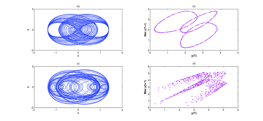
Figure 3: Phase portrait of the system (4 Inclusion of an external periodic forcing term) with $~{}\lambda=-0.5~{}$, $~{}\alpha=2.0~{}$, $~{}\gamma=0.0~{}$, $~{}\omega=1.0~{}$, f=5.0 for different value of $~{}\beta~{}$ (a) $~{}\beta=0.001~{}$, (c)$~{}\beta=0.1~{}$; (b) and (d) represent corresponding Poincare first return map.

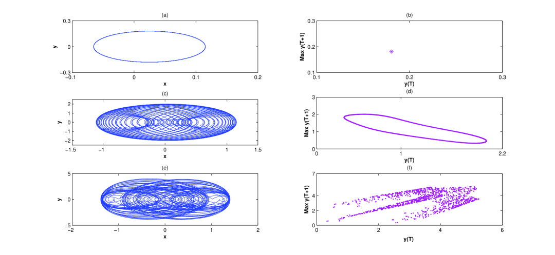
Figure 4: Phase portrait of the system (4 Inclusion of an external periodic forcing term) with $~{}\lambda=-0.5~{}$, $~{}\alpha=2.0~{}$, $~{}\beta=0.1~{}$, $~{}\gamma=0.0~{}$, $~{}\omega=1.0~{}$ for different value of $f$ (a) f=0.0, (c) f=3.0, (e) f=5.0 ; (b),(d) and (f) represent corresponding first return map.

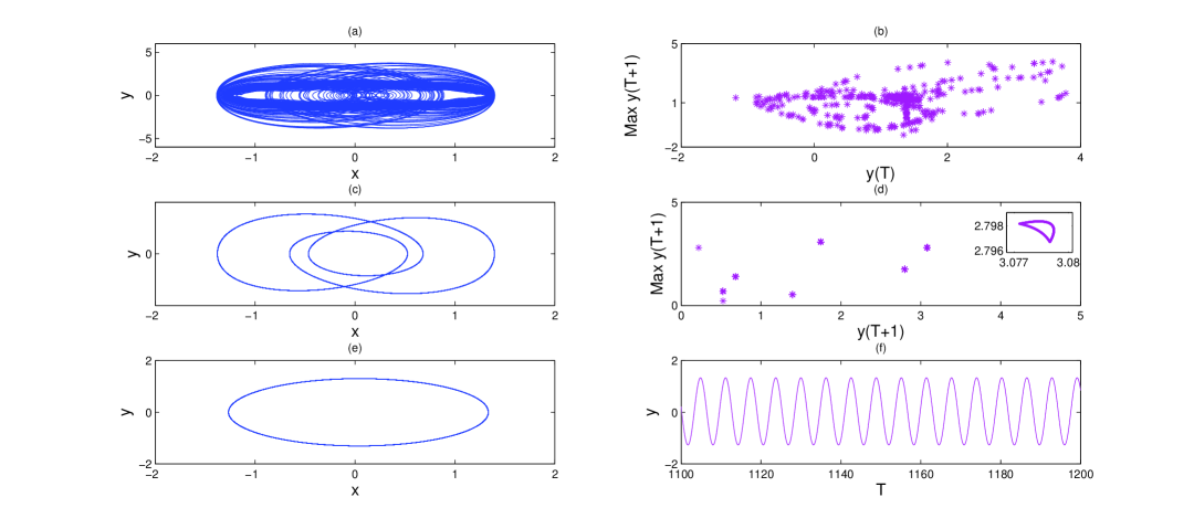
Figure 5: Phase portrait of the system (4 Inclusion of an external periodic forcing term) with $~{}\lambda=-0.5~{}$, $~{}\alpha=2.0~{}$, $~{}\beta=0.1~{}$, $~{}\omega=1.0~{}$ and $~{}f=5.0~{}$ for different value of $~{}\gamma~{}$ (a) $~{}\gamma=0.002~{}$,(c) $~{}\gamma=0.02~{}$, (e) $~{}\gamma=0.1~{}$; (b),(d) represent corresponding first return map; (f) corresponding time series

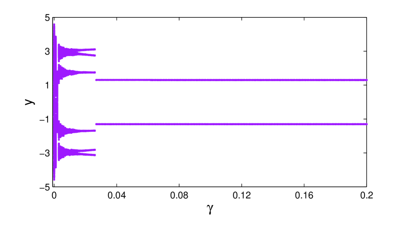
Figure 6: Bifurcation diagram of y with respect to parameter $~{}\gamma~{}$ of the system (4 Inclusion of an external periodic forcing term) with $~{}\lambda=-0.5~{}$, $~{}\alpha=2.0~{}$, $~{}\beta=0.1~{}$, $~{}\omega=1.0~{}$ and $~{}f=5.0~{}$.

References

- [1] J. Guckenheimer and P. Holmes, Nonlinear oscillations, dynamical systems and bifurcations of Vector Fields, Springer-Verlag, New York (1983).
- [2] M. Tabor, Chaos and integrability in nonlinear dynamics: An introduction, John Wiley and Sonc. Inc, New York (1989).
- [3] A. H. Nayfeh and D. T. Mook, Nonlinear oscillations, John Wiley Sons, New York (1995).
- [4] S. Wiggins, Introduction to Applied Nonlinear Dynamical Systems and Chaos, Springer-Verlag, New York (2003).
- [5] M. Lakshmanan and S. Rajasekar, Nonlinear dynamics: Integrability chaos and patterns, Springer-Verlag, New York (2003).
- [6] M.Lakshmanan and V.C. Chandrasekar, Eur. Phys. J - ST 222, 665 (2013).
- [7] A.K.Tiwari, S.N.Pandey, M.Senthivelan and M.Lakshmanan, J. Math. Phys. 54, 053506 (2013).
- [8] P.M.Mathews and M. Lakshmanan, Q. Appl. Maths. 32,215 (1974).
- [9] J F Cariñena, M F Rañada and M Santander, Two important examples of nonlinear oscillators in Procs. of the 10 Int. Conf. in in Modern Group Analysis, Larnaca, Chipre, edited by N.H. Ibragimov, Ch. Sophocleous and P. A. Damianou (University of Cyprus, Larnaca Cyprus, 2005), pp.39-46; also e print arXiv: math-ph 0505028; Rep. Math. Phys. 54, 285 (2004).
- [10] J F Cariñena, M F Rañada and M Santander, Ann Phys. 322, 2249 (2007).
- [11] M.F.Rañada, J.Math.Phys.54,093502 (2013).
- [12] S Cruz y Cruz, J Negro and L M Nieto Phys. Letts. A369, 400 (2007), S Cruz y Cruz and O Rosas-Ortiz J Phys. A: Math. Theor. 42, 185205 (2009), S Cruz y Cruz and O Rosas-Ortiz Lagrange equations and Spectrum generators algebras of mechanical systems with position-dependent mass arXiv: 1208.2300.
- [13] B Bagchi, S Das, S Ghosh and S Poria, J. Phys. A Math: Theor. 46 032001 (2013).
- [14] O. Mustafa, J.Phys.A: Math. Theor.46,368001 (2013).
- [15] M.Khan and T. Shah, Nonlinear Dynamics 76, 377 (2014)
- [16] A Ghose Choudhury, P Guha and B Khanra, J. Math. Anal. Appl. 360 no. 2, 651-664 (2009).
- [17] D.Ghosh and B.Roy, Ann.Phys.353,222 (2015).
- [18] A.Schulze-Halberg and J.R.Morris, Eur.Phys.J.Phys.128,54 (2013).
- [19] M R Geller and W Kohn, Phy. Rev. Lett. 70, 3103 (1993).
- [20] L Serra and E Lipparini, Europhys. Lett. 40, 667 (1997).
- [21] M Barranco, M Pi, S. M. Gatica, E S Herńandez and J. Navarro, Phys. Rev. B56, 8997 (1997).
- [22] C. Quesne, J.Math.Phys.56,012903 (2015).