Off-trail SUSY

Abstract:

We present two distinct topics:
I) We describe the propagation of a spin-3/2 state in a background which preserves invariance under space translations and rotations but not under Lorentz boost transformations. We start by building a generalisation of the Volkov-Akulov Lagrangian for a goldstino in a fluid. A super-Higgs mechanism leads to the modified Rarita-Schwinger Lagrangian describing a slow gravitino. We identify the physical propagating degrees of freedom and derive the corresponding equations of motion. This includes some new results.
II) Fake Split Supersymmetry Models are proposed to alleviate some of the problems of the original Split SUSY. In particular it is no more necessary to restrict to a Mini-Split scenario as higher values of the supersymmetry breaking scale (Mega-Split) are now allowed. The FSSM relies on swapping the higgsinos for new states in identical gauge group representations but different Yukawa couplings.

1 Introduction

We discuss here two topics. The first is an attempt to combine Lorentz symmetry breaking with supersymmetry in flat space-time. It is presented in section 2. The second concerns the possibility with having the largest possible SUSY breaking scale and it is the subject of section 3.

2 The slow gravitino and super-Higgs mechanism in fluids

The first part deals with study of a modified spin-3/2 Rarita-Schwinger Lagrangian [1] with two parameters, one dimension-full for the mass and the other dimensionless parameterising the Lorentz-symmetry breaking. This Lagrangian has a rich structure and can be studied per se as done in [2]. The gravitino exhibits an interesting feature: its longitudinal mode ($\pm 1/2$ helicities) has an effective speed of light smaller than the one appearing in the equation of motion of the transverse modes ($\pm 3/2$ helicities); thereof we call it slow gravitino. This phenomenon is common in spin-3/2 propagation on curved backgrounds [3, 4, 5, 6, 7].

Extensions of massive spin-3/2 Lagrangian that are free of the Velo-Zwanziger problem [8] (i.e loss of causality) can be constructed through a super-Higgs mechanism. This is the case for our Lagrangian: it describes the generation of a mass term for a goldstino appearing when SUSY is broken by a fluid background.

Supersymmetry is broken by temperature [9] and is not restored at any non-zero value. This is not surprising given that the bosons and fermions obey different statistics. However, the spontaneous or explicit nature of the breaking remained subject of confusion. Based on the fact that fermions have anti-periodic boundary conditions in the imaginary time, it was argued that there is no massless fermionic mode and that supersymmetry was explicitly broken [10]. However, working in the real time formalism, it was found in [11, 12] that there is a massless goldstino and supersymmetry is broken spontaneously. These results seem conflicting and have lead to a lot of debate in the literature. It was later traced back to two problems with the imaginary-time formalism: the first is that the study of linear response requires an analytical continuation to Minkowski space that is difficult to perform in the Fourier space and the second is that the imaginary-time breaks explicitly Lorentz covariance. Working in the real time formalism, it was possible to establish a Ward identity [12], to show the presence of a Goldstone fermion excitation and to identify the latter in certain cases with composite bilinear boson-fermion operators [13]. Later, the temperature goldstino has been called phonino [14] and has been subject to further studies (see for example [15, 16, 17, 18]). The only feature of the phonino that is relevant for this work is that it has a non-relativistic kinetic term, dressed by the stress-energy tensor of the fluid [19], which involves the derivative $T^{\mu\nu}{{\gamma}^{\ \!\!}}_{\mu}\partial_{\nu}$. The phonino is expected to acquire a mass through its interaction with the gravitino.

2.1 Alkulov-Volkov lagrangian for the phonino

The usual (Lorentz invariant) Alkulov-Volkov (AV) Lagrangian is given by:

$$\mathcal{L}~{}=-\frac{1}{2}f^{2}\ \det(W_{\mu}^{\phantom{\mu}\nu})$$ (2.1)

where $f$ is a constant parameter and

$$W_{\mu}^{\phantom{\mu}\nu}~{}=~{}\delta_{\mu}^{\phantom{\mu}\nu}+\frac{\bar{G}}{f}{{\gamma}^{\ \!\!}}_{\mu}\partial^{\nu}(\frac{G}{f})\ .$$

This Lagrangian has been chosen such that under the supersymmetry transformation of constant parameter $\epsilon$

$$\delta(\frac{G}{f})~{}=~{}\epsilon+\xi^{\mu}\partial_{\mu}(\frac{G}{f}) \xi^{\mu}~{}=~{}\bar{\epsilon}{{\gamma}^{\ \!\!}}^{\mu}\frac{G}{f}\ ,$$ with (2.2)

we have $\delta(W_{\mu}^{\phantom{\mu}\nu})=\partial^{\nu}\xi_{\rho}W_{\mu}^{\phantom{\mu}\rho}+\xi^{\rho}\partial_{\rho}W_{\mu}^{\phantom{\mu}\nu}\ ,$ and

$$\delta(\mathcal{L})~{}=~{}-\frac{1}{2}f^{2}\partial_{\mu}[\xi^{\mu}\det(W_{\rho}^{\phantom{\sigma}\sigma})]\ .$$

The Lagrangian (2.1) is therefore invariant up to total derivatives under the non-linear transformation (2.2). Expending (2.1) at first order in $G^{2}$, we obtain

$$\mathcal{L}~{}=~{}-\frac{1}{2}f^{2}-\frac{1}{2}\bar{G}{{\gamma}^{\ \!\!}}^{\mu}\partial_{\mu}G+\mathcal{O}(G^{4})\ .$$ (2.3)

The main new feature of the phonino is that instead of (2.3), the kinetic term has a non-Lorentz-invariant form $T^{\mu\nu}{{\gamma}^{\ \!\!}}_{\mu}\partial_{\nu}$. Defining $T$ or normalisation factor, the non-linear Lagrangian yielding this is given by:

$$\mathcal{L}~{}=~{}-\frac{1}{2}f^{2}\ \det\left[\delta_{\mu}^{\phantom{\mu}\nu}-\frac{\bar{G}}{f}\frac{T_{\mu\rho}{{\gamma}^{\ \!\!}}^{\rho}}{T}\partial^{\nu}(\frac{G}{f})\right]=-\frac{1}{2}f^{2}+\frac{1}{2}\bar{G}\frac{T^{\mu\nu}}{T}{{\gamma}^{\ \!\!}}_{\mu}\partial_{\nu}G+\mathcal{O}(G^{4})\ ,$$ (2.4)

with the modified non-linear supersymmetry transformations,

$$\delta(\frac{G}{f})~{}=~{}\epsilon+\xi^{\mu}\partial_{\mu}(\frac{G}{f}) \xi^{\mu}~{}=~{}-\bar{\epsilon}\frac{T^{\mu\rho}{{\gamma}^{\ \!\!}}_{\rho}}{T}\frac{G}{f}\ .$$ with (2.5)

It is straightforward to verify that (2.4) transforms as a total derivative under (2.5).

2.2 Super-Higgs mechanism in a fluid with curved background

2.2.1 Perfect fluid in curved background

To leading order in derivatives, the supergravity Lagrangian including the graviton, gravitino and goldstino fields is given by

$$\mathcal{L}~{}=~{}\frac{1}{2}e\left[\mathcal{L}_{\textrm{gravitino}}+\mathcal{L}_{\textrm{phonino}}+\mathcal{L}_{\textrm{mixing}}\right]+\mathcal{L}_{\textrm{f}}\ ,$$ (2.6)

where $e$ is the square root of the metric determinant and

$$\mathcal{L}_{\textrm{gravitino}} ~{}=~{}R-\bar{\psi}_{\mu}{{\gamma}^{\ \!\!}}^{\mu\nu\rho}\nabla_{\nu}\psi_{\rho}$$

$$\mathcal{L}_{\textrm{phonino}} ~{}=~{}\bar{G}\frac{T^{\mu\nu}}{T}{{\gamma}^{\ \!\!}}_{\mu}\nabla_{\nu}G$$

$$\mathcal{L}_{\textrm{mixing}} ~{}=~{}-\sqrt{2}\frac{T^{\mu\nu}}{\sqrt{T}M_{P}}\bar{G}{{\gamma}^{\ \!\!}}_{\mu}\psi_{\nu}\ .$$

This Lagrangian transforms as a total derivative under the linear transformations :

$$\begin{cases}\delta e_{\mu}^{a}&=~{}\frac{1}{2}M_{P}\bar{\epsilon}{{\gamma}^{\ \!\!}}^{a}\psi_{\mu}\\ \delta\psi_{\mu}&=~{}M_{P}\nabla_{\mu}\epsilon\\ \delta G&=~{}\frac{\sqrt{T}}{\sqrt{2}}\epsilon\ ,\end{cases}$$ (2.7)

provided that we have

$$-2\delta(\mathcal{L}_{\textrm{f}})~{}=~{}-M_{P}\bar{\epsilon}{{\gamma}^{\ \!\!}}_{\mu}\psi_{\nu}[\frac{1}{M_{P}^{2}}T^{\mu\nu}]\ .$$

We show now that this is the case if $\mathcal{L}_{\textrm{f}}$ describes an irrotational relativistic fluid (see [20] for a nice review). Let’s denote by $\theta$ the scalar potential, $\alpha$, $\beta$ the Gauss potentials and $j^{\mu}$ the fluid density current. We can construct the particle number density $n$ as

$$n~{}=~{}\sqrt{-g_{\mu\nu}j^{\mu}j^{\nu}}\ ,$$

so that the fluid four-velocity $u^{\mu}$ satisfying $g_{\mu\nu}u^{\mu}u^{\nu}=-1$ is obtained from $j^{\mu}\equiv n\ u^{\mu}$.

We introduce a function $F(n)$ such that the (perfect) fluid energy density $\varrho$ and pressure $p$ are given as functions of $n$ by $\varrho=F(n)$ and $p=nF^{\prime}(n)-F(n)$. Then, the fluid Lagrangian can be written as:

$$\mathcal{L}_{\textrm{f}}~{}=~{}-\frac{e}{M_{P}^{2}}\left[j^{\mu}(\partial_{\mu}\theta+\alpha\partial_{\mu}\beta)+F(n)\right]$$ (2.8)

in which only $n$ is a function of the metric. The Lagrangian (2.8) is such that combined with the Einstein term $\frac{e}{2}R$ and using the equations of motion for $j^{\mu}$ in the one for $g^{\mu\nu}$, we obtain the Einstein equations:

$$R_{\mu\nu}-\frac{1}{2}g_{\mu\nu}R~{}=~{}\frac{T_{\mu\nu}}{M_{P}^{2}}~{}\equiv~{}\frac{1}{M_{P}^{2}}\left[pg_{\mu\nu}+(\varrho+p)u_{\mu}u_{\nu}\right]\ ,$$ (2.9)

with on the r.h.s we recognise the stress energy tensor of our perfect fluid. Notice that after integrating out $j^{\mu}$, we have

$$\mathcal{L}_{\textrm{f}}~{}=~{}-\frac{e}{M_{P}^{2}}\left[j^{\mu}(\partial_{\mu}\theta+\alpha\partial_{\mu}\beta)+F(n)\right]~{}=~{}\frac{ep}{M_{P}^{2}}\ .$$ (2.10)

The variation w.r.t $\alpha$ and $\beta$ leads to current continuity equations describing the internal dynamics of the fluid.

The final Lagrangian (2.6) includes a “source” which will generate for instance a Friedmann-Robertson-Walker (FRW) background metric if the fluid is at rest. A similar Lagrangian has been obtained by [7] using a constrained multiplet  [21] in a minimal effective field theory for supersymmetric inflation. In that case the fluid stress energy tensor was represented by a scalar field with $p=\frac{1}{2}\dot{\phi}^{2}-V(\phi)$. In the limit where the fluid is simply a cosmological constant, we recover the case  [22] that (2.6) can be embedded in a de Sitter supergravity action.

2.2.2 Super-Higgs mechanism in a fluid

We can construct an action describing the coupling of the phonino to a gravitino in a flat space-time from (2.6). We start by adding to the Lagrangian above

$$-{\mathcal{L}}_{\textrm{f}}+\frac{e}{2}\left[\frac{1}{2}\bar{\psi}_{\mu}{{\gamma}^{\ \!\!}}^{\mu\nu\rho}n_{\nu\lambda}{{\gamma}^{\ \!\!}}^{\lambda}\psi_{\rho}-\frac{T^{\mu\nu}}{2T}n_{\mu\nu}\bar{G}G\right]\ .$$

This is invariant under modified supergravity transformations obtained by replacing $\nabla_{\mu}\rightarrow\nabla_{\mu}-\frac{1}{2}n_{\mu\nu}{{\gamma}^{\ \!\!}}^{\nu}$ under the condition that:

$${{\gamma}^{\ \!\!}}^{\mu\nu\rho}~{}n_{\nu\lambda}~{}n_{\rho\sigma}{{\gamma}^{\ \!\!}}^{\lambda}{{\gamma}^{\ \!\!}}^{\sigma}~{}=~{}\displaystyle\frac{2}{M_{P}^{2}}\tilde{T}^{\mu\nu}{{\gamma}^{\ \!\!}}_{\nu}\ .$$ (2.11)

The total Lagrangian is given by:

$$\mathcal{L}=\frac{1}{2}e\left[~{}R+\bar{G}\frac{T^{\mu\nu}}{T}{{\gamma}^{\ \!\!}}_{\mu}\nabla_{\nu}G\right. -\sqrt{2}\frac{T^{\mu\nu}}{\sqrt{T}M_{P}}\bar{G}{{\gamma}^{\ \!\!}}_{\mu}\psi_{\nu}-\bar{\psi}_{\mu}{{\gamma}^{\ \!\!}}^{\mu\nu\rho}\nabla_{\nu}\psi_{\rho}$$ (2.12)

$$\left.+\frac{1}{2}\bar{\psi}_{\mu}{{\gamma}^{\ \!\!}}^{\mu\nu\rho}n_{\nu\lambda}{{\gamma}^{\ \!\!}}^{\lambda}\psi_{\rho}-\frac{T^{\mu\nu}}{2T}n_{\mu\nu}\bar{G}G~{}\right]\ .$$

with the supergravity transformations

$$\begin{cases}\delta e_{\mu}^{a}&=~{}\frac{1}{2}M_{P}\bar{\epsilon}{{\gamma}^{\ \!\!}}^{a}\psi_{\mu}\\ \delta\psi_{\mu}&=~{}M_{P}(\nabla_{\mu}\epsilon-\frac{1}{2}n_{\mu\nu}{{\gamma}^{\ \!\!}}^{\nu}\epsilon)\\ \delta G&=~{}\frac{\sqrt{T}}{\sqrt{2}}\epsilon\ .\end{cases}$$ (2.13)

Notice that (2.12) is invariant under (2.13) only if we neglect derivatives in the fluid variables. A fully invariant Lagrangian can be nonetheless obtained even without neglecting them [1]. In the unitary gauge obtained by

$$\begin{cases}\delta e_{\mu}^{a}&=~{}-\frac{1}{\sqrt{2T}}M_{P}\bar{G}{{\gamma}^{\ \!\!}}^{a}\psi_{\mu}\\ \delta\psi_{\mu}&=~{}-M_{P}(\nabla_{\mu}-\frac{1}{2}n_{\mu\nu}{{\gamma}^{\ \!\!}}^{\nu})\frac{\sqrt{2}G}{\sqrt{T}}\\ \delta G&=~{}-G\ ,\end{cases}$$

the phonino is removed from the Lagrangian that becomes

$$\mathcal{L}=\frac{1}{2}e \left[~{}R-\bar{\psi}_{\mu}{{\gamma}^{\ \!\!}}^{\mu\nu\rho}(\nabla_{\nu}-\frac{n_{\nu\lambda}{{\gamma}^{\ \!\!}}^{\lambda}}{2})\psi_{\rho}~{}\right]$$ (2.14)

where $n_{\nu\lambda}$ satisfies (2.11). The gravitino acquires a mass similarly to the usual super-Higgs mechanism. A distinct feature, however, is that the mass terms is now space-time dependent and violates Lorentz invariance when $n_{\mu\lambda}$ is not proportional to $g_{\mu\nu}$.

2.3 Slow gravitino

The Lagrangian (2.14) describes a “slow gravitino”. We present here some of its properties. More details can be found in [2].

We will consider a perfect fluid with four-velocity $u^{\mu}$ and an equation of state

$$w~{}=~{}\frac{p}{\varrho}\ .$$ (2.15)

For $w\neq-1$ both supersymmetry and invariance under Lorentz boosts are spontaneously broken while $w=-1$ corresponds to a cosmological constant. It can be shown [1] that supersymmetry requires the gravitino mass to be given by:

$$m ~{}=~{}\frac{\sqrt{3\varrho}}{4M_{P}}~{}|\frac{1}{3}-w|\ .$$ (2.16)

From now on, we will neglect all derivatives of the fluid variables compared to the momentum or the mass of the gravitino and, when convenient, will trade the fluid variables $\varrho$ and $p$ for

$$m,\qquad\epsilon_{\!\!\!\!\textrm{ \ \tiny LV}}~{}\equiv~{}1+w,$$ (2.17)

where $m$ is the mass (2.16), and $\epsilon_{\!\!\!\!\textrm{ \ \tiny LV}}$ measures the size of violation of Lorentz boost invariance. We also define at every point in space-time two projectors $r$ and $t$ by

$$\begin{split}&r^{\mu\nu}~{}\equiv~{}\eta^{\mu\nu}+u^{\mu}u^{\nu}\\ &t^{\mu\nu}~{}\equiv~{}(\mathbf{1}-r)^{\mu\nu}=-u^{\mu}u^{\nu}\ .\end{split}$$ (2.18)

$t$ projects along $u^{\mu}$, i.e. in the time-like direction defined by the fluid, while $r$ projects on the vector space orthogonal to $u^{\mu}$, i.e. on the spatial vector space defined by the fluid. Since our fluid is decribed by the Lagrangian (2.8), it is irrotational and its velocity does define a foliation of space-time that we can use to defined plane waves of the form $\psi^{\mu}\propto e^{ip^{\mu}x_{\mu}}$ with $p^{\mu}$ being functions of the space-time coordinates whose derivatives are neglected. This will allow us to define helicitiy eigenstates and construct the corresponding propagator.

Using the fluid foliation, we define the “spatial” and “temporal” components of the gamma matrices ${{\gamma}^{\ \!\!}}^{\mu}$ and of the momentum $p^{\mu}$, defined via using the projectors $r$ and $t$. They are constructed as

$$r^{\mu} =r^{\mu\nu}{{\gamma}^{\ \!\!}}_{\nu}\ k^{\mu} =r^{\mu\nu}p_{\nu}$$

$$t^{\mu} =t^{\mu\nu}{{\gamma}^{\ \!\!}}_{\nu}\ q^{\mu} =t^{\mu\nu}p_{\nu}\ .$$

$r^{\mu}$ and $t^{\mu}$ behave as ${{\gamma}^{\ \!\!}}^{i}$ and ${{\gamma}^{\ \!\!}}^{0}$. They satisfy the relations $r^{\mu}r_{\mu}=3$, $t^{\mu}t_{\mu}=1$ and $t^{\mu}r^{\nu}=-r^{\nu}t^{\mu}$. Using these objects, our Lagrangian (2.14) takes the form:

$$\mathcal{L}~{}=~{}\frac{1}{2}\bar{\psi}_{\mu}\!\left[~{}({{\gamma}^{\ \!\!}}^{\mu\nu})(-\not{\partial}-\!m)+\!{{\gamma}^{\ \!\!}}^{\mu}\partial^{\nu}\!-{{\gamma}^{\ \!\!}}^{\nu}\partial^{\mu}\!-\frac{3\epsilon_{\!\!\!\!\textrm{ \ \tiny LV}}m}{4-3\epsilon_{\!\!\!\!\textrm{ \ \tiny LV}}}(r^{\mu}t^{\nu}+t^{\mu}r^{\nu})~{}\right]\!\psi_{\nu}\ .$$ (2.19)

In (2.19) one identifies the first term with the usual Rarita-Schwinger Lagrangian and the term proportional to $\epsilon_{\!\!\!\!\textrm{ \ \tiny LV}}$ as the correction due to violation of Lorentz invariance.

We construct a spin-$3/2$ field from the product of spin-1/2 and spin-1 states (a spinor-vector) denoted as $\psi^{\mu}$. This is a reducible representation of the rotation group that can be decomposed into spin representation as

$$(\frac{1}{2},\frac{1}{2})\otimes(\frac{1}{2},0)=\frac{1}{2}\oplus(1\otimes\frac{1}{2})=\frac{1}{2}\oplus\frac{1}{2}\oplus\frac{3}{2}\ .$$

In general, we will therefore decompose $\psi_{\mu}$ into four spinors corresponding to the helicity-$\frac{3}{2}$ states $\psi^{\mu}_{\!\nicefrac{{3}}{{2}}}$, the helicity-$\frac{1}{2}$ states ${\psi_{\nicefrac{{1}}{{2}}}}$, and two remaining un-physiscal spinors that are projected out by two constraints. They are obtained from the equations of motions [2] by contracting with either $u_{\mu}$ to extract the temporal part, or by the derivative operator $\nabla_{\mu}-N_{\mu}/2$ and read

$$\left[r^{\mu}r^{\nu}-r^{\mu\nu}\right]\partial_{\mu}\psi_{\nu}~{}=~{}-\frac{m}{1-\frac{3}{4}\epsilon_{\!\!\!\!\textrm{ \ \tiny LV}}}r^{\rho}\psi_{\rho}\ ,$$ (2.20)

and

$$(wr^{\nu}-t^{\nu})\psi_{\nu}~{}=~{}0\\ \\ \ ,$$ (2.21)

One can use these constraints to obtain the physical degrees of freedom $\psi^{\mu}_{\!\nicefrac{{3}}{{2}}}$ and ${\psi_{\nicefrac{{1}}{{2}}}}$. We can obtain them directly from $\psi_{\mu}$ by

$${\psi_{\nicefrac{{1}}{{2}}}} ~{}=~{}\sqrt{\frac{3}{2}}\frac{m}{k(1-3\epsilon_{\!\!\!\!\textrm{ \ \tiny LV}}/4)}\not{u}~{}r^{\rho}\psi_{\rho}\$$ (2.22)

$$\psi^{\mu}_{\ \!\!\!\nicefrac{{3}}{{2}}} ~{}=~{}\mathcal{P}_{\!\nicefrac{{3}}{{2}}}^{\mu\nu}\psi_{\nu}~{}\equiv~{}\left[\eta^{\mu\nu}-\frac{1}{3}r^{\mu}r^{\nu}-t^{\mu}t^{\nu}-\frac{1}{6}(r^{\mu}-3\frac{\not{k}k^{\mu}}{k^{2}})(r^{\nu}-3\frac{\not{k}k^{\nu}}{k^{2}})\right]\psi_{\nu}\ .$$

Note that the spin-1/2 degrees of freedom are proportional to $r^{\mu}\psi_{\mu}$ up to a normalisation factor and a gamma matrix. These factors are crucial in obtaining a correctly normalised fermionic kinetic term for ${\psi_{\nicefrac{{1}}{{2}}}}$. The equations of motion for these fields then take the form

$$(t^{\rho}\partial_{\rho}+r^{\rho}\partial_{\rho}+m)\psi^{\mu}_{\ \!\!\!\nicefrac{{3}}{{2}}} = ~{}0\ ,$$

$$(t^{\rho}\partial_{\rho}-wr^{\rho}\partial_{\rho}+m){\psi_{\nicefrac{{1}}{{2}}}} = ~{}0\ .$$ (2.23)

Another interesting object that can be derived from the Lagrangian (2.19) is the propagator for the gravitino. We find that it can be written as

$$G^{\mu\nu} =\frac{\Pi_{~{}\!\nicefrac{{3}}{{2}}}^{\mu\nu}}{p^{2}+m^{2}}+\frac{\Pi_{~{}\!{\nicefrac{{1}}{{2}}}}^{\mu\nu}}{w^{2}k^{2}+q^{2}+m^{2}}-\frac{3}{4}\epsilon_{\!\!\!\!\textrm{ \ \tiny LV}}\frac{\not{k}}{mk^{2}}(t^{\mu}k^{\nu}-k^{\mu}t^{\nu})\ .$$ (2.24)

It has two parts corresponding to the helicity-3/2 and helicity-1/2 components of the spinor-vector. Both have different poles, thus different dispersion relations. The quantities $\Pi_{~{}\!\nicefrac{{3}}{{2}}}^{\mu\nu}$ and $\Pi_{~{}\!{\nicefrac{{1}}{{2}}}}^{\mu\nu}$ are the corresponding polarisations and take the form

$$\Pi_{~{}\!\nicefrac{{3}}{{2}}}^{\mu\nu}= (m-i\not{p})\mathcal{P}_{\!\nicefrac{{3}}{{2}}}^{\mu\nu}\ ,$$

and

$$\begin{split}\Pi_{~{}\!{\nicefrac{{1}}{{2}}}}^{\mu\nu}=&\frac{2}{3}\,\,\Lambda^{\mu}\,\,(i\not{p}-\epsilon_{\!\!\!\!\textrm{ \ \tiny LV}}i\not{k}+m)\,\,\Lambda^{\nu}\ ,\end{split}$$

where

$$\Lambda^{\mu}={{\gamma}^{\ \!\!}}^{\mu}-i\frac{p^{\mu}}{n}-\frac{3}{2}(r^{\mu}-\frac{\not{k}k^{\mu}}{k^{2}})-\frac{3}{4}\epsilon_{\!\!\!\!\textrm{ \ \tiny LV}}t^{\mu}\ ,$$

In the limit of gravitino high momentum where we have the hierarchy

$$m~{}\ll~{}|p|~{}\ll~{}f\ ,$$

the propagator simplifies to

$$G^{\mu\nu} \rightarrow-\mathcal{P}_{\!\nicefrac{{3}}{{2}}}^{\mu\nu}\frac{i\not{p}}{p^{2}}-\frac{2}{3}\frac{p^{\mu}p^{\nu}}{n^{2}}\frac{i\not{q}-iw\not{k}}{q^{2}+w^{2}k^{2}}\ .$$ (2.25)

3 The Fake Split Supersymmetry Model

3.1 Constraints from the Higgs mass

The ATLAS and CMS collaborations have discovered a Higgs particle candidate that is very much SM-like. At the lowest (renormalisable) order, the SM Higgs scalar potential is governed by two parameters. These can either be taken to be the coefficients of the quadratic and quartic terms or the Higgs vacuum expectation values and masses. We shall be using both sets here depending on which one appears to be more convenient.

At tree level, the Higgs quartic coupling $\lambda$ is given in the MSSM by the $SU(2)\times U(1)$ $D$-term. It is corrected by radiative corrections which are known at leading orders. For a generic supersymmetric model, there might be additional contributions that arise from the superpotential. We are interested in finding the set of parameters of the model such that the computed $\lambda$ is compatible with the measured Higgs mass? In particular, we would like to determine the allowed range for $M_{\scriptscriptstyle S}$, the scale of supersymmetry breaking.

At $M_{S}$, we have to match an effective low energy theory for the light degrees of freedom with a supersymmetric theory that takes into account all supersymmetric partners. This matching has in particular to be done for the Higgs quartic coupling, leading to a boundary condition for the corresponding RGEs. Solving the RGEs leads to a prediction for the Higgs mass and allows to find the set of viable parameters of the theory. Such an anlysis was conducted for the case of large $M_{S}$ for three scenarios:

1. Split SUSY: Above $M_{S}$ we have the MSSM while below $M_{S}$ the spectrum is that of the Standard Model supplemented by the whole supersymmetric fermionic partners (gauginos and higgsinos) with TeV scale masses [23, 24].

2. High scale SUSY: Above $M_{S}$ we have the MSSM while below $M_{S}$ we have only the SM particles.

3. The Fake Split SUSY Models (FSSM): Below $M_{S}$ a particle content with quantum numbers (SM gauge group representations) similar to those of Split SUSY. But the higgsinos and (depending of the model) the gauginos are swapped with states with different Yukawa couplings as we shall discuss below.

It was then found in Split SUSY that a $125$ GeV Higgs can be obtained only for $M_{\scriptscriptstyle S}$ between about $10^{4}$-$10^{8}$ GeV region [23, 24, 25, 26, 27]. While, for High Scale SUSY the maximal $M_{\scriptscriptstyle S}$ is of order $10^{11}$-$10^{12}$ GeV. Things get even worse when one requires unified soft masses for the Higgs fields, as this takes Split SUSY to a mini-corner of parameters: the mini-Split case with $M_{\scriptscriptstyle S}$ in the range $10^{4}$-$10^{6}$ GeV.

We would like to find a way to rescue the original idea of Split SUSY: allowing an arbitrary value of $M_{\scriptscriptstyle S}$ and an arbitrarily large splitting in the sparticles masses. This is one aim of FSSM  [28] and [29]. There are different realisations of the FSSM scenario (see also [30] for yet another different realisation and for a motivation of fake gluinos):

• FSSM-I: both the higgsinos and gauginos are swapped for fake gauginos (henceforth F-gauginos) and fake higgsinos (henceforth F-higgsinos).

  1. The fermions remain light because of a $U(1)$ flavour symmetry

  2. The F-gauginos are Dirac partners of the gauginos

  3. Higgs-F-higgsino-F-gaugino Yukawa couplings ${\tilde{g}}_{u,d},{\tilde{g}^{\prime}}_{u,d}$ are suppressed by $({\rm TeV}/M_{S})^{2}$

  4. Two pairs of vector-like electron superfields need to be added at $M_{S}$ to insure unification.

• FSSM-II: Only the higgsinos are swapped for fake higgsinos (henceforth F-higgsinos).

  1. The fermions remain light because of R-symmetry charges

  2. Higgs-F-higgsino-gaugino Yukawa couplings ${\tilde{g}}_{u,d},{\tilde{g}^{\prime}}_{u,d}$ are suppressed by $({\rm TeV}/M_{S})$

  3. Two pairs of Higgs-like doublets needed for the F-higgsinos

  4. Two pairs of $(\mathbf{3},\mathbf{1})_{1/3}\oplus(\overline{\mathbf{3}},\mathbf{1})_{-1/3}$. In total we have added a vector-like pair of $\mathbf{5}+\overline{\mathbf{5}}$ of $SU(5)$ to insure unification.

The success of FSSM is illustrated in Figure 1. Technical details of the computations can be found in [28] and [29]. Here, we would like to pinpoint the origin of the differences in the predictions for the Higgs mass. While in Split SUSY, the Higgs mass regularly increases with $M_{\scriptscriptstyle S}$, the increase is way flatter in High Scale SUSY and the curve even exhibits a plateau for the FSSM.

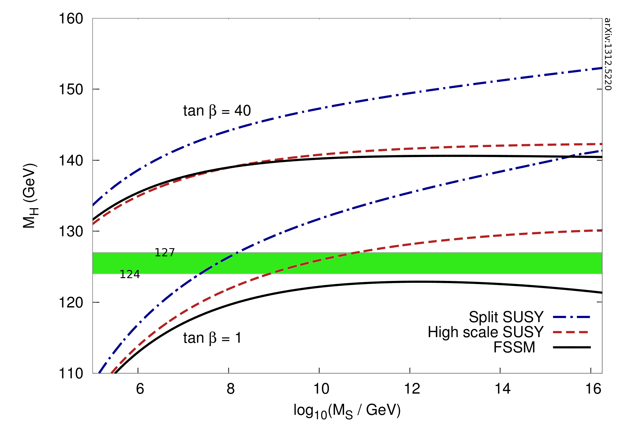
Figure 1: Higgs-mass predictions as a function of the SUSY scale $M_{\scriptscriptstyle S}$ for FSSM-I, High-Scale SUSY and Split SUSY. The green-shaded region indicates a Higgs mass in the range $[124,127]$ GeV.

Let us first describe how the Higgs mass is obtained in these models. The precise computations implies solving the RGEs through an iterative numerical algorithm which successively applies the boundary conditions at $M_{S}$ and at the electroweak scale. Schematically :

• We start by the determination of the values of gauge and Yukawa couplings at $M_{\scriptscriptstyle S}$ by evolving them from the experimental values at the electroweak scale to the SUSY scale.

• We determine the numerical value of $\lambda(M_{\scriptscriptstyle S})$ at the SUSY scale from its dependance on the gauge and Yukawa couplings. In the models under consideration $\lambda~{}=~{}\frac{1}{4}\left(g^{2}+g^{\prime\,2}\right)\,\cos^{2}2\beta+\Delta\lambda$, where $\Delta\lambda$ includes the threshold effects (suppressed in FSSM as discussed in [28])

• We run backwards in energies, use again the experimental values at the electroweak, and iterative the previous steps until convergence.

In order to understand the hurdles met when trying to reproduce the correct Higgs mass with an arbitrary high $M_{\scriptscriptstyle S}$, let us look at the way $\lambda$ evolves. The various contributions to $\beta_{\lambda}$ at one-loop can be roughly classified as:

$$\beta_{\lambda}=\frac{1}{16\pi^{2}} \left[\underbrace{12\lambda^{2}+\lambda(12y_{t}^{2}+(\cdots\tilde{g}^{2}\cdots)-(\cdots g^{2}\cdots))}_{\equiv~{}\beta_{\text{quartic}}}+\underbrace{(\cdots g^{4}\cdots)}_{\equiv~{}\beta_{g}}\underbrace{-(\cdots\tilde{g}^{4}\cdots)}_{\equiv~{}\beta_{\tilde{g}}}\underbrace{-12y_{t}^{4}}_{\equiv~{}\beta_{t}}\right]\ ,$$ (3.1)

where $(\cdots g^{n}\cdots)$ and $(\cdots\tilde{g}^{n}\cdots)$ contains contributions from contains gauge couplings and Higgs-higgsino-gaugino Yukawa couplings, respectively. Fixing $\lambda$ at $M_{\scriptscriptstyle S}$ and evolving it down to the electroweak scale, positive contributions tend to bring $\lambda$ towards lower values while negative contributions increases the Higgs mass. Two different effects explain the discrepancies between Split SUSY, High-Scale SUSY and FSSM:

1. Compared to Split SUSY, we see that both FSSM and High scale SUSY have vanishing $(\cdots\tilde{g}^{n}\cdots)$ terms. This decreases $\beta_{\lambda}(M_{\scriptscriptstyle S})$ in the Higgs scale SUSY and FSSM case.

2. High scale SUSY has smaller gauge couplings than FSSM and Split SUSY: these have extra fermions below $M_{\scriptscriptstyle S}$ which contribute in RGEs to push the couplings towards higher values.

These corrections are enhanced by a “domino” effect. At one-loop the top Yukawa coupling $y_{t}$ beta function $\beta_{t}$ has a positive contribution from $(\cdots\tilde{g}^{n}\cdots)$ terms and a negative one from $g_{3}$. Since $y_{t}$ is fixed at the electroweak scale, a smaller $\beta_{y_{t}}$ means a smaller $y_{t}$ at $M_{\scriptscriptstyle S}$. The split between different contributions to the $\beta$-functions is presented in Figure 2.

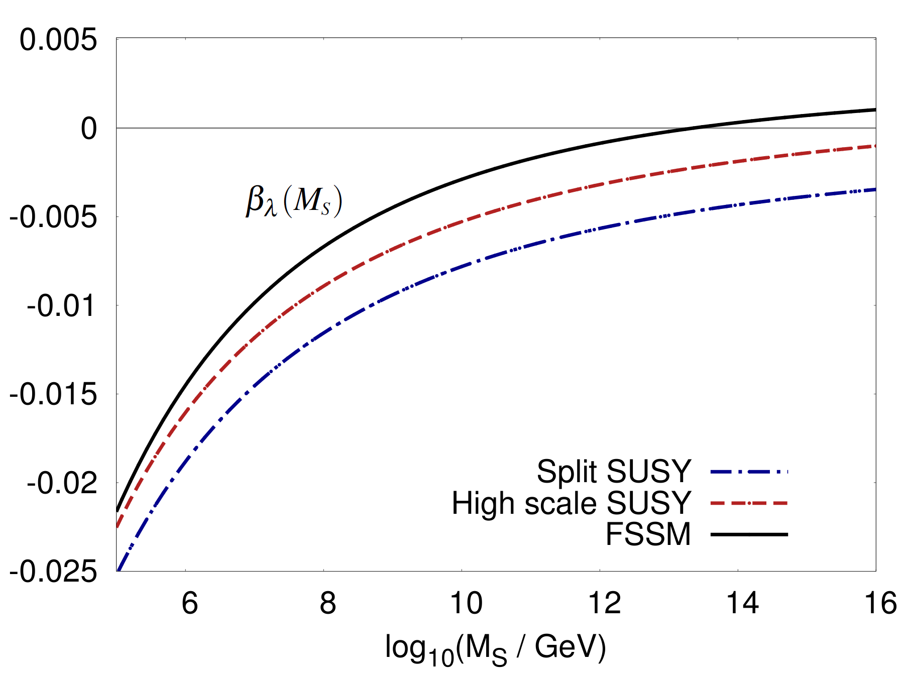
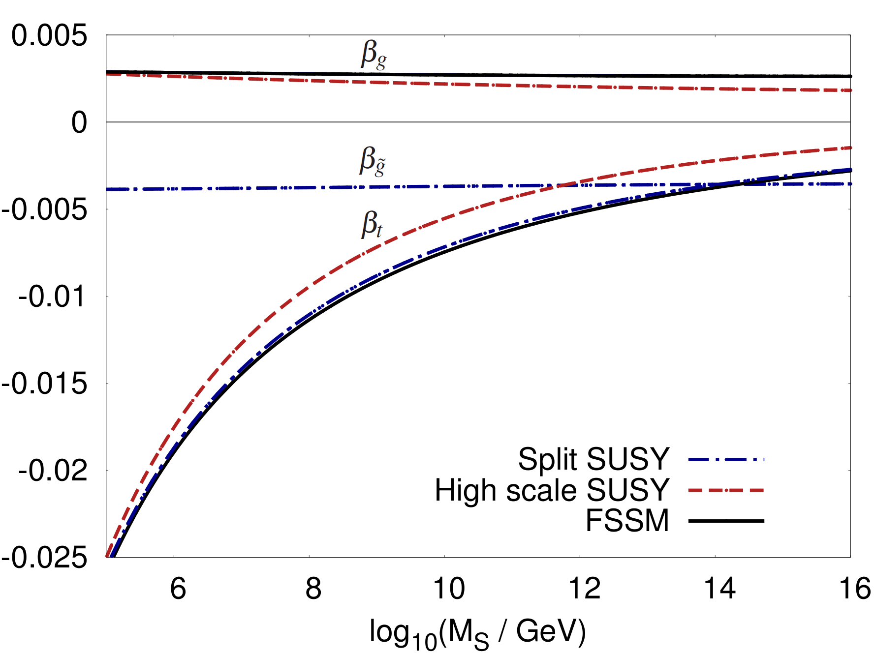
Figure 2: Left plot : $\beta_{\lambda}$ at $M_{\scriptscriptstyle S}$ for $\tan\beta=1$ in the case of Split SUSY, High scale SUSY and FSSM-I as a function of $M_{\scriptscriptstyle S}$. Right plot : Decomposition of $\beta_{\lambda}$ at $M_{\scriptscriptstyle S}$ into its various components $\beta_{t}$, $\beta_{g}$ (superposed for FSSM and Split SUSY) and $\beta_{\tilde{g}}$ as a function of $M_{\scriptscriptstyle S}$.

To summarise, the success of FSSM rests on simultaneously switching off the higgsinos Yukawa couplings while conserving stronger gauge couplings than High scale SUSY thanks to the presence of extra states at the TeV-scale. Similar arguments also explain why the Extended Split SUSY scenario presented in the Appendix of [29] predicts lower Higgs mass than the three scenarios described here. It keeps the suppression of $(\cdots\tilde{g}^{n}\cdots)$ terms while it enhances the gauge couplings.

3.2 Mega-Split vs Mini-Split

Another issue [31] in Split SUSY is that $M_{S}$ is further constrained to lower values when considering unified soft masses fro the Higgs field and tuning the Higgs mass at its measured value. This comes from the fact that RGEs for the Higgs sector soft masses does not preserve their quasi-degeneracy when running down from the unification scale. The longer the running above $M_{S}$, the higher the predicted $\tan\beta$, which leads to a higher Higgs mass at tree level. Hence it is natural to have larger values of $\tan\beta$ for small values of $M_{S}$, while for larger $M_{S}$ we can have $\tan\beta\sim 1$. A large value for $\tan\beta$ is not compatible with a 125 GeV Higgs mass with a large $M_{S}$ in the case of Split SUSY models [26, 27] thereof the ”Mini-Split”.

It is easy to see that low value of $\tan\beta$ are natural in FSSM, while this is not the case the Split SUSY models. At the SUSY scale, $\tan\beta$ is defined fixed by the requirement that one Higgs has a mass at the electroweak scale. In Split SUSY this fixes

$$\tan\beta~{}=~{}\sqrt{\frac{m_{H_{d}}^{2}+|\mu|^{2}}{m_{H_{u}}^{2}+|\mu|^{2}}}~{}\simeq~{}\sqrt{\frac{m_{H_{d}}^{2}}{m_{H_{u}}^{2}}}$$

since higgsinos are light. Renormalisation group evolution of $m_{H_{d}}^{2}$ and $m_{H_{u}}^{2}$, particularly due to the large top Yukawa coupling, then generates a $\tan\beta\gg\mathcal{O}(1)$. On the contrary, in FSSM, we have

$$\tan\beta~{}=~{}\sqrt{\frac{m_{H_{d}}^{2}+|\mu_{d}|^{2}}{m_{H_{u}}^{2}+|\mu_{u}|^{2}}}\ ,$$

with $\mu_{d}=\mu_{u}$ in the FSSM-I and $\mu_{u},\mu_{d}\simeq M_{\scriptscriptstyle S}$ since they are unrelated to the low energy spectrum. Note that the longer the running above $M_{S}$, the higher the predicted $\tan\beta$, which in turn raises the Higgs mass at tree level. Hence for small values of $M_{S}$ it is natural to have larger values of $\tan\beta$, and for larger $M_{S}$ we expect $\tan\beta\sim 1$.

In Figure 3 where we have plotted $\tan\beta$ in the FSSM-I as a function of unified SUSY-breaking scalar mass $m_{0}$ and the A-term at the GUT scale $A_{0}$. We see that in most of the parameter space $\tan\beta$ is between $1$ and $1.4$. The increase in the right part of the plot show that for a larger value of $A_{0}$, $m_{H_{u}}^{2}+\mu_{0}^{2}$ can run close to zero. In principle, by varying $m_{0}$ and $A_{0}$ in the FSSM-I we can find values of $\tan\beta>2$, potentially allowing values of the SUSY scale lower than $10^{9}$ GeV without requiring a breaking of the universality of the soft masses at the GUT scale.

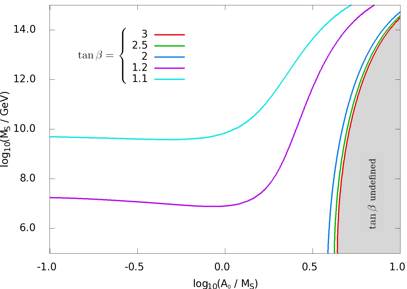
Figure 3: Contours of the value of $\tan\beta=\sqrt{\frac{m_{H_{d}}^{2}+|\mu_{d}|^{2}}{m_{H_{u}}^{2}+|\mu_{u}|^{2}}}$ in the FSSM-I varying the SUSY scale $M_{\scriptscriptstyle S}$ and the trilinear mass at $M_{\scriptscriptstyle S}$, $A_{0}$.

3.3 Constraints from cosmology

It is a standard result that gluinos are long-lived in SUSY models with heavy $M_{\scriptscriptstyle S}$. Since F-gluinos decay must proceed via mixing with the usual gluinos, their decay rates are even more suppressed. In [28, 29] we show that $\tau_{\tilde{g}^{\prime}}$, the F-gluino life-time is given by

$$\tau_{\tilde{g}^{\prime}}~{}\sim~{} 4\ \text{sec}\times\left(\frac{M_{S}}{10^{7}\text{GeV}}\right)^{6}\times\left(\frac{1\ \text{TeV}}{m_{fg}}\right)^{7}~{},$$ (3.2)

in the FSSM-I, where $m_{fg}$ is the F-gauginos mass scale. While in the FSSM-II, since the gauginos are not fake, this enhancement does not occur and one is left instead with the Split SUSY gluino life-time

$$\tau_{\tilde{g}^{\prime}}~{}\sim~{} 4\ \text{sec}\times\left(\frac{M_{S}}{10^{9}\text{GeV}}\right)^{4}\times\left(\frac{1\ \text{TeV}}{M_{1/2}}\right)^{5}~{},$$ (3.3)

where $M_{1/2}$ is the gauginos mass scale.

If one sticks with a standard cosmology the (F)-gluino lifetime is severely constrained, $\tau_{\tilde{g}}<100\text{s}$ [32]. Big-Bang Nucleosynthesis (BBN), the CMB spectrum and the gamma-ray background ruled out relic (F)-gluinos with lifetime between $10^{2}$ s until $10^{17}$ s. When the (F)-gluino is stable at the scale of the age of the universe, heavy-isotope searches also rule out such relic (F)-gluinos. This translates into limiting the SUSY scale to be below $5\cdot 10^{8}$ GeV for the FSSM-I and $5\cdot 10^{10}$ GeV for the FSSM-II. As it was underlined in [28], these constraints depends on wether or not one considers a “standard” cosmology. A late time reheating occuring before BBN could for instance dilute gluino relic. In such case, heavy-isotope searches are so stringent that they still constraint $\tau_{\tilde{g}}\lesssim 10^{16}\text{s}$ but one can avoid constraints from the CMB spectrum and the gamma-ray background, allowing therefore SUSY scales up to $10^{10}$ GeV for the FSSM-I and $10^{14}$ GeV for the FSSM-II.

It is however easy to find viable dark matter candidates in FSSM. We have distinguished three scenarios :

• Scenario $\tilde{H}|_{\text{DM}}$: F-higgsino LSP.

• Scenario $\tilde{W}|_{\text{DM}}$: (F-)Wino LSP.

• Scenario $\tilde{B}/\tilde{H}|_{\text{DM}}$: a mixed F-Bino/F-higgsino LSP, with a small splitting.

The relevant constraints are summarised in Table 3.3.

DM type	Inelastic scattering	Relic density	Gluino lifetime
$\mathbf{\tilde{W}|_{\text{DM}}}$	None	$m_{\tilde{W}}\subset[2390,2450]$ GeV	For multi-TeV gluinos $\begin{cases}M_{S}\lesssim 5\cdot 10^{8}\text{GeV}\\ \text{(for FSSM-I)}\\ \\ M_{S}\lesssim 2\cdot 10^{10}\text{GeV}\\ \text{(for FSSM-II)}\end{cases}$
$\mathbf{\tilde{B}/\tilde{H}|_{\text{DM}}}$	$\mu_{\text{pole}}\lesssim 900$ GeV	$m_{\tilde{B}}\simeq\mu_{\text{pole}}-(900-\mu_{\rm pole})/x_{f}$
$\mathbf{\tilde{H}|_{\text{DM}}}$	$\begin{cases}M_{S}\lesssim 5\cdot 10^{6}\text{GeV}\\ \text{(for FSSM-I)}\\ \\ M_{S}\lesssim 10^{8}\text{GeV}\\ \text{(for FSSM-II)}\end{cases}$	$\mu_{\text{pole}}\subset[1110,1140]$ GeV

Table 1: Approximate constraints on the SUSY scale and on pole masses for the Dark matter candidates. We impose a splitting between fake Higgsinos bigger than $300$ keV to avoid direct detection through inelastic scattering, we require a gluino life-time smaller than $100$ s to avoid hampering BBN and finally constrain the relic density (calculated at tree-level in micrOMEGAs) to be $\Omega h^{2}\subset[0.1158,0.1218]$. When considering constraints on $M_{S}$, gaugino masses were taken in the multi-TeV range.

The constraints on F-higgsinos dark matter (scenario $\mathbf{\tilde{H}|_{\text{DM}}}$ ) are in particular quite stringent. Indeed, since their couplings to the Higgs and (F)-gauginos are suppressed, the neutral higgsinos have a very small splitting. They are therefore a perfect example of inelastic dark matter and direct detection experiments constrain their mass splitting $\delta$ to be bigger than roughly $300$ keV [33, 34, 35]. Estimating the splitting by

$$\delta ~{}\simeq~{}\begin{cases}200\ \text{keV}\cdot\mathcal{O}(1)\cdot\displaystyle\left(\frac{400\text{ TeV}}{M_{\scriptscriptstyle S}}\right)^{2}\left(\frac{m_{fg}}{4\text{ TeV}}\right)\quad\textrm{ for the FSSM-I}\\ 200\ \text{keV}\cdot\mathcal{O}(1)\cdot\displaystyle\left(\frac{10^{7}\text{ GeV}}{M_{\scriptscriptstyle S}}\right)\left(\frac{\mu}{1\text{ TeV}}\right)\left(\frac{4\text{ TeV}}{m_{fg}}\right)\quad\textrm{ for the FSSM-II}\ ,\end{cases}$$ (3.4)

we recover the bounds from Table 3.3.

4 Conclusion

Two topics have been discussed here.

Clearly, if future LHC experiments find light new fermions that can be identified with signals of a Split-SUSY scenario, an experimental investigation of their precise quantum numbers and couplings will need to be determined. FSSM give a framework and further motivation for conducting such investigation.

The other topic discussed deals with the propagation of a spin-3/2 in a non-Lorentz invariant background (the fundamentals laws remaining Lorentz invariant). The Lagrangian was motivated by the study of the super-Higgs mechanism in a fluid, but can be taken and studied per se. It exhibits a feature common with spin-3/2 propagating in a curved space: the longitudinal modes ($\pm 1/2$ helicities) propagate at a slower speed, hence the “slow gravitino” name.

Acknowledgments

We would like to thank M. D. Goodsell, Y. Oz, G. Policastro and P. Slavich for collaborations on the different subjects presented here. This work is supported by the ERC advanced grant ERC Higgs@LHC, the ANR contract HIGGSAUTOMATOR and the Institut Lagrange de Paris.

References

- [1] K. Benakli, Y. Oz and G. Policastro, “The Super-Higgs Mechanism in Fluids,” JHEP 1402 (2014) 015 [arXiv:1310.5002 [hep-th]].
- [2] K. Benakli, L. Darmé and Y. Oz, “The Slow Gravitino,” JHEP 1410 (2014) 121 [arXiv:1407.8321 [hep-ph]].
- [3] R. Kallosh, L. Kofman, A. D. Linde and A. Van Proeyen, “Gravitino production after inflation,” Phys. Rev. D 61 (2000) 103503 [hep-th/9907124].
- [4] G. F. Giudice, I. Tkachev and A. Riotto, “Nonthermal production of dangerous relics in the early universe,” JHEP 9908 (1999) 009 [hep-ph/9907510].
- [5] G. F. Giudice, A. Riotto and I. Tkachev, “Thermal and nonthermal production of gravitinos in the early universe,” JHEP 9911 (1999) 036 [hep-ph/9911302].
- [6] A. Schenkel and C. F. Uhlemann, “Quantization of the massive gravitino on FRW spacetimes,” Phys. Rev. D 85 (2012) 024011 [arXiv:1109.2951 [hep-th]].
- [7] Y. Kahn, D. A. Roberts and J. Thaler, “The goldstone and goldstino of supersymmetric inflation,” JHEP 1510 (2015) 001 [arXiv:1504.05958 [hep-th]].
- [8] G. Velo and D. Zwanziger, “Propagation and quantization of Rarita-Schwinger waves in an external electromagnetic potential,” Phys. Rev. 186 (1969) 1337.
- [9] A. K. Das and M. Kaku, “Supersymmetry At High Temperatures,” Phys. Rev. D 18 (1978) 4540.
- [10] L. Girardello, M. T. Grisaru and P. Salomonson, “Temperature and Supersymmetry,” Nucl. Phys. B 178 (1981) 331.
- [11] K. Tesima, “Supersymmetry At Finite Temperatures,” Phys. Lett. B 123 (1983) 226.
- [12] D. Boyanovsky, “Supersymmetry Breaking at Finite Temperature: The Goldstone Fermion,” Phys. Rev. D 29 (1984) 743.
- [13] H. Aoyama and D. Boyanovsky, “Goldstone Fermions in Supersymmetric Theories at Finite Temperature,” Phys. Rev. D 30 (1984) 1356.
- [14] V. V. Lebedev and A. V. Smilga, “Supersymmetric Sound,” Nucl. Phys. B 318 (1989) 669.
- [15] R. G. Leigh and R. Rattazzi, “Supersymmetry, finite temperature and gravitino production in the early universe,” Phys. Lett. B 352, 20 (1995) [hep-ph/9503402];
- [16] K. Kratzert, “Finite temperature supersymmetry: The Wess-Zumino model,” Annals Phys. 308, 285 (2003) [hep-th/0303260];
- [17] “Supersymmetry breaking at finite temperature,” DESY-THESIS-2002-045;
- [18] P. Kovtun and L. G. Yaffe, “Hydrodynamic fluctuations, long time tails, and supersymmetry,” Phys. Rev. D 68, 025007 (2003) [hep-th/0303010].
- [19] C. Hoyos, B. Keren-Zur and Y. Oz, “Supersymmetric sound in fluids,” JHEP 1211, 152 (2012) [arXiv:1206.2958 [hep-ph]].
- [20] R. Jackiw, V. P. Nair, S. Y. Pi and A. P. Polychronakos, “Perfect fluid theory and its extensions,” J. Phys. A 37 (2004) R327 [hep-ph/0407101].
- [21] Z. Komargodski and N. Seiberg, “From Linear SUSY to Constrained Superfields,” JHEP 0909 (2009) 066 [arXiv:0907.2441 [hep-th]].
- [22] E. A. Bergshoeff, D. Z. Freedman, R. Kallosh and A. Van Proeyen, “Pure de Sitter Supergravity,” arXiv:1507.08264 [hep-th].
- [23] Nima Arkani-Hamed and Savas Dimopoulos. Supersymmetric unification without low energy supersymmetry and signatures for fine-tuning at the LHC. JHEP, 06:073, 2005.
- [24] G. F. Giudice and A. Romanino. Split supersymmetry. Nucl. Phys., B699:65–89, 2004. [Erratum: Nucl. Phys.B706,65(2005)].
- [25] N. Arkani-Hamed, S. Dimopoulos, G. F. Giudice, and A. Romanino. Aspects of split supersymmetry. Nucl. Phys., B709:3–46, 2005.
- [26] Nicolás Bernal, Abdelhak Djouadi, and Pietro Slavich. The MSSM with heavy scalars. Journal of High Energy Physics, 2007(07):016, 2007.
- [27] Gian F. Giudice and Alessandro Strumia. Probing High-Scale and Split Supersymmetry with Higgs Mass Measurements. Nucl. Phys., B858:63–83, 2012.
- [28] Karim Benakli, Luc Darmé, Mark D. Goodsell, and Pietro Slavich. A Fake Split Supersymmetry Model for the 126 GeV Higgs. JHEP, 1405:113, 2014.
- [29] K. Benakli, L. Darmé and M. D. Goodsell, “(O)Mega Split,” arXiv:1508.02534 [hep-ph].
- [30] Emilian Dudas, Mark Goodsell, Lucien Heurtier, and Pantelis Tziveloglou. Flavour models with Dirac and fake gluinos. Nucl. Phys., B884:632–671,
- [31] A. Arvanitaki, N. Craig, S. Dimopoulos and G. Villadoro, “Mini-Split,” JHEP 1302 (2013) 126 [arXiv:1210.0555 [hep-ph]].
- [32] Asimina Arvanitaki, Chad Davis, Peter W. Graham, Aaron Pierce, and Jay G. Wacker. Limits on split supersymmetry from gluino cosmology. Physical Review D, 72(7):075011, 2005.
- [33] Natsumi Nagata and Satoshi Shirai. Higgsino Dark Matter in High-Scale Supersymmetry. JHEP, 1501:029, January 2015.
- [34] XENON collaboration. Implications on Inelastic Dark Matter from 100 Live Days of XENON100 Data. Phys.Rev., D84:061101, 2011.
- [35] LUX collaboration. First results from the LUX dark matter experiment at the Sanford Underground Research Facility. Phys.Rev.Lett., 112:091303, March 2014.