Polymer models with competing collapse interactions on Husimi and Bethe lattices

Abstract

In the framework of Husimi and Bethe lattices, we investigate a generalized polymer model that incorporates as special cases different models previously studied in the literature, namely, the standard interacting self-avoiding walk, the interacting self-avoiding trail, and the vertex-interacting self-avoiding walk. These models are characterized by different microscopic interactions, giving rise, in the two-dimensional case, to collapse transitions of an apparently different nature. We expect that our results, even though of a mean-field type, could provide some useful information to elucidate the role of such different theta points in the polymer phase diagram. These issues are at the core of a long-standing unresolved debate.

I Introduction

The collapse transition of a polymer chain in dilute solution is one of the most classical topics in polymer physics de Gennes (1979); des Cloizeaux and Jannink (1990); Vanderzande (1998). Such a phenomenon arises from a competition between excluded volume and some kind of attractive interaction of the monomers with one another. Depending on which of the two effects prevails, the polymer takes on a swollen state (coil) or a compact one (globule), also denoted as good- or bad-solvent regimes, respectively. The two regimes are separated by a phase transition (driven by temperature, or by some actual change in the solvent quality), which is characterized by specific properties of the polymer, usually denoted as the theta state.

Different lattice models have been proposed to investigate these phenomena. In the standard interacting self-avoiding walk (ISAW) model de Gennes (1979); des Cloizeaux and Jannink (1990); Vanderzande (1998), polymers are forbidden from visiting a lattice site more than once, and a contact interaction is assigned to nearest-neighbor sites visited by nonconsecutive monomers. Alternative models are the interacting self-avoiding trail (ISAT) Massih and Moore (1975); Foster (2009) and the vertex-interacting self-avoiding walk (VISAW) Blöte and Nienhuis (1989); Foster and Pinettes (2003), both characterized by the fact that only lattice bonds (not sites) are subject to the single-visit constraint. The two models differ in the fact that the ISAT is allowed to cross itself, whilst the VISAW is not. In both cases, the self-attractive interaction is associated with the multiply-visited sites.

According to the paradigm of universality, one would expect that the critical behavior of all three of the above models should be described by the same universality class. Indeed, this seems to be the case in the good-solvent regime (which is itself a critical state), but there are several evidences that, in two dimensions, the theta state belongs to three different universality classes and, for the ISAT and VISAW cases, it is also associated to the onset of a peculiar maximally-dense phase Foster and Pinettes (2003); Foster (2009); Bedini et al. (2013a) and other more subtle features Nahum et al. (2013); Vernier et al. (2015). Note that two-dimensional models have attracted great theoretical interest, due to the availability of rigorous results coming from exact solutions and/or conformal field theories, through the analogy with “magnetic” $O(n)$ models in the limit ${n\to 0}$ de Gennes (1979); des Cloizeaux and Jannink (1990); Vanderzande (1998). The ISAW theta point has been clearly identified as a tricritical point in the language of $O(n)$ models, and all of its properties are quite well-established, with good agreement between theory Duplantier and Saleur (1987) and simulations Caracciolo et al. (2011) for the values of critical exponents. Conversely, a number of contradictory results have emerged for the ISAT and VISAW theta points, in particular some striking discrepancies among Monte Carlo simulations Meirovitch and Lim (1988); Owczarek and Prellberg (2007); Bedini et al. (2013a, b), numerical transfer-matrix methods Blöte and Nienhuis (1989); Foster and Pinettes (2003); Foster (2009, 2011); Foster and Pinettes (2012), field-theoretic arguments Jacobsen et al. (2003); Nahum et al. (2013); Vernier et al. (2015), and exact results Warnaar et al. (1992).

In this article, we study a generalized polymer model that incorporates all the aforementioned ones, in the framework of Husimi Pretti (2002); Serra et al. (2004); Zara and Pretti (2007); Oliveira et al. (2008); Neto and Stilck (2013) and Bethe lattices Lise et al. (1998); Buzano and Pretti (2002); Pretti (2006); Serra and Stilck (2007); Neto and Stilck (2008). The free parameters characterizing such lattices (building blocks, coordination numbers) are chosen, according to experience, in order to obtain the best possible approximation to a regular 2d square lattice model. The motivation for this work stems from the difficulty of extracting, from the existing literature, a unified view of the phase diagram in the presence of the different topological constraints and competing collapse interactions described above. Indeed, considerable work has been done in this direction in particular by Bedini, Owczarek, and Prellberg (making use of refined Monte Carlo simulations) Bedini et al. (2013a, c, 2014) and by Foster and Pinettes (mainly by means of numerical transfer-matrix techniques) Foster and Pinettes (2003); Foster (2009, 2011); Foster and Pinettes (2012), but several unresolved issues and contradictory results still remains. Just to give a couple of examples, the mentioned authors have investigated an asymmetric ISAT (denoted as AISAT) on the square lattice, where doubly-visited sites with or without crossing are assigned a different attractive interaction. Now, in the special case of crossing interactions only, the transfer-matrix results Foster (2011) suggest the onset of a first-order collapse, while the simulations Bedini et al. (2013a) seem to predict a revival of the ISAW theta state, i.e., a weak continuous transition, with no evidence of a maximally-dense phase. Moreover, whilst an exact solution Warnaar et al. (1992) of the VISAW model predicts a correlation-length exponent ${\nu=12/23}$, Monte Carlo simulations Bedini et al. (2013b) suggest the ISAW value ${\nu=4/7}$, and transfer-matrix methods Blöte and Nienhuis (1989); Foster and Pinettes (2012) are incompatible with both results.

In this context, a clear advantage of the approach developed in the current article is the possibility of a sharp determination of the phase diagram (with extremely high numerical precision in the case of the Husimi lattice, even analytical in the case of the Bethe lattice). For instance, we have no ambiguity on the order of the transitions, which is usually not the case with methods affected by higher numerical uncertainties. On the other hand, a primary drawback of the matter is that the resulting phase diagram, indeed exact on such infinite-dimensional treelike lattices, is not guaranteed to correspond to the actual phase diagram of the 2d model. Concerning this point, we have nonetheless to say that Husimi and Bethe lattice models often turn out to exhibit a remarkably good qualitative agreement with finite-dimension results, when the latter are well-established by other methods. This has been observed in different polymer models, such as the semiflexible ISAW Pretti (2002); Lise et al. (1998); Bastolla and Grassberger (1997) or the bond-ISAW Buzano and Pretti (2002); Foster and Seno (2001); Foster (2007), and holds true, as we shall see, at least in a limiting case of the model under investigation Bedini et al. (2013c, 2014). Indeed, we shall see that the Bethe lattice model yields a slightly less convincing behavior for the general case, but we have found it interesting (and therefore we have included it in the article), mostly by virtue of the opportunity of a fully analytical solution.

A more substantial difficulty of our approach is that, even though the Husimi or Bethe solutions take into account certain local correlations, they still have a mean-field nature, so that in principle they cannot predict critical exponents. As a consequence, the universal points are to be naively identified on the basis of physical intuition, and/or according to their role in the phase diagram. In conclusion, we cannot expect that our results provide definitive answers to the open problems of the 2d case, in particular to the issue of universality classes, but we believe they might be nonetheless of some use, mainly as a coherent set of hypotheses, yet to be tested by more specific methods.

The paper is organized as follows. In Sec. II we give a precise definition of the model that we are going to investigate. In Sec. III we briefly present the Husimi lattice solution, whose details are reported separately in Appendix A. Sec. IV contains all the results concerning the Husimi lattice model, whereas Sec. V is devoted to a discussion and some concluding remarks. The Bethe lattice solution is reported in full detail in Appendix B, along with a comparison with the Husimi lattice one.

II The model

Let us define the model on the regular two-dimensional square lattice, as in the original (partial) versions. The definition for the Husimi or Bethe lattices follows in a straightforward way. The polymer is represented as a self-avoiding trail, that is, a walk such that lattice bonds can be visited only once, whereas lattice sites can be visited more than once (at most twice on the square lattice). Doubly-visited sites are assigned a Boltzmann weight $\tau_{\mathrm{x}}$ or $\tau_{\mathrm{c}}$, depending on whether the walk self-intersects or not, respectively. Moreover, a weight $\omega$ is assigned to every pair of nearest-neighbor sites, that are visited (once) by nonconsecutive monomers. The latter type of statistical weight is the usual one for the ISAW. All kinds of weights are summarized in Fig. 1. For simplicity, in the following we shall denote the configurations weighted by $\omega$ as contacts, whereas those weighted by $\tau_{\mathrm{c}}$ and $\tau_{\mathrm{x}}$ will be denoted as collisions and crossings.

Figure 1: An example of polymer configuration on the 2d square lattice, along with the statistical weights associated to the different interactions: $\omega$ is associated to nearest-neighbor sites visited (once) by nonconsecutive monomers; $\tau_{\mathrm{c}}$ and $\tau_{\mathrm{x}}$ are associated to doubly-visited sites with, respectively, colliding or crossing configurations.

Let us briefly explain how this model incorporates different polymer models, that have been previously studied in the literature. First of all, when ${\tau_{\mathrm{x}}=\tau_{\mathrm{c}}\equiv\tau}$ (i.e., collisions and crossings are equally weighted), we obtain the Wu-Bradley model Wu and Bradley (1990), which has recently been the subject of an accurate numerical investigation by Bedini and coworkers Bedini et al. (2014). In turn, the latter model contains the ordinary ISAT model for ${\omega=1}$ (i.e., without contact interactions), the ordinary ISAW model for ${\tau=0}$ (i.e., forbidding doubly-visited sites), and also the so-called interacting nearest-neighbor self-avoiding trail (INNSAT) model Bedini et al. (2013c) for ${\tau=1}$ (i.e., a self-avoiding trail with contact interactions only). The latter model has been proposed in the cited article, in order to investigate the stability of the ISAW theta state with respect to a change in the self-avoidance contraints. Furthermore, for ${\omega=1}$ and ${\tau_{\mathrm{x}}\neq\tau_{\mathrm{c}}}$, we obtain the previously mentioned AISAT model Foster (2011); Bedini et al. (2013a), studied in order to test the stability of the ISAT theta state with respect to perturbations in the attractive interaction. The latter model contains in turn the VISAW model, in the limiting case ${\tau_{\mathrm{x}}=0}$ (crossings forbidden).

We shall consider the model in a grand-canonical description, with a fugacity parameter $\zeta$ associated to each polymer segment, that is, to each visited bond. The partition function can thus be written as

$$\Xi=\sum_{\mathrm{SAT}}\omega^{\mathcal{N}_{\mathrm{n}}}\tau_{\mathrm{c}}^{\mathcal{N}_{\mathrm{c}}}\tau_{\mathrm{x}}^{\mathcal{N}_{\mathrm{x}}}\zeta^{\mathcal{N}_{\mathrm{s}}}$$ (1)

where $\mathcal{N}_{\mathrm{s}}$ denotes the number of visited bonds, and $\mathcal{N}_{\mathrm{n,c,x}}$ denote respectively the number of contacts, collisions, and crossings. The sum is understood to run over all configurations compatible with the self-avoiding trail constraint. Note that, since we are interested in the properties of infinitely long polymers, this set of configurations does not include loops whose length remains finite in the thermodynamic limit.

III The Husimi lattice solution

Figure 2: Sketch of a Husimi lattice made up of square clusters.

A Husimi tree is a self-similar lattice like the one depicted in Fig. 2, where it is understood that the size of the tree is arbitrarily increased (toward a thermodynamic limit) by a self-replicating growth procedure. In a wide part of the literature, a Husimi lattice is defined as the “inner region” of a corresponding infinite Husimi tree Lavis and Bell (1999), meaning a region where a homogeneity condition holds for thermal averages of local observables (for instance, the site magnetization for the ferromagnetic Ising model). Such thermal averages can thus be determined by the fixed points of relatively simple self-consistency equations. Unfortunately, due to the fact that in a Husimi tree the majority of sites is located on the boundary, it turns out that in certain cases boundary conditions heavily affect the properties of the inner region as well, which is not a good fact to the purpose of approximating the thermodynamic behavior of a regular lattice model. For a discussion of these issues, see for instance Refs. Pretti, 2003; Ostilli, 2012. The Husimi lattice is therefore better defined Dorogovtsev et al. (2008) as an ensemble of random-regular hyper-graphs, that are, roughly speaking, random graphs made up of a unique type of hyper-edge (for instance, a square cluster as in Fig. 2), with a fixed coordination number. This kind of systems have no boundary, so that the problem of boundary conditions is avoided, and are locally treelike, since the length of closed paths diverges as the logarithm of the number of sites in the thermodynamic limit (excluding of course short paths that are closed within single clusters). The latter fact means that a Husimi lattice still looks (locally) like Fig. 2 and, more importantly, that its thermodynamic properties can still be derived in terms of simple self-consistency equations. Of course, our choice to use square clusters as building blocks, and a coordination number $2$ (in this context, we define the coordination number as the number of building blocks attached to each given site) is motivated by the purpose of approximating the model on the ordinary 2d square lattice. The self-consistency equations (a.k.a. recursion equations) can be worked out in different ways. A possible way, which we believe likely to be the simplest one, is to derive them as stationarity conditions for a suitable variational free energy density.

Let us consider the grand-canonical free-energy density per site (in $k_{\mathrm{B}}T$ units)

$$\psi=-\lim_{N\to\infty}\frac{1}{N}\ln\Xi\,,$$ (2)

where $N$ denotes the number of sites. For the Husimi lattice defined above, this free-energy density can be written as

$$\psi=-\frac{1}{2}\ln q+\ln z\,,$$ (3)

where $q$ is the cluster partition function, $z$ is the single-site partition function, and $1/2$ is the ratio between the number of square clusters and the number of sites present in the system. Roughly speaking, the single-site term may be regarded as a correction over the cluster term, due to the overlap between clusters.

The cluster partition function $q$ is the partition function of a small subsystem made up of four sites on a square cluster, interacting with one another and with effective fields that represent the remainder of the system. It will therefore take the following form

$$q=\sum_{i,j,k,l}\chi_{i,j,k,l}w_{i}w_{j}w_{k}w_{l}\,,$$ (4)

where $i,j,k,l$ are labels for the polymer configurations on each site, $\chi_{i,j,k,l}$ is the statistical weight of interactions inside the square cluster (including topological constraints), and $w_{i}$ are the effective fields. Note that these fields are sometimes called cavity fields, since they represent the probabilities of site configurations for a system in which a cluster interaction is removed (that is, replaced by a cavity). Moreover, ${-\ln q}$ can be regarded as the free-energy shift between the system with a cavity and the unperturbed system. For clarity, let us note that, in most papers dealing with polymer models on Husimi or Bethe lattices, the cavity fields are called partial partition functions. In equation (4) the treelike nature of the system is reflected in the fact that, in the absence of the cluster interaction, the joint probability distribution factorizes, meaning that the site configurations are statistically independent. Indeed, in a real tree-graph the removal of a cluster splits the system into noninteracting subsystems (usually called branches).

The single-site partition function $z$ is a similar quantity for a single site, interacting with two cavity fields associated to the two “branches” attached to the given site. It can be written in the following form

$$z=\sum_{i,j}\chi_{i,j}w_{i}w_{j}\,.$$ (5)

Note that we have two configuration labels $i,j$ even though for a single site, because it is convenient to define the local polymer configurations with respect to two different reference frames, integral with each branch. As a consequence, the same configuration may be identified by different labels with respect to different branches. Moreover, the statistical weight $\chi_{i,j}$ also has to ensure consistency between the two labels. This issue should get clearer in Appendix A, where we report the explicit expression of $z$.

All the information needed to solve the model is contained in equations (3), (4), and (5), provided explicit expressions of the statistical weights $\chi_{i,j,k,l}$ and $\chi_{i,j}$ (and therefore of $q$ and $z$) are derived. As previously mentioned, equilibrium states are determined by the stationarity conditions for the free energy, namely,

$$\frac{\partial\psi}{\partial w_{i}}=0\,,$$ (6)

which can be easily written in a self-consistent form

$$w_{i}\propto f_{i}(w_{0},w_{1},w_{2},w_{3})\,.$$ (7)

Explicit expressions for the functions $f_{i}$ are also reported in Appendix A, along with a proof that 4 cavity fields (denoted as ${w_{0},\dots,w_{3}}$) suffice to represent all the relevant configurations. The recursion equations (7) can be solved numerically by a simple iterative algorithm. Note that a proportionality constant remains undetermined, because the free-energy density $\psi$ is invariant under multiplication of each cavity field by a constant, as one can easily verify. As usual, we fix the constant so as to satisfy, at each iteration, a normalization condition, namely

$$\sum_{i=0}^{3}w_{i}=1\,.$$ (8)

For the benefit of readers who are not familiar with Husimi lattice models, let us briefly note that the self-consistent form is not only an efficient way to solve numerically a set of nonlinear simultaneous equations, but it can be interpreted as a self-similarity condition, namely, the equality between the cavity fields associated to a given branch and those of its sub-branches. Indeed, most studies directly derive the recursion equations via self-similarity.

All equilibrium properties of the system can now be derived from the knowledge of the cavity field values satisfying equations (7), along with the expression of the free-energy density, equations (3), (4), and (5). The average number of segments per site, which in the following we shall briefly refer to as segment density, or simply density, can be evaluated as

$$\rho=-\frac{\partial\psi}{\partial\ln\zeta}\,.$$ (9)

Note that, in the above derivative, the dependence on $\zeta$ of the cavity fields can be neglected, because we are interested in equilibrium points, and the derivatives of $\psi$ with respect to the cavity fields vanish at such points. The density $\rho$ is the main order parameter for our system. Other meaningful observables are the average number of contacts per site (contact density)

$$\eta=-\frac{\partial\psi}{\partial\ln\omega}$$ (10)

and the average number of collisions or crossings per site (respectively, collision or crossing density)

$$\xi_{\mathrm{c,x}}=-\frac{\partial\psi}{\partial\ln\tau_{\mathrm{c,x}}}\,.$$ (11)

Explicit expressions for $\xi_{\mathrm{c}}$, $\xi_{\mathrm{x}}$, and $\eta$ can be derived straightforwardly.

In the presence of multiple solutions (i.e., fixed points) of the recursion equations, revealing the occurrence of coexistence phenomena, the free-energy values allow one to discriminate the thermodynamically stable phase, and therefore to determine first-order transitions. Conversely, second-order transitions can be better detected by analyzing the stability of the solutions. The latter is a rather technical issue, which we discuss in Appendix A.

IV Results

In the framework of the grand-canonical formulation, the phase diagram can be described as a function of the Boltzmann weights of the elementary interactions, also denoted as activities (in our case $\tau_{\mathrm{c}}$, $\tau_{\mathrm{x}}$, and $\omega$), and of the fugacity variable $\zeta$, which controls the segment density. For given activity values, we expect a phase transition to occur at a certain fugacity $\zeta_{0}(\tau_{\mathrm{c}},\tau_{\mathrm{x}},\omega)$, where the density changes from ${\rho=0}$ for ${\zeta<\zeta_{0}}$ to ${\rho>0}$ for ${\zeta>\zeta_{0}}$. The transition manifold, defined by the function $\zeta_{0}$, can be identified as the canonical thermodynamic limit for a single polymer chain, and in particular ${\ln\zeta_{0}}$ represents the corresponding Helmholtz free-energy density per segment (in ${k_{\mathrm{B}}T}$ units). In the limit ${\zeta\to\zeta_{0}^{+}}$, the properties of the dense phase are expected to approach those of a single chain (we shall denote it as the “single-chain” limit), so that, in particular, the segment density $\rho$ can be viewed as a measure of the chain compactness. Therefore, a second-order transition represents a swollen state, whereas a first-order transition represents a collapsed state. For the well-known ISAW model (${\tau_{\mathrm{x}}=\tau_{\mathrm{c}}=0}$ in our scheme), increasing the contact activity $\omega$ (which usually means lowering the temperature) drives the system from the former to the latter regime, giving rise to a continuous transition (theta collapse).

Solving the recursion equations (7), we find, besides the zero-density phase (also denoted as 0 phase in the following), two different dense phases: an “ordinary” one (1 phase), and a “maximally dense” one (2 phase). The 2 phase is characterized by very large values of the segment density $\rho$ and of the crossing-collision density ${\xi\equiv\xi_{\mathrm{c}}+\xi_{\mathrm{x}}}$ (quite close to the respective upper bounds ${\rho=2}$ and ${\xi=1}$), and by small values of the contact density $\eta$ (quite close to $0$). Conversely, the 1 phase is characterized by smaller values of $\rho$ and $\xi$, and larger values of $\eta$. The segment density $\rho$ is the natural order parameter for both 0-1 and 0-2 phase transitions, because the 0 phase is characterized by ${\rho=0}$, whereas ${\rho>0}$ in the 1 and 2 phases. The 1-2 transition cannot be defined rigorously in terms of densities, but a suitable order parameter is instead the $w_{1}$ cavity field, which turns out to be strictly positive in the 1 phase and zero in the 2 phase.

IV.1 Wu-Bradley model

Let us first analyze the case of a symmetric crossing-collision interaction (${\tau_{\mathrm{x}}=\tau_{\mathrm{c}}\equiv\tau}$), which has been previously denoted as the Wu-Bradley model. We shall present a sequence of projections of the grand-canonical phase diagram in the plane $\zeta$ vs $\tau$, for different fixed values of the contact activity, namely, ${\omega=1.2,0.5,1}$. Note that ${\omega>1}$ or ${\omega<1}$ means that contacts are energetically favored or disfavored, respectively, whereas the case ${\omega=1}$ corresponds to the ISAT model, with no contact interaction.

The phase diagram for ${\omega=1.2}$ is displayed in Fig. 3.

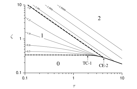
Figure 3: Grand-canonical phase diagram ($\zeta$ vs $\tau$) for ${\omega=1.2}$. The zero-density phase, the ordinary dense phase, and the maximally-dense phase are denoted respectively by 0, 1, 2. Solid lines denote first order transitions; dashed lines denote second order transitions. Thin solid lines are contour lines of the segment density per site (numerals denoting density values). The point at which the 0-1 transition changes from second to first order is tagged as TC-1. The critical end-point, terminating the (second-order) 1-2 transition line, is tagged as CE-2.

The transition line between the 0 and 1 phases turns out to be partially first and partially second order. The point separating the two regimes represents a continuous collapse in the single-chain limit, so that it can be viewed as the analogous of the theta point of the ISAW model, which is, a tricritical point in the language of $O(n)$ models. We shall denote this point as TC-1 to avoid misunderstandings, because, as previously mentioned, the theta point of the ISAW model corresponds to a well-defined universality class, whereas Husimi lattice models necessarily belong to a mean-field universality class. In the dense region (${\rho>0}$) a second-order transition line separates the 1 and 2 phases. This line joins to the transition line with the 0 phase at a critical end-point, which we shall denote as CE-2. The latter corresponds, in the single-chain limit, to a continuous transition between two different regimes of the collapsed state. The regime associated to the first-order portion of the 0-1 phase represents a moderately compact state, whose density rapidly increases upon increasing $\tau$. On the other hand, the regime associated to the 0-2 transition (which is all first-order) represents a very compact state, with a large majority of doubly-visited sites, whose density value is almost saturated around ${\rho\lesssim 2}$. These observations can be confirmed by inspection of the density contour lines, reported in Fig. 3.

The transition scenario changes considerably for ${\omega<1}$. Fig. 4 displays the $\zeta$ vs $\tau$ phase diagram in the particular case ${\omega=0.5}$.

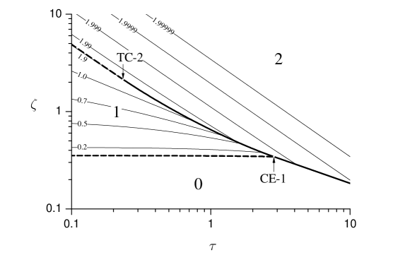
Figure 4: Grand-canonical phase diagram ($\zeta$ vs $\tau$) for ${\omega=0.5}$. Lines and phase tags are as in the previous figure. The critical end-point, that terminates the (second-order) 0-1 transition line, is tagged as CE-1. The point at which the 1-2 transition changes from second to first order is tagged as TC-2.

The TC-1 point disappears, so that the 0-1 transition line is now all second-order. Conversely, the 1-2 transition line turns out to be partially second and partially first order. As a consequence, the 0-1 transition line terminates in a critical end-point, which we denote as CE-1. The latter also marks the separation between the first-order portion of the 1-2 transition line and the (all first order) 0-2 transition line. In the single-chain limit the CE-1 point represents a discontinuous (first order) collapse transition to the very compact state with almost saturated density.

Analyzing the evolution of the $\zeta$ vs $\tau$ phase diagram between the two regimes observed, from ${\omega=1.2}$ to ${\omega=0.5}$, we realize that all the relevant changes occur precisely at ${\omega=1}$, that is, in the case of the pure ISAT model. The phase diagram for this case is reported in Fig. 5.

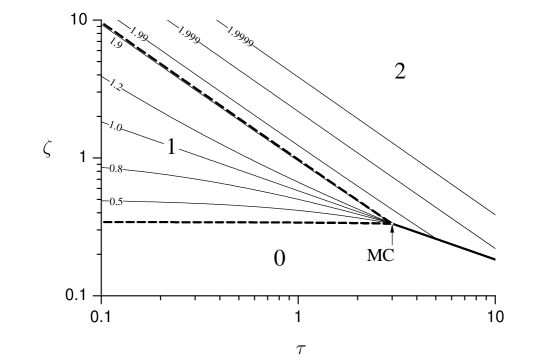
Figure 5: Grand-canonical phase diagram ($\zeta$ vs $\tau$) for ${\omega=1}$ (ISAT model). Lines and phase tags are as in the previous figures. The multicritical point is tagged as MC.

We can observe that all four of the “special points” defined above, namely, TC-1, TC-2, CE-1, and CE-2 degenerate into a unique multicritical point (tagged as MC). In the single-chain limit, this point still represents an abrupt collapse transition to the saturated compact state, but it turns out to exhibit rather peculiar features. First of all, it is located precisely at ${\tau=3}$ and ${\zeta=1/3}$. These values, which we can determine with very high numerical precision (of the order of ten decimal places), coincide with those pointed out (though with lower precision) by both simulations Bedini et al. (2014) and transfer-matrix techniques Foster (2009). Furthermore, we can observe that all the density contour lines in the 1 phase converge toward the MC point. This means that precisely at the MC point there exists a continuum of solutions of the recursion equations (i.e., a continuum of minima of the free energy), all with the same free-energy value, but with densities ranging from zero (the 0-phase value) up to the 2-phase value. In other words, we can state that the 0 phase and the 2 phase remain distinct, but the free energy barrier associated with the 0-2 (first-order) transition vanishes precisely at the MC point. As far as the single-chain limit is concerned, we might analogously say that the collapse transition of the ISAT model is a discontinuous transition with a zero free-energy barrier. Finally, it is noticeable that both the location and the specific features of the MC point are preserved even in the Bethe lattice solution. In this case all the details reported above can be probed analytically, as discussed in Appendix B. In particular, it turns out that, in a Landau expansion of the variational free energy, the derivatives of any order vanish precisely at the MC point. This is just the mean-field representation of a multicritical point of infinite order, which remarkably agrees with the characterization of the ISAT theta point, recently given by Nahum and coworkers. Nahum et al. (2013)

To complete the picture of the phase diagram for the Wu-Bradley model, we have systematically analyzed the evolution of the “special points” as a function of $\omega$. This analysis leads to the graph reported in Fig. 6, which can also be regarded as a single-chain phase diagram.

Figure 6: Single-chain phase diagram ($\tau$ vs $\omega$). Here 0, 1, and 2 denote respectively the swollen state, the moderately-compact and the highly-compact states. The solid line and the dashed line represent the evolution of the CE-1 and CE-2 points, respectively. The evolution of the TC-1 and TC-2 points is represented by the dash-dotted and dotted lines, respectively. Note that TC-2 points lie outside the 0-phase boundary, and do not represent single-chain transitions.

Indeed, all the special points, except TC-2, lie on the ${\zeta=\zeta_{0}}$ manifold (i.e., on the 0-phase boundary), and represent certain conformational transitions for a single polymer chain in the thermodynamic limit (note that all the points except MC evolve into lines upon varying $\omega$). In particular: TC-1 represents a continuous ISAW-like collapse from a swollen state to a moderately compact state, CE-2 represents another continuous collapse from the moderately compact to the highly compact or saturated state; CE-1 represents a direct discontinuous (first-order) collapse from the swollen state to the highly compact state. Finally, MC can be regarded as a limiting case of CE-1, in which the free-energy barrier vanishes.

IV.2 Generalized model and AISAT model

Let us now switch to the general case ${\tau_{\mathrm{x}}\neq\tau_{\mathrm{c}}}$. Let us note that, in principle, a complete description of the phase diagram would require the exploration of the whole four-parameters space ($\zeta,\omega,\tau_{\mathrm{c}},\tau_{\mathrm{x}}$), which would be a rather heavy task. Nevertheless, it turns out that the description can be considerably simplified by introducing suitable alternative parameters, namely, a particular average crossing-collision activity

$$\tau\equiv\frac{2\tau_{\mathrm{c}}+\tau_{\mathrm{x}}}{3}\,,$$ (12)

and an asymmetry parameter

$$\Gamma\equiv\frac{\tau_{\mathrm{x}}-\tau_{\mathrm{c}}}{\tau_{\mathrm{x}}+\tau_{\mathrm{c}}}\,.$$ (13)

The range of the latter turns out to be the interval $[-1,1]$, where ${\Gamma=0}$ corresponds to the symmetric case ${\tau_{\mathrm{x}}=\tau_{\mathrm{c}}=\tau}$ (Wu-Bradley model), whereas ${\Gamma=+1,-1}$ correspond respectively to the extreme asymmetric cases ${\tau_{\mathrm{c}}=0}$ and ${\tau_{\mathrm{x}}=0}$ (VISAW model).

The key-point is that, for fixed $\Gamma$ values, the single-chain phase diagram in the $\tau$ vs $\omega$ plane remains topologically equivalent to that of the symmetric case (Fig. 6), with just a small displacement of the MC-point location $(\omega_{\mathrm{MC}},\tau_{\mathrm{MC}})$ with respect to its “original” position $(1,3)$. A parametric plot of $(\omega_{\mathrm{MC}},\tau_{\mathrm{MC}})$ as a function of $\Gamma$ is reported in Fig. 7.

Figure 7: Parametric plot of the position of the MC point in the $\tau$ vs $\omega$ plane, as a function of $\Gamma$. Special $\Gamma$ values are indicated by arrows.

We notice a peculiar cusp around the point $(1,3)$, which can be characterized as follows. We verify numerically that for small $\Gamma$, the MC-point coordinates behave as

$$\tau_{\mathrm{MC}}-3 \sim \Gamma^{2}\,,$$ (14)

$$\omega_{\mathrm{MC}}-1 \sim \Gamma^{3}\,.$$ (15)

This obviously imply

$$\tau_{\mathrm{MC}}-3 \sim \left|\omega_{\mathrm{MC}}-1\right|^{2/3}\,,$$ (16)

which is indeed represented by a cusp in the $\tau$ vs $\omega$ plane.

Apart from details, the plot of Fig. 7 gives us some important information also about the behavior of the AISAT model, which corresponds to the plane ${\omega=1}$. Keeping in mind the shape of the $\tau$ vs $\omega$ phase diagram (Fig. 6), we can argue that, as soon as ${\Gamma>0}$ (i.e., ${\tau_{\mathrm{c}}<\tau_{\mathrm{x}}}$), the ${\omega=1}$ line will cross the CE-1 line, which means that the AISAT polymer undergoes a first-order like collapse from the swollen state to the highly-compact state. Conversely, when ${\Gamma<0}$ (i.e., ${\tau_{\mathrm{c}}>\tau_{\mathrm{x}}}$), the ${\omega=1}$ line will cross both the TC-1 line and the CE-2 line, which means that the AISAT polymer undergoes two different continuous transitions, from the swollen state to the moderately-compact state, and then to the highly-compact one. These two transition scenarios are qualitatively equivalent to those previously reported for the Wu-Bradley model, respectively for ${\omega>1}$ and ${\omega<1}$. Indeed, such an equivalence appears rather intuitive, because a collision interaction is somehow similar, on a shorter length scale, to a contact interaction (even though the former necessarily implies polymer bending, whereas the latter does not). As a consequence, a symmetric ISAT model (${\tau_{\mathrm{x}}=\tau_{\mathrm{c}}=\tau}$) with the addition of a favored nearest-neighbor contact interaction (${\omega>1}$) can be argued to be similar to an AISAT model with collisions preferred to crossings (${\tau_{\mathrm{c}}>\tau_{\mathrm{x}}}$). Analogously, a symmetric ISAT model with the addition of a disfavored contact interaction (${\omega<1}$) appears similar to an AISAT model with collisions penalized with respect to crossing (${\tau_{\mathrm{c}}<\tau_{\mathrm{x}}}$).

We have devoted special attention to the AISAT model, because it has recently been the subject of different studies on the ordinary 2d square lattice Foster (2011); Bedini et al. (2013a). In Fig. 8 we report the single-chain phase diagram for the Husimi lattice case.

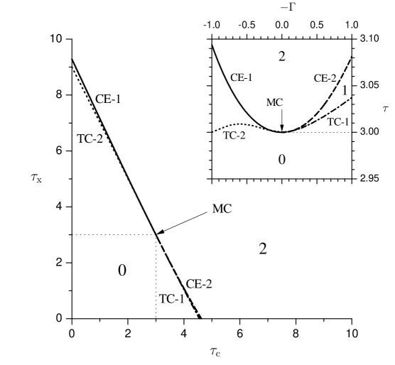
Figure 8: Single-chain phase diagram for the AISAT model ($\tau_{\mathrm{x}}$ vs $\tau_{\mathrm{c}}$ in the main graph and $\tau$ vs $-\Gamma$ in the inset). Lines and tags are defined as in Fig. 6.

In the $\tau_{\mathrm{x}}$ vs $\tau_{\mathrm{c}}$ diagram, the collapse transition looks like a single line passing through the MC point (which occurs for ${\tau_{\mathrm{x}}=\tau_{\mathrm{c}}=3}$), separating the swollen state from the highly-compact state. Nevertheless, the mapping on the alternative parameters $\tau$ and $\Gamma$ (Fig. 8 inset) reveals the fine structure of this “line”. In fact, for ${\tau_{\mathrm{c}}>\tau_{\mathrm{x}}}$, the transition line splits into two different lines of TC-1 and CE-2 points, whereas for ${\tau_{\mathrm{c}}<\tau_{\mathrm{x}}}$ it turns out to be a line of CE-1 points, which is, a first-order collapse. The similarity of the $\tau$ vs $-\Gamma$ diagram for the AISAT model with the $\tau$ vs $\omega$ diagram of the Wu-Bradley model is now evident. The most relevant difference is that, in the latter case, the TC-1 and CE-2 lines become well separated for large $\omega$ values, whereas, in the former case, they remain very close to each other over the whole range of admissible $\Gamma$ values. In Figs. 9 and 10 we report grand-canonical phase diagrams for the two special cases ${\tau_{\mathrm{x}}=1}$ and ${\tau_{\mathrm{c}}=1}$, respectively.

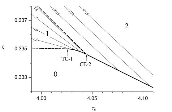
Figure 9: Grand-canonical phase diagram ($\zeta$ vs $\tau_{\mathrm{c}}$) for ${\omega=1}$ and ${\tau_{\mathrm{x}}=1}$ (colliding model). Lines and tags are as in previous figures.

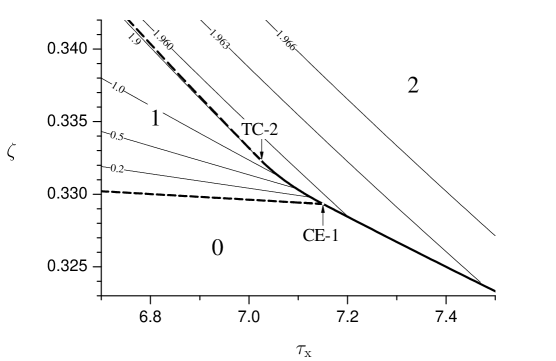
Figure 10: Grand-canonical phase diagram ($\zeta$ vs $\tau_{\mathrm{x}}$) for ${\omega=1}$ and ${\tau_{\mathrm{c}}=1}$ (crossing model). Lines and tags as in previous figures.

This two cases have been respectively denoted as colliding model and crossing model Bedini et al. (2013a), since either only collisions or only crossings are energetically favored, even though both collisions and crossings are always allowed. We can fully appreciate the analogy with the ${\omega>1}$ and ${\omega<1}$ cases of the Wu-Bradley model (Figs. 3 and 4, respectively), even though at a much smaller energy scale.

V Discussion and conclusions

Let us now discuss our results, with special attention to comparing them with those appeared in the literature for corresponding two-dimensional models.

As far as the Wu-Bradley model (${\tau_{\mathrm{x}}=\tau_{\mathrm{c}}}$) is concerned, we have obtained a nice agreement with the (single-chain) phase diagram proposed by Bedini and coworkers Bedini et al. (2014). The 0-2 transition (CE-1 line in Fig. 6) is conjectured to be first order, in agreement with our prediction. Moreover, the 0-1 transition is conjectured to be in the ISAW-theta universality class, and, even though in this case we cannot give a corresponding prediction for critical exponents, we find it significant that our 0-1 transition line is indeed made up of tricritical (TC-1) points. Note also that for ${\tau=0}$ (ISAW model) the TC-1 point occurs at ${\omega\approx 1.55}$, to be compared with the theta point of the 2d square lattice model, occurring at ${\omega\approx 1.95}$ Caracciolo et al. (2011). Finally, the 1-2 transition is not characterized precisely in the cited article, due to difficulties in simulating dense polymers, but there is reasonable evidence that it is a continuous transition, which is also in agreement with our prediction. On top of this, Bedini and coworkers identify the merging point of the above transitions with the ISAT collapse, characterized by specific properties (putatively, an infinite-order multicritical point Nahum et al. (2013)), which disappear as soon as an arbitrarily small contact interaction is introduced. There is indeed a striking analogy with the MC point of our Husimi-lattice model. We also find it noticeable that the Husimi-lattice solution reproduces some fine details of the 2d phase diagram, for instance, the slight positive slope of the CE-1 line and the precise location of the MC point.

As far as the AISAT model (${\omega=1}$) is concerned, the situation is more involved. For the case of preferred crossings (${\tau_{\mathrm{c}}<\tau_{\mathrm{x}}}$), our prediction, that the collapse transition becomes first order, agrees with Foster’s transfer-matrix results Foster (2011). In the cited reference, it is not possible to estimate the precise point at which the change of regime takes place, but the results seem to be compatible with our scenario. Unfortunately, the first-order transition is not confirmed by Bedini and coworkers’ simulations Bedini et al. (2013a), which conversely predict, for the crossing model (${\tau_{\mathrm{c}}=1}$), an ISAW-like transition, with a moderately compact collapsed state. Let us note that, probably with an eye to Foster’s findings, the latter authors report having observed some evidence of a multiply-peaked probability distribution, which seems nonetheless to become unimodal at large lengths. Our scenario might be compatible with such not fully definite results, because the close proximity of the TC-2 point (where the 1-2 transition becomes critical) to the CE-1 point (see Fig. 10) implies a very weak free-energy barrier, which might in fact give rise to a broad probability distribution, rather than two sharp peaks. Note indeed in Fig. 4 the much larger distance between the TC-2 and CE-1 points for the Wu-Bradley model with ${\omega=0.5}$, where the first-order transition is clearly pointed out by the simulation Bedini et al. (2014).

In the opposite case of preferred collisions (${\tau_{\mathrm{c}}>\tau_{\mathrm{x}}}$), a comparison with 2d findings presents even more difficulties. Our results predict a two-stage collapse, with a TC-1 point followed by a CE-2 point (see Fig. 9). As mentioned in the text, both these points correspond to continuous transitions, the former (which we have conjectured to be ISAW-like) toward a moderately-compact state, and the latter toward a highly-compact one. Again, due to the close proximity of the two points in the parameters space, we believe that such a scenario is not incompatible with Bedini and coworkers’ simulations Bedini et al. (2013a), predicting a highly-dense collapsed phase for the colliding model (${\tau_{\mathrm{x}}=1}$). On the other hand, Foster’s transfer-matrix results Foster (2011) seem to suggest that the ISAT critical properties extend to the whole range of preferred collisions (or penalized crossings) ${\tau_{\mathrm{c}}\geq\tau_{\mathrm{x}}>0}$, but the validity of these results (for the pure ISAT case itself Foster (2009)) has recently been questioned, by means of field-theoretic arguments Nahum et al. (2013), pointing out the presence of very strong logarithmic corrections.

The limiting case ${\tau_{\mathrm{x}}=0}$ (VISAW model) is worth a separate discussion, because in this case an exact solution Warnaar et al. (1992) of the corresponding $O(n)$ model (due to Blöte and Nienhuis Blöte and Nienhuis (1989)) points out a specific universality class, different from that of the ISAW. The critical exponent values predicted by the exact solution turn out to be quite elusive, since transfer-matrix approaches Blöte and Nienhuis (1989); Foster and Pinettes (2012) give incompatible results, whereas Monte Carlo simulations Bedini et al. (2013b) are almost compatible (at least for the $\nu$ exponent) with the ISAW universality class itself. A careful investigation of the Blöte-Nienhuis theta state, recently performed by Vernier, Jacobsen, and Saleur Vernier et al. (2015), suggests that so difficult numerical estimates might arise from the peculiar nature of the associated conformal field theory, characterized by a continuous spectrum of critical exponents. In order to reconcile our phase diagram for the VISAW case (in fact practically equivalent to that of Fig. 9) with the exact results, we should postulate that the actual collapse transition is indeed the TC-1 point, so that the Blöte-Nienhuis theta state should be associated to a different object, which we might tentatively identify with the CE-2 point. Of course, on the sole basis of our arguments, this possibility is nothing more than speculation, but we find it quite intriguing, because it seems not to be inconsistent with the most up-to-date results Vernier et al. (2015), still inconclusive about the role of the different integrable points in the phase diagram. On the other hand, a slight evidence supporting our interpretation is provided by the fact that the Blöte-Nienhuis point is characterized by a nonzero density Foster and Pinettes (2003); Vernier et al. (2015), and that, approached upon increasing fugacity, it corresponds to a discontinuous transition Vernier et al. (2015). Both features qualitatively agree with our predictions for the CE-2 point.

Let us finally spend a few words about the analytical technique that we have used in this article. Even though the solution of Husimi and Bethe lattice models is a very standard technique Lavis and Bell (1999), we would like to emphasize that our variational-free-energy approach considerably simplifies the derivation of the recursion equations, which may be of use in particular when dealing with models of considerable complexity like the current one. This approach is not fully original, because it has been demonstrated for instance in certain specialized literature dealing with spin glasses (where a quenched variational free energy is considered) Mezard and Parisi (2001), but, to the best of our knowledge, it has never been practically exploited, at least in the context of polymer models Pretti (2002); Serra et al. (2004); Zara and Pretti (2007); Oliveira et al. (2008); Neto and Stilck (2013); Lise et al. (1998); Buzano and Pretti (2002); Pretti (2006); Serra and Stilck (2007); Neto and Stilck (2008).

Appendix A Recursion equations

In this Appendix, we shall report a detailed derivation of the recursion equations for the Husimi-lattice model.

Table 1: The first row reports the possible configurations of the polymer on a lattice site, with $w_{i}$ denoting the corresponding cavity fields associated to the two branches attached to the site (top-right and bottom-left corners). The “prime” symbol in parentheses denotes the possibility of both fields $w_{2^{\vphantom{\prime}}}$ and $w_{2^{\prime}}$. The second row reports the contribution of each site to the site partition function $z$ (see the text).

$w_{0^{\vphantom{\prime}}}^{2}$	$\frac{1}{4}w_{1^{\vphantom{\prime}}}^{2}$	$\frac{1}{4}w_{1^{\vphantom{\prime}}}^{2}$	$\frac{1}{4}w_{1^{\vphantom{\prime}}}^{2}$	$\frac{1}{4}w_{1^{\vphantom{\prime}}}^{2}$	$w_{2^{\vphantom{\prime}}}^{\vphantom{1}}w_{0^{\prime}}^{\vphantom{1}}$	$w_{2^{\vphantom{\prime}}}^{\vphantom{1}}w_{0^{\prime}}^{\vphantom{1}}$	$\tau_{\mathrm{c}}w_{2^{\vphantom{\prime}}}^{2}$	$\tau_{\mathrm{c}}\left(w_{2^{\vphantom{\prime}}}^{2}+2w_{2^{\vphantom{\prime}}}^{\vphantom{1}}w_{2^{\prime}}^{\vphantom{1}}\right)$	$\tau_{\mathrm{x}}\left(w_{2^{\vphantom{\prime}}}^{2}+2w_{2^{\vphantom{\prime}}}^{\vphantom{1}}w_{2^{\prime}}^{\vphantom{1}}\right)$

In Table 1 we report all possible site configurations, along with the cavity fields associated to the two attached branches. The association rules between fields and configurations are as follows. First of all, $w_{n}$ is associated to a configuration with $n$ segments incident from the branch, for $n=0,1,2$. Moreover, $w_{0}$ and $w_{0^{\prime}}$ distinguish whether the site is empty or visited, respectively. Finally, $w_{2^{\prime}}$ represents the case in which the two incident segments are connected by a loop whose number of steps does not diverge in the thermodynamic limit, whereas $w_{2}$ represents all other cases, namely, either the segments are connected by a macroscopic loop or they are not connected. Note that a single segment incident from a branch can arrive from two different directions. Since in the absence of stiffness we expect the two possibilities to be equivalent (i.e., the system to be isotropic), we assume $w_{1}$ to be the total weight of both, so that a single one has weight ${\frac{1}{2}w_{1}}$.

The second row of Table 1 reports the terms of $z$ corresponding to each configuration. The last two terms take into account the possibility of a finite loop ($w_{2^{\prime}}$ field) in one of the two branches, or neither of them, but not both. In conclusion, the single-site partition function reads

$$z=w_{0}^{2}+w_{1}^{2}+2w_{2}^{\vphantom{1}}\left[w_{0^{\prime}}^{\vphantom{1}}+(\tau_{\mathrm{c}}+\tau_{\mathrm{x}})w_{2^{\prime}}^{\vphantom{1}}\right]+(2\tau_{\mathrm{c}}+\tau_{\mathrm{x}})w_{2}^{2}\,.$$ (17)

Let us observe that $w_{0^{\prime}}$ and $w_{2^{\prime}}$ appear only in the linear combination $w_{0^{\prime}}+(\tau_{\mathrm{c}}+\tau_{\mathrm{x}})w_{2^{\prime}}$. We argue that this will be a general feature of our equations, because this linear combination represents the total weight of configurations such that the polymer enters a given branch and exits after a finite number of steps. In particular, $w_{0^{\prime}}$ can be regarded as the zero-step case, in which the polymer visits only the root site of the branch (without a collision), whereas the latter term includes all other cases. The above observation motivates the definition of a “composite” cavity field, namely,

$$w_{3}\equiv w_{0^{\prime}}+(\tau_{\mathrm{c}}+\tau_{\mathrm{x}})w_{2^{\prime}}\,,$$ (18)

so that the single-site partition function can be rewritten as

$$z=w_{0}^{2}+w_{1}^{2}+2w_{2}^{\vphantom{1}}w_{3}^{\vphantom{1}}+(2\tau_{\mathrm{c}}+\tau_{\mathrm{x}})w_{2}^{2}\,.$$ (19)

As far as the cluster partition function is concerned, let us first observe that we can write

$$q=\sum_{n=0}^{4}q_{n}\zeta^{n}\,,$$ (20)

where $\zeta$ is the fugacity and $q_{n}$ can be denoted as the canonical cluster partition function for a cluster with $n$ segments. According to (9), the segment density will therefore take the form

$$\rho=\frac{1}{2q}\sum_{n=0}^{4}nq_{n}\zeta^{n}\,.$$ (21)

In Table 2 we report the possible arrangements of polymer segments on a square cluster, along with the corresponding cavity fields.

Table 2: The first row reports the possible arrangements of polymer segments on a square cluster, and the corresponding cavity fields. The second row reports the number $n$ of polymer segments in each case. The third row reports the multiplicity $m$ of each arrangement, i.e., the number of different configurations that can be generated by rotations.

$n$	$0$	$1$	$2$	$2$	$3$	$4$
$m$	$1$	$4$	$4$	$2$	$4$	$1$

We can identify the following rules.

Let $\kappa$ be the number of segments placed on a given corner of the square.

(i) If ${\kappa=0}$, then the possible fields are $w_{0}$ and $w_{2}$. In the former case the corner site is empty. In the latter case the corner site is visited once, by a walk along the corner outside the cluster; there can occur contacts ($\omega$ weight) with other visited sites of the cluster.

(ii) If ${\kappa=1}$, then the only possible field is $w_{1}$. The site is visited once, by a walk that exits (or enters) the cluster; contacts can occur with other visited sites.

(iii) If ${\kappa=2}$, then the possible fields are $w_{3}$ and $w_{2}$. In the former case the site is visited either once, by a walk along the corner inside the cluster, or twice, by a walk that exits the cluster and re-enters after a finite number of steps. In the latter case the site is visited twice. Note that the $w_{2}$ field does not incorporate Boltzmann weights of crossing or collisions occurring at the corner site, whereas the $w_{3}$ field does. The complete field combination for the case ${\kappa=2}$ is therefore ${(2\tau_{\mathrm{c}}+\tau_{\mathrm{x}})w_{2}+w_{3}}$.

The above rules, together with Table 2, explain the following expressions:

$$\!\!\!\!\!q_{0}^{\vphantom{1}}=w_{0}^{4}+4w_{0}^{3}w_{2}^{\vphantom{1}}+(4\omega+2)w_{0}^{2}w_{2}^{2}+4\omega^{2}w_{0}^{\vphantom{1}}w_{2}^{3}+\omega^{4}w_{2}^{4}\,,$$

$$\!\!\!\!\!q_{1}^{\vphantom{1}}=4\,w_{1}^{2}\left(w_{0}^{2}+2\omega w_{0}^{\vphantom{1}}w_{2}^{\vphantom{1}}+\omega^{3}w_{2}^{2}\right)^{\vphantom{1}}\,,$$

$$\!\!\!\!\!q_{2}^{\vphantom{1}}=4\,w_{1}^{2}\left(w_{0}^{\vphantom{1}}+\omega^{2}w_{2}^{\vphantom{1}}\right)\left[(2\tau_{\mathrm{c}}+\tau_{\mathrm{x}})w_{2}^{\vphantom{1}}+w_{3}^{\vphantom{1}}\right]^{\vphantom{1}}+2\,\omega^{2}w_{1}^{4}\,,$$

$$\!\!\!\!\!q_{3}^{\vphantom{1}}=4\,\omega w_{1}^{2}\left[(2\tau_{\mathrm{c}}+\tau_{\mathrm{x}})w_{2}^{\vphantom{1}}+w_{3}^{\vphantom{1}}\right]^{2}\,,$$

$$\!\!\!\!\!q_{4}^{\vphantom{1}}=\left[(2\tau_{\mathrm{c}}+\tau_{\mathrm{x}})w_{2}^{\vphantom{1}}+w_{3}^{\vphantom{1}}\right]^{4}-\left(\tau_{\mathrm{c}}w_{2}^{\vphantom{1}}+w_{3}^{\vphantom{1}}\right)^{4}\,.$$

(22)

With respect to the previous discussion, the only extra ingredient is that we must subtract from the expression of $q_{4}$ the weight of configurations with finite-length loops (namely, ${\tau_{\mathrm{c}}w_{2}+w_{3}}$) on all four corners. Note that ${\tau_{\mathrm{c}}w_{2}}$ is the weight associated to the presence of a walk along the corner inside the square, colliding with a (macroscopic) walk outside.

Let us now also report explicitly the recursion functions $f_{i}$ appearing in equation (7). Due to the form (20) of the cluster partition function, they take the similar form

$$f_{i}=\sum_{n=0}^{4}f_{i,n}\zeta^{n}\,.$$ (23)

The explicit expressions of $f_{i,n}$ turn out to be:

$$f_{0,0}^{\vphantom{1}}=w_{0}^{3}+3w_{0}^{2}w_{2}^{\vphantom{1}}+(2\omega+1)w_{0}^{\vphantom{1}}w_{2}^{2}+\omega^{2}w_{2}^{3}\,,$$

$$f_{0,1}^{\vphantom{1}}=2w_{1}^{2}\left(w_{0}^{\vphantom{1}}+\omega w_{2}^{\vphantom{1}}\right)\,,$$

$$f_{0,2}^{\vphantom{1}}=w_{1}^{2}\left[(2\tau_{\mathrm{c}}+\tau_{\mathrm{x}})w_{2}^{\vphantom{1}}+w_{3}^{\vphantom{1}}\right]\,,$$

$$f_{0,3}^{\vphantom{1}}=0\,,$$

$$f_{0,4}^{\vphantom{1}}=0\,;$$ (24)

$$f_{1,0}^{\vphantom{1}}=0\,,$$

$$f_{1,1}^{\vphantom{1}}=2w_{1}^{\vphantom{1}}\left(w_{0}^{2}+2\omega w_{0}^{\vphantom{1}}w_{2}^{\vphantom{1}}+\omega^{3}w_{2}^{2}\right)\,,$$

$$f_{1,2}^{\vphantom{1}}=2w_{1}^{\vphantom{1}}\left(w_{0}^{\vphantom{1}}+\omega^{2}w_{2}^{\vphantom{1}}\right)\left[(2\tau_{\mathrm{c}}+\tau_{\mathrm{x}})w_{2}^{\vphantom{1}}+w_{3}^{\vphantom{1}}\right]+2\omega^{2}w_{1}^{3}\,,$$

$$f_{1,3}^{\vphantom{1}}=2\omega w_{1}^{\vphantom{1}}\left[(2\tau_{\mathrm{c}}+\tau_{\mathrm{x}})w_{2}^{\vphantom{1}}+w_{3}^{\vphantom{1}}\right]{\!}^{2}\,,$$

$$f_{1,4}^{\vphantom{1}}=0\,;$$ (25)

$$f_{2,0}^{\vphantom{1}}=0\,,$$

$$f_{2,1}^{\vphantom{1}}=0\,,$$

$$f_{2,2}^{\vphantom{1}}=w_{1}^{2}\left(w_{0}^{\vphantom{1}}+\omega^{2}w_{2}^{\vphantom{1}}\right)\,,$$

$$f_{2,3}^{\vphantom{1}}=2\omega w_{1}^{2}\left[(2\tau_{\mathrm{c}}+\tau_{\mathrm{x}})w_{2}^{\vphantom{1}}+w_{3}^{\vphantom{1}}\right]\,,$$

$$f_{2,4}^{\vphantom{1}}=\left[(2\tau_{\mathrm{c}}+\tau_{\mathrm{x}})w_{2}^{\vphantom{1}}+w_{3}^{\vphantom{1}}\right]{\!}^{3}-\left(\tau_{\mathrm{c}}w_{2}^{\vphantom{1}}+w_{3}^{\vphantom{1}}\right){\!}^{3}\,;$$ (26)

$$f_{3,0}^{\vphantom{1}}=w_{0}^{3}+(2\omega+1)w_{0}^{2}w_{2}^{\vphantom{1}}+3\omega^{2}w_{0}^{\vphantom{1}}w_{2}^{2}+\omega^{4}w_{2}^{3}\,,$$

$$f_{3,1}^{\vphantom{1}}=2\omega w_{1}^{2}\left(w_{0}^{\vphantom{1}}+\omega^{2}w_{2}^{\vphantom{1}}\right)\,,$$

$$f_{3,2}^{\vphantom{1}}=\omega^{2}w_{1}^{2}\left[(2\tau_{\mathrm{c}}+\tau_{\mathrm{x}})w_{2}^{\vphantom{1}}+w_{3}^{\vphantom{1}}\right]\,,$$

$$f_{3,3}^{\vphantom{1}}=0\,,$$

$$f_{3,4}^{\vphantom{1}}=(\tau_{\mathrm{c}}+\tau_{\mathrm{x}})\left(\tau_{\mathrm{c}}w_{2}^{\vphantom{1}}+w_{3}^{\vphantom{1}}\right){\!}^{3}\,.$$ (27)

Let us note that we have obtained the above formulas by a trivial exercise of derivatives, but, as mentioned in the text, they can also be interpreted in terms of self-similarity conditions. Indeed, this is the more usual (recursive) route followed for this kind of calculations, at least in the context of polymer models. For this reason we felt it appropriate to set out also these formulas in full detail.

As mentioned in the text, the numerical technique we employ to solve the recursion equations is a simple fixed-point method. Given a tentative set of cavity fields $w_{0},\dots,w_{3}$ (which we shall collectively denote as $w$ in the following formulas), a new estimate of each field can be computed, according to equation (7), by an expression of the form

$$\hat{w}_{i}(w)=\frac{f_{i}(w)}{\sum_{k=0}^{3}f_{k}(w)}\,,$$ (28)

where the denominator takes into account the normalization condition (8).

A second-order phase transition is characterized by the fact that a minimum of the free energy becomes a saddle point, so that the corresponding thermodynamic equilibrium state is no longer stable. Thermodynamic (in)stability is reflected in the (in)stability of the fixed point of the recursion equations. Therefore, in order to determine second-order transitions with good precision, it is convenient to analyze the eigenvalues of the Jacobian matrix associated with the recursion equations and the conditions in which any eigenvalue equals unity. According to equation (28), the elements of such a Jacobian matrix can be written as

$$\frac{\partial\hat{w}_{i}}{\partial w_{j}}(w)=\frac{\frac{\partial f_{i}}{\partial w_{j}}(w)-\hat{w}_{i}(w)\sum_{k=0}^{3}\frac{\partial f_{k}}{\partial w_{j}}(w)}{\sum_{k=0}^{3}f_{k}(w)}\,.$$ (29)

The derivatives of $f_{i}(w)$ can be determined from equations (23)–(27). As far as the transition lines are concerned, we can locate them numerically as loci of zeroes of $\det(J-I)$, where $J$ is the Jacobian matrix and $I$ the identity matrix. This can be safely done, because the peculiar form of the recursion equations allows us to follow a given solution (fixed point) even in the parameter region where it becomes unstable. More specifically, if one starts with tentative fields satisfying ${w_{1}=w_{2}=0}$ (which characterizes the 0 phase), the new estimates computed by equation (28) turn out to satisfy rigorously the same condition. The same holds for the 2 phase, characterized by the sole condition ${w_{1}=0}$.

Appendix B Bethe lattice solution

We shall now discuss the solution of the model on the Bethe lattice. This solution is interesting in particular for the Wu-Bradley model, because the whole phase diagram, which turns out to be qualitatively equivalent to that of the Husimi lattice case, can be worked out analytically, including the peculiar features of the MC point. Let us remind that the Bethe lattice can be viewed as a thermodynamic limit of a random-regular graph, the latter being defined as a random graph (with ordinary pairwise edges) with fixed coordination number. Like the Husimi lattice, the Bethe lattice can be treated locally as if it were a tree-graph, because the length of closed paths diverges (logarithmically) with the system size. Still with the idea of approximating the 2d square lattice model, we choose a coordination number $4$. Let us warn the reader that, throughout the following calculations, we shall use the same symbols used for the Husimi lattice case, sometimes with a slightly different physical meaning.

The free energy density per lattice bond can still be written in the form

$$\psi=-\frac{1}{2}\ln q+\ln z\,,$$ (30)

where now $q$ is star-cluster partition function (where a star cluster can be defined as a set of lattice bonds incident to a given site), $z$ is the single-bond partition function, and $1/2$ is the ratio between the number of star clusters and the number of bonds present in the system. In analogy to the Husimi lattice solution, the single-bond term may be viewed as a correction over the cluster term, due to the overlap between clusters.

Table 3: Possible configurations of the polymer on a Bethe lattice site: $w_{i}$ denote the cavity fields associated to the four branches attached to the site (one for each nearest-neighbor). The “prime” symbol in parentheses denotes the possibility of both fields $w_{0^{\vphantom{\prime}}}$ and $w_{0^{\prime}}$. The expressions below each figure are the respective contributions (including multiplicity) to the star-cluster partition function $q$.

$(w_{0^{\vphantom{\prime}}}^{\vphantom{1}}+w_{0^{\prime}}^{\vphantom{1}})^{4}$	$2\zeta^{2}w_{1^{\vphantom{\prime}}}^{2}(w_{0^{\vphantom{\prime}}}^{\vphantom{1}}+\omega w_{0^{\prime}}^{\vphantom{1}})^{2}$	$4\zeta^{2}w_{1^{\vphantom{\prime}}}^{2}(w_{0^{\vphantom{\prime}}}^{\vphantom{1}}+\omega w_{0^{\prime}}^{\vphantom{1}})^{2}$
$2\tau_{\mathrm{c}}\zeta^{4}w_{1^{\vphantom{\prime}}}^{4}$	$\tau_{\mathrm{x}}\zeta^{4}w_{1^{\vphantom{\prime}}}^{4}$

In Table 3 we sketch possible configurations of the polymer on a lattice site, along with the cavity fields associated to its nearest neighbors (i.e., the root sites of the four branches attached to the given site). Note that each figure represents indeed a multiplicity of configurations, that can be obtained from one another by rotations. The cavity fields are defined as follows: $w_{n}$ is associated to a configuration with ${n=0,1}$ segments incident from a root site, whereas $w_{0}$ and $w_{0^{\prime}}$ distinguish whether the root site is empty or visited, respectively. The terms of the star-cluster partition function $q$, corresponding to each configuration, are also reported in Table 3. Summing these terms, we obtain

$$q=(w_{0}^{\vphantom{1}}+w_{0^{\prime}}^{\vphantom{1}})^{4}+6\zeta^{2}w_{1}^{2}(w_{0}^{\vphantom{1}}+\omega w_{0^{\prime}}^{\vphantom{1}})^{2}+(2\tau_{\mathrm{c}}+\tau_{\mathrm{x}})\zeta^{4}w_{1}^{4}\,.$$ (31)

As far as the single-bond partition function is concerned, we have

$$z=w_{0}^{2}+2w_{0}^{\vphantom{1}}w_{0^{\prime}}^{\vphantom{1}}+\omega w_{0^{\prime}}^{2}+\zeta w_{1}^{2}\,,$$ (32)

which can be explained as follows. The first three terms correspond to an empty lattice bond, where the two neighboring sites are, respectively, both empty, one visited and one empty, or both visited. The last term takes into account the case of a bond visited by a polymer segment, both neighboring sites being obviously visited as well.

We are now in a position to work out the model solution, since all the needed information is contained in equations (30), (31), and (32). Setting at zero the free-energy derivatives with respect to the cavity fields, we obtain the self-consistency equations

$$w_{0\hphantom{{}^{\prime}}}^{\vphantom{1}}\propto(w_{0}^{\vphantom{1}}+w_{0^{\prime}}^{\vphantom{1}})^{3}\,,$$ (33)

$$w_{0^{\prime}}^{\vphantom{1}}\propto 3\zeta^{2}w_{1}^{2}(w_{0}^{\vphantom{1}}+\omega w_{0^{\prime}}^{\vphantom{1}})\,,$$ (34)

$$w_{1\hphantom{{}^{\prime}}}^{\vphantom{1}}\propto 3\zeta w_{1}^{\vphantom{1}}(w_{0}^{\vphantom{1}}+\omega w_{0^{\prime}}^{\vphantom{1}})^{2}+(2\tau_{\mathrm{c}}+\tau_{\mathrm{x}})\zeta^{3}w_{1}^{3}\,.$$ (35)

As previously mentioned, these equations can also be interpreted as self-similarity conditions, where the proportionality constant remains undetermined, because of the invariance of $\psi$ under multiplication of each cavity field by a constant. Thermal averages can be evaluated as derivatives of the free energy, and in particular the average number of segments (segment density) per bond reads

$$\rho=-\frac{\partial\psi}{\partial\ln\zeta}\,.$$ (36)

Exploiting as usual the fact that the derivatives of $\psi$ with respect to the cavity fields vanish at equilibrium points, we arrive at

$$\rho=\frac{\zeta w_{1}^{2}}{z}\,.$$ (37)

The last simple expression can also be rationalized from the previous explanation of the various terms appearing in the single-bond partition function.

Let us observe that in all the previous equations, the collision and crossing activities $\tau_{\mathrm{c}}$ and $\tau_{\mathrm{x}}$ always appear only in the combination ${2\tau_{\mathrm{c}}+\tau_{\mathrm{x}}}$. As a consequence, using the $\tau$ and $\Gamma$ parameters defined by equations (12) and (13) (as we shall do in the following calculations), the model turns out to depend only on the average $\tau$, being thus completely unaffected by the asymmetry parameter $\Gamma$. This means that the Bethe lattice model, at odds with the Husimi lattice one, does not exhibit any “fine structure” in the asymmetric case ${\tau_{\mathrm{x}}\neq\tau_{\mathrm{c}}}$.

B.1 Critical 0-1 transition and TC-1 point

It can be easily verified that the self-consistency equations (33)–(35) always admit a solution with ${w_{0^{\prime}}=w_{1}=0}$ (and therefore ${\rho=0}$), whereas $w_{0}$ depends on the normalization condition. In the following, we shall choose the latter as ${z=1}$, so that (32) implies ${w_{0}=1}$, whence (31) and (30) trivially lead to

$$\psi=0\,.$$ (38)

This solution is obviously identified with the 0 phase.

In the event of a critical transition (to the 1 phase), we expect that $w_{0^{\prime}}$ and $w_{1}$ are small near the transition line, whereas ${w_{0}\approx 1}$. Let us define the ratios ${x\equiv w_{0^{\prime}}/w_{0}}$ and ${y\equiv w_{1}/w_{0}}$. From (33)–(35) we can derive two self-consistency equations for $x$ and $y$, namely,

$$x=\frac{3\zeta^{2}y^{2}(1+\omega x)}{(1+x)^{3}}\,,$$ (39)

$$y=\frac{3\zeta y(1+\omega x)^{2}+3\tau\zeta^{3}y^{3}}{(1+x)^{3}}\,,$$ (40)

which no longer depend on the arbitrary normalization. For small $x$, we have respectively

$$x=3\zeta^{2}y^{2}[1+\mathcal{O}(x)]\,,$$ (41)

$$y=3\zeta y[1+(2\omega-3)x+\mathcal{O}(x^{2})]+3\tau\zeta^{3}y^{3}[1+\mathcal{O}(x)]\,.$$

(42)

Equation (41) confirms that also $y$ must be small, and it shows in particular that $x=\mathcal{O}(y^{2})$. As a consequence, it can also be rewritten as

$$x=3\zeta^{2}y^{2}+\mathcal{O}(y^{4})\,.$$ (43)

Replacing the latter equation into (42), we finally obtain a self-consistency equation for $y$ alone (valid for small $y$), namely

$$y=3\zeta y+3\left[3\left(2\omega-3\right)+\tau\right]\zeta^{3}y^{3}+\mathcal{O}(y^{5})\,.$$ (44)

The criticality condition (0-1 transition line) occurs when the coefficient of the degree-1 term on the right-hand side equals unity, that is for

$$\zeta=\frac{1}{3}\,.$$ (45)

Furthermore, the transition changes from second to first order (TC-1 point) when the degree-3 term vanishes, which happens for

$$\tau=9-6\omega\,.$$ (46)

In the single-chain phase diagram $\tau$ vs $\omega$, the latter equation represents the line of continuous transitions between the swollen state and the ordinary compact state (TC-1 line). This line turns out to be numerically quite close to the homologous line determined for the Husimi lattice model (see Fig. 11).

Figure 11: Single-chain phase diagram ($\tau$ vs $\omega$) for the Bethe lattice model. Lines and tags as in Fig. 6. Thin lines represent the Husimi lattice results for the Wu-Bradley model.

B.2 Critical 1-2 transition and TC-2 point

Equations (33)–(35) also admit a solution with ${w_{0}=w_{0^{\prime}}=0}$. With ${z=1}$, equations (37) and (32) imply ${\rho=\zeta w_{1}^{2}=1}$, whence (31) and (30) lead to

$$\psi=-{\textstyle\frac{1}{2}}\ln\,(3\tau\zeta^{2})\,.$$ (47)

This solution can be identified with the 2 phase. Note that a density of exactly $1$ segment per lattice bond means that all lattice sites are doubly visited, i.e., on the Bethe lattice this is actually a saturated phase, which was not the case on the Husimi lattice.

In the event of a critical transition (to the 1 phase), we expect that $w_{0}$ and $w_{0^{\prime}}$ are small near the transition line, whereas ${w_{1}\approx 1/\sqrt{\zeta}}$. Let us define the ratios ${a\equiv w_{0}/w_{1}}$ and ${b\equiv w_{0^{\prime}}/w_{1}}$. As in the previous case, equations (33)–(35) allow us to derive two recursion equations for $a$ and $b$, namely,

$$a=\frac{(a+b)^{3}}{3\zeta(a+\omega b)^{2}+3\tau\zeta^{3}}\,,$$ (48)

$$b=\frac{\zeta(a+\omega b)}{(a+\omega b)^{2}+\tau\zeta^{2}}\,.$$ (49)

For small $b$, from equation (48) one can easily argue that ${a=\mathcal{O}(b^{3})}$, which, replaced into the same equation, leads to

$$a=\frac{1}{3\tau\zeta^{3}}b^{3}+\mathcal{O}(b^{5})\,.$$ (50)

Plugging this equation into (49), we obtain a self-consistency equation for $b$ alone (valid for small $b$), namely,

$$b=\frac{\omega}{\tau\zeta}b+\frac{1-3\omega^{3}\zeta}{3\tau^{2}\zeta^{4}}b^{3}+\mathcal{O}(b^{5})\,.$$ (51)

The criticality condition (1-2 transition line) occurs when the coefficient of the degree-1 term on the right-hand side equals unity, that is for

$$\zeta=\frac{\omega}{\tau}\,.$$ (52)

The TC-2 point occurs when we add the condition that the degree-3 term vanishes:

$$\zeta=\frac{1}{3\omega^{3}}\,.$$ (53)

Putting these conditions together, we obtain

$$\tau=3\omega^{4}\,,$$ (54)

which represents the TC-2 line in the single-chain phase diagram (see Fig. 11). Note that also this line turns out to be rather close to the analogous one computed for the Husimi lattice model.

B.3 First-order 0-2 transition, CE and MC points

In the previous two subsections, we have argued that the 0 and 2 phases are characterized by constant density values (${\rho=0}$ and ${\rho=1}$, respectively), which implies that there cannot exist a continuous phase transition between them. Conversely, a first-order transition exists, and it can be determined by equating the free energies (38) and (47), which yields

$$\zeta=\frac{1}{\sqrt{3\tau}}\,.$$ (55)

The CE-1 point occurs where the 0-2 transition line encounters the continuous 0-1 transition line (see Fig. 4), so that it is defined by the simultaneous solution of equations (55) and (45). Eliminating $\zeta$, we obtain

$$\tau=3\,,$$ (56)

which is denoted as CE-1 line in Fig. 11. The CE-2 point occurs where the 0-2 transition line meets the continuous 1-2 transition line (see Fig. 3). This is determined by the simultaneous solution of equations (55) and (52). Eliminating $\zeta$, we now obtain

$$\tau=3\omega^{2}\,,$$ (57)

denoted as CE-2 line in Fig. 11. Finally, the MC point occurs in the event of a simultaneous merging of the 0-2 line with the (continuous) 0-1 and 1-2 lines (see Fig. 5). As a consequence, it is defined by the simultaneous solution of equations (45), (52), and (55), or equivalently of (56) and (57), yielding

$$\omega=1\,,\,\tau=3\,.$$ (58)

It is noticeable that the MC point is the unique transition point, whose location in the phase diagram remains precisely the same for both the Husimi and Bethe lattice models, besides being also equal to the conjectured location of the ISAT collapse transition for the ordinary 2d square lattice.

B.4 ISAT model

Figure 12: Grand-canonical phase diagram ($\zeta$ vs $\tau$) for the pure ISAT model (${\omega=1}$) on the Bethe lattice. Lines and phase tags as in Fig. 5. Thin lines represent the Husimi lattice results. The inset displays the variational free-energy density (64) as a function of $\alpha$ (see the text), at the points tagged by A, B, C.

Let us now focus on the special case ${\omega=1}$, which is, the pure ISAT model. The $\zeta$ vs $\tau$ phase diagram is reported in Fig. 12, where we can observe that the transition lines, determined analytically by equations (45), (52), and (55), are numerically very close to the corresponding ones for the Husimi lattice model. In particular, as far as the 0-2 transition is concerned, the numerical discrepancy is so small that it cannot be appreciated at the scale of the figure.

Let us note that, with ${\omega=1}$, the variational free-energy density $\psi$ can be expressed as a function of only two “modified” cavity fields, which we can define as

$$u\equiv w_{0}+w_{0^{\prime}}\,,$$ (59)

$$v\equiv w_{1}\sqrt{\zeta}\,.$$ (60)

According to such definitions, the star (31) and bond (32) partition functions become respectively

$$q={u}^{4}+6\zeta{v}^{2}{u}^{2}+3\tau\zeta^{2}{v}^{4}\,,$$ (61)

$$z={u}^{2}+{v}^{2}\,,$$ (62)

whereas $\psi$ is still expressed by (30). Due to linearity of (59) and (60), the free energy is still invariant under multiplication of $u$ and $v$ by a coefficient, so that we can then freely choose the $(u,v)$ vector to have a unit magnitude. As a consequence, it can be parameterized as function of a single angular coordinate $\alpha$ as

$$(u,v)=(\cos\alpha,\sin\alpha)\,,$$ (63)

with ${\alpha\in[0,\pi/2]}$, because $u$ and $v$ must be both nonnegative. Replacing equation (63) into (61) and (62), and then into (30), by simple algebra we arrive at

$$\psi=-{\textstyle\frac{1}{2}}\ln\left[1+{\textstyle\frac{1}{2}}(3\zeta-1)\sin^{2}(2\alpha)+(3\tau\zeta^{2}-1)\sin^{4}\alpha\right]\,.$$ (64)

Moreover, taking into account (60) and (37), we obtain

$$\rho=\sin^{2}\alpha\,.$$ (65)

In conclusion, both the free-energy density $\psi$ and the segment density $\rho$ have been expressed as functions of a unique variational parameter $\alpha$.

Equilibrium points can now be determined from equation (64) by setting at zero the derivative of $\psi$ with respect to $\alpha$. It turns out that two constant solutions exist, namely, ${\alpha=0}$ and ${\alpha=\pi/2}$, corresponding respectively to the 0 and 2 phases. Taking also into account (65), the third solution, corresponding to the 1 phase, can be characterized by

$$\tau=\frac{1}{\zeta}\left[1-\left(1-\frac{1}{3\zeta}\right)\left(\frac{1}{\rho}-1\right)\right]\,.$$ (66)

The latter equation can be regarded as a family of contour lines of the density $\rho$ in the $\zeta$ vs $\tau$ diagram. It is easily observed that all such lines pass through the MC point (58), in agreement with the result obtained numerically for the Husimi lattice model.

We are now also in a position to probe analytically (for the Bethe case) the peculiar characterization of the MC point that has been discussed in the text. Indeed, in equation (64) we see that the occurrence of the 0-2 transition condition (55) implies that the ${\sin^{4}\alpha}$ term vanishes. Therefore, the free energy barrier is due entirely to the ${\sin^{2}(2\alpha)}$ term, whose amplitude vanishes precisely at the MC point ${\zeta=1/3}$. In the inset of Fig. 12, we have reported $\psi$ as a function of $\alpha$ at different points in the $\zeta$ vs $\tau$ plane, namely, those tagged by A, B, C. Point A is located along the 0-2 first-order transition line, so that we can observe a free-energy barrier between two equivalent minima. Point B coincides with the MC point, so that we observe a vanishing barrier. Finally, point C is located in the region of the 1 phase, so that we can observe the absolute free-energy minimum at an intermediate density value. Note that, since the point is located slightly off the analytical continuation of the 0-2 transition line, the ${\sin^{4}\alpha}$ term no longer vanishes, so that the free energies of the (unstable) $0$ and $2$ phases become different.

References

- de Gennes (1979) P. G. de Gennes, Scaling Concepts in Polymer Physics (Cornell University Press, Ithaca, 1979).
- des Cloizeaux and Jannink (1990) J. des Cloizeaux and G. Jannink, Polymers in Solution: their Modelling and Structure (Clarendon Press, Oxford, 1990).
- Vanderzande (1998) C. Vanderzande, Lattice Models of Polymers (Cambridge University Press, Cambridge, 1998).
- Massih and Moore (1975) A. R. Massih and M. A. Moore, J. Phys. A: Math. Gen. 8, 237 (1975).
- Foster (2009) D. P. Foster, J. Phys. A: Math. Theor. 42, 372002 (2009).
- Blöte and Nienhuis (1989) H. W. J. Blöte and B. Nienhuis, J. Phys. A: Math. Gen. 22, 1415 (1989).
- Foster and Pinettes (2003) D. P. Foster and C. Pinettes, J. Phys. A: Math. Gen. 36, 10279 (2003).
- Bedini et al. (2013a) A. Bedini, A. L. Owczarek, and T. Prellberg, Phys. Rev. E 87, 012142 (2013a).
- Nahum et al. (2013) A. Nahum, P. Serna, A. M. Somoza, and M. Ortuño, Phys. Rev. B 87, 184204 (2013).
- Vernier et al. (2015) E. Vernier, J. L. Jacobsen, and H. Saleur, J. Stat. Mech. P09001 (2015).
- Duplantier and Saleur (1987) B. Duplantier and H. Saleur, Phys. Rev. Lett. 59, 539 (1987).
- Caracciolo et al. (2011) S. Caracciolo, M. Gherardi, M. Papinutto, and A. Pelissetto, J. Phys. A: Math. Theor. 44, 115004 (2011).
- Meirovitch and Lim (1988) H. Meirovitch and H. A. Lim, Phys. Rev. A 38, 1670 (1988).
- Owczarek and Prellberg (2007) A. L. Owczarek and T. Prellberg, Physica A 373, 433 (2007).
- Bedini et al. (2013b) A. Bedini, A. L. Owczarek, and T. Prellberg, J. Phys. A: Math. Theor. 46, 265003 (2013b).
- Foster (2011) D. P. Foster, Phys. Rev. E 84, 032102 (2011).
- Foster and Pinettes (2012) D. P. Foster and C. Pinettes, J. Phys. A: Math. Theor. 45, 505003 (2012).
- Jacobsen et al. (2003) J. L. Jacobsen, N. Read, and H. Saleur, Phys. Rev. Lett. 90, 090601 (2003).
- Warnaar et al. (1992) S. O. Warnaar, M. T. Batchelor, and B. Nienhuis, J. Phys. A: Math. Gen. 25, 3077 (1992).
- Pretti (2002) M. Pretti, Phys. Rev. E 66, 061802 (2002).
- Serra et al. (2004) P. Serra, J. F. Stilck, W. Cavalcanti, and K. D. Machado, J. Phys. A: Math. Gen. 37, 8811 (2004).
- Zara and Pretti (2007) R. A. Zara and M. Pretti, J. Chem. Phys. 127, 184902 (2007).
- Oliveira et al. (2008) T. J. Oliveira, J. F. Stilck, and P. Serra, Phys. Rev. E 77, 041103 (2008).
- Neto and Stilck (2013) M. A. Neto and J. F. Stilck, J. Chem. Phys. 138, 044902 (2013).
- Lise et al. (1998) S. Lise, A. Maritan, and A. Pelizzola, Phys. Rev. E 58, R5241 (1998).
- Buzano and Pretti (2002) C. Buzano and M. Pretti, J. Chem. Phys. 117, 10360 (2002).
- Pretti (2006) M. Pretti, Phys. Rev. E 74, 051803 (2006).
- Serra and Stilck (2007) P. Serra and J. F. Stilck, Phys. Rev. E 75, 011130 (2007).
- Neto and Stilck (2008) M. A. Neto and J. F. Stilck, J. Chem. Phys. 128, 184904 (2008).
- Bedini et al. (2013c) A. Bedini, A. L. Owczarek, and T. Prellberg, J. Phys. A: Math. Theor. 46, 085001 (2013c).
- Bedini et al. (2014) A. Bedini, A. L. Owczarek, and T. Prellberg, J. Phys. A: Math. Theor. 47, 145002 (2014).
- Bastolla and Grassberger (1997) U. Bastolla and P. Grassberger, J. Stat. Phys. 89, 1061 (1997).
- Foster and Seno (2001) D. P. Foster and F. Seno, J. Phys. A: Math. Gen. 34, 9939 (2001).
- Foster (2007) D. P. Foster, J. Phys. A: Math. Theor. 40, 1963 (2007).
- Wu and Bradley (1990) K. Wu and R. M. Bradley, Phys. Rev. A 41, 6845 (1990).
- Lavis and Bell (1999) D. A. Lavis and G. M. Bell, in Statistical Mechanics of Lattice Systems (Springer, Berlin Heidelberg, 1999), pp. 173–203.
- Pretti (2003) M. Pretti, J. Stat. Phys. 111, 993 (2003).
- Ostilli (2012) M. Ostilli, Physica A 391, 3417 (2012).
- Dorogovtsev et al. (2008) S. N. Dorogovtsev, A. V. Goltsev, and J. F. F. Mendes, Rev. Mod. Phys. 80, 1275 (2008).
- Mezard and Parisi (2001) M. Mezard and G. Parisi, Eur. Phys. J. B 20, 217 (2001).