Spin- and valley-dependent transport through arrays of ferromagnetic silicene junctions

Abstract

We study ballistic transport of Dirac fermions in silicene through arrays of barriers, of width $d$, in the presence of an exchange field $M$ and a tunable potential of height $U$ or depth $-U$. The spin- and valley-resolved conductances as functions of $U$ or $M$, exhibit resonances away from the Dirac point (DP) and close to it a pronounced dip that becomes a gap when a critical electric field $E_{z}$ is applied. This gap widens by increasing the number of barriers and can be used to realize electric field-controlled switching of the current. The spin $p_{s}$ and valley $p_{v}$ polarizations of the current near the DP increase with $E_{z}$ or $M$ and can reach 100% for certain of their values. These field ranges widen significantly by increasing the number of barriers. Also, $p_{s}$ and $p_{v}$ oscillate nearly periodically with the separation between barriers or wells and can be inverted by reversing $M$.

I Introduction

Silicene, a monolayer of silicon atoms forming a two-dimensional (2D) honeycomb lattice, has been predicted to be stable guz and several attempts have been made to synthesize it vog ; scas1 ; Chen2012 ; Meng2013 . It has attracted considerable attention zey because due to its honeycomb lattice, it has Dirac cones similar to those of graphene but with some important differences induced by the buckled structure of its lattice. Contrary to graphene, silicene has a strong intrinsic spin-orbit interaction (SOI) which leads to a gap of approximately $1.55$ meV wide feng ; falko in the low-energy band structure. The buckled structure is a remarkable property of silicene that graphene does not possess and can facilitate the control falko ; ezawa1 of its band gap by the application of an external perpendicular electric field $E_{z}$. Accordingly, silicene could overcome difficulties associated with potential applications of graphene in nanoelectronics (lack of a controllable gap) due to the available spin and valley degrees of freedom. This and its compatibility with silicon-based technology led to ample studies of important effects such as the spin- and valley-Hall effects feng ; barnas ; tahir ; tabert1 , the quantum anomalous Hall effect ezawa1 ; ezawa3 , spin-valley coupling tabert2 , etc.. For a review see Ref. kara, .

The strong SOI in silicene jang can lead not only to spin-resolved transport, but also to a cross correlation between the valley and spin degrees of freedom. Further, silicon has a longer spin-diffusion time mosa ; quh and spin-coherence length sanv compared with graphene wees , thus making silicene appear even more suitable for spintronics applications. Notice, for instance, the very recently reported field-effect transistors LT .

In earlier works several novel features have been studied such as ferromagnetic (FM) correlations brat and resonant transport through double barriers vasi7 in graphene, the conductance mmm across FM strips on the surface of a topological insulator or on silicene TY ; sood .

The study of the influence of electric and exchange fields on ballistic transport through single TY ; VV and double VV FM barriers on silicene led to novel results such as a field-dependent transport gap and near perfect spin and valley polarizations. Naturally, one wonders whether a better control can be obtained if one uses multiple barriers or wells and how the reported effects carry over to arrays of barriers. To our knowledge this has not been done and is the subject of this study.

The main findings of this work are as follows. A gap develops in the charge conductance $g_{c}$ not only when $U$ VV is varied but also when the strength $M$ of the FM field is; it widens by increasing the number of barriers. We also quantify the spin and valley polarizations and show that the ranges of $M$ in which they are near 100% widen significantly by increasing the number of barriers. In addition, we show that for wells the conductance $g_{c}$ oscillates with $M$ but the polarizations are much smaller than those for barriers. All these quantities oscillate nearly periodically with the separation between barriers or wells.

The paper is organized as follows. In Sec. II we pre-
sent results for the spin- and valley-resolved transmission through one or several FM junctions. In Sec. III we show that the charge conductance can be controlled by $E_{z}$ or $M$ and discuss the effects of the field $M$ on the charge, spin, and valley transport through one or several barriers or wells. We conclude with a summary in Sec. IV.

II Transport through a FM junction

We study ballistic electron transport across a FM strip in silicene with a metallic gate above it which extends over a region of width $d$ (see Fig. 1(a)). The effective Hamiltonian for low-energy fermions is given by jang

$$H_{\eta} ={}\hbar\upsilon_{F}\left(\tau_{x}k_{x}-\eta\tau_{y}k_{y}\right)+\Delta_{\eta s_{z}}+UI-s_{z}MI$$ (1)

$$+\lambda_{R1}(\eta\tau_{x}\sigma_{y}-\tau_{y}\sigma_{x})/2+\eta a\lambda_{R2}(k_{y}\sigma_{x}-k_{x}\sigma_{y})\tau_{z}.$$

Here $\eta=\pm 1$ distinguishes between the $K$ and $K^{\prime}$ valleys, $\upsilon_{F}\approx 5\times 10^{5}$ m/s is the Fermi velocity, and $a\approx 3.86$ Å is the lattice constant. The first term in Eq. (1) is the familiar Dirac-type Hamiltonian. The second term $\Delta_{\eta s_{z}}=\Delta_{z}-\eta s_{z}\lambda_{so}$ describes the intrinsic SOI in silicene through $\lambda_{so}$ and controls the SOI gap through the perpendicular electric field term $\Delta_{z}=e\ell E_{z}$ with $2\ell\approx 0.46$ Å the vertical separation of the two sublattices that is due to the buckled structure. The band gap is suppressed if the electric field is at its critical value of approximately $E_{c}\approx\lambda_{so}/e\ell\approx 17$ mV/Å. The third term represents the barrier potential due to the gate voltage, and the term $MI$ the exchange field due to a FM film; $I$ is the identity matrix. Further, $s_{z}=\pm 1$ represents spin-up $(\uparrow)$ and spin-down $(\downarrow)$ states, and $\sigma_{i}$ and $\tau_{i}$ are the Pauli matrices of respectively the spin and the sublattice pseudospin.

The first term on the second line of Eq. (1) denotes a weak extrinsic Rashba term, due to the field $E_{z}$, of strength $\lambda_{R1}\propto E_{z}$. The buckling referred to above is also responsible for a small intrinsic Rashba effect feng of strength $\lambda_{R2}\approx 0.7meV$; this is the last term in Eq. (1). These Rashba terms min result from the mixing of the $\sigma$ and $\pi$ orbitals due to atomic SOIs and, in the extrinsic case, the Stark effect. In general, they arise when the inversion symmetry of the lattice is broken. In silicene, however, these terms are very small and can be neglected. The extrinsic Rashba effect slightly affects the gap at the Dirac point, which closes when the field strength is

$$E_{c}=\pm(\lambda_{so}/e\ell)\big{(}1-\lambda_{R1}^{2}/4\lambda^{2}_{so}\big{)};$$ (2)

the correction term $\propto\lambda_{R1}^{2}$ accounts only for 0.4 %. The term $\propto\lambda_{R2}$ increases the kinetic energy by $a^{2}\lambda_{R2}^{2}k^{2}$ which is negligible ($10^{-9}$ %) compared to the main contribution $\hbar^{2}\upsilon_{F}^{2}k^{2}$. Our numerical results have first been calculated using the complete four-spinor description of Eq. (1) outlined in the appendix. In line though with Refs. ezawa1 ; ezawa3 we found no sizable differences between them and those obtained with these terms neglected. Accordingly, we neglect them in the rest of this paper.

In Fig. 2 we show the energy spectrum corresponding to Eq. (1) for $E_{z}=E_{c}$. At this value of the field the gap of spin-down electrons closes (remains open) at the $K(K^{\prime})$ valley; the inverse occurs for spin-up electrons. By changing $E_{z}$ and $M$ the gaps change in size and energy range respectively. This figure suggests the polarization mechanism discussed in this work. Indeed, by tuning $E_{z}$ and or $M$ one can make the Fermi level $E_{F}$ move up or down and have only one or both spin states occupied. This affects the propagating modes of a certain spin and valley type at $E_{F}$ and leads to spin or valley polarization, see also Refs. TY ; VV .

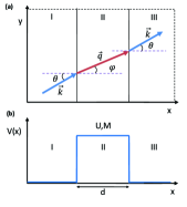
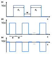
Figure 1: (Colour online) (a) Schematics of the scattering of a particle by a barrier, with $\theta$ the angle of incidence and $\phi$ that of refraction. The vectors $\vec{k}$ and $\vec{q}$ represent the wave vectors inside (II) and outside (I, III) the barrier, respectively. (b) A single potential barrier: $U$ denotes its height, $d$ its width, and $M$ the exchange field. (c) A double-barrier with inter-barrier separation $w$. (d), (e): Arrays of identical barriers and wells.

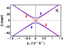
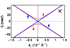
Figure 2: (Colour online) Energy spectrum of silicene in the $K$ valley (left) and $K^{\prime}$ valley (right) of the spin up (blue curve) and spin down (red dashed curve) electrons. The applied electric field is at its critical value $E_{z}=E_{c}$.

II.1 Transmission and resonances

The eigenfunctions of Eq. (1) in regions I, II, and III can be written in terms of incident and reflected waves and are matched at the interfaces between these regions. The calculation is based on the one presented in Ref. BVD, and its details are given in the appendix. If we neglect the very small ezawa1 ; ezawa3 Rashba terms , the Hamiltonian becomes block-diagonal and the eigenfunctions two-component spinors instead of the four-component spinors given in the appendix. This gives simple analytic expressions. The transmission through a single barrier reads

$$T_{\eta s_{z}}(k_{x},k_{y})=\frac{1}{1+\sin^{2}(dq_{x})\big{[}F^{2}(k_{x},q_{x},k_{y})-1\big{]}},$$ (3)

where

$$F(k_{x},q_{x},k_{y})=\frac{k_{x}^{2}\epsilon_{b}^{2}+q_{x}^{2}\epsilon_{o}^{2}+k_{y}^{2}(\epsilon_{b}-\epsilon_{o})^{2}}{2k_{x}q_{x}\epsilon_{b}\epsilon_{o}},$$ (4)

with $\epsilon_{b}=E-U-s_{z}M_{b}+\lambda_{so}+s_{z}\eta E_{z,b}e\ell$ and $\epsilon_{o}=E-s_{z}M_{o}+\lambda_{so}+s_{z}\eta E_{z,o}e\ell$. The subscripts $b$ and $o$ indicate the corresponding quantities in the barrier ($b$) and outside it ($o$). Equation (3) is more general than that of Refs. TY ; VV because the fields $E_{z}$ and $M$ are present in the entire structure whereas in Refs. TY ; VV they are present only in the barriers. It reduces to their result for $E_{z}=M=0$ outside the barrier. Notice that for $q_{x}d=n\pi$, $n$ integer, the transmission is perfect. These Fabry-Pérot resonances occur when half the wavelength of the wave inside the barrier fits $n$ times inside it.

A considerable simplification of Eq. (3) occurs at normal incidence ($k_{y}=0$):

$$T_{\eta s_{z}}(k_{x},0)=\frac{1}{1+\sin^{2}(dq_{x})(\alpha-\alpha^{-1})^{2}/4},$$ (5)

where $\alpha=k\epsilon_{b}/q\epsilon_{o}$. From this analytical result the difference with the graphene result $T=1$ is clear. Due to the SOI and the field $E_{z}$ the factor $\alpha$ differs from $1$. Setting $E_{z}=\lambda_{so}=0$, one obtains $\alpha=1$, i.e., the well-known graphene result $T=1$ no matter what the barrier width $d$ is. This unimpeded tunnelling at normal incidence, called Klein tunnelling, also takes place if the electric field attains its critical value $E_{c}$. In this case, however, only the spin-up (spin-down) electrons at the K ($K^{\prime})$ point experience the Klein effect. The origin of this partial Klein tunneling can be found in Eq. (3) when the condition $F^{2}(k_{x},q_{x},0)=1$ is satisfied.

The transmission probability through two barriers can also be calculated. The result is

$$T^{(2)}_{\eta s_{z}}(k_{x},k_{y})=\frac{1}{1+\sin^{2}(dq_{x})(F^{2}-1)4R_{\epsilon}^{2}},$$ (6)

with

$$R_{\epsilon}=\cos(wk_{x})\cos(dq_{x})+F\sin(wk_{x})\sin(dq_{x}).$$ (7)

With $w=0$ in Eq. (6) one obtains the transmission through a single barrier, cf. Eq. (2), of width $2d$. Again the function $F$ will be responsible for Klein tunnelling at normal incidence. Because both barriers are taken to have the same width, single-barrier resonances are maintained. The factor $R_{\epsilon}$, however, allows for an additional resonance pattern in the total double-barrier system.

For $n$ barriers the transmission amplitude is given by

$$t^{(n)}_{\eta s_{z}} = \big{[}e^{-ik_{x}l}(\cos(dq_{x})+iF\sin(wk_{x}))^{n}$$ (8)

$$- \Theta(n-1)e^{ik_{x}l}i^{n}\sin^{n}(dq_{x})G^{n-2}(F^{2}-1)\big{]}^{-1},$$

where $\Theta(x)$ is the Heaviside theta function; also

$$l=(n-1)w+(n-2)d,$$ (9)

$$G=\frac{\big{[}ik_{y}(\epsilon_{o}-\epsilon_{b})+k_{x}\epsilon_{b}\big{]}^{2}-q_{x}^{2}\epsilon_{o}^{2}}{2k_{x}q_{x}\epsilon_{b}\epsilon_{o}}.$$ (10)

For more than two barriers the additional resonances, that occurred in the two-barrier case, fade away but the single-barrier Fabry-Pérot resonances become sharper.

II.2 Conductance and polarizations

The spin- and valley resolved conductance is given by

$$g_{s_{z}\eta} = g_{0}\int_{-\pi/2}^{\pi/2}T_{s_{z}\eta}(\theta)\cos\theta,d\theta$$ (11)

where $g_{0}=e^{2}k_{F}L_{y}/2\pi h$, and $L_{y}$ is the length of the barrier along the $y$-direction. The total charge conductance $g_{c}$ is obtained by summing Eq. (11) over $\eta$ and $s_{z}$.

Making use of the measurable conductance, we can define the spin polarization as

$$p_{s}=\frac{(g_{\uparrow K}+g_{\uparrow K^{\prime}})-(g_{\downarrow K}+g_{\downarrow K^{\prime}})}{g_{\uparrow K}+g_{\downarrow K}+g_{\downarrow K^{\prime}}+g_{\uparrow K^{\prime}}},$$ (12)

with $p_{s}=1(-1)$ if the electrons are fully polarized in the up (down) mode. Analogously, we define the valley polarization by

$$p_{v}=\frac{(g_{\uparrow K}+g_{\downarrow K})-(g_{\uparrow K^{\prime}}+g_{\downarrow K^{\prime}})}{g_{\uparrow K}+g_{\downarrow K}+g_{\downarrow K^{\prime}}+g_{\uparrow K^{\prime}}}.$$ (13)

Here $p_{v}=\pm 1$ corresponds to a current that is localised completely in the $K$ ($K^{\prime}$) valley.

III Numerical results

We first present results for transmission, conductance, and spin and valley polarizations through one or several barriers and then those for one or several wells. The calculations are done using the four-component spinors given in the appendix and the fields $E_{z}$ and $M$ are everywhere. However, since the Rashba terms are indeed very small ezawa1 ; ezawa3 , there is no discernible difference, in the parameter ranges used, between the four-component spinor results and the analytic ones based on Eqs.(2)-(5) and (7). Accordingly, we show results for the case these terms are neglected and the fields $E_{z}$ and $M$ are inside the barriers.

III.1 Barriers

In Fig. 3 we present $(E,\theta)$ contour plots of the spin resolved transmission through one, two, and ten barriers in the 1st, 2nd, and 3rd row, respectively, at the $K$ valley. The left (right) column is for spin-up (spin-down) electrons. The electric field is chosen to be the critical field $E_{c}$ as defined above. Accordingly, the spin-down electrons have a gapless and linear energy spectrum and therefore for normal incidence ($\theta=0$) the transmission for this state is 1 due to Klein tunneling. Since the spin-up state’s spectrum still shows a gap, there are no propagating modes in the barrier if the Fermi energy is close to $U$. Thus, the transmission is suppressed in an energy region of the size of the gap around the top of the barrier.

Moving to the 2nd row of Fig. 3, for two barriers, one sees additional resonances. Remarkably they also appear in the gap indicating that they correspond to localized states in the region between the barriers. Note, however, that they disappear as we move to the 3rd row (10 barriers). This is because the additional resonances appearing for $n=2$ are due to a confinement in the total barrier structure and become highly damped for $n=10$. The only resonances that are undamped in this case are the single-barrier resonances since they are shared by all barriers. These resonances are sharper since the near-resonance evanescent modes that contribute to the transmission are suppressed because the effective length of the barrier is larger. The same mechanism also renders the gap in the transmission wider for $\theta=0$.

The shape of the Fabry-Pérot resonances in the ($E$,$\theta$) plane can be understood by applying the condition $q_{x}d=n\pi$ for the energy. The result for the simplified case where $E_{z}=M=0$ is ($r=n\pi\upsilon_{F}/Vd$)

$$E(\theta)/U=\text{sign }U\pm\big{[}1+(r^{2}-1)\cos^{2}\theta)\big{]}^{1/2}\big{/}\cos^{2}\theta$$ (14)

This relation is shown as dashed lines in Fig. 3. For the values of $n$ for which $r^{2}-1$ is small, the energy solutions become approximately independent of $\theta$, which corresponds to resonances at low energies almost independent of $\theta$. For other values of $n$ the resonant energies behave proportional to $1/\cos^{2}\theta$.

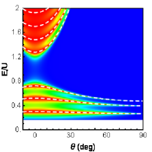
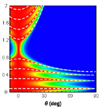
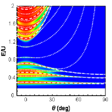
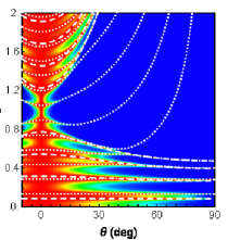
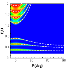
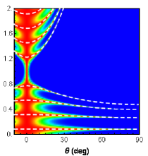
Figure 3: (Colour online) $(E,\theta)$ contour plots of the transmission probability through $1,2$, and $10$ barriers in the 1${}^{\text{st}}$, 2${}^{\text{nd}}$, and 3${}^{\text{rd}}$ row, respectively. The left (right) column is for spin-up (spin-down) electrons at the $K$ point. The dashed white curves show the resonances calculated by Eq. (14) and the dotted white curves correspond to the solutions of $R_{\epsilon}=0$ from Eq. (7). In the white region in the left column the transmission is undefined due to the lack of propagating states outside the barrier. Parameters used: $d=100$ nm, $w=50$ nm, $M=0\lambda_{so}$ , $E_{z}=E_{c}$, and $U=50$ meV.

Because experimentally one measures the conductance and not the transmission, we show in Fig. 4 the conductance as a function of the field $E_{z}$ (first row) and of the field $M$ (second row) for $1,3$, and $10$ barriers as indicated. We see that the conductance is symmetric with respect to both $E_{z}$ and $M$, it is reduced by increasing the number of barriers, and, perhaps more important, it develops a gap, i.e., it vanishes, when plotted versus $M$, for very strong fields $E_{z}$. The physical origin of the transport gap lies in the suppression of evanescent modes as $E_{z}$ increases. For one barrier this is similar to the transport gap of the conductance, plotted versus the energy at the Dirac point VV . If $E_{F}$ is fixed at the correct value, there are no propagating modes inside the barrier region. The field $M$ can then be used to shift the spectra of both spins so as to coincide with $E_{F}$. This gives rise to the observed abrupt increase in the conductance as a function of $M$. With many barriers in the system, the contribution of evanescent modes near the edges of the gap is exponentially suppressed. Therefore, the gap is widened and sharpened.

Because evanescent tunneling is suppressed with the number of barriers, the spin $p_{s}$ and valley $p_{v}$ polarizations are altered as shown in Fig. 5 versus $M$. For one barrier this is similar to the $p_{s}$ or $p_{v}$ results (versus $U/E_{F}$) of Ref. VV . Notice, though, that the $M$ ranges of near perfect $p_{s}$ and $p_{v}$ widen with the number of barriers.

In Fig. 6 we show the dependence of the conductance, spin and valley polarization on the fields $E_{z}$ and $M$. The results show that it is possible to achieve independently a strong spin and valley polarization by a proper tuning of these fields. For example, at the position marked with $\times$, the current is polarized in the $K^{\prime}$ valley ($p_{v}=-1$) but also consists only of spin-up particles ($p_{s}=1$). The use of multiple barriers makes this polarization more pronounced. The maps in Fig. 6 enable one to select the desired $p_{s}$ and $p_{v}$ by tuning the fields $E_{z}$ and $M$.

The spin and valley polarizations in Fig. 6 are shown for the Fermi level just beneath the height of the potential barrier $U$, i.e., $E_{F}\equiv E=0.8U$. In contrast, in Fig. 7 we shown them for 10 barriers in the reverse case, i.e., for $E_{F}=E=1.2U$. The results are opposite to the ones shown in Fig. 6 and show that tuning $E_{F}$ is another way of selecting the desired spin and valley polarization. Again considering the position of the $\times$ symbol, the current is $K$-valley- ($p_{v}=1$) and spin-down polarized ($p_{s}=-1$).

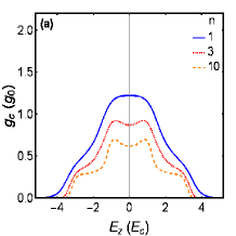
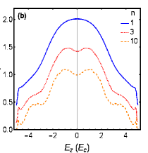
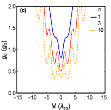
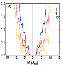
Figure 4: (Colour online) (a) and (b): conductance through $n$ barriers versus electric field $E_{z}$ for $M=\lambda_{so}$ and $M=4\lambda_{so}$ respectively. (c) and (d): Conductance versus $M$ for $E_{z}=E_{c}$ and $E_{z}=5E_{c}$, respectively. Other parameters: $d=100$ nm, $w=50$ nm, $U=50$ meV and $E=40$ meV.

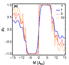
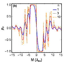
Figure 5: (Colour online) Spin (a) and valley (b) polarizations through $n$ barriers versus exchange field $M$. Parameters used: $d=100$ nm, $w=50$ nm, $E_{z}=5E_{c}$ , $E=40$ meV and $U=50$ meV

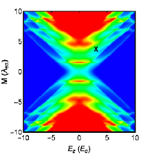
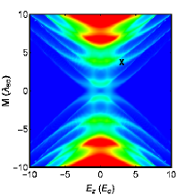
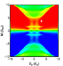
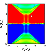
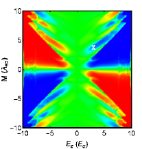
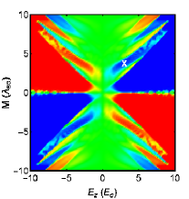
Figure 6: (Colour online) Conductance (top), spin (middle) and valley polarization (bottom) through $2$ (left column) and $10$ (right column) barriers as a function of the electric and exchange field. The unit for the conductance plots is $g_{0}$. The symbol $\times$ indicates the parameters for which the current is polarized in the $K^{\prime}$-valley and only consists of spin-up particles. Parameters used: $d=100$ nm, $w=50$ nm, $E=40$ meV and $U=50$ meV.

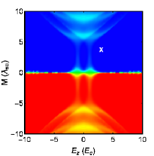
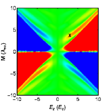
Figure 7: (Colour online) ($M,E_{z}$) contour plots of the spin (left) and valley (right) polarizations through 10 barriers for $E_{F}>U$. The position of the symbol $\times$ is the same as in Fig. 6. Parameters used: $d=100$ nm, $w=50$ nm, $E=60$ meV, and $U=50$ meV.

We can also exploit the additional degree of freedom given by the barrier separation $w$ to tune the polarization. In Fig. 8 we show a $(d,w)$ contour plot of the conductance and polarizations for $two$ barriers. As shown, increasing the barrier width $d$ has a progressively detrimental effect on the conductance. But, thanks to the periodic dependence of all these quantities at appropriate values of $d$, it is possible to realize a pure spin polarization and a valley mixed state as shown in Fig. 8.

We further explore the spin and valley polarizations by changing the magnetization $M$ of the two barriers independently at fixed barrier width $d$, as shown in Fig. 9, and by changing the width at fixed $M$, as shown in Fig. 10. In Fig. 9 $M_{1}$ and $M_{2}$ are the FM fields in the first and second barrier, respectively, and in Fig. 10 $d_{1}$ and $d_{2}$ the corresponding widths. In either figure the left panels are for the conductance, the central ones for the spin polarization, and the right panels for the valley polarization. The central panel in Fig. 10 shows a near perfect spin-up polarization for a very wide range of $d_{1}$ and $d_{2}$. This can become spin-down polarization if we reverse $M$ or change $U$. In either case we have a perfect spin filter, say, for $d_{i}\geq 7$ nm, $i=1,2$.

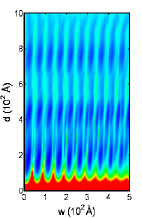
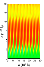
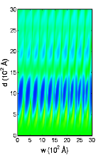
Figure 8: (Colour online) ($d,w$) contour plot of the conductance (left) through $2$ barriers, of the spin polarization (center), and of the valley polarization (right) for $M=\lambda_{so}$ , $E_{z}=5E_{c}$, $E=40$ meV and $U=50$ meV. The unit for the conductance plots is $g_{0}$.

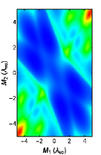
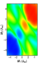
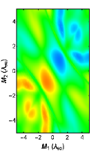
Figure 9: (Colour online) $(M_{1},M_{2})$ contour plot of the conductance (left) through $2$ barriers, of the spin polarization (center), and of the valley polarization (right). Parameters used: $E_{z}=2E_{c}$, $d_{1}=d_{2}=100$ nm, $w=50$ nm, $E=40$ meV and $U=50$ meV. The unit for the conductance plots is $g_{0}$.

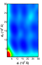
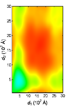
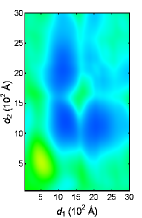
Figure 10: (Colour online) $(d_{1},d_{2})$ contour plot of the conductance (left) through $2$ barriers, of the spin polarization (center), and of the valley polarization (right). Parameters used: $E_{z}=2E_{c}$, $M_{1}=M_{2}=\lambda_{so}$, $w=50$ nm, $E=40$ meV and $U=50$ meV. The unit for the conductance plots is $g_{0}$.

III.2 Wells

Formally changing $U$ to $-U$ in Eq. (3) allows us to consider a set of wells as presented in Fig. 1(e). In Fig. 11 we show $(E,\theta)$ contour plots of the transmission in the presence of $1,2$, and $10$ wells. The left (right) column is for spin-up (spin-down) electrons. As seen, similar to the case of graphene milt , for certain angles the transmission is periodic in energy. Similar to the case of barriers, for the double well there is a new resonance pattern appearing and for a large number of wells the resonances become sharper and only those related to the single well case survive. Notice that the transmission is nearly perfect in a wider range of angles $\theta$ compared to that for barriers.

As far as the conductance is concerned, Fig. 12 shows that its overall behaviour, versus $E_{z}$ and $M$, is similar to that for barriers shown in Fig. 4. However, we don’t have a gap versus $M$, as in Fig. 4 because now the modes are always propagating. As for the spin and valley polarizations, they are about one order of magnitude smaller than those involving barriers and are not shown.

As a function of the energy, the conductance is shown in Fig. 13 for $n$ barriers on the left and for $n$ wells on the right. Notice the difference in the vertical scales and the overall reduction with increasing $n$. For $n=1$ the behaviour is similar to that of Refs. TY ; VV for silicene and Ref. milt for graphene. The reduction with increasing $n$ can be understood by the fact the conductance is mainly governed by evanescent tunneling of modes that are near resonant. This results in a smearing of the resonances and of the transmission due to Klein-tunneling and, consequently, a decrease of the conductance in the multi-barrier or multi-well system.

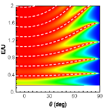
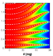
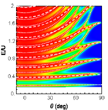
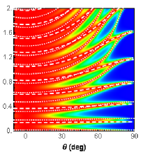
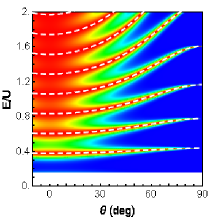
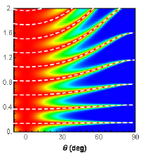
Figure 11: (Colour online) $(E,\theta)$ contour plots of the transmission through one, two, and ten wells in the 1st, 2nd, and 3rd row respectively. The left (right) column is for spin-up (spin-down) electrons. The dashed white curves show the resonances calculated by Eq. (14) and the dotted white curves correspond to the solutions of $R_{\epsilon}=0$. In the white region in the left column the transmission is undefined due to the lack of propagating states outside the barrier. Parameters used are: $d=100$ nm, $w=50$ nm, $M=0\lambda_{so}$ meV, $E_{z}=E_{c}$ and $U=-50$ meV

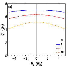
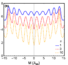
Figure 12: (colour online) Conductance over $n$ wells versus (a) the electric field for $M=\lambda_{so}$ and (b) the exchange field for $E_{z}=5E_{c}$. The other parameters are $d=100$ nm, $w=50$ nm, and $U=-50$ meV.

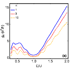
Figure 13: (Colour online) Conductance through $n$ (a) barriers and (b) wells over a length $L_{y}=100$ nm as a function of the ratio $E/U$, ($E\equiv E_{F}$). The parameters are $d=100$ nm, $w=50$ nm, $M=\lambda_{so}$, $E_{z}=E_{c}$ $|U|=50$ meV.

IV Summary and conclusions

The use of multiple barrier and well structures allows for a new approach in searching for tunable valley and spin polarizations in silicene. Our analytical results help to clearly comprehend the transmission resonances in multi-barrier and multi-well structures.

We found that a transport gap in the conductance develops not only when $U$ is varied TY ; VV but also when $M$ is. For multiple barriers this gap, as well as the spin and valley polarizations, widen with $n$ because of the suppression of nearly propagating modes. This same mechanism also sharpens the resonances found in single barriers.

The quantitative assessment of the conductance and of the polarizations, as functions of the applied electric and exchange fields, the width of the barriers or wells and their separation, suggests a selection of parameters to use in order to obtain the desired spin and valley polarizations. In this respect, one may wonder how reasonable the parameters we used are. As a matter of fact, a typical $E_{z}$ value is jang $V/6$ nm and one for $M$, though for graphene brat , is $M=3$ meV. Additionally, the use of electric field strengths up to 2.7 V/nm have been reported for bilayer graphene ExpEz . Accordingly, the range of the $E_{z}$ and $M$ values used in our calculations as well as some critical values of theirs are entirely reasonable. We also notice that all these quantities oscillate nearly periodically with the separation between barriers or wells.

Finally we showed that for wells the conductance oscillates with the exchange field and that the transport gap observed for barriers is absent.

Calculation of the transmission

The Hamiltonian for silicene with a perpendicular electric field $E_{z}$ and magnetization M at the $K$ point in the basis $\{\phi_{A}^{\uparrow},\phi_{A}^{\downarrow},\phi_{B}^{\uparrow},\phi_{B}^{\downarrow}\}$ is given by

$$H_{K}(\vec{k})=\begin{pmatrix}E_{1}(1,1)&i\lambda_{R}a\hat{k}_{-}&\upsilon_{F}\hat{k}_{-}&0\\ -ia\lambda_{R}\hat{k}_{+}&E_{1}(-1,1)&0&\upsilon_{F}\hat{k}_{-}\\ \upsilon_{F}\hat{k}_{+}&0&E_{1}(1,-1)&-ia\lambda_{R}\hat{k}_{-}\\ 0&\upsilon_{F}\hat{k}_{+}&ia\lambda_{R}\hat{k}_{+}&E_{1}(-1,-1)\end{pmatrix}$$ (15)

and at the $K^{\prime}$ point by

$$H_{K^{\prime}}(\vec{k})=\begin{pmatrix}E_{-1}(1,1)&-i\lambda_{R}a\hat{k}_{-}&\upsilon_{F}\hat{k}_{+}&0\\ ia\lambda_{R}\hat{k}_{+}&E_{-1}(-1,1)&0&\upsilon_{F}\hat{k}_{+}\\ \upsilon_{F}\hat{k}_{-}&0&E_{-1}(1,-1)&ia\lambda_{R}\hat{k}_{-}\\ 0&\upsilon_{F}\hat{k}_{-}&-ia\lambda_{R}\hat{k}_{+}&E_{-1}(-1,-1)\end{pmatrix}$$ (16)

where $a$ is the interatomic distance, $\lambda_{R}$ a very small ezawa1 ; ezawa3 SOI constant, and

$$E_{\eta}(s_{z},\tau_{z})=\eta\lambda_{so}s_{z}\tau_{z}+lE_{z}\tau_{z}+M_{z}s_{z}.$$ (17)

The wave functions $\Psi$ are given by the matrix product

$$\Psi_{j}=P_{j}E_{j}(x)C_{j}$$ (18)

which, for the $K$ point, are given by:

$$P_{1} = \begin{pmatrix}1&1&\mu&\mu\\ \zeta k_{1-}&-\zeta k_{1+}&\eta k_{2_{-}}&-\eta k_{2+}\\ \xi k_{1+}&-\xi k_{1-}&\chi k_{2+}&-\chi k_{2-}\\ \nu&\nu&1&1\end{pmatrix}\,,$$ (19)

$$E_{1}(x) = \begin{pmatrix}e^{ik_{1}x}&0&0&0\\ 0&e^{-ik_{1}x}&0&0\\ 0&0&e^{ik_{2}x}&0\\ 0&0&0&e^{-ik_{2}x}\end{pmatrix},$$ (20)

$$C_{j}=(A_{j},\quad B_{j},\quad C_{j},\quad D_{j})^{T},$$ (21)

where $T$ denotes the transpose and $k_{i\pm}=k_{i}\pm ik_{y},\,i=1,2$. Also, with $a_{\lambda}=a^{2}\lambda_{R}^{2}$ we have

$$k_{1}=[k_{F1}^{2}-k_{y}^{2}]^{1/2},\quad k_{2}=[k_{F2}^{2}-k_{y}^{2}]^{1/2},$$ (22)

$$k_{F1}=\big{[}a_{\lambda}E_{+}^{2}+\upsilon_{F}^{2}E_{-}^{2}-\Delta_{2}"\big{]}(a_{\lambda}+\upsilon_{F}^{2})^{-1/2},$$ (23)

$$k_{F2}=\big{[}a_{\lambda}E_{+}^{2}+\upsilon_{F}^{2}E_{+}^{2}+\Delta_{2}"\big{]}(a_{\lambda}+\upsilon_{F}^{2})^{-1/2},$$ (24)

$$\Delta_{2}"=2\sigma\sqrt{a_{\lambda}^{2}N^{2}+a_{\lambda}\upsilon_{F}^{2}\Omega+N^{2}\upsilon_{F}^{4}},$$ (25)

$$\sigma=sign[M(\Delta_{z}E+\lambda_{so}M)(a_{\lambda}\Delta_{z}+\upsilon_{F}^{2}M)],$$ (26)

$$\Omega=\Delta_{z}^{2}E_{+}^{2}+4\Delta_{z}E\lambda_{so}M+(E_{+}^{2}+\Delta_{z}^{2})M^{2}-M^{4},$$ (27)

where $E_{\pm}^{2}=E^{2}\pm\Delta_{z}^{2}-\lambda_{so}^{2}+M^{2}$ and $N^{2}=(\Delta_{z}E+\lambda_{so}M)^{2}$. Further,

$$\mu = \frac{ia\lambda_{R}\upsilon_{F}(\beta-\gamma)k_{F2}^{2}}{\alpha\beta\gamma-(a^{2}\lambda_{R}^{2}\gamma+\beta\upsilon_{F}^{2})k_{F2}^{2}},$$ (28)

$$\nu = \frac{-ia\lambda_{R}\upsilon_{F}(\beta-\gamma)k_{F1}^{2}}{\delta\beta\gamma-(a^{2}\lambda_{R}^{2}\beta+\upsilon_{F}^{2}\gamma)k_{F1}^{2}},$$ (29)

$$\zeta = \frac{ia\lambda_{R}+\upsilon_{F}\nu}{\beta},\,\,\eta=\frac{ia\lambda_{R}\mu+\upsilon_{F}}{\beta},$$ (30)

$$\xi = \frac{ia\lambda_{R}\nu+\upsilon_{F}}{\gamma},\,\,\chi=\frac{ia\lambda_{R}+\upsilon_{F}\mu}{\gamma}.$$ (31)

$$\alpha = \left(E-lE_{z}-\lambda_{so}-M\right)$$

$$\beta = \left(E-lE_{z}+\lambda_{so}+M\right)$$

$$\gamma = \left(E+lE_{z}+\lambda_{so}-M\right)$$

$$\delta = \left(E+lE_{z}-\lambda_{so}+M\right)$$ (32)

and at the $K^{\prime}$ point:

$$P_{1}^{\prime} = \begin{pmatrix}\eta^{\prime}k_{1+}^{\prime}&-\eta^{\prime}k_{1-}^{\prime}&\zeta^{\prime}k_{2+}^{\prime}&-\zeta^{\prime}k_{2-}^{\prime}\\ 1&1&\nu^{\prime}&\nu^{\prime}\\ \mu^{\prime}&\mu^{\prime}&1&1\\ \chi^{\prime}k_{1-}^{\prime}&-\chi^{\prime}k_{1+}^{\prime}&\xi^{\prime}k_{2-}^{\prime}&-\xi^{\prime}k_{2+}^{\prime}\end{pmatrix}$$ (33)

where $k_{i\pm}^{\prime}=k_{i}^{\prime}\pm ik_{y},\,i=1,2$. The matrix $E_{1}^{\prime}(x)$ is obtained from $E_{1}(x)$ by changing $k_{i}$ to $k_{i}^{\prime}$. Also, $k_{i}^{\prime}$ and $k_{Fi}^{\prime}$ are obtained from $k_{i}$ and $k_{Fi}$ by the same change followed by $\Delta"_{2}\to\Delta_{2}"^{\prime}$.

$$\mu^{\prime} = \frac{ia\lambda_{R}\upsilon_{F}(\alpha^{\prime}-\delta^{\prime})k_{F2}^{2}}{\beta^{\prime}\alpha^{\prime}\delta^{\prime}-(a^{2}\lambda_{R}^{2}\delta^{\prime}+\upsilon_{F}^{2}\alpha^{\prime})k_{F2}^{2}}$$ (34)

$$\nu^{\prime} = \frac{-ia\lambda_{R}\upsilon_{F}(\alpha^{\prime}-\delta^{\prime})k_{F1}^{2}}{\gamma^{\prime}\alpha^{\prime}\delta^{\prime}-(a^{2}\lambda_{R}^{2}\alpha^{\prime}+\upsilon_{F}^{2}\delta^{\prime})k_{F1}^{2}}$$ (35)

$$\zeta^{\prime} = \frac{ia\lambda_{R}+\upsilon_{F}\nu^{\prime}}{\alpha^{\prime}},\,\,\eta^{\prime}=\frac{ia\lambda_{R}\mu^{\prime}+\upsilon_{F}}{\alpha^{\prime}},$$ (36)

$$\xi^{\prime} = \frac{ia\lambda_{R}\nu^{\prime}+\upsilon_{F}}{\delta^{\prime}},\,\,\chi^{\prime}=\frac{ia\lambda_{R}+\upsilon_{F}\mu^{\prime}}{\delta^{\prime}}.$$ (37)

$$\alpha = \left(E-lE_{z}-\lambda_{so}-M\right)$$

$$\beta = \left(E-lE_{z}+\lambda_{so}+M\right)$$

$$\gamma = \left(E+lE_{z}+\lambda_{so}-M\right)$$

$$\delta = \left(E+lE_{z}-\lambda_{so}+M\right)$$ (38)

$$\alpha^{\prime} = \left(E-lE_{z}+\lambda_{so}-M\right)$$

$$\beta^{\prime} = \left(E-lE_{z}-\lambda_{so}+M\right)$$

$$\gamma^{\prime} = \left(E+lE_{z}-\lambda_{so}-M\right)$$

$$\delta^{\prime} = \left(E+lE_{z}+\lambda_{so}+M\right)$$ (39)

To calculate the transmission through an arbitrary number of barriers n, we exploit the following property of the transfer matrix through a single barrier at $x=x_{0}$:

$$M(x_{0})=E_{1}^{-1}(x_{0})P_{1}^{-1}P_{2}E_{2}(x_{0})E_{2}^{-1}(x_{0}+d_{2})$$ (40)

$$\times P_{2}^{-1}P_{1}E_{1}(x_{0}+d_{2})=E_{1}^{-1}(x_{0})M(0)E_{1}(x_{0})$$

Then the resulting transfer matrix becomes

$$M_{n} = M(0)M(d)M(2d)...M((n-1)d)$$ (41)

$$= M(0)E_{1}^{-1}(d)M(0)E_{1}(d)E_{1}^{-1}(2d)M(0)E_{1}(2d)$$

$$...E_{1}^{-1}((n-1)d)M(0)E_{1}((n-1)d)$$

$$= M(0)E_{1}^{-1}(d)M(0)E_{1}^{-1}(d)M(0)E_{1}^{-1}(d)$$

$$...E_{1}^{-1}(d)M(0)E_{1}((n-1)d)$$

$$= M(0)[E_{1}^{-1}(d)M(0)]^{n-1}E_{1}((n-1)d)$$

The transmission amplitudes $t_{\eta s_{z}}^{(n)}$ are found by solving the system of equations

$$\Big{(}1\,\,,r_{\uparrow}^{\uparrow}\,\,,0\,\,,r_{\downarrow}^{\uparrow}\Big{)}^{T}=m\Big{(}t_{\uparrow}^{\uparrow}\,\,,0\,\,,t_{\downarrow}^{\uparrow}\,\,,0\Big{)}^{T}$$ (42)

where m is the total transfer matrix of the barrier structure and $T$ denotes the transpose of the row vectors. Then the transmission is given by $T=|t_{\eta s_{z}}^{(n)}|^{2}$.

All the results so far involve the four-component spinors (17). If we neglect the very small ezawa1 ; ezawa3 constant $\lambda_{R}$, the Hamiltonian (1) becomes block-diagonal and the eigenfunctions two-component spinors. This gives the simple analytic expressions (2), (4), (5).

References

- (1) G. G. Guzmán-Verri and L. C. Lew Yan Voon, Phys. Rev. B 76, 075131 (2007); S. Lebègue and O. Eriksson, Phys. Rev. B 79, 115409 (2009).
- (2) P. Vogt, P. De Padova, C. Quaresima, J. Avila, E. Frantzeskakis, M. C. Asensio, A. Resta, B. Ealet, and G. Le Lay, Phys. Rev. Lett. 108, 155501 (2012); A. Fleurence, R. Friedlein, T. Ozaki, H. Kawai, Y. Wang, and Y. Yamada-Takamura, ibid. 108, 245501 (2012).
- (3) D. Chiappe, E. Scalise, E. Cinquanta, C. Grazianetti, B. v. Broek, M. Fanciulli, M. Houssa, and A. Molle, Adv. Mater. 26, 2096 (2014).
- (4) L. Chen, C.-C. Liu, B. Feng, X. et al, Phys. Rev. Lett. 109, 056804(2012).
- (5) L. Meng, Y.Wang, L. Zhang, et al, Nano. Lett. 13, 685 (2013).
- (6) Z. Ni, Q. Liu, K. Tang, J. Zheng, J. Zhou, R. Qin, Z. Gao, D. Yu, and J. Lu, Nano Lett. 12, 113 (2012); Y. Cai, C.-P. Chuu, C. M. Wei, and M. Y. Chou, Phys. Rev. B 88, 245408 (2013); M. Neek-Amal, A. Sadeghi, G. R. Berdiyorov, and F. M. Peeters, Appl. Phys. Lett. 103, 261904 (2013).
- (7) C.-C. Liu, W. Feng, and Y. Yao, Phys. Rev. Lett. 107, 076802 (2011).
- (8) N. D. Drummond, V. Zólyomi, and V. I. F’alko, Phys. Rev. B 85, 075423 (2012).
- (9) M. Ezawa, New. J. Phys. 14, 033003 (2012).
- (10) A. Dyrdał and J. Barnas, Phys. Stat. Sol. RRL 6, 340 (2012).
- (11) M. Tahir, A. Manchon, K. Sabeeh, and U. Schwingenschlögl, Appl. Phys. Lett. 102, 162412 (2013).
- (12) C. J. Tabert and E. J. Nicol, Phys. Rev. B 87, 235426 (2013).
- (13) M. Ezawa, Phys. Rev. Lett. 109, 055502 (2012).
- (14) L. Stille, C. J. Tabert, and E. J. Nicol, Phys. Rev. B 86, 195405 (2012).
- (15) A. Kara, H. Enriquez, A. P. Seitsonen, L.C. Lew Yan Voon, S. Vizzini, B. Aufray, and H. Oughaddoub, Surf. Sci. 67, 1 (2012).
- (16) C.-C. Liu, H. Jiang, and Y. Yao, Phys. Rev. B 84, 195430 (2011).
- (17) B. Huang, D. J. Monsma, and I. Appelbaum, Phys. Rev. Lett. 99, 177209 (2007).
- (18) Y. Wang, J. Zheng, Z. Ni, R. Fei, Q. Liu, R. Quhe, C. Xu, J. Zhou, Z. Gao, and J. Lu, Nano 07, 1250037 (2012).
- (19) S. Sanvito, Chem. Soc. Rev. 40, 3336 (2011).
- (20) N. Tombros, C. Jozsa, M. Popinciuc, H. T. Jonkman, and B. J. van Wees, Nature 448, 571 (2007).
- (21) L.Tao, E. Cinquanta, D. Chiappe, C. Grazianetti, M. Fanciulli, M. Dubey, A. Molle and D. Akinwande Nature Nanotechnology 10, 227 (2015)
- (22) H. Haugen, D. Huertas-Hernando, and A. Brataas, Phys. Rev. B 77, 115406 (2008).
- (23) J. Milton Pereira, Jr., P. Vasilopoulos, and F. M. Peeters, Appl. Phys. Lett. 90, 132122 (2007).
- (24) S. Mondal, D. Sen, K. Sengupta, and R. Shankar, Phys. Rev. Lett. 104, 046403 (2010).
- (25) T. Yokoyama, Phys. Rev. B 87, 241409(R) (2013).
- (26) B. Soodchomshom, J. Appl. Phys. 115, 023706 (2014).
- (27) V. Vargiamidis and P. Vasilopoulos, Appl. Phys. Lett. 105, 223105 (2014); J. Appl. Phys. 117, 094305 (2015).
- (28) B. Van Duppen, S. H. R. Sena, and F. M. Peeters, Phys. Rev. B 87, 195439 (2013)
- (29) M. Barbier, F. M. Peeters, P. Vasilopoulos, and J. Milton Pereira, Jr., Phys. Rev. B 77, 1 (2008).
- (30) J. Milton Pereira, Jr., P. Vasilopoulos, and F. M. Peeters, Appl. Phys. Lett. 90, 132122 (2007).
- (31) H. Min, J.E. Hill, N.A. Sinitsyn, B.R. Sahu, L. Kleinman and A.H. MacDonald, Phys. Rev. B 74, 165310 (2006).
- (32) K. F. Mak, C.H. Lui, J. Shan and T. F. Heinz, Phys. Rev. Lett. 102, 256405 (2009)