Limb-darkening coefficients from line-blanketed non-LTE hot-star model atmospheres

Abstract

We present grids of limb-darkening coefficients computed from non-LTE, line-blanketed tlusty model atmospheres, covering effective-temperature and surface-gravity ranges of 15–55 kK and 4.75 dex (cgs) down to the effective Eddington limit, at 2$\times$, 1$\times$, 0.5$\times$ (LMC), 0.2$\times$ (SMC), and 0.1$\times$ solar. Results are given for the Bessell UBVRI_CJKHL, Sloan ugriz, Strömgren ubvy, WFCAM ZYJHK, Hipparcos, Kepler, and Tycho passbands, in each case characterized by several different limb-darkening ‘laws’. We examine the sensitivity of limb darkening to temperature, gravity, metallicity, microturbulent velocity, and wavelength, and make a comparison with LTE models. The dependence on metallicity is very weak, but limb darkening is a moderately strong function of $\log{g}$ in this temperature regime.

1 Introduction

An accurate description of limb darkening is essential to any investigation involving the direct or indirect spatial resolution of a stellar surface. Modelling of eclipsing-binary light-curves has been a major application historically, but studies of exoplanetary transits and microlensing events, and interferometric observations of stellar surfaces, have similar requirements.

The advent of good-quality line-blanketed LTE model atmospheres (particularly from Kurucz’s Atlas codes; Kurucz 1979) made it possible to generate large grids of synthetic spectra, and associated limb-darkening coefficients, for wide ranges of stellar parameters (e.g., Wade & Rucinski 1985; Claret 2000; Howarth 2011a, and references therein). Results for non-LTE models are fewer, for reasons of computational complexity and expense, and available grids extend only to $T_{\rm eff}\lesssim$10 kK (Claret & Hauschildt 2003; Claret et al. 2012, 2013).

Here we report results from line-blanketed non-LTE models for the OB-star regime. These may be of particular interest in the study of extragalactic eclipsing-binary systems, where hot, luminous stars present good opportunities for direct distance-scale determinations, in addition to measurements of basic stellar parameters (e.g., Harries et al. 2003; Hilditch et al. 2005; Bonanos et al. 2009; North et al. 2010). They should also have applicability in accurate photometric modelling of hot stars that depart from spherical symmetry, through rapid rotation (as in the case of Be stars; e.g., Townsend et al. 2004), pulsation, or surface inhomogeneities (e.g., Ramiaramanantsoa et al. 2014; Buysschaert et al. 2015).

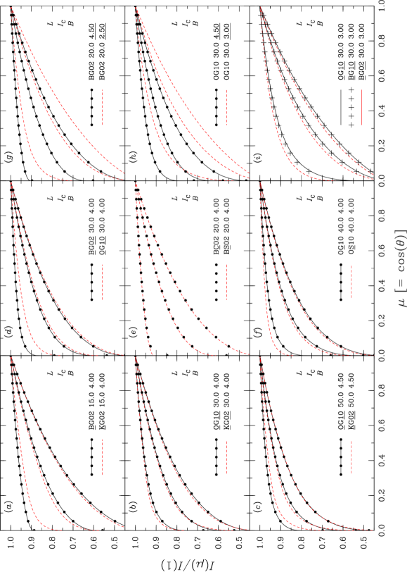
Figure 1: Representative intensity distributions to illustrate the sensitivity of computed limb darkening to temperature (compare, e.g., panels $a$–$c$), gravity (panels $g$, $h$), microturbulence ($d$, $i$), abundance ($e$, $f$), and wavelength (Johnson B, I_C, and L bands throughout). Models are identified by source (B, O are non-LTE tlusty Bstar2006 and Ostar2002 results; K denotes Atlas [‘Kurucz’] LTE calculations, from Howarth 2011a), microturbulence (2 or 10 $\mbox{km}\;\mbox{s}^{-1}$), abundance (C, G, S for $Z/Z_{\odot}=2,1,0.2$), effective temperature (in kK), and $\log{g}$ (cgs). Continuous and dashed curves are parametrized (4-coefficient) characterizations, with dots (and ‘+’ symbols) showing individual computed $I(\mu)$ values. [The centre panel does correctly display results of two different, but almost indistinguishable, models.] See $\S$3 for discussion.

2 Method

2.1 Models

Our calculations make use of line-blanketed tlusty models (Hubeny & Lanz, 1995); these assume plane-parallel, hydrostatic atmospheres, relaxing the approximation of local thermodynamic equilibrium. Two extensive grids of structures are available, based on these models: Ostar2002 (Lanz & Hubeny 2003; 27.5–55.0 kK) and Bstar2006 (Lanz & Hubeny 2007; 15.0–30.0 kK), each extending over a range of surface gravities from 4.75 dex (cgs) to the effective Eddington limit, at several metallicities.

Table 1: Summary of models; sampling in gravity is at steps of 0.25 dex. Metallicity codings are identified in columns 7–11 (e.g., the L grid corresponds to $Z/Z_{\odot}=0.5$); $\xi$ is the microturbulence; $N$ is the number of models. The high-$\xi$ models summarized in the final row of the Table are intended to correspond to B supergiants, and do not extend to main-sequence gravities (cf. Lanz & Hubeny 2007); in view of the weak sensitivity of results to metallicity, we computed only solar-metallicity LDCs for these models.

Grid	$T_{\rm eff}$	$\log{g}$ (min)		(max)	$\xi$	$Z/Z_{\odot}$ coding					$N$
	(kK)	[$T_{\rm eff}$(lo)]	$T_{\rm eff}$(hi)]		($\mbox{km}\;\mbox{s}^{-1}$)	——————————–
OStar02	27.5–55.0 @ 2.5	3.00	4.00	4.75	10	2	1	0.5	0.2	0.1	345
BStar06	15.0–30.0 @ 1.0	1.75	3.00	4.75	2	C	G	L	S	T	817
BStar06	15.0–30.0 @ 1.0	1.75	3.00	3.00	10		G				49

We computed emergent intensities from the atmospheric structures with moderately dense wavelength sampling (median interval $\sim$0.4Å) at 20 angles, approximately equally spaced over the range 0.001–1 in $\mu\equiv\cos\theta$, where $\theta$ is the emergent angle measured from the surface normal. The calculations were made using Hubeny’s synspec code, with the accompanying line lists augmented with data from Kurucz’s gfall compilation, to extend coverage of (near-)IR wavelengths.

Results were used to generate broad-band specific intensities appropriate for photon-counting detectors (such as CCDs),

$$I_{i}(\mu)=\frac{\int_{\lambda}I_{\lambda}(\mu)\;\phi_{i}(\lambda)\;\lambda\;\text{d}\lambda}{\int_{\lambda}\phi_{i}(\lambda)\;\lambda\;\text{d}\lambda}$$

where $\phi_{i}(\lambda)$ is the response function for passband $i$. We employed the response functions adopted by Howarth (2011a) for the Bessell UBVRI_CJKHL, Sloan ugriz, Strömgren ubvy, WFCAM ZYJHK, Hipparcos, Kepler, and Tycho passbands.

Figure 2: Linear (one-parameter) limb-darkening coefficients for selected models, to illustrate $\log{g}$, $\xi$, and metallicity dependences. Results are labelled by Johnson passband and $\log{g}$  (additional results are available at intermediate gravities); ‘G’ and ‘S’ models have $Z/Z_{\odot}=1$ and 0.2, respectively; ‘K’ identifies LTE (Kurucz) results from Howarth (2011a). $B$-band results for B-star models at $\log{g}=2.5$ and 3.0 are shown for both $\xi=2$ & 10 $\mbox{km}\;\mbox{s}^{-1}$(‘normal’ and ‘supergiant’ values).

2.2 Characterization

Particularly for photometric applications, limb darkening is, in practice, conveniently characterized by ad hoc analytical ‘laws’ representing the specific intensities (or monochromatic radiances), thereby reducing the data description to a small set of limb-darkening coefficients (LDCs).

While numerous limb-darkening laws have been proposed (cf., e.g., Claret 2000; Howarth 2011a), current observations (particularly of exoplanetary transits) are generally capable of usefully constraining only one- or two-parameter forms. The analytical solution for a model atmosphere in which the source function is linear in optical depth is

$${I_{\lambda}(\mu)}={I_{\lambda}(1)}\left[{1-u_{\lambda}(1-\mu)}\right]$$ (1)

and use of this linear limb-darkening law persists in the context of light-curve modelling, although it often gives a rather poor representation of model-atmosphere emergent intensities. A quadratic law,

$${I_{\lambda}(\mu)}={I_{\lambda}(1)}\left[{1-u_{1,\lambda}(1-\mu)-u_{2,\lambda}(1-\mu)^{2}}\right]$$ (2)

offers greater flexibility, and two coefficients represent the practical limit for empirical determinations of LDCs (within limits; cf., e.g., Howarth 2011b; Müller et al. 2013). The most accurate algebraic representation of model-atmosphere results in routine use is the 4-parameter law introduced by Claret (2000),

$${I_{\lambda}(\mu)}={I_{\lambda}(1)}\left[{1-\sum\limits_{k=1}^{4}a_{k,\lambda}(1-\mu^{k/2})}\right],$$ (3)

which is able to fit intensity profiles across a wide parameter space with good accuracy.

2.3 Results

The 1 211 models for which we have computed emergent intensities are summarized in Table 1. For each model we calculated LDCs for each ‘law’ (eqtns. 1–3) by least-squares fits of the given functions to $I_{i}(\mu)$ over the range $0.05\leq\mu\leq 1.00$, with and without $I_{i}(1)$ as a free parameter in the fit. We also computed flux-conserving least-squares coefficients for the linear and quadratic laws (following Howarth 2011b). Results are presented on-line (q.v. Appendix A).

3 Discussion and Conclusions

Figure 1 shows the general form of the limb darkening at representative values of temperature, gravity, abundance, and wavelength; and illustrates the sensitivity to technical details of the different models (Ostar2002, Bstar2006, and line-blanketed LTE models from Howarth 2011a). These aspects are reviewed across a broader parameter space, but in a coarser manner, in Fig. 2, which shows the linear limb-darkening coefficient for a range of models (eqtn. 1, $I(1)$ fixed; see also Fig. 1 of Howarth 2011b).

As well as the obvious dependences on temperature and passband (generally, smaller limb-darkening at longer wavelengths), there is a fairly strong dependence on gravity in the OB-star regime (Fig. 2; Fig. 1, panels g, h), although the sensitivity to metallicity is rather weak (panels e, f).

Differences in limb-darkening between Kurucz (LTE) and tlusty (non-LTE) models turn out to be reasonably small (Fig. 1, panels $a$–$c$). As expected, the Bstar2006 models at $\xi=10$ $\mbox{km}\;\mbox{s}^{-1}$ are in excellent agreement with their Ostar2002 counterparts in their limited overlap range, and both show only small differences from the $\xi=2$ $\mbox{km}\;\mbox{s}^{-1}$ B-star models (Fig. 1i).

Finally, it should be borne in mind that the LDCs presented here are all based on hydrostatic, plane-parallel model structures. Real O stars, and B supergiants (at least), have substantial stellar winds, which raises the question of the applicability of our results. Lanz & Hubeny (2003) address this issue at some length, and conclude that tlusty models give a satisfactory representation of most spectral lines in the UV–IR regime (a conclusion that applies a fortiori to the continuum), and that line blanketing is the more important consideration. We therefore expect our broad-band LDCs to provide a reasonable description of nature, other than when the continuum forms in dynamical layers or where spherical extension is significant (e.g., in Luminous Blue Variables). These circumstances probably occur only outside the $\log{g}$ domain covered by the grids.

Appendix A On-line material

Results are given in two summary files (one for linear and quadratic forms and one for 4-coefficient fits), and for individual models, identifiable by file name; e.g., the file BG20000g425v02.LDC is from the Bstar06, G-abundance (‘Galactic’, $Z/Z_{\odot}=1$) grid, for $T_{\rm eff}=20$ kK, $\log{g}=4.25$, microturbulence $\xi=2$ $\mbox{km}\;\mbox{s}^{-1}$. Each individual model file contains a series of blocks giving results for different passbands; for example, BG20000g425v02.LDC starts

#-------------------------------------------------------------------------------------------------------------------------
# Bessell-UX          3598.5  5.99074E+08  2.15116E+08
  linear - 1    +1.00000E+00 +3.82029E-01                                            +2.463E-02 -6.659E-02  0.05    +1.557
  linear - 2    +1.02778E+00 +4.24870E-01                                            +1.995E-02 -5.383E-02  0.05    +0.034
  lin - FCLS    +1.02822E+00 +4.13609E-01                                            +1.996E-02 -5.387E-02  0.05     0.000
  quad - 2      +1.00000E+00 +2.16789E-01 +2.26667E-01                               +7.099E-03 -1.995E-02  0.05    -0.395
  quad - 3      +9.91711E-01 +1.82744E-01 +2.55834E-01                               +6.406E-03 +1.776E-02  0.05    -0.192
  quad - FCLS   +9.89536E-01 +1.84220E-01 +2.56568E-01                               +6.584E-03 -1.776E-02  0.05     0.000
  4-coeff       +1.00000E+00 +5.16742E-01 +5.48940E-02 -1.82686E-02 -2.91968E-03     +1.815E-05 +5.219E-05  0.11    -0.134
  1+4-coeff     +9.99981E-01 +5.17614E-01 +5.22650E-02 -1.50032E-02 -4.34753E-03     +1.729E-05 +4.932E-05  0.11    -0.133
#-------------------------------------------------------------------------------------------------------------------------
# Bessell-BX          4376.9  4.24681E+08  1.51335E+08
  linear - 1    +1.00000E+00 +3.73773E-01                                            +3.170E-02 -8.671E-02  0.05    +1.997
  linear - 2    +1.03522E+00 +4.28079E-01                                            +2.587E-02 -7.053E-02  0.05    +0.082
  ...

The first line lists

• the passband identifier (here Bessell’s characterizations of the Johnson U and B passbands used in computing $U-B$ colours);

• the effective wavelength (in Å);

• the broad-band physical flux $F_{\lambda}$ ($=4\pi H_{\lambda}$, in erg cm^-2 s^-1 Å^-1);

• the broad-band surface-normal intensity $I_{\lambda}(1)$ (in erg cm^-2 s^-1 Å^-1 sr^-1)

(multiply values by $10^{-2}$ to obtain results in units of J m^-2 s^-1 nm^-1). Subsequent lines list coefficients for the limb-darkening laws discussed in Section 2.2; ‘FCLS’ indicates values obtained by flux-conserving least squares. The first value is $\hat{I}_{\lambda}(1)/I_{\lambda}(1)$, the ratio of the fitted surface-normal intensity to the model-atmosphere value, followed by the set of limb-darkening coefficients.

The last four columns are indicators of the fit quality, being the r.m.s. and maximum O$-$C values of $I_{\lambda}(\mu)/I_{\lambda}(1)$ (where ‘O’ and ‘C’ refer to model-atmosphere and analytical-fit values); the value of $\mu$ for which the absolute value of the mismatch is greatest; and the percentage error in the flux obtained by integrating the analytical represention of the intensity to obtain the first moment of the radiation field (Eddington flux, $H_{\lambda}=F_{\lambda}/4\pi$).

The summary files extract and compile the LDC information in a format intended to be self-explanatory, and amenable to processing by simple text-manipulation tools (e.g., UNIX grep, awk, and cut commands). The Summary1.LDC file of linear and quadratic coefficients, for example, begins

# Source file    filter         I(1)     ------- linear 1 --------   +++++++ linear 2 ++++++++   ------- lin FCLS --------   +++++++++++++++ quad 2 +++++++++++
BC15000g175v02 Bessell-UX   1.36727E+08  +1.00000E+00 +5.46138E-01   +1.02181E+00 +5.79776E-01   +1.02255E+00 +5.67667E-01   +1.00000E+00 +4.20039E-01 +1.72...
BC15000g175v02 Bessell-BX   8.86990E+07  +1.00000E+00 +5.58679E-01   +1.02552E+00 +5.98034E-01   +1.02663E+00 +5.83534E-01   +1.00000E+00 +4.14861E-01 +1.97...
BC15000g175v02 Bessell-B    8.98503E+07  +1.00000E+00 +5.59268E-01   +1.02541E+00 +5.98454E-01   +1.02651E+00 +5.84003E-01   +1.00000E+00 +4.16113E-01 +1.96...
BC15000g175v02 Bessell-V    4.60602E+07  +1.00000E+00 +5.21743E-01   +1.03041E+00 +5.68644E-01   +1.03177E+00 +5.52366E-01   +1.00000E+00 +3.47071E-01 +2.39...
BC15000g175v02 Bessell-R    2.61041E+07  +1.00000E+00 +4.86751E-01   +1.03291E+00 +5.37504E-01   +1.03432E+00 +5.20945E-01   +1.00000E+00 +2.94742E-01 +2.63...
BC15000g175v02 Bessell-I    1.29020E+07  +1.00000E+00 +4.38498E-01   +1.03460E+00 +4.91859E-01   +1.03593E+00 +4.76000E-01   +1.00000E+00 +2.33205E-01 +2.81...
...

The Summary2.LDC file has corresponding results for the coefficients in eqtn. 3.

All files are intended to be available through CDS, and are presently available at ftp://ftp.star.ucl.ac.uk/idh/LDC/.

References

- Bonanos et al. (2009) Bonanos A. Z., et al., 2009, AJ, 138, 1003
- Buysschaert et al. (2015) Buysschaert B., et al., 2015, MNRAS, 453, 89
- Claret (2000) Claret A., 2000, A&A, 363, 1081
- Claret & Hauschildt (2003) Claret A., Hauschildt P. H., 2003, A&A, 412, 241
- Claret et al. (2012) Claret A., Hauschildt P. H., Witte S., 2012, A&A, 546, A14
- Claret et al. (2013) Claret A., Hauschildt P. H., Witte S., 2013, A&A, 552, A16
- Harries et al. (2003) Harries T. J., Hilditch R. W., Howarth I. D., 2003, MNRAS, 339, 157
- Hilditch et al. (2005) Hilditch R. W., Howarth I. D., Harries T. J., 2005, MNRAS, 357, 304
- Howarth (2011a) Howarth I. D., 2011a, MNRAS, 413, 1515
- Howarth (2011b) Howarth I. D., 2011b, MNRAS, 418, 1165
- Hubeny & Lanz (1995) Hubeny I., Lanz T., 1995, ApJ, 439, 875
- Kurucz (1979) Kurucz R. L., 1979, ApJS, 40, 1
- Lanz & Hubeny (2003) Lanz T., Hubeny I., 2003, ApJS, 146, 417 (erratum in 147, 225)
- Lanz & Hubeny (2007) Lanz T., Hubeny I., 2007, ApJS, 169, 83
- Müller et al. (2013) Müller H. M., Huber K. F., Czesla S., Wolter U., Schmitt J. H. M. M., 2013, A&A, 560, A112
- North et al. (2010) North P., Gauderon R., Barblan F., Royer F., 2010, A&A, 520, A74 (corrigendum in 540, C1)
- Ramiaramanantsoa et al. (2014) Ramiaramanantsoa T., et al., 2014, MNRAS, 441, 910
- Townsend et al. (2004) Townsend R. H. D., Owocki S. P., Howarth I. D., 2004, MNRAS, 350, 189
- Wade & Rucinski (1985) Wade R. A., Rucinski S. M., 1985, A&AS, 60, 471