Facial Expression Recognition Using Sparse Gaussian Conditional Random Field

Abstract

The analysis of expression and facial Action Units (AUs) detection are very important tasks in fields of computer vision and Human Computer Interaction (HCI) due to the wide range of applications in human life. Many works has been done during the past few years which has their own advantages and disadvantages. In this work we present a new model based on Gaussian Conditional Random Field. We solve our objective problem using ADMM and we show how well the proposed model works. We train and test our work on two facial expression datasets, CK+ and RU-FACS. Experimental evaluation shows that our proposed approach outperform state of the art expression recognition.

I Introduction

Over the past few years the problem of temporal classification and recognition has gained significant attention among researchers in many fields such as speech recognition, human expression classification, event detection and etc. Generally in temporal analysis the goal is to find a mapping function from the stream of observation sequences to the set of corresponding outputs. There are many algorithms that tackle this problem: in [8], the authors tackled speech recognition problem by using Hidden Markov Model (HMM). HMM is a well known classifier that by modeling the joint probability of inputs $\mathbf{x}$, and outputs $\mathbf{y}$ conditioned on a set of latent state variable learns a temporal transition. Although HMM is widely used and has been reported to work well in similar applications, there are pitfalls in using it. One of the main problems is that HMM predicts a joint probability distribution between inputs and outputs. To define a joint probability distribution between observations and labels, HMM needs to model distribution of $p(\mathbf{x})$ which can include complex dependencies. Modeling these dependencies in the input make it complex, however disregarding it reduces performance.

The solution to this problem is to instead of modeling joint probability distribution, directly model the conditional distribution $p(\mathbf{x}|\mathbf{y})$. This approach is exactly the conditional random field [6]. The conditional random field is a graphical model that maximizes the conditional probability distribution between inputs and outputs. This assumption makes CRF to have much more rich feature observation than HMM. However CRF plays an important role in many computer vision applications but in general, parameter learning and inference are very complex and time consuming because of nonlinearity and non-convexity of CRF. In [15, 9] sampling algorithms for parameters learning are used, but unfortunately, sampling algorithms are slow to convergence.

Gaussian Markov random field is the ordinary MRF model where variables are jointly Gaussian. Gaussian models are very popular in many fields of studies because of the inference in Gaussian models can be easy. Typically, the key success with Gaussian MRF as indicated in [11, 13] is the neighboring functions that are dependent on the input signal. This dependency among input signals makes GMRF to be a conditional model and can be called Gaussian Conditional Random Field (GCRF).

In this paper we introduce a model based on GCRF and show how the parameters of this model can be efficiently learned. The model we propose is based on ADMM model [3]. The rest of this paper is organized as follow: in section 2 we are going to introduce an introduction about GCRF, in section 3 our proposed model is presented and in section 4 and 5 our experimental results and conclusion are introduced respectively.

II Gaussian Conditional Random Field

In this section we are going to present an introduction about GCRF. A GCRF model can be formalized as follow:

$$p(\mathbf{y}|\mathbf{x};\Theta,\Lambda)=\frac{1}{Z(\mathbf{x})}\exp\{-\mathbf{y}^{T}\Lambda\mathbf{y}-2\mathbf{x}^{T}\Theta\mathbf{y}\}$$ (1)

where in this equation $\mathbf{x}\in\Re^{n}$is the sequence of observation inputs and $\mathbf{y}\in\Re^{p}$ is the sequence of corresponding outputs. In this equation $\Lambda$ is a parameter which model conditional dependency among $\mathbf{y}$ and $\Theta$ maps the input to output. The partition function is given by:

$$\frac{1}{Z(\mathbf{x})}=c|\Lambda|\exp\{-\mathbf{x}^{T}\Theta\Lambda^{-1}\mathbf{x}\}$$ (2)

In this model the maximum likelihood is given by getting negative log of Eq.1 and Eq.2 and is defined as follow:

$$f(\Lambda,\Theta)=-\log{|\Lambda|}+\text{tr}\{S_{yy}\Lambda+2S_{yx}\Theta+\Lambda^{-1}\Theta^{T}S_{xx}\Theta\}$$ (3)

where in this equation, terms $S$ are the empirical covariances and are:

$$S_{yy}=\frac{1}{m}\mathbf{y}^{T}\mathbf{y},S_{yx}=\frac{1}{m}\mathbf{y}^{T}\mathbf{x},S_{xx}=\frac{1}{m}\mathbf{x}^{T}\mathbf{x}$$ (4)

As indicated in [13] this equation is a convex problem and solution to this problem can be done by getting gradient with respect to parameters and using steepest descent method to find the parameters which maximize Eq.4. Unfortunately using steepest descent method is very computational and it needs many numbers of iterations for convergence. In this paper we are going to present a new method based on ADMM and show how fast we can learn parameters from the model.

III Proposed Method

As can be seen from the previous section, the main problem of GCRF is complexity and time consumption. In this section we are going to introduce our proposed method based on ADMM model after an introduction about ADMM.

III-A Alternating Direction Method of Multipliers

ADMM which first introduced by [3] is a robust and fast optimization method. Consider the optimization problem such as:

$$\min_{\mathbf{x},\mathbf{z}}\quad f(\mathbf{x})+g(\mathbf{z}),$$

$$\text{s}.\text{t}.\quad\mathbf{A}\mathbf{x}+\mathbf{B}\mathbf{z}=c$$ (5)

where for variables $\mathbf{x},\mathbf{z}\in{R^{n}}$, two functions $f$,$g$ are convex. The augmented Lagrangian of Eq. 5 is defined:

$$L_{\rho}(\mathbf{x},\mathbf{z},q) = f(\mathbf{x})+g(\mathbf{z})+q^{T}(\mathbf{A}\mathbf{x}+\mathbf{B}\mathbf{z}-c)$$ (6)

$$\quad+\frac{\rho}{2}\|\mathbf{A}\mathbf{x}+\mathbf{B}\mathbf{z}-c\|_{2}^{2}$$

where $\rho$ is a positive and tunable parameter. The $k$th iteration of ADMM technique can be defined as follows:

$$\mathbf{x}^{k+1} = \arg\min_{x}L_{\rho}(\mathbf{x},\mathbf{z}^{k},\mathbf{q}^{k})$$

$$\mathbf{z}^{k+1} = \arg\min_{z}L_{\rho}(\mathbf{x}^{k+1},\mathbf{z},\mathbf{q}^{k})$$ (7)

$${q}^{k+1} = \mathbf{q}^{k}+\rho(\mathbf{A}\mathbf{x}^{k+1}+\mathbf{B}\mathbf{z}^{k+1}-c)$$

these three steps are iteratively done until convergence. From above steps we can see that if we minimize over $\mathbf{x}$ and $\mathbf{z}$ the method reduces to the classic method of multipliers. Instead ADMM by fixing the variable $\mathbf{z}$ and minimizing over $\mathbf{x}$ and vice versa, finding the optimum value for the optimization problem. This assumption makes ADMM to be more robust and the number of iterations for convergence decreases dramatically.

III-B Proposed Method

As can be seen from last subsection ADMM is a fast and accurate optimization method which we are going to use it for our approach. From Eq.3, Eq.5 we can rewrite the GCRF as follows:

$$f(\Lambda,\Theta,\Phi) = -\log{|\Lambda|}+tr\{S_{22}\Lambda+2S_{12}\Theta+S_{11}\Phi\}$$

$$\text{s}.\text{t}\quad\Phi = \Theta^{T}\Lambda^{-1}\Theta$$ (8)

We propose to handle Eq. 8 by using ADMM [3]. The ADMM-style for the optimization problem takes the following form for the Lagrangian:

$$L(\Lambda,\Theta,\Phi,\mathbf{q)}\!\!\!\!\! =\!\!\!\!\!\! -\log{|\Lambda|}+\frac{\mu}{2}\|\Phi-\Theta^{T}\Lambda^{-1}\Theta\|_{2}^{2}$$

$$\,+\text{tr}(S_{22}\Lambda+2S_{12}\Theta+S_{11}\Phi)+\mathbf{q}^{T}(\Phi-\Theta^{T}\Lambda^{-1}\Theta)$$

where $\mathbf{q}$ is the Lagrangian vector and $\mu$ is the penalty factor that controls the rate of convergence. The ADMM iteration steps are forms as:

$$\Lambda^{*} = -\Lambda^{-1}+S_{22}+(\Lambda^{-1}\Theta^{T}\Theta\Lambda^{-1})(\mathbf{q}^{T}+\mu(\Phi-\Theta^{T}\Lambda^{-1}\Theta))$$

$$\Theta^{*} = 2S_{12}-\Theta\Lambda^{-1}(2\mathbf{q}^{T}+\mu(\Phi-\Theta^{T}\Lambda^{-1}\Theta))$$

$$\Phi^{*} = S_{11}+q^{T}+\mu(\Phi-\Theta^{T}\Lambda^{-1}\Theta)$$

The Lagrangian vector update in each iteration as follows:

$$\mathbf{q}^{i+1}\leftarrow\mathbf{q}^{i}+\mu(\Lambda^{*(i+1)}-\Theta^{*(i+1)}-\Phi^{*(i+1)})$$ (9)

A simple and common [3] scheme for selecting $\mu$ is following:

$$\mathbf{\mu}^{i+1}=\arg\min(\mu_{max},\beta\mu^{i})$$ (10)

we found experimentally $\mu^{0}=10^{-2},\beta=1.1$ and $\mu_{max}=20$ to perform well.

IV Feature extraction from video

This section describe the feature extraction method at frame-level and representing the extracted features in each segment.

IV-A Facial feature extraction

There are two general approaches for video feature extraction, shape-based [4, 12] and appearance-based [14, 10] methods. Common to all appearance-based methods, they have some limitations due to changes in camera view, illumination and speed of action. On the other hand, geometrical approaches by following the movement over some key parts (on body or face) try to capture the temporal movement in a sequence of observations. In this paper, we use the shape technique to represent each video frame vector. We use facial feature points and 6D comprehensive motion data, including position, orientation, acceleration and angular speed tracking for body gesture to build the observation data. The facial points are tracked using Constrained Local Models (CLM) [1]. After the facial components have been tracked, a similarity transformation is applied to facial features with respect to the normal facial shape to eliminate all variations including, scale, rotation and transition. Figure 1 shows an example of facial landmark features in several frames of RU-FACS [5] video database.

V Experiment setting and Databases

This section describes our experiments on two publicly available dataset, CK+ [7] and RU-FACS [2] Dataset.

V-A Datasets

CK+ Database The CK+ Database is a facial expression database. This database contains 593 facial expression sequences from 123 participants. Each sequence starts from neutral face and ends at the peak frame. Sequences vary in duration between 4 and 71 frames and the location of 68 facial landmarks are provided along with database. Facial pose is frontal with slightly head motion. All the facial feature points were registered to a reference face by using similarity transformation. Some examples from this database is shown in Figure 1

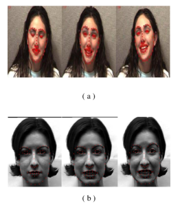
Figure 1: a) Some examples for RU-FACS database, b) Some examples for CK+ databases

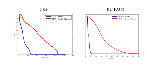
Figure 2: Convergence with respect to number of iterations for each datset

is more an expression dataset and is more challenging than the CK+ dataset, and it consists of facial behavior recorded during interviews. The interviews are about two minutes. Participants show moderate pose variation and speech-related mouth movements. Compared with the CK+ datasets, RU-FACS is more natural in timing, much longer, and the AUs are at lower intensity. For technical reasons, we selected from 29 of 34 participants with sequence length of about 7000 frames. Some examples from this database is shown in Figure 1.

VI Results

In this section we report the results based on two expression datasets. Figure 2 shows the number of iterations needs for convergence for each dataset. As can be seen in compare to ordinary GCRF our proposed model converges very fast even for a long time dataset (RU-FACS). Table I compares the area under ROC curve for the proposed databases. As can be seen the proposed model outperforms ordinary GCRF on two datasets.

VII Conclusion

In this paper the problem of temporal analysis is addressed. Many methods have been proposed in literature that have their own advantages and disadvantages. one of these methods which has been well studied in recognition and detection is GCRF. The problem with this method is the high computational cost for learning parameters. In this work we tackle this problem and we introduce a new model based on using ADMM. We evaluated our works on two publicly datasets and we show how our method converge fast in compare to ordinary GCRF. Also our proposed model outperforms GCRF.

Table I: Area under ROC curve for two expression databases

References

- [1] A. Asthana, S. Zafeiriou, S. Cheng, and M. Pantic. Robust discriminative response map fitting with constrained local models. In Computer Vision and Pattern Recognition (CVPR), 2013 IEEE Conference on, pages 3444–3451. IEEE, 2013.
- [2] M. S. Bartlett, G. C. Littlewort, M. G. Frank, C. Lainscsek, I. R. Fasel, and J. R. Movellan. Automatic recognition of facial actions in spontaneous expressions. Journal of Multimedia, 1(6):22–35, 2006.
- [3] S. Boyd, N. Parikh, E. Chu, B. Peleato, and J. Eckstein. Distributed optimization and statistical learning via the alternating direction method of multipliers. Foundations and Trends® in Machine Learning, 3(1):1–122, 2011.
- [4] S. Carlsson and J. Sullivan. Action recognition by shape matching to key frames. In Workshop on Models versus Exemplars in Computer Vision, volume 1, page 18, 2001.
- [5] H. Dibeklioğlu, A. A. Salah, and T. Gevers. Are you really smiling at me? spontaneous versus posed enjoyment smiles. In Computer Vision–ECCV 2012, pages 525–538. Springer, 2012.
- [6] J. Lafferty, A. McCallum, and F. C. Pereira. Conditional random fields: Probabilistic models for segmenting and labeling sequence data. 2001.
- [7] P. Lucey, J. F. Cohn, T. Kanade, J. Saragih, Z. Ambadar, and I. Matthews. The extended cohn-kanade dataset (ck+): A complete dataset for action unit and emotion-specified expression. In Computer Vision and Pattern Recognition Workshops (CVPRW), 2010 IEEE Computer Society Conference on, pages 94–101. IEEE, 2010.
- [8] L. Rabiner and B.-H. Juang. An introduction to hidden markov models. ASSP Magazine, IEEE, 3(1):4–16, 1986.
- [9] S. Roth and M. J. Black. Fields of experts: A framework for learning image priors. In Computer Vision and Pattern Recognition, 2005. CVPR 2005. IEEE Computer Society Conference on, volume 2, pages 860–867. IEEE, 2005.
- [10] K. Sikka, T. Wu, J. Susskind, and M. Bartlett. Exploring bag of words architectures in the facial expression domain. In Computer Vision–ECCV 2012. Workshops and Demonstrations, pages 250–259. Springer, 2012.
- [11] M. F. Tappen, C. Liu, E. H. Adelson, and W. T. Freeman. Learning gaussian conditional random fields for low-level vision. In Computer Vision and Pattern Recognition, 2007. CVPR’07. IEEE Conference on, pages 1–8. IEEE, 2007.
- [12] M. F. Valstar, I. Patras, and M. Pantic. Facial action unit detection using probabilistic actively learned support vector machines on tracked facial point data. In Computer Vision and Pattern Recognition-Workshops, 2005. CVPR Workshops. IEEE Computer Society Conference on, pages 76–76. IEEE, 2005.
- [13] M. Wytock and Z. Kolter. Sparse gaussian conditional random fields: Algorithms, theory, and application to energy forecasting. In Proceedings of the 30th International Conference on Machine Learning (ICML-13), pages 1265–1273, 2013.
- [14] N. Zhu, Z. Ma, and S. Wang. Dynamic characteristics and energy performance of buildings using phase change materials: A review. Energy Conversion and Management, 50(12):3169–3181, 2009.
- [15] S. C. Zhu, Y. Wu, and D. Mumford. Filters, random fields and maximum entropy (frame): Towards a unified theory for texture modeling. International Journal of Computer Vision, 27(2):107–126, 1998.