Depth, balancing, and limits of the Elo model

Abstract

Much work has been devoted to the computational complexity of games. However, they are not necessarily relevant for estimating the complexity in human terms. Therefore, human-centered measures have been proposed, e.g. the depth. This paper discusses the depth of various games, extends it to a continuous measure. We provide new depth results and present tool (given-first-move, pie rule, size extension) for increasing it. We also use these measures for analyzing games and opening moves in Y, NoGo, Killall Go, and the effect of pie rules.

I Introduction

Combinatorial or computational measures of complexity are widely used for games, specific parts of games, or families of games [kasai79, HearnDemaine2009, Viglietta2012, BonnetJamainSaffidine2013IJCAI]. Nevertheless, they are not always relevant for comparing the complexity of games from a human point of view:

• we cannot compare various board sizes of a same game with complexity classes P, NP, PSPACE, EXP, …because they are parametrized by the board size; and for some games (e.g. Chess) the principle of considering an arbitrary board size does not make any sense.

• state space complexity is not always clearly defined (for partially observable games), and does not indicate if a game is hard for computers or requires a long learning.

In Section II, we investigate another perspective that aims at better reflecting a human aspect on the depth of games. Section II-A defines the depth of games and the related Playing-level Complexity (PLC) is described in Section II-B. In Section LABEL:somegames we review the complexity of various games. In Section LABEL:boardsize we see the impact of board size on complexity. In Section LABEL:govskag, we compare the depth of Killall-Go to the depth of Go.

In Section LABEL:th, we analyze how various rules concerning the first move impact the depth and PLC. We focus on the pie rule (PR), which is widely used for making games more challenging, more balanced.

Then, we switch to experimental works in Section LABEL:prxp. We study in Section LABEL:sec:altering how the PR alters the PLC of existing games such as NoGo, Y, and Chinese Dark Chess (Fig. 1). Section LABEL:dkg then analyzes the depth and PLC of Killall-Go, in particular when using PR.

(a) NoGo

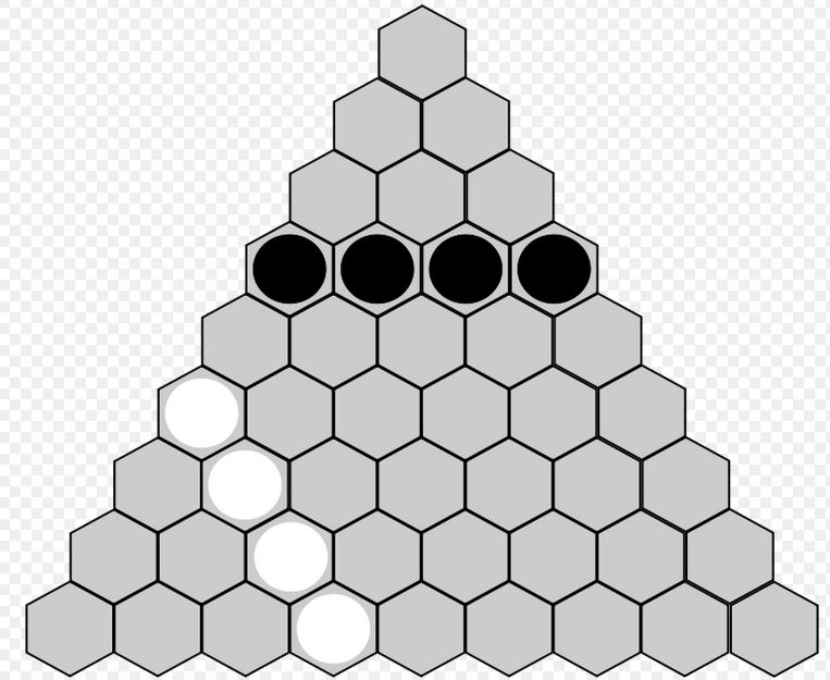
(b) Y

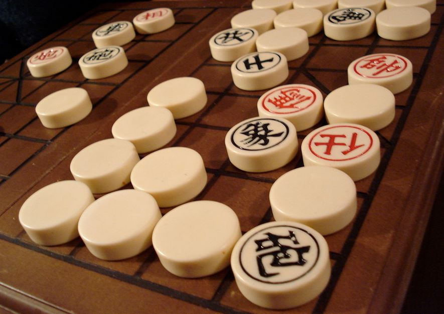
(c) Chinese Dark Chess

Figure 1: The NoGo, Y (2 variants) and Chinese Dark Chess games respectively. NoGo has a gameplay similar to Go, but capturing is forbidden which completely changes the strategy (this game is a win by BobNogo against NdhuNogo, July 2012 tournament). Y is a connection game: players play in turn and the first player who connects 3 sides wins (corners are connected to both sides). Chinese Dark Chess is related to Chinese Chess, but with hidden pieces; a special move consists in turning a face-down piece into face-up. Sources: Wikipedia and Kgs.

In all the paper, a rational choice means a choice which maximizes the success rate. This is the behavior of a player willing to win and having access to all possible information. In many cases below, we will assume that the opening moves and the pie rule choices (to swap or not to swap) are rational. In all the paper, $\log$ denotes logarithm with basis $10$.

II Human-centered complexity measures

In this section, we review some human-centered complexity measures for games: the depth and the playing level complexity.

II-A Definition of the depth of a game

Definition 1

Consider a game $G$, and a set $S$ of players. Then the depth $\Delta$ of $G$ is the maximal size of a set $p_{1},\dots,p_{\Delta}$ of players in $S$ such that for each $i$, $p_{i}$ wins with probability $\geq 60\%$ against $p_{i+1}$.

This measure was used in particular in [depth]. This definition is less than definitive: the depth of a game depends on whether we consider computer players, or just humans, and among them, any possible player, or only players playing in a “reasonable” manner. Also, many stupid games can be very deep for this measure: for example, who was born first, or who has the largest bank account number, or who has the first name in alphabetic order. The depth depends on the set of players. Let us consider an example showing that most games are extremely deep for this measure, if we consider the depth for all possible players. If, using the gameplay, players can exchange $b$ bits of information, then one can build $1,\dots,2^{b}$ players $p_{1},\dots,p_{d}$, with $p_{i}$ winning almost surely against $p_{i+1}$, as follows:

• First, $p_{i}$ starts by writing $i$ on $b$ bits of information (in Go, $p_{i}$ might encode this on the top of the board if he is black, and on the bottom of the board if he is white);

• Second, if the opponent has written $j<i$, then $p_{i}$ resigns.

This ensures an exponential depth of Go on an $n\times n$ board (and much better than this exponential lower bound is possible), with very weak players only. So, with no restrictions on the set of players, depth makes no sense.

An advantage of depth, on the other hand, is that it can compare completely unrelated games (Section LABEL:somegames) or different board sizes for a same game (Section LABEL:sec:impact-size).

II-B Playing-level complexity

We now define a new measure of game complexity, namely the playing level complexity (PLC).

Definition 2

The PLC of a game is the difference between the Elo rating of the strongest player and the Elo rating of a naive player for that game. More precisely, we will here use, as a PLC, the difference between the Elo rating of the best available player (in a given set) and the Elo rating of the worst available player (in the same set).

This implies that the PLC of a game depends on the set of considered players, as for the classical depth of games. An additional requirement is that the notion of best player and the notion of worst player make sense - which is the case when the Elo model applies, but not all games verify, even approximately, the Elo model (see a summary on the Elo model in Section LABEL:conc).

When the Elo model holds, the PLC is also equal to the sum of the pairwise differences in Elo rating: if players have ratings $r_{1}<r_{2}<\dots<r_{n}$, then the playing level complexity is $plc=r_{n}-r_{1}=\sum_{i=1}^{n-1}(r_{i+1}-r_{i})$. Applying the Elo classical formula, this means

$$plc=-\sum_{i=1}^{n-1}400\log(1/P_{i+1,i}-1),$$ (1)

where $P_{i+1,i}$ is the probability that player $i+1$ wins against player $i$. When the Elo model applies exactly, this is exactly the same as

$$plc=-400\log(1/P(strongest\ wins\ vs\ weakest)-1).$$ (2)

While both equations are equal in the Elo framework, they differ in our experiments and Eq. 1 is closer to depth results.

Unlike the computational complexity and just as the state-space complexity, the PLC allows to compare different board sizes for the same game. We can also use the PLC to compare variants that cannot be compared with the state-space complexity, such as different starting positions or various balancing rules, e.g. imposed first move or pie rules.

When the Elo model applies, the PLC is related to the depth. Let us see why. Let us assume that: (i) the Elo model applies to the game under consideration, (ii) there are infinitely many players, with players available for each level in the Elo range from a player $A$ (weakest) to a player $B$ (strongest). Then, the depth $\Delta$ of the game, for this set of players, is proportional to the PLC:

$$\Delta=1+\left\lfloor\frac{plc}{-400\log(\nicefrac{{1}}{{.6}}-1)}\right\rfloor=\left\lfloor\frac{Elo(B)-Elo(A)}{-400\log(\nicefrac{{1}}{{.6}}-1)}\right\rfloor.$$

.6 comes from the 60%. The ratio is $-400\log(\nicefrac{{1}}{{.6}}-1)\simeq.70.437$. Incidentally, we see that the PLC extends the depth in the sense that non-integer “depths” can now be considered.

TABLE I: Left: lower bounds on the PLC and depth for some widely played games. For Leagues of Legends the results are based on the Elo rating at the end of season 2 (data from the website competitive.na.leagueoflegends.com). Right: Analysis of the PR for NoGo and Y.

Game	PLC	D.
Go $19\times 19$		$\geq$ 40
Chess	$2300$	$\geq$ 16
Go $9\times 9$	$2200$	$\geq$ 14
Ch. Chess		$\geq$ 14
Shogi		$\geq$ 11
L.o. Legends	$1650$	$\geq 10$