Enhanced Low-Rank Matrix Approximation

Abstract

This letter proposes to estimate low-rank matrices by formulating a convex optimization problem with non-convex regularization. We employ parameterized non-convex penalty functions to estimate the non-zero singular values more accurately than the nuclear norm. A closed-form solution for the global optimum of the proposed objective function (sum of data fidelity and the non-convex regularizer) is also derived. The solution reduces to singular value thresholding method as a special case. The proposed method is demonstrated for image denoising.

I Introduction

Approximating a given matrix by a low-rank matrix is a fundamental problem in many signal processing applications [26, 37, 1, 22, 18, 40, 39]. The low-rank matrix approximation (LRMA) problem is a pivotal step in numerous machine learning [28, 16, 19, 17], statistical signal processing [5, 51, 46, 13, 50, 45], graph signal processing [8], and tensor recovery [25] problems. We consider the problem of estimating a low-rank matrix $X$ from its noisy observation $Y$,

$$Y=X+W,\quad X,Y,W\in\mathbb{R}^{m\times n}$$ (1)

where $W$ represents zero-mean additive white Gaussian noise (AWGN). We define the LRMA problem as

$$\arg\min_{X}\left\{\Psi(X)=\frac{1}{2}\|Y-X\|_{F}^{2}+\lambda\sum_{i=1}^{k}\phi(\sigma_{i}(X);a)\right\},$$ (2)

where $k=\min(m,n)$, $\sigma_{i}(X)$ is the i${}^{\text{th}}$ singular value of the matrix $X$, and $\phi$ is a sparsity-inducing regularizer, possibly non-convex. The standard nuclear norm minimization (NNM) problem [6] is a special case of the LRMA problem (2), with $\phi(x)=|x|$. Note that the NNM problem is convex and its global minimum can be directly obtained using the singular value decomposition (SVD) of the input matrix $Y$. In particular, if $Y=U\Sigma V^{T}$ is the SVD of $Y$, then the solution to the NNM problem is given by

$$\hat{X}=U\cdot\mbox{soft(}\Sigma;\lambda)\cdot V^{T}$$ (3)

where $\mbox{soft(}\cdot;\cdot)$ is the soft-threshold function [15] applied to the singular values of $Y$. The solution (3) to the NNM problem is known as ‘Singular Value Thresholding’ (SVT) method [6].

The SVT method tends to underestimate the non-zero singular values. Several recent studies have emphasized the benefit of non-convex penalty functions compared to the nuclear norm for the estimation of singular values [34, 33, 52, 7]. However, the use of non-convex penalty functions generally suffers from numerous issues (spurious local minima, initialization issues, etc.).

In this letter, we aim to estimate the non-zero singular values more accurately than the nuclear norm, while maintaining convexity of the objective function. To this end, we propose to use a particular class of parameterized non-convex penalty functions. We show how to set the non-convex penalty parameter to ensure the proposed objective function (2) is strictly convex. The idea of using non-convex penalty functions within a convex optimization framework was described by Blake and Zisserman [3] and Nikolova [42], and has been applied to various signal processing problems [48, 43, 44, 30, 23].

I-A Related Work

Several non-convex penalty functions have been utilized for the LRMA problem (2): the weighted nuclear norm [21], transformed Schatten-1 (TS1) [55] and the proximal p-norm [7]. The use of these non-convex penalty functions makes the overall LRMA problem non-convex. As such, iterative algorithms aiming to reach a stationary point (i.e., not necessarily global optimum) of the non-convex objective function have been developed [55, 21]. Also, a non-iterative locally optimal solution for the LRMA problem using the proximal p-norm is reported in [7]. Note that the proximal operators (see Sec. II-A) associated with the TS1 penalty and the proximal p-norm are not continuous for all values of the regularization parameter $\lambda$. In contrast, the proposed approach always leads to a convex problem formulation. A broader class of non-convex penalty functions was studied for the LRMA problem (2) in [52, 33, 32]. The iteratively reweighted nuclear norm minimization [34, 32] and generalized singular value thresholding [33] methods provide a locally optimal solution to the LRMA problem, provided that the penalty functions satisfy certain assumptions (see Assumption A1 of [34]).

II Preliminaries

We denote vectors and matrices by lower and upper case letter respectively. The Frobenius norm of a matrix $\mathnormal{Y}\in\mathbb{R}^{m\times n}$ is defined as

$$\|\mathnormal{Y}\|_{F}^{2} =\sum_{i=1}^{m}\sum_{j=1}^{n}|\mathnormal{Y}_{i,j}|^{2}$$ (4)

$$=\operatorname*{tr}(Y^{T}Y).$$ (5)

The nuclear norm of $Y$ is defined as

$$\|\mathnormal{Y}\|_{*}=\sum_{i=1}^{\min(m,n)}\sigma_{i}(\mathnormal{Y}),$$ (6)

where $\sigma_{i}(\mathnormal{Y})$ represents the $i^{\text{th}}$ singular value of $\mathnormal{Y}$.

II-A Penalty Functions, Proximity Operators

In order to estimate non-zero singular values more accurately, and induce sparsity more effectively, than the nuclear norm, we use non-convex penalty functions parameterized by the parameter $a\geqslant 0$ [47]. We make the following assumption on such penalty functions.

Assumption 1

The non-convex penalty function $\phi\colon\mathbb{R}\to\mathbb{R}$ satisfies the following properties

1. $\phi$ is continuous on $\mathbb{R}$, $\phi$ is continuously differentiable on $\mathbb{R}\setminus\{0\}$ and symmetric, i.e., $\phi(-x;a)=\phi(x;a)$

2. $\phi^{\prime}(x;a)\geqslant 0,\forall x>0$

3. $\phi^{\prime\prime}(x;a)\leqslant 0,\forall x>0$

4. $\phi^{\prime}(0^{+};a)=1$

5. $\inf\limits_{x\neq 0}\phi^{\prime\prime}(x;a)=\phi^{\prime\prime}(0^{+};a)=-a$

An example of a penalty function $\phi$ satisfying Assumption 1 is the partly quadratic penalty function [54, 2] defined as

$$\phi(x;a):=\begin{cases}|x|-\dfrac{a}{2}x^{2},&|x|\leqslant\frac{1}{a}\\ \dfrac{1}{2a},&|x|\geqslant\frac{1}{a}\end{cases}$$ (7)

Note that as $a\to 0$, the $\ell_{1}$ norm is recovered as a special case of this penalty. Several other examples of penalty functions satisfying Assumption 1 are listed in Table II of Ref. [9].

Definition 1

[10, 11]. Let $\phi\colon\mathbb{R}\to\mathbb{R}$ be a non-convex penalty function satisfying Assumption 1. The proximal operator of $\phi$, $\Theta:\mathbb{R}\to\mathbb{R}$, is defined as

$$\Theta(y;\lambda,a):=\arg\min_{x\in\mathbb{R}}\left\{\frac{1}{2}(y-x)^{2}+\lambda\phi(x;a)\right\}.$$ (8)

If $0\leqslant a<1/\lambda$, then $\Theta$ is a continuous non-linear threshold function with threshold value $\lambda$, i.e.,

$$\Theta(y;\lambda,a)=0,\quad\forall|y|<\lambda.$$ (9)

For example, the proximal operator of the partly quadratic penalty (7) is the firm threshold function [20] defined as

$$\Theta(y;\lambda,a):=\min\bigl{\{}|y|,\max\{(|y|-\lambda)/(1-a\lambda),0\}\bigr{\}}\text{sign}(y).$$

Note that for the matrix $\mathnormal{X}$, the notation $\Theta(X;\lambda,a)$ indicates that the proximal operator is applied element-wise to $\mathnormal{X}$.

III Low-rank matrix approximation

III-A Convexity condition

We note the following lemmas, which will be used to obtain a convexity condition for the objective function $\Psi$ in (2).

Lemma 1

[43]. Let $\phi\colon\mathbb{R}\to\mathbb{R}$ be a non-convex penalty function satisfying Assumption 1. The function $s\colon\mathbb{R}\to\mathbb{R}$ defined as

$$s(x;a):=\phi(x;a)-|x|,$$ (10)

is continuously differentiable, concave, and satisfies

$$-a\leqslant s^{\prime\prime}(x;a)\leqslant 0.$$ (11)

Lemma 2

Let $\phi\colon\mathbb{R}\to\mathbb{R}$ be a non-convex penalty function satisfying Assumption 1 and let $\lambda>0$. The function $f\colon\mathbb{R}\to\mathbb{R}$ defined as

$$f(x):=\dfrac{1}{2}x^{2}+\lambda\phi(x;a)$$ (12)

is strictly convex if

$$0\leqslant a<\dfrac{1}{\lambda}.$$ (13)

Proof:

Consider the function $g\colon\mathbb{R}\to\mathbb{R}$ defined as

$$g(x):=\dfrac{1}{2}x^{2}+\lambda s(x;a),$$ (14)

where the function $s$ is defined in (10). Note that

$$f(x) =\dfrac{1}{2}x^{2}+\lambda\phi(x;a)$$ (15)

$$=\dfrac{1}{2}x^{2}+\lambda\bigl{(}s(x;a)+|x|\bigr{)}$$ (16)

$$=g(x)+\lambda|x|.$$ (17)

In order to ensure the strict convexity of the function $f$, it is sufficient to ensure the strict convexity of the function $g$. To this end, it suffices to show that the second derivative of the function $g$ is positive, i.e. $g^{\prime\prime}(x)>0$ for all $x\in\mathbb{R}$. From (14), we note that $g^{\prime\prime}(x)>0$ if

$$1+\lambda s^{\prime\prime}(x;a)>0.$$ (18)

Using Lemma 1, $g^{\prime\prime}(x)>0$ for all $x\in\mathbb{R}$ if $0\leqslant a<1/\lambda$. Thus, the function $g$ (and hence the function $f$) is strictly convex if the parameter $a$ satisfies the inequality (13). ∎

The following theorem shows $a$ must satisfy (13) to ensure the strict convexity of the function $\Psi$ in (2).

Theorem 1

Let $\phi\colon\mathbb{R}\to\mathbb{R}$ be a non-convex penalty function satisfying Assumption 1. The objective function $\Psi\colon\mathbb{R}^{m\times n}\to\mathbb{R}$ in (2) is strictly convex if $0\leqslant a<1/\lambda.$

Proof:

We assume $m=n$. The derivation for $m\neq n$ is similar. Let $s\colon\mathbb{R}\to\mathbb{R}$ be defined as in Lemma 1. Consider the function $G\colon\mathbb{R}^{m\times n}\to\mathbb{R}$ defined as

$$G(X) =\dfrac{1}{2}\|Y-X\|_{F}^{2}+\lambda\sum_{i=1}^{m}s\bigl{(}\sigma_{i}(X);a\bigr{)}$$ (19)

$$=\dfrac{1}{2}\operatorname*{tr}\bigl{(}(Y-X)^{T}(Y-X)\bigr{)}+\lambda\sum_{i=1}^{m}s\bigl{(}\sigma_{i}(X);a\bigr{)}$$

$$=\dfrac{1}{2}\operatorname*{tr}(Y^{T}Y)-\operatorname*{tr}(XY^{T})+\dfrac{1}{2}\operatorname*{tr}(X^{T}X)$$

$$\qquad+\lambda\sum_{i=1}^{m}s\bigl{(}\sigma_{i}(X);a\bigr{)}.$$ (20)

Note that $\operatorname*{tr}(Y^{T}Y)$ does not depend on $X$ and $\operatorname*{tr}(XY^{T})$ is linear in $X$. Hence, the function $G$ is strictly convex if $G_{2}$ is strictly convex, where $G_{2}\colon\mathbb{R}^{m\times n}\to\mathbb{R}$ is defined as

$$G_{2}(X) =\dfrac{1}{2}\operatorname*{tr}(X^{T}X)+\lambda\sum_{i=1}^{m}s\bigl{(}\sigma_{i}(X);a\bigr{)}$$ (21)

$$=\dfrac{1}{2}\sum_{i=1}^{m}\sigma_{i}^{2}(X)+\lambda\sum_{i=1}^{m}s\bigl{(}\sigma_{i}(X);a\bigr{)}.$$ (22)

To ensure that the function $G_{2}$ is strictly convex, consider the function $h\colon\mathbb{R}^{m}\to\mathbb{R}$ defined as

$$h(x)=\sum_{i=1}^{m}g(x_{i}),$$ (23)

where $g$ is defined as in (14). Due to Lemma 2, the function $h$ is strictly convex and absolutely symmetric [31]. In view of (14), (22), and (23), the function $G_{2}$ can be written as

$$G_{2}(X) =\dfrac{1}{2}\sum_{i=1}^{m}\sigma_{i}^{2}(X)+\lambda\sum_{i=1}^{m}s\bigl{(}\sigma_{i}(X);a\bigr{)}$$ (24)

$$=\sum_{i=1}^{m}\biggl{(}\dfrac{1}{2}\sigma_{i}^{2}(X)+\lambda s\bigl{(}\sigma_{i}(X);a\bigr{)}\biggr{)}$$ (25)

$$=\sum_{i=1}^{m}g(\sigma_{i}(X))$$ (26)

$$=h(\sigma(X)),$$ (27)

where $\sigma(X)$ denotes the vector of singular values of the matrix $X$. From Corollary 2.6 of [31], since $h$ is absolutely symmetric, the unitarily invariant function $G_{2}(X)=h(\sigma(X))$ is strictly convex if and only if $h$ is strictly convex. It follows from Lemma 2 that $G_{2}$ (and hence $G$) is strictly convex if $a$ satisfies inequality (13).

Further, note that $\Psi$ in (2) can be written as

$$\Psi(X) :=\frac{1}{2}\|Y-X\|_{F}^{2}+\lambda\sum_{i=1}^{m}\phi(\sigma_{i}(X);a)$$ (28)

$$=\frac{1}{2}\|Y-X\|_{F}^{2}+\lambda\sum_{i=1}^{m}\Bigl{(}s(\sigma_{i}(X);a)+|\sigma_{i}(X)|\Bigr{)}$$

$$=\frac{1}{2}\|Y-X\|_{F}^{2}+\lambda\sum_{i=1}^{m}s(\sigma_{i}(X);a)+\lambda\sum_{i=1}^{m}|\sigma_{i}(X)|$$

$$=G(X)+\lambda\|X\|_{*}.$$ (29)

Hence, if $a$ satisfies (13), then the function $\Psi$ in (2) is strictly convex, being the sum of a convex function (the nuclear norm) and the strictly convex function $G$. ∎

III-B Global optimum

Theorem 1 ensures the proposed objective function $\Psi$ in the LRMA problem (2) is strictly convex if $0\leqslant a<1/\lambda$. The following theorem provides a closed-form solution to the proposed LRMA problem (2). The solution involves thresholding the singular values of the input matrix $Y$.

Theorem 2

Let $Y=U\Sigma V^{T}$ be the SVD of $Y$ and $\phi\colon\mathbb{R}\to\mathbb{R}$ be a non-convex penalty function satisfying Assumption 1. If $0\leqslant a<1/\lambda$, then the global minimizer of (2) is

$$\bar{X}=U\cdot\Theta(\Sigma;\lambda,a)\cdot V^{T},$$ (30)

where $\Theta$, defined in (8), is the threshold function associated with the non-convex penalty function $\phi$.

Proof:

We let $m=n$. The proof for $m\neq n$ is similar. Since $0\leqslant a<1/\lambda$, the function $\Psi$ in (2) is strictly convex; hence the minimizer of (2) is unique. Let

$$\Phi(X):=\sum_{i=1}^{m}\phi\bigl{(}\sigma_{i}(X);a\bigr{)}.$$ (31)

Note that for unitary matrices $U$ and $V$, $\Phi(X)=\Phi(UXV)$. Using the unitary invariant property of the Frobenius norm, and the SVD of $Y$, we write

$$\hat{X} =\arg\min_{X}\left\{\frac{1}{2}\|Y-X\|_{F}^{2}+\lambda\Phi(X)\right\}$$ (32)

$$=\arg\min_{X}\left\{\frac{1}{2}\|\Sigma-U^{T}XV\|_{F}^{2}+\lambda\Phi(U^{T}XV)\right\}$$ (33)

$$=U\cdot\arg\min_{X}\left\{\frac{1}{2}\|\Sigma-X\|_{F}^{2}+\lambda\Phi(X)\right\}\cdot V^{T}.$$ (34)

As a result of (34), we need to show that

$$\Theta(\Sigma;\lambda,a):=\arg\min_{X}\left\{\frac{1}{2}\|\Sigma-X\|_{F}^{2}+\lambda\Phi(X)\right\},$$ (35)

is the optimal solution. Note that with $Y=\Sigma$, (35) is strictly convex (as $0\leqslant a<1/\lambda$) from Theorem 1 and hence admits a unique global minimum. Let

$$X=U_{x}\Sigma_{x}V_{x}^{T},$$ (36)

be the SVD of $X$. We can write

$$\|\Sigma-X\|_{F}^{2} =\|X\|_{F}^{2}+\|\Sigma\|_{F}^{2}-2\operatorname*{tr}(X^{T}\Sigma)$$ (37)

$$\geqslant\|\Sigma_{x}\|_{F}^{2}+\|\Sigma\|_{F}^{2}-2\operatorname*{tr}(\Sigma_{x}\Sigma)$$ (38)

$$=\|\Sigma-\Sigma_{x}\|_{F}^{2}.$$ (39)

The inequality in (38) is due to von Neumann’s trace inequality. From (39), we note that

$$\frac{1}{2}\|\Sigma-X\|_{F}^{2}+\lambda\Phi(X)\geqslant\frac{1}{2}\|\Sigma-\Sigma_{x}\|_{F}^{2}+\lambda\Phi(\Sigma_{x}),$$ (40)

with equality if $X=\Sigma_{x}$. Note that $\Sigma_{x}$ is a diagonal matrix.

Consider the problem of finding such a diagonal matrix $\Sigma_{x}$ using the optimization problem

$$\arg\min_{\Sigma_{x}}\left\{\frac{1}{2}\|\Sigma-\Sigma_{x}\|_{F}^{2}+\lambda\Phi(\Sigma_{x})\right\}.$$ (41)

The optimization problem (41) is separable, as $\Sigma$ and $\Sigma_{x}$ are diagonal. Hence, the solution to (41) can be obtained by applying the threshold function $\Theta$ to the entries of $\Sigma$. Thus, the optimal solution to (41) is

$$\Theta(\Sigma;\lambda,a)=\arg\min_{\Sigma_{x}}\left\{\frac{1}{2}\|\Sigma-\Sigma_{x}\|_{F}^{2}+\lambda\Phi(\Sigma_{x})\right\}.$$ (42)

Using $X=\Theta(\Sigma;\lambda,a)$, we obtain the equality in (40). This completes the proof of (35). ∎

Note that due to the monotonocity of the threshold function, the solution (30) to the proposed LRMA problem (2) does not change the order of singular values.

IV Examples

IV-A Synthetic data

We apply the proposed enhanced low-rank matrix approximation (ELMA) method on synthetic data to assess its performance. For the following example, we generate 15 realizations of a random matrix $M\in\mathbb{R}^{m\times n}$ with rank $k$, such that

$$M:=AB,\quad A\in\mathbb{R}^{m\times k},B\in\mathbb{R}^{k\times n}.$$ (43)

The matrices $A$ and $B$ are random matrices with entries chosen from an i.i.d normal distribution. We let $M$ be a $200\times 200$ matrix with rank 100. We add white Gaussian noise ($1\leqslant\sigma\leqslant 10$) to the matrix $M$, thus creating the noisy observation matrix $Y$. We use the normalized root square error (RSE) defined as $\mbox{RSE}=\|X-M\|_{F}/\|M\|_{F}$, as a performance measure.

Figure 1: Average RSE as a function of the noise level ($\sigma$).

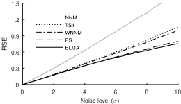
We compare the proposed ELMA method to the weighted nuclear norm minimization (WNNM) [21], standard nuclear norm minimization (NNM) [6], p-shrinkage (PS) [7] and the TS1 [55] LRMA methods. For the ELMA, NNM and PS methods, we set $\lambda=\beta\sigma$, where $\beta$ is manually set to optimize the RSE for each method. We use ELMA with the partly quadratic penalty (7) with $a=0.6/\lambda$ (i.e., we use the firm threshold function [20]). For the PS method, we use $p=-2$. For the WNNM method, we set the weights inversely proportional to the singular values of the input matrix, as suggested in [21]. Figure 1 shows the average RSE for the different methods. The proposed ELMA method yields the lowest RSE values for most values of $\sigma$.

IV-B Image Denoising

We consider denoising an image $X$ from its noisy observation $Y$, where the noise is AWGN with noise level $\sigma$. Recently, a growing number of image denoising methods are emerging based on the non-local self similarity (NSS) approach [4, 53, 36, 27]. State of the art image denoising algorithms such as BM3D [12], LSSC[35], NCSR[14], and PLR [24] are NSS based methods.

For a local patch in a noisy image $Y$, denote the matrix formed by stacking non-local similar patches as $Y_{j}$. The non-local similar patches can be found using block matching methods [12]. As such, we write $Y_{j}=X_{j}+W_{j}$, where $X_{j}$ is the patch matrix of the clean image and $W_{j}$ is AWGN. In order to estimate $X_{j}$ from $Y_{j}$, we propose the following objective function, similar to Eq. (9) of [21],

$$\hat{X}_{j}:=\arg\min_{X}\left\{\frac{1}{2}\|Y_{j}-X\|_{F}^{2}+\lambda\sum_{i=1}^{m}\phi(\sigma_{i}(X);a)\right\}.$$ (44)

The objective function in (44) is strictly convex if $a<1/\lambda$, from Theorem 1. Further, with $Y_{j}=U_{j}\Sigma_{j}V_{j}^{T}$ as the SVD of $Y_{j}$, the solution to (44) is given by $\hat{X}_{j}=U_{j}\Theta(\Sigma_{j};\lambda,a)V_{j}^{T}$, as per Theorem 2.

We perform image denoising using ELMA to estimate each patch matrix $X_{j}$. We compare the denoised images obtained using ELMA with the denoised images obtained using BM3D, PS, NNM and the WNNM methods. We use three test images of size $512\times 512$ and add AWGN with $\sigma=100$. We set the regularization parameter $\lambda$ in (44) as in the previous example.

Figure 2: Denoised ‘Barbara’ image using several LRMA methods within the NSS framework. (a) BM3D (b) WNNM (c) p-shrinkage (d) ELMA (proposed).

TABLE I: Average PSNR (dB) obtained by several image denoising methods.

Image	Method
	BM3D	PS	NNM	WNNM	ELMA
Boat	23.97	23.82	22.88	24.10	24.03
Barbara	23.62	23.55	22.98	24.37	24.46
Couple	23.51	23.35	22.07	23.57	23.53

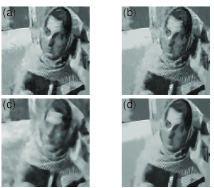
Figure 2 shows the denoised ‘Barbara’ image using several LRMA methods. The average PSNR values for the three test images are listed in Table I. The proposed ELMA method achieves higher PSNR than the BM3D, PS, and NNM methods. On average, the PSNR values obtained by the ELMA method are comparable to those obtained by the WNNM method. However, in terms of the image quality, the proposed ELMA method contains fewer artifacts.

V Conclusion

This letter proposes a method to estimate low-rank matrices corrupted with AWGN. The proposed method, which outperforms nuclear norm minimization, is based on an objective function comprising a data-fidelity term and a non-convex regularizer. The proposed objective function is convex even though the regularizer is not. The non-iterative solution to the proposed objective function is obtained by thresholding the singular values of the input matrix. We demonstrate the effectiveness of the proposed method for image denoising by using it within a non-local self-similarity based image denoising algorithm. The proposed method has the same computational complexity as the SVT method. As such, scalable methods [49] to accelerate the computation may also be applicable to the proposed method.

Supplemental Figures

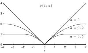
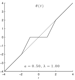
Figure 3 illustrates the particular penalty function $\phi(t;a)$ defined in (7) for several values of the parameter $a$. Figure 4 illustrates the threshold function (i.e., proximity operator) associated with this penalty. This is known as the firm threshold function.

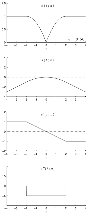
Figure 5 illustrates the penalty function and the corresponding function $s(t;a)$ defined in (10). The figure also shows the first and second-order derivatives of the function $s(t;a)$.

Figure 3: Penalty function $\phi(t;a)$ for several values of $a$.

Figure 4: Firm threshold function.

Figure 5: Penalty $\phi(t;a)$ and function $s(t;a)=\phi(t;a)-|t|$ for $a=0.5$.

References

- [1] D. Achlioptas and F. McSherry, “Fast computation of low rank matrix approximations,” in Proc. ACM Symp. Theory Comput., pp. 611–618, 2001.
- [2] I. Bayram, “On the convergence of the iterative shrinkage/thresholding algorithm with a weakly convex penalty,” IEEE Trans. Signal Process., early access, 2015.
- [3] A. Blake and A. Zisserman, “Visual reconstruciton,” MIT Press, 1987.
- [4] A. Buades, B. Coll, and J. M. Morel, “A non-local algorithm for image denoising,” in Proc. IEEE Comput. Vis. Pattern Recognit., vol. 2, pp. 60–65, 2015.
- [5] J. Cadzow, “Signal enhancement - A composite property mapping algorithm,” IEEE Trans. Acoust., vol. 36, no. 1, pp. 49–62, 1988.
- [6] J.-F. Cai, E. J. Candes, and Z. Shen, “A singular value thresholding algorithm for matrix completion,” SIAM J. Optim., vol. 20, no. 4, pp. 1–26, 2008.
- [7] R. Chartrand, “Nonconvex splitting for regularized low-rank + sparse decomposition,” IEEE Trans. Signal Process., vol. 60, no. 11, pp. 5810–5819, 2012.
- [8] S. Chatterjee, “Matrix estimation by universal singular value thresholding,” Ann. Stat., vol. 43, no. 1, pp. 177–214, 2015.
- [9] P.-Y. Chen and I. W. Selesnick, “Group-sparse signal denoising: Non-convex regularization, convex optimization,” IEEE Trans. Signal Process. vol. 62, no. 13, pp. 3464-3478, Jul. 2014.
- [10] P. L. Combettes and J.-C. Pesquet, “Proximal thresholding algorithm for minimization over orthonormal bases,” SIAM J. Optim., vol. 18, no. 4, pp. 1351–1376, 2007.
- [11] P. L. Combettes and J.-C. Pesquet. “Proximal splitting methods in signal processing” in H. H. Bauschke et al., editors, Fixed-Point Algorithms for Inverse Problems in Science and Engineering, Springer-Verlag, pp. 185-–212, 2011.
- [12] K. Dabov, A. Foi, V. Katkovnik, and K. Egiazarian, “Image denoising by sparse 3-D transform-domain collaborative filtering,” IEEE Trans. Image Process. , vol. 16, no. 8, pp. 2080–2095, 2007.
- [13] S. Dasgupta, “Learning mixtures of Gaussians,” IEEE Symp. Found. Comput. Sci., pp. 634-644, 1999.
- [14] W. Dong, L. Zhang, and G. Shi, “Centralized sparse representation for image restoration,” in Proc. IEEE Int. Conf. Comput. Vis., pp. 1259–1266, 2011.
- [15] D. L. Donoho, “De-noising by soft-thresholding,” IEEE Trans. Inf. Theory, vol. 41, no. 3, pp. 613–627, 1995.
- [16] P. Drineas, R. Kannan, and M. W. Mahoney, “Fast Monte Carlo algorithms for matrices II: Computing a low-rank approximation to a matrix,” SIAM J. Comput. vol. 36, no. 1 pp. 158–183, 2006.
- [17] R. Foygel and N. Srebro, “Concentration-based guarantees for low-rank matrix reconstruction,” Proc. Conf. Learn. Theory, vol. 19, no. 1, pp. 315–339, 2011.
- [18] M. Fazel, T. K. Pong, D. Sun, and P. Tseng, “Hankel matrix rank minimization with applications to system identification and realization,” SIAM J. Matrix Anal. Appl., vol. 34, no. 3, pp. 946–977, Jul. 2013.
- [19] R. Foygel, N. Srebro, and R. Salakhutdinov, “Matrix reconstruction with the local max norm,” Adv. Neural Inf. Process. Syst., pp. 935–943, 2012.
- [20] H. Y. Gao and A. G. Bruce. “Waveshrink with firm shrinkage,” Stat. Sinica, vol. 7, no. 4, pp. 855–874, 1997.
- [21] S. Gu, L. Zhang, W. Zuo, and X. Feng, “Weighted nuclear norm minimization with application to image denoising,” in IEEE Conf. Comput. Vis. Pattern Recognit., pp. 2862–2869, 2014.
- [22] A. Hansson, Z. Liu, and L. Vandenberghe, “Subspace system identification via weighted nuclear norm optimization,” Proc. IEEE Conf. Decis. Control, pp. 3439–3444, 2012.
- [23] W. He, Y. Ding, Y. Zi, and I. W. Selesnick, “Sparsity-based algorithm for detecting faults in rotating machines,” Mech. Syst. Signal Proc., vol. 72, pp. 46–64, 2016.
- [24] H. Hu, J. Froment, and Q. Liu, “Patch-based low-rank minimization for image denoising,” http://arxiv.org/abs/1506.08353, pp. 1–4, 2015.
- [25] B. Huang, C. Mu, D. Goldfarb, and J. Wright, “Provable models for robust low-rank tensor completion,” Pacific J. Optim., vol. 11, no. 2, pp. 339–364, 2015.
- [26] I.-Y. Jeong and K. Lee, “Vocal separation using extended robust principal component analysis with Schatten P/LP-norm and scale compression,” in Proc. Mach. Learn. Signal Process., pp. 1–7, 2014.
- [27] H. Ji, C. Liu, Z. Shen, and Y. Xu, “Robust video denoising using low rank matrix completion,” Proc. IEEE Comput. Vis. Pattern Recognit., pp. 1791–1798, 2010.
- [28] R. Kannan and S. Vempala, “Spectral Algorithms,” Found. Trends Theor. Comput. Sci., vol. 4, no. 3–4, pp. 157–288, 2008.
- [29] D. Krishnan and R. Fergus, “Fast image deconvolution using hyper-Laplacian priors,” Proc. Nerual Inf. Process. Syst., pp. 1033–1041, 2009.
- [30] A. Lanza, S. Morigi, and F. Sgallari, “Convex image denoising via non-convex regularization,” in J.-F. Aujol, M. Nikolova, and N. Papadakis, editors, Scale Space and Variational Methods in Computer Vision, ser. Lecture Notes in Computer Science, Springer, vol. 9087, pp. 666–677, 2015.
- [31] A. S. Lewis, “The convex analysis of unitarily invariant matrix functions.” J. Convex Anal., vol. 2, no. 1–2, pp. 173–183, 1995.
- [32] C. Lu, J. Tang, S. Yan, and Z. Lin, “Nonconvex nonsmooth low rank minimization via iteratively reweighted nuclear norm,” IEEE Trans. Image Process., vol. 25, no. 2, pp. 829–839, Feb. 2016.
- [33] C. Lu, J. Tang, S. Yan, and Z. Lin, “Generalized nonconvex nonsmooth low-rank minimization,” in IEEE Conf. Comput. Vis. Pattern Recognit., pp. 4130–4137, Jun. 2014.
- [34] C. Lu, C. Zhu, C. Xu, S. Yan, and Z. Lin, “Generalized singular value thresholding,” AAAI Conf. Artif. Intell., Jan. 2015.
- [35] J. Mairal, F. Bach, J. Ponce, G. Sapiro, and A. Zisserman, “Non-local sparse models for image restoration,” in Proc. IEEE Int. Conf. Comput. Vis., pp. 2272–2279, 2009.
- [36] J. V. Manjón, J. Carbonell-Caballero, J. J. Lull, G. García-Martí, L. Martí-Bonmatí et al., “MRI denoising using non-local means,” Med. Image Anal., vol. 12, no. 4, pp. 514–523, 2008.
- [37] I. Markovsky, “Structured low-rank approximation and its applications,” Automatica, vol. 44, no. 4, pp. 891–909, 2008.
- [38] K. Mohan and M. Fazel, “Iterative reweighted algorithms for matrix rank minimization,” J Mach. Learn. Res., vol. 13, no. 1, pp. 3441–3473, Jan. 2012.
- [39] R. R. Nadakuditi, “Optshrink: An algorithm for improved low-rank signal matrix denoising by optimal, data-driven singular value shrinkage,” IEEE Trans. Inf. Theory, vol. 60, no. 5, pp. 3002–3018, May 2014.
- [40] H. M. Nguyen, X. Peng, M. N. Do, and Z.-P. Liang, “ Denoising MR spectroscopic imaging data with low-rank approximations,” IEEE Trans. Biomed. Eng., vol. 60, no. 1, pp. 78–89, 2013.
- [41] F. Nie, H. Wang, X. Cai, H. Huang, and C. Ding, “Robust matrix completion via joint Schatten p-Norm and lp-norm minimization,” in IEEE Int. Conf. Data Min., pp. 566–574, 2012.
- [42] M. Nikolova, “Estimation of binary images by minimizing convex criteria,” Proc. IEEE Int. Conf. Image Process. (ICIP), vol. 2, 1998.
- [43] A. Parekh and I. W. Selesnick, “Convex denoising using non-convex tight frame regularization,” IEEE Signal Process. Lett., vol. 22, no. 10, pp. 1786–1790, 2015.
- [44] A. Parekh and I. W. Selesnick, “Convex fused lasso denoising with non-convex regularization and its use for pulse detection,” IEEE Symp. Sig. Proc. Med. Biol., pp. 1–6, Dec. 2015.
- [45] E. Richard, E. C. Paris, N. Vayatis, and P.-A. Savalle, “Estimation of simultaneously sparse and low rank matrices,” Proc. Int. Conf. Mach. Learn., pp. 1351–1358, 2012.
- [46] A. Sanjeev and R. Kannan, “Learning mixtures of arbitrary Gaussians,” in Proc. ACM Symp. Theory Comput., pp. 247–257, 2001.
- [47] I. W. Selesnick and I. Bayram, “Sparse signal estimation by maximally sparse convex optimization,” IEEE Trans. Signal Process., vol. 62, no. 5, pp. 1078–1092, 2014.
- [48] I. W. Selesnick, A. Parekh, and I. Bayram, “Convex 1-D total variation denoising with non-convex regularization,” IEEE Signal Process. Lett., vol. 22, no. 2, pp. 141–144, 2015.
- [49] F. Shang, Y. Liu, and J. Cheng, “Scalable algorithms for tractable Schatten quasi-norm minimization,” AAAI Conf. Artif. Intell., Jan. 2016.
- [50] M. E. Tipping and C. M. Bishop, “Mixtures of probabilistic principal component analyzers.” Neural Comput., vol. 11, no. 2, pp. 443–482, 1999.
- [51] S. Vempala and G. Wang, “A spectral algorithm for learning mixtures of distributions,” in Proc. IEEE Symp. Found. Comput. Sci., 2002.
- [52] S. Wang, D. Liu, and Z. Zhang, “Nonconvex relaxation approaches to robust matrix recovery,” Int. Jt. Conf. Artif. Intell., pp. 1764–1770, 2013.
- [53] Z. Yang and M. Jacob, “Non-local regularization of inverse problems: A unified variational framework,” IEEE Trans. Image Process., vol. 22, no. 8, pp. 3192–3203, 2013.
- [54] C.-H. Zhang, “Nearly unbiased variable selection under minimax concave penalty,” Ann. Stat., vol. 38, no. 2, pp. 894–942, 2010.
- [55] S. Zhang, P. Yin, and J. Xin, “Transformed Schatten-1 iterative thresholding algorithms for matrix rank minimization and applications,” http://arxiv.org/abs/1506.04444, pp. 1–22, 2015.