Radon–Nikodym approximation in application to image reconstruction.

Abstract

$Id: RNimages.tex,v 1.105 2015/12/15 12:49:00 mal Exp $

For an image pixel information can be converted to the moments of some basis $Q_{k}$, e.g. Fourier–Mellin, Zernike, monomials, etc. Given sufficient number of moments pixel information can be completely recovered, for insufficient number of moments only partial information can be recovered and the image reconstruction is, at best, of interpolatory type. Standard approach is to present interpolated value as a linear combination of basis functions, what is equivalent to least squares expansion. However, recent progress in numerical stability of moments estimation allows image information to be recovered from moments in a completely different manner, applying Radon–Nikodym type of expansion, what gives the result as a ratio of two quadratic forms of basis functions. In contrast with least squares the Radon–Nikodym approach has oscillation near the boundaries very much suppressed and does not diverge outside of basis support. While least squares theory operate with vectors $<fQ_{k}>$, Radon–Nikodym theory operates with matrices $<fQ_{j}Q_{k}>$, what make the approach much more suitable to image transforms and statistical property estimation.

I Introduction

Image information representation is a fundamental question of image processing and analysis. Most common basis is pixel basis. However given basis functions $Q_{k}$ (e.g. Fourier, Zernike, orthogonal polynomialsTotik (11 Nov. 2005), etc.) image pixel information can be transformed to the moments of the basisMukundan and Ramakrishnan (1998); Pinoli (2014); Honarvar et al. (2014). Given sufficient number of moments a complete one-to-one mapping between pixel and moments information can be established. However, given limited number of moments a question arise: how image information can be recovered from moments available. Most common approach – representation of the result in a form of linear combination of basis functions, what is equivalent to least squares approximation. However, there is exist a different approach based on Radon–Nikodym derivativesKolmogorov and Fomin (8 May 2012) and its special case Nevai OperatorNevai (1979, 1986), where the result is represented as a ratio of two quadratic forms of basis functions. In contrast with least squares, which operate on vector moments $<fQ_{k}>$ of observable value $f$, the Radon–Nikodym approach operate with matrices $<fQ_{k}Q_{j}>$. Given recent progress in numerical stability of high order moments calculationMalyshkin and Bakhramov (2015) the matrices $<fQ_{k}Q_{j}>$ can now be calculated without any difficulty to a very high order and Radon–Nikodym become practically applicable to image processing. This matrix approach, has a number of unique features, such as suppression of typical for least squares oscillations near the boundary and improved numerical stability. In addition to that the transition from vector to matrix allows many image transforms to be easily expressed in terms of matrix $<fQ_{k}Q_{j}>$ transform and the approach allows to leverage matrix algebra in application to image processing.

II Basis expansion

Consider some feature $f$ (e.g. grayscale intensity), a basis $Q_{k}(x)$ (in 2D the basis would be $Q_{k_{x}}(x)Q_{k_{y}}(y)$) and the measure $\mu$ (in this paper the measure would be just the sum over the pixels). The moments are defined as:

$$<fQ_{k}> = \int\limits_{\mathrm{supp}(\mu)}fQ_{k}d\mu$$ (1)

The Gramm matrix is defined by the basis and the measure:

$$G_{ij}=<Q_{i}Q_{j}>$$ (2)

Then minimization of mean square difference between $f$ and its approximation $A_{LS}(x)$ obtain standard least squares result:

$$A_{LS}(x)=\sum_{i,j}Q_{i}(x)\left(G^{-1}\right)_{ij}<fQ_{j}>$$ (3)

Radon–Nikodym approximation $A_{RN}(x)$ can be obtained considering localized at $x_{0}$ states $\psi_{x_{0}}(x)$

$$\psi_{x_{0}}(x) = \frac{\sum_{i,j}Q_{i}(x)G^{-1}_{ij}Q_{j}(x_{0})}{\sqrt{\sum_{i,j}Q_{i}(x_{0})G^{-1}_{ij}Q_{j}(x_{0})}}$$ (4)

and a form of Radon–Nikodym approximation, Nevai OperatorNevai (1979, 1986), then becomes:

$$A_{RN}(x)=\frac{\sum_{i,j,k,m}Q_{i}(x)G^{-1}_{ij}<fQ_{j}Q_{k}>G^{-1}_{km}Q_{m}(x)}{\sum_{i,j}Q_{i}(x)G^{-1}_{ij}Q_{j}(x)}$$ (5)

The main idea is to consider localized at $x_{0}$ states $\psi_{x_{0}}(x)$, which is related to delta-function expanded in $Q_{k}(x)$ basis with measure (1), and perform $f$ reconstruction as $f(x_{0})\approx\int dxf(x)\psi^{2}_{x_{0}}(x)/\int dx\psi^{2}_{x_{0}}(x)$. Important, that integration weight $\psi^{2}_{x_{0}}(x)$ is always positive what supress oscillations typical for least squares, where the weight change sign. The $\psi_{x_{0}}(x)$ from (4) give exactly Nevai operator (5). For details and other $\psi_{x_{0}}(x)$ forms applicable for Radon–Nikodym estimation see Ref. Malyshkin and Bakhramov (2015). The (5), while is very different from least squares in concept, uses, nevertheless, almost the same input: Gramm matrix inverse $G^{-1}$ and $<Q_{i}Q_{k}f>$ matrix obtained from $<Q_{j}f>$ moments. The (5) is a ratio of two polynomial functions. It was shown in Ref. Malyshkin (2009) that in multi–dimensional signal processing stable estimators can be only of two quadratic forms ratio and the (5) is exactly of this form.

Let us apply least squares and Radon–Nikodym expressions to some real life cases.

II.1 1D Example: Runge Function.

Before we start considering 2D images, let us start with simple 1D example, take Runge function

$$f(x)=\frac{1}{1+25x^{2}}$$ (6)

Using the measure

$$<fQ_{k}> = \int_{-1}^{1}f(x)Q_{k}(x)dx$$ (7)

and the basis, for numerical stability of calculations, is chosen as Legendre polynomials $Q_{k}(x)=P_{k}(x)$ (given the measure all polynomial bases provide identical results, but numerical stability of calculations is different).

The $A_{RN}(x)$ calculation algorithm is this: given $N$ elements in basis using (7) definition calculate vector moments $<fQ_{m}>$ and $<Q_{m}>$ for $m=[0\dots 2N-1]$. Then, applying polynomials multiplication operation, for $j,k=[0\dots N-1]$ obtain matrix moments $<fQ_{j}Q_{k}>$ and $G=<Q_{j}Q_{k}>$ to be used in Eq. (3) and (5).

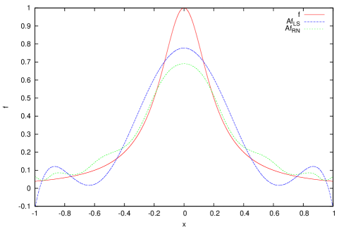
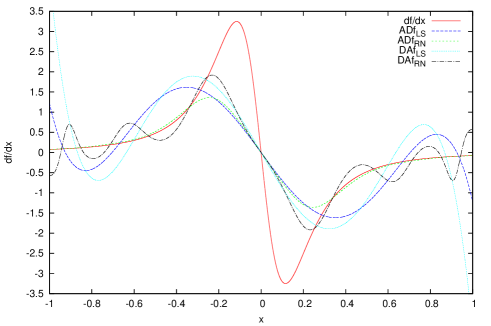
Figure 1: Top chart: Runge function $f$, least squares approximation $Af_{LS}$ and Radon–Nikodym approximation $Af_{RN}$. Bottom chart: Runge function derivative $\frac{df}{dx}$, least squares approximation $ADf_{LS}$ and Radon–Nikodym approximation $ADf_{RN}$ of the derivative $\frac{df}{dx}$. Differentiated interpolations of $f$ for least squares($DAf_{LS}$) and Radon–Nikodym ($DAf_{RN}$), that should not be used in applications are also presented as an example.

In top chart of Fig. 1 least squares and Radon–Nikodym interpolations are presented for $N=7$ and the measure (7). One can see that near edges oscillations are much less severe, when Radon–Nikodym approximation as polynomials ratio is used for the interpolation of $f$. The major behavior differences for least square and Radon–Nikodym approximations are: Least squares have diverging oscillations near measure support boundaries and tend to infinity with the distance to measure support increase. Radon–Nikodym have converging oscillations near measure support boundaries and tend to a constant with the distance to measure support increase.

Another, worth to mention point, is related to derivatives calculation. For this the moments $\left<Q_{k}\frac{df}{dx}\right>$ should be calculated first, and only then applying Radon–Nikodym approximation like (5) using derivative moments. If one, instead of using the $\left<Q_{k}\frac{df}{dx}\right>$ moments, would differentiate $f$ approximation expression (5) directly – the result will be incorrect. To illustrate the point in bottom chart of Fig. 1 least squares and Radon–Nikodym interpolations of Runge function derivative are presented for $N=7$ and measure (7). The differentiated approximations of Runge function are also presented.

The code calculating this 1D example is availableMalyshkin (2014), see the ExampleRungeFunction.scala file.

II.2 2D example: Lena image.

Let us consider 2D case of image grayscale intensity interpolation. Because the example is illustrative, let us take a sum over image pixels as the measure. As a basis, in principle, monomials $x^{k_{x}}y^{k_{y}}$ can be used, but for numerical stability reasons the basis should be chosen as orthogonal functions with respect to some measure. For an image of $d_{x}$ on $d_{y}$ pixels the moments of pixel–dependent grayscale intensity $f(t_{x},t_{y})$ (here $t_{x}=[0\dots d_{x}-1]$ and $t_{y}=[0\dots d_{y}-1]$ index pixel number) are:

$$<fQ_{k_{x},k_{y}}>=$$ (8)

$$\sum_{t_{x}=0}^{d_{x}-1}\sum_{t_{y}=0}^{d_{y}-1}f(t_{x},t_{y})Q_{k_{x}}(t_{x}/(d_{x}-1))Q_{k_{y}}(t_{y}/(d_{y}-1))$$

In the Eq. (8) the basis can be chosen as Legendre or Chebyshev polynomials shifted to $[0\dots 1]$ interval: $Q_{k}(x)=P_{k}(2x-1)$ and the argument of $Q$ is pixel coordinate converted to this interval: $x=t_{x}/(d_{x}-1)$ and $y=t_{y}/(d_{y}-1)$. When $d_{x}\to\infty$ $d_{y}\to\infty$ the Gramm matrix $<Q_{i_{x},i_{y}}Q_{j_{x},j_{y}}>$ is diagonal because of Legendre polynomials orthogonality and trivially invertable, but we used sample–calculated matrix, because the $d_{x}$ and $d_{y}$ can be rather small or when the basis is chosen as Chebyshev polynomials $Q_{k}(x)=T_{k}(2x-1)$. Note, that for a given measure all polynomial bases (e.g. Legendre, Chebyshev, monomials) give identical results, but numerical stability of calculations is drastically different, because Gramm matrix condition number depend strongly on basis choiceBeckermann (1996). For successful application in image reconstrcution Chebyshev moments see Ref. Mukundan et al. (2001) and for Legendre moments see Ref. Chiang and Liao (2014).

The numerical library we developed, seeMalyshkin and Bakhramov (2015) Appendix A, is able to manipulate polynomials in Chebyshev, Legendre, Laguerre and Hermite bases directly, what allows a stable basis to be used and calculate the moments to a very high order. Numerical calculations with polynomials in general basis were introduced in Maroulas and Barnett (1979) and similar technique was used in Laurie and Rolfes (1979) for Gauss quadratures calculation in Chebyshev basis. In this paper we used general polynomial basis approach (to achieve numerical stability) and applied it to Radon–Nikodym approximation calculation.

The $A_{RN}$ calculation algorithm is this: given image size $d_{x}$ and $d_{y}$ and basis dimension $N_{x}$ and $N_{y}$ using (8) definition calculate vector moments $<fQ_{m_{x},m_{y}}>$ and $<Q_{m_{x},m_{y}}>$ for $m_{x}=[0\dots 2N_{x}-1]$ and $m_{y}=[0\dots 2N_{y}-1]$. Then, applying polynomials multiplication operation, for $j_{x},k_{x}=[0\dots N_{x}-1]$ and $j_{y},k_{y}=[0\dots N_{y}-1]$ obtain matrix moments $<fQ_{j_{x},j_{y}}Q_{k_{x},k_{y}}>$ and $G=<Q_{j_{x},j_{y}}Q_{k_{x},k_{y}}>$ to be used in Eq. (3) and (5).

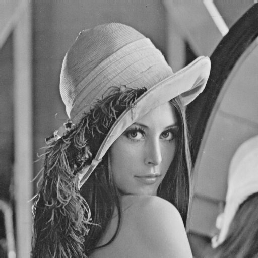
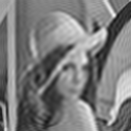
Figure 2: Original Lena image(top left), and for $N_{x}=N_{y}=50$ least squares(top right) and Radon-Nikodym (bottom). PNG originals are availabe from Malyshkin (2015).

Figure 3: Interplation of Lena image for $N_{x}=N_{y}=100$. Least squares(left) and Radon-Nikodym (right). PNG originals are availabe from Malyshkin (2015).

In Fig. 2 we present original 512x512 ($d_{x}=d_{y}=512$) grayscale Lena image, then for $N_{x}=N_{y}=50$ apply least squares (3) and Radon–Nikodym (5) transforms. Same calculations, but for $N_{x}=N_{y}=100$ are presented in Fig. 3. (The calculations for $N_{x}=N_{y}=100$ are rather slow, because we did not use any optimization, but the point of the paper is to demonstrate practical applicability of Radon–Nikodym type of interpolation and stability of high order moments calculation when a stable basis is chosen.)

The least squares interpolation, same as in 1D case, present typical for least squares intensity oscillations near image edges, while Radon–Nikodym has these oscillations very much supressed. Another important feature of Radon–Nikodym is that it preserves the sign of interpolated function, i.e. the grayscale intencity $f$ never become negative, what may happen easily for least squares. The code calculating this example is availableMalyshkin (2014), see the ExampleImageInterpolation.scala file. The calculations have been performed in both: Legendre and Chebyshev bases. For $N_{x}=N_{y}=50$ the results are identical, when interpolated grayscale is converted back to 1-byte values. For $N_{x}=N_{y}=100$ the results in two bases are almost identical (indistinguishable visually), but testing show that in Legendre basis numerical instabilities just started to show up in multiplication operation, because of factorial–like coefficients in $P_{n}(x)P_{m}(x)$ expansion. One can expect more instability in Legendre basis at $N_{x}=N_{y}>100$ (note, that for given $N$ we calculate $0..2N-1$ moments). In this sense Chebyshev multiplication $T_{n}(x)T_{m}(x)=\frac{1}{2}T_{n+m}(x)+\frac{1}{2}T_{|n-m|}(x)$ is special because the coeficients of product expansion do not grow or vanish for large $n;m$, so Chebyshev products can be stably calculated to a very high order and in the same time for discrete measures the Gramm matrix (2) posess a good condition numberBeckermann (1996) in this basis.

III Discussion and Natural Basis

In this paper we present a novel approach to image restoration from moments: the result is of Radon–Nikodym type where the result is a ratio of two quadracic forms of basis functions, and, in case of polynomial bases, is just two polynomials ratio. This approach, is based on matrices, not on vectors, what make calculations significantly more stable. In a way how Radon–Nikodym approach improved interpolation of a function, the transition from a vector $<Q_{k}f>$ to matrix $<Q_{j}Q_{k}f>$ can similary improve calculations of image properties, expressible through averages. Define an average $\overline{f}$ as:

$$\overline{f} = \frac{\mathrm{Spur}\left(\sum_{k}G_{jk}^{-1}<Q_{k}fQ_{l}>\right)}{\dim G}$$ (9)

$$= \frac{\sum_{j,k}G_{jk}^{-1}<Q_{k}fQ_{j}>}{\dim G}$$

where $\mathrm{Spur}$ is matrix trace (sum of diagonal elements) operator. The (9) definition can be also applied to estimation of an average of products, i.e.

$$\overline{fg}=\frac{\sum_{j,k,m,i}G_{jk}^{-1}<Q_{k}fQ_{m}>G_{mi}^{-1}<Q_{i}gQ_{j}>}{\dim G}$$ (10)

What allows image features cross–correlation to be expressed as matrix Spur. An important feature of the approach is that many image transforms can be easily expressed as a transform of matrix $<Q_{k}fQ_{m}>$ , what makes proposed matrix approach extremely practical, when a stable basis is chosen. Numerical library providing four stable bases (Legendre Chebyshev, Laguerre, Hermite) is available from authorMalyshkin (2014).

And in conclusion we want to mention that generalized eigenvalues problem

$$\sum_{m}<Q_{k}fQ_{m}>\psi^{(s)}_{m}=\lambda^{(s)}\sum_{m}<Q_{k}Q_{m}>\psi^{(s)}_{m}$$ (11)

$$\psi^{(s)}(x)=\sum_{m}\psi^{(s)}_{m}Q_{m}(x)$$ (12)

when solved provide a “natural basis” of eigenvectors $\psi^{(s)}$ in which both matrices $<Q_{k}fQ_{m}>$ and $<Q_{k}Q_{m}>$ are simultaneously diagonal. Besides providing exceptional numerical stability this basis is a “natural basis” for the image, and can be extremely convenient to store and process image information. For example, because

$$<\psi^{(r)}\psi^{(s)}> = \delta_{rs}=G_{rs}$$ (13)

$$<\psi^{(r)}f\psi^{(s)}> = \lambda^{(s)}\delta_{rs}$$ (14)

the Gramm matrix is diagonal in natrural basis — the cross-correlation of image features (10), calculated as matrix Spur, take exceptionally simple form. This “natural basis” can be considered as Radon–Nikodym derivatives generalization. While Radon–Nikodym derivatives are based on localized at $x_{0}$ states $\psi_{x_{0}}(x)$ from (4) the eigenfunctions $\psi^{(s)}$ from (12) have no such localization constrain and their localization depend only on image properties. The value of this “generalized Radon–Nikodym derivative” at $\psi^{(s)}$ state is the eigenvalue $\lambda^{(s)}=<\psi^{(s)}f\psi^{(s)}>/<\psi^{(s)}\psi^{(s)}>$. The difference between Radon–Nikodym and “generalized Radon–Nikodym” is similar to conceptual differenceKolmogorov and Fomin (8 May 2012) between Riemann integral, where the terms are grouped by their closeness in argument–space, like $\psi_{x_{0}}(x)$ from (4), and Lebesgue integral where the terms are grouped by their closeness in value–space, like $\psi^{(s)}$ from (12). A Lebesgue–type integration using “generalized Radon–Nikodym” would look, schematically, like this: For the $f$, defining Lebesgue integration, solve the (11) problem. Split interval of $f$ values to a number of $[f_{i};f_{i}+df]$ intervals. Then define Lebesgue measure $d\mu$: for every such interval count the number of eigenvalues $\lambda^{(s)}$ that fall within interval range $f_{i}\leq\lambda^{(s)}<f_{i}+df$, this number would be the Lebesgue measure $\mu_{i}$. Then Lebesgue integral of some function $\int g(f)d\mu$ is just $\sum_{i}g(f_{i})\mu_{i}$. The concept is very similar to the “density of states” concept from quantum mechanics, where the density of states is a number of Hamiltonian eigenvalues that fall within given energy interval. In practice the Lebesgue–type integration is most often performed in pixel basis, where the number of pixels with $f$ falling within interval range $f_{i}\leq f<f_{i}+df$ is considered to be the Lebesgue measure $\mu_{i}$. When Lebesgue–type integration is performed in “natural basis” the number of eigenvalues, instead of the number of pixels, is considered to be the Lebesgue measure $\mu_{i}$.

References

- Totik (11 Nov. 2005) Vilmos Totik, “Orthogonal polynomials,” Surveys in Approximation Theory 1, 70–125 (11 Nov. 2005).
- Mukundan and Ramakrishnan (1998) Ramakrishnan Mukundan and KR Ramakrishnan, Moment functions in image analysis: theory and applications, Vol. 100 (World Scientific, 1998).
- Pinoli (2014) Jean-Charles Pinoli, Mathematical Foundations of Image Processing and Analysis, Vol. 1 (John Wiley & Sons, 2014).
- Honarvar et al. (2014) Barmak Honarvar, Raveendran Paramesran, and Chern-Loon Lim, “Image reconstruction from a complete set of geometric and complex moments,” Signal Processing 98, 224–232 (2014).
- Kolmogorov and Fomin (8 May 2012) A. N. Kolmogorov and S. V. Fomin, Elements of the Theory of Functions and Functional Analysis (Martino Fine Books (May 8, 2012), 8 May 2012).
- Nevai (1979) Paul G Nevai, “Orthogonal polynomials.” Memoirs of the American Mathematical Society 213 (1979).
- Nevai (1986) Paul G Nevai, “Géza Freud, Orthogonal Polynomials. Christoffel Functions. A Case Study,” Journal Of Approximation Theory 48, 3–167 (1986).
- Malyshkin and Bakhramov (2015) Vladislav Gennadievich Malyshkin and Ray Bakhramov, “Mathematical Foundations of Realtime Equity Trading. Liquidity Deficit and Market Dynamics. Automated Trading Machines. http://arxiv.org/abs/1510.05510,” ArXiv e-prints (2015), arXiv:1510.05510 [q-fin.CP] .
- Malyshkin (2009) Gennadii Stepanovich Malyshkin, Optimal and Adaptive Methods of Hydroacoustic Signal Processing. Vol 1. Optimal methods. (in Russian). (Elektropribor Publishing, 2009).
- Malyshkin (2014) Vladislav Gennadievich Malyshkin, (2014), the code for polynomials calculation, http://www.ioffe.ru/LNEPS/malyshkin/code.html.
- Beckermann (1996) Bernhard Beckermann, On the numerical condition of polynomial bases: estimates for the condition number of Vandermonde, Krylov and Hankel matrices, Ph.D. thesis, Habilitationsschrift, Universität Hannover (1996).
- Mukundan et al. (2001) R Mukundan, SH Ong, and Poh Aun Lee, “Image analysis by Tchebichef moments,” Image Processing, IEEE Transactions on 10, 1357–1364 (2001).
- Chiang and Liao (2014) Amy Chiang and Simon Liao, “Image analysis with Legendre moment descriptors,” Journal of Computer Science 11, 127–136 (2014).
- Maroulas and Barnett (1979) John Maroulas and Stephen Barnett, “Polynomials With Respect to a General Basis. II. Applications,” Journal of Matematical Alalysis Applications 72, 599–614 (1979).
- Laurie and Rolfes (1979) Dirk P Laurie and Laurette Rolfes, “Computation of Gaussian quadrature rules from modified moments,” Journal of Computational and Applied Mathematics 5, 235–243 (1979).
- Malyshkin (2015) Vladislav Gennadievich Malyshkin, “Radon–Nikodym approximation in application to image analysis. http://arxiv.org/abs/1511.01887,” ArXiv e-prints (2015), arXiv:1511.01887 [cs.CV] .
- Note (1) In general case generalized eigenvector problem, when scalar product is defined not by a unit matrix, but by some other positively defined matrix, Gramm matrix in our case, is not any more problematic to solve numerically, than regular eigenvalues problem. It can be solved using standard, e.g. LAPACKlap (2013) routines dsygv, dsygvd and similar.
- lap (2013) “Lapack version 3.5.0,” (2013).