Thoughts on Massively Scalable Gaussian Processes
Abstract
We introduce a framework and early results for massively scalable Gaussian processes (MSGP), significantly extending the KISS-GP approach of Wilson and Nickisch, (2015). The MSGP framework enables the use of Gaussian processes (GPs) on billions of datapoints, without requiring distributed inference, or severe assumptions. In particular, MSGP reduces the standard complexity of GP learning and inference to , and the standard complexity per test point prediction to . MSGP involves 1) decomposing covariance matrices as Kronecker products of Toeplitz matrices approximated by circulant matrices. This multi-level circulant approximation allows one to unify the orthogonal computational benefits of fast Kronecker and Toeplitz approaches, and is significantly faster than either approach in isolation; 2) local kernel interpolation and inducing points to allow for arbitrarily located data inputs, and test time predictions; 3) exploiting block-Toeplitz Toeplitz-block structure (BTTB), which enables fast inference and learning when multidimensional Kronecker structure is not present; and 4) projections of the input space to flexibly model correlated inputs and high dimensional data. The ability to handle many () inducing points allows for near-exact accuracy and large scale kernel learning.
1 Introduction
Every minute of the day, users share hundreds of thousands of pictures, videos, tweets, reviews, and blog posts. More than ever before, we have access to massive datasets in almost every area of science and engineering, including genomics, robotics, and climate science. This wealth of information provides an unprecedented opportunity to automatically learn rich representations of data, which allows us to greatly improve performance in predictive tasks, but also provides a mechanism for scientific discovery.
Expressive non-parametric methods, such as Gaussian processes (GPs) (Rasmussen and Williams,, 2006), have great potential for large-scale structure discovery; indeed, these methods can be highly flexible, and have an information capacity that grows with the amount of available data. However, large data problems are mostly uncharted territory for GPs, which can only be applied to at most a few thousand training points , due to the computations and storage required for inference and learning.
Even more scalable approximate GP approaches, such as inducing point methods (Quiñonero-Candela and Rasmussen, 2005a, ), typically require computations and storage, for inducing points, and are hard to apply massive datasets, containing examples. Moreover, for computational tractability, these approaches require , which can severely affect predictive performance, limit representational power, and the ability for kernel learning, which is most needed on large datasets (Wilson,, 2014). New directions for scalable Gaussian processes have involved mini-batches of data through stochastic variational inference (Hensman et al.,, 2013) and distributed learning (Deisenroth and Ng,, 2015). While these approaches are promising, inference can undergo severe approximations, and a small number of inducing points are still required. Indeed, stochastic variational approaches scale as .
In this paper, we introduce a new framework for massively scalable Gaussian processes (MSGP), which provides near-exact inference and learning and test time predictions, and does not require distributed learning or severe assumptions. Our approach builds on the recently introduced KISS-GP framework (Wilson and Nickisch,, 2015), with several significant advances which enable its use on massive datasets. In particular, we provide:
-
•
Near-exact mean and variance predictions. By contrast, standard GPs and KISS-GP cost for the predictive mean and for the predictive variance per test point. Moreover, inducing point and finite basis expansions (e.g., Quiñonero-Candela and Rasmussen, 2005a, ; Lázaro-Gredilla et al.,, 2010; Yang et al.,, 2015) cost and per test point.
-
•
Circulant approximations which (i) integrate Kronecker and Toeplitz structure, (ii) enable extremely and accurate fast log determinant evaluations for kernel learning, and (iii) increase the speed of Toeplitz methods on problems with 1D predictors.
-
•
The ability to exploit more general block-Toeplitz-Toeplitz-block (BTTB) structure, which enables fast and exact inference and learning in cases where multidimensional Kronecker structure is not present.
-
•
Projections which help alleviate the limitation of Kronecker methods to low-dimensional input spaces.
-
•
Code will be available as part of the GPML package (Rasmussen and Nickisch,, 2010), with demonstrations at http://www.cs.cmu.edu/~andrewgw/pattern.
2 Gaussian Processes
We briefly review Gaussian processes (GPs), and the computational requirements for predictions and kernel learning. Rasmussen and Williams, (2006) contains a full treatment of GPs.
We assume a dataset of input (predictor) vectors , each of dimension , corresponding to a vector of targets . If , then any collection of function values has a joint Gaussian distribution,
| (1) |
with mean vector and covariance matrix defined by the mean vector and covariance function of the Gaussian process: , and . The covariance function is parametrized by . Assuming additive Gaussian noise, , then the predictive distribution of the GP evaluated at the test points indexed by , is given by
| (2) | ||||
represents the matrix of covariances between the GP evaluated at and , and all other covariance matrices follow the same notational conventions. is the mean vector, and is the covariance matrix evaluated at training inputs . All covariance matrices implicitly depend on the kernel hyperparameters .
The marginal likelihood of the targets is given by
| (3) |
where we have used as shorthand for given . Kernel learning is performed by optimizing Eq. (3) with respect to .
The computational bottleneck for inference is solving the linear system , and for kernel learning is computing the log determinant . Standard procedure is to compute the Cholesky decomposition of the matrix , which requires operations and storage. Afterwards, the predictive mean and variance of the GP cost respectively and per test point .
3 Structure Exploiting Inference
Structure exploiting approaches make use of existing structure in to accelerate inference and learning. These approaches benefit from often exact predictive accuracy, and impressive scalability, but are inapplicable to most problems due to severe grid restrictions on the data inputs . We briefly review Kronecker and Toeplitz structure.
3.1 Kronecker Structure
Kronecker (tensor product) structure arises when we have multidimensional inputs i.e. on a rectilinear grid, , and a product kernel across dimensions . In this case, . One can then compute the eigendecomposition of by separately taking the eigendecompositions of the much smaller . Inference and learning then proceed via , and , where is an orthogonal matrix of eigenvectors, which also decomposes a Kronecker product (allowing for fast MVMs), and is a diagonal matrix of eigenvalues and thus simple to invert. Overall, for grid data points, and grid dimensions, inference and learning cost operations (for ) and storage (Saatchi,, 2011; Wilson et al.,, 2014). Unfortunately, there is no efficiency gain for 1D inputs (e.g., time series).
3.2 Toeplitz Structure
A covariance matrix constructed from a stationary kernel on a 1D regularly spaced grid has Toeplitz structure. Toeplitz matrices have constant diagonals, . Toeplitz structure has been exploited for GP inference (e.g., Zhang et al.,, 2005; Cunningham et al.,, 2008) in computations. Computing , and the predictive variance for a single test point, requires operations (although finite support can be exploited (Storkey,, 1999)) thus limiting Toeplitz methods to about points when kernel learning is required. Since Toeplitz methods are limited to problems with 1D inputs (e.g., time series), they complement Kronecker methods, which exploit multidimensional grid structure.
4 KISS-GP
Recently, Wilson and Nickisch, (2015) introduced a fast Gaussian process method called KISS-GP, which performs local kernel interpolation, in combination with inducing point approximations (Quiñonero-Candela and Rasmussen, 2005b, ) and structure exploiting algebra (e.g., Saatchi,, 2011; Wilson,, 2014).
Given a set of inducing points , Wilson and Nickisch, (2015) propose to approximate the matrix of cross-covariances between the training inputs and inducing inputs as , where is an matrix of interpolation weights. One can then approximate for any points as . Given a user-specified kernel , this structured kernel interpolation (SKI) procedure (Wilson and Nickisch,, 2015) gives rise to the fast approximate kernel
| (4) |
for any single inputs and . The training covariance matrix thus has the approximation
| (5) |
Wilson and Nickisch, (2015) propose to perform local kernel interpolation, in a method called KISS-GP, for extremely sparse interpolation matrices. For example, if we are performing local cubic (Keys,, 1981) interpolation for -dimensional input data, and contain only non-zero entries per row.
Furthermore, Wilson and Nickisch, (2015) show that classical inducing point methods can be re-derived within their SKI framework as global interpolation with a noise free GP and non-sparse interpolation weights. For example, the subset of regression (SoR) inducing point method effectively uses the kernel (Quiñonero-Candela and Rasmussen, 2005b, ), and thus has interpolation weights within the SKI framework.
GP inference and learning can be performed in using KISS-GP, a significant advance over the more standard scaling of fast GP methods (Quiñonero-Candela and Rasmussen, 2005a, ; Lázaro-Gredilla et al.,, 2010). Moreover, Wilson and Nickisch, (2015) show how – when performing local kernel interpolation – one can achieve close to linear scaling with the number of inducing points by placing these points on a rectilinear grid, and then exploiting Toeplitz or Kronecker structure in (see, e.g., Wilson,, 2014), without requiring that the data inputs are on a grid. Such scaling with compares favourably to the operations for stochastic variational approaches (Hensman et al.,, 2013). Allowing for large enables near-exact performance, and large scale kernel learning.
In particular, for inference we can solve , by performing linear conjugate gradients, an iterative procedure which depends only on matrix vector multiplications (MVMs) with . Only iterations are required for convergence up to machine precision, and the value of in practice depends on the conditioning of rather than . MVMs with sparse (corresponding to local interpolation) cost , and MVMs exploiting structure in are roughly linear in . Moreover, we can efficiently approximate the eigenvalues of to evaluate , for kernel learning, by using fast structure exploiting eigendecompositions of . Further details are in Wilson and Nickisch, (2015).
5 Massively Scalable Gaussian Processes
We introduce massively scalable Gaussian processes (MSGP), which significantly extend KISS-GP, inducing point, and structure exploiting approaches, for: (1) test predictions (section 5.1); (2) circulant log determinant approximations which (i) unify Toeplitz and Kronecker structure; (ii) enable extremely fast marginal likelihood evaluations (section 5.2); and (iii) extend KISS-GP and Toeplitz methods for scalable kernel learning in D=1 input dimensions, where one cannot exploit multidimensional Kronecker structure for scalability. (3) more general BTTB structure, which enables fast exact multidimensional inference without requiring Kronecker (tensor) decompositions (section 5.3); and, (4) projections which enable KISS-GP to be used with structure exploiting approaches for input dimensions, and increase the expressive power of covariance functions (section 5.4).
5.1 Fast Test Predictions
While Wilson and Nickisch, (2015) propose fast inference and learning, test time predictions are the same as for a standard GP – namely, for the predictive mean and for the predictive variance per single test point . Here we show how to obtain test time predictions by efficiently approximating latent mean and variance of . For a Gaussian likelihood, the predictive distribution for is given by the relations and .
We note that the methodology here for fast test predictions does not rely on having performed inference and learning in any particular way: it can be applied to any trained Gaussian process model, including a full GP, inducing points methods such as FITC (Snelson and Ghahramani,, 2006), or the Big Data GP (Hensman et al.,, 2013), or finite basis models (e.g., Yang et al.,, 2015; Lázaro-Gredilla et al.,, 2010; Rahimi and Recht,, 2007; Le et al.,, 2013; Williams and Seeger,, 2001).
5.1.1 Predictive Mean
Using structured kernel interpolation on , we approximate the predictive mean of Eq. (2) for a set of test inputs as , where is computed as part of training using linear conjugate gradients (LCG). We propose to successively apply structured kernel interpolation on for
| (6) | ||||
| (7) |
where and are respectively and sparse interpolation matrices, containing only non-zero entries per row if performing local cubic interpolation (which we henceforth assume). The term is pre-computed during training, taking only two MVMs in addition to the LCG computation required to obtain .111We exploit the structure of for extremely efficient MVMs, which we will discuss in detail in section 5.2. Thus the only computation at test time is multiplication with sparse , which costs operations, leading to operations per test point .
5.1.2 Predictive Variance
Practical applications typically do not require the full predictive covariance matrix of Eq. (2) for a set of test inputs , but rather focus on the predictive variance,
| (8) |
where , the explained variance, is approximated by local interpolation from the explained variance on the grid
| (9) |
using the interpolated covariance . Similar to the predictive mean – once is precomputed – we only require a multiplication with the sparse interpolation weight matrix , leading to operations per test point .
Every requires the solution to a linear system of size , which is computationally taxing. To efficiently precompute , we instead employ a stochastic estimator (Papandreou and Yuille,, 2011), based on the observation that is the variance of the projection of the Gaussian random variable . We draw Gaussian samples , and solve with LCG, where is the eigendecomposition of the covariance evaluated on the grid, which can be computed efficiently by exploiting Kronecker and Toeplitz structure (sections 3 and 5.2).
5.2 Circulant Approximation
Kronecker and Toeplitz methods (section 3) are greatly restricted by requiring that the data inputs are located on a grid. We lift this restriction by creating structure in , with the unobserved inducing variables , as part of the structured kernel interpolation framework described in section 4.
Toeplitz methods apply only to 1D problems, and Kronecker methods require multidimensional structure for efficiency gains. Here we present a circulant approximation to unify the complementary benefits of Kronecker and Toeplitz methods, and to greatly scale marginal likelihood evaluations of Toeplitz based methods, while not requiring any grid structure in the data inputs .
If is a regularly spaced multidimensional grid, and we use a stationary product kernel (e.g., the RBF kernel), then decomposes as a Kronecker product of Toeplitz (section 3.2) matrices:
| (11) |
Because the algorithms which leverage Kronecker structure in Gaussian processes require eigendecompositions of the constituent matrices, computations involving the structure in Eq. (11) are no faster than if the Kronecker product were over arbitrary positive definite matrices: this nested Toeplitz structure, which is often present in Kronecker decompositions, is wasted. Indeed, while it is possible to efficiently solve linear systems with Toeplitz matrices, there is no particularly efficient way to obtain a full eigendecomposition.
Fast operations with an Toeplitz matrix can be obtained through its relationship with an circulant matrix. Symmetric circulant matrices are Toeplitz matrices where the first column is given by a circulant vector: . Each subsequent column is shifted one position from the next. In other words, . Circulant matrices are computationally attractive because their eigendecomposition is given by
| (12) |
where is the discrete Fourier transform (DFT): . The eigenvalues of are thus given by the DFT of its first column, and the eigenvectors are proportional to the DFT itself (the roots of unity). The log determinant of – the sum of log eigenvalues – can therefore be computed from a single fast Fourier transform (FFT) which costs operations and memory. Fast matrix vector products can be computed at the same asymptotic cost through Eq. (12), requiring two FFTs (one FFT if we pre-compute ), one inverse FFT, and one inner product.
In a Gaussian process context, fast MVMs with Toeplitz matrices are typically achieved through embedding a Toeplitz matrix into a circulant matrix (e.g., Zhang et al.,, 2005; Cunningham et al.,, 2008), with first column . Therefore , and using zero padding and truncation, , where the circulant MVM can be computed efficiently through FFTs. GP inference can then be achieved through LCG, solving in an iterative procedure which only involves MVMs, and has an asymptotic cost of computations. The log determinant and a single predictive variance, however, require computations.
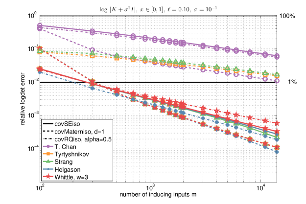
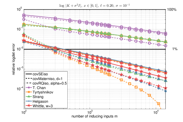
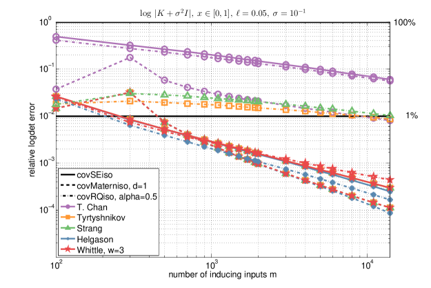
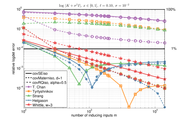
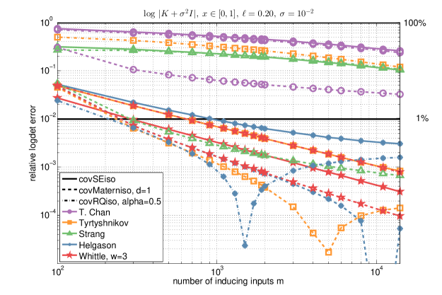
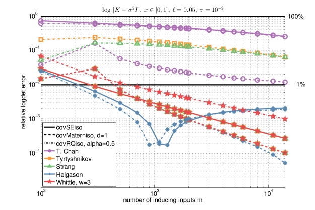
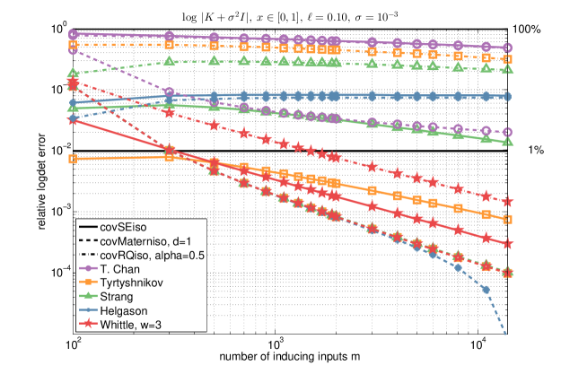
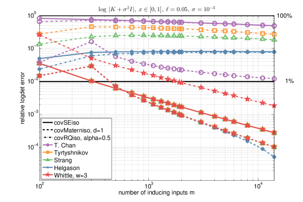
To speed up LCG for solving linear Toeplitz systems, one can use circulant pre-conditioners which act as approximate inverses. One wishes to minimise the distance between the preconditioner and the Toeplitz matrix , . Three classical pre-conditioners include (Strang,, 1986), (Chan,, 1988), and (Tyrtyshnikov,, 1992).
A distinct line of research was explored more than 60 years ago in the context of statistical inference over spatial processes (Whittle,, 1954). The circulant Whittle approximation is given by truncating the sum
i.e. we retain only.
Positive definiteness of for the complete sum is guaranteed by construction (Guinness and Fuentes,, 2014, Section 2). For large lattices, the approach is often used due to its accuracy and favourable asymptotic properties such as consistency, efficiency and asymptotic normality (Lieberman et al.,, 2009). In fact, the circulant approximation is asymptotically equivalent to the initial covariance , see Gray, (2005, Lemma 4.5), hence the logdet approximation inevitably converges to the exact value.
We use
where we threshold . denotes a vector , is the conjugate transpose of the Fourier transform matrix. denotes one of the T. Chan, Tyrtyshnikov, Strang, Helgason or Whittle approximations.
The particular circulant approximation pursued can have a dramatic practical effect on performance. In an empirical comparison (partly shown in Figure 1), we verified that the Whittle approximations yields consistently accurate approximation results over several covariance functions , lengthscales and noise variances decaying with grid size and below relative error for .
5.3 BCCB Approximation for BTTB
There is a natural extension of the circulant approximation of section 5.2 to multivariate data. A translation invariant covariance function evaluated at data points organised on a regular grid of size result in a symmetric block-Toeplitz matrix with Toeplitz blocks (BTTB), which generalises Toeplitz matrices. Unlike with Kronecker methods, the factorisation of a covariance function is not required for this structure. Using a dimension-wise circulant embedding of size , fast MVMs can be accomplished using the multi-dimensional Fourier transformation by applying Fourier transformations along each dimension rendering fast inference using LCG feasible. Similarly, the Whittle approximation to the log-determinant can be generalised, where the truncated sum for is over terms instead of . As a result, the Whittle approximation to the covariance matrix is block-circulant with circulant blocks (BCCB). Fortunately, BCCB matrices have an eigendecomposition , where is the Whittle approximation to , and as defined before. Hence, all computational and approximation benefits from the Toeplitz case carry over to the BTTB case. As a result, exploiting the BTTB structure allows to efficiently deal with multivariate data without requiring a factorizing covariance function.
We note that blocks in the BTTB matrix need not be symmetric. Moreover, symmetric BCCB matrices – in contrast to symmetric BTTB matrices – are fully characterised by their first column.
5.4 Projections
Even if we do not exploit structure in , our framework in section 5 provides efficiency gains over conventional inducing point approaches, particularly for test time predictions. However, if we are to place onto a multidimensional (Cartesian product) grid so that has Kronecker structure, then the total number of inducing points (the cardinality of ) grows exponentially with the number of grid dimensions, limiting one to about five or fewer grid dimensions for practical applications. However, we need not limit the applicability of our approach to data inputs with input dimensions, even if we wish to exploit Kronecker structure in . Indeed, many inducing point approaches suffer from the curse of dimensionality, and input projections have provided an effective countermeasure (e.g., Snelson,, 2007).
We assume the dimensional data inputs , and inducing points which live in a lower dimensional space, , and are related through the mapping , where we wish to learn the parameters of the mapping in a supervised manner, through the Gaussian process marginal likelihood. Such a representation is highly general: any deep learning architecture , for example, will ordinarily project into a hidden layer which lives in a dimensional space.
We focus on the supervised learning of linear projections, , where . Our covariance functions effectively become , , . Starting from the RBF kernel, for example,
The resulting kernel generalises the RBF and ARD kernels, which respectively have spherical and diagonal covariance matrices, with a full covariance matrix , which allows for richer models (Vivarelli and Williams,, 1998). But in our context, this added flexibility has special meaning. Kronecker methods typically require a kernel which separates as a product across input dimensions (section 3.1). Here, we can capture sophisticated correlations between the different dimensions of the data inputs through the projection matrix , while preserving Kronecker structure in . Moreover, learning in a supervised manner, e.g., through the Gaussian porcess marginal likelihood, has immediate advantages over unsupervised dimensionality reduction of ; for example, if only a subset of the data inputs were used in producing the target values, this structure would not be detected by an unsupervised method such as PCA, but can be learned through . Thus in addition to the critical benefit of allowing for applications with dimensional data inputs, can also enrich the expressive power of our MSGP model.
The entries of become hyperparameters of the Gaussian process marginal likelihood of Eq. (3), and can be treated in exactly the same way as standard kernel hyperparameters such as length-scale. One can learn these parameters through marginal likelihood optimisation.
Computing the derivatives of the log marginal likelihood with respect to the projection matrix requires some care under the structured kernel interpolation approximation to the covariance matrix . We provide the mathematical details in the appendix A.
For practical reasons, one may wish to restrict to be orthonormal or have unit scaling. We discuss this further in section 6.2.
6 Experiments
In these preliminary experiments, we stress test MSGP in terms of training and prediction runtime, as well as accuracy, empirically verifying its scalability and predictive performance. We also demonstrate the consistency of the model in being able to learn supervised projections, for higher dimensional input spaces.
We compare to exact Gaussian processes, FITC (Snelson and Ghahramani,, 2006), Sparse Spectrum Gaussian Processes (SSGP) (Lázaro-Gredilla et al.,, 2010), the Big Data GP (BDGP) (Hensman et al.,, 2013), MSGP with Toeplitz (rather than circulant) methods, and MSGP not using the new scalable approach for test predictions (scalable test predictions are described in section 5).
The experiments were executed on a workstation with Intel i7-4770 CPU and 32 GB RAM. We used a step length of for BDGP based on the values reported by Hensman et al., (2013) and a batchsize of . We also evaluated BDGP with a larger batchsize of but found that the results are qualititively similar. We stopped the stochastic optimization in BDGP when the log-likelihood did not improve at least by within the last steps or after iterations.
6.1 Stress tests
One cannot exploit Kronecker structure in one dimensional inputs for scalability, and Toeplitz methods, which apply to 1D inputs, are traditionally limited to about points if one requires many marginal likelihood evaluations for kernel learning. Thus to stress test the value of the circulant approximation most transparently, and to give the greatest advantage to alternative approaches in terms of scalability with number of inducing points , we initially stress test in a 1D input space, before moving onto higher dimensional problems.
In particular, we sample 1D inputs uniform randomly in , so that the data inputs have no grid structure. We then generate out of class ground truth data with additive Gaussian noise to form . We distribute inducing points on a regularly spaced grid in .
In Figure 2 we show the runtime for a marginal likelihood evaluation as a function of training points , and number inducing points . MSGP quickly overtakes the alternatives as increases past this point. Moreover, the runtimes for MSGP with different numbers of inducing points converge quickly with increases in . By , MSGP requires the same training time for inducing points as it does for inducing points! Indeed, MSGP is able to accommodate an unprecedented number of inducing points, overtaking the alternatives, which are using inducing points, when using inducing points. Such an exceptionally large number of inducing points allows for near-exact accuracy, and the ability to retain model structure necessary for large scale kernel learning. Note that inducing points (resp. basis functions) is a practical upper limit in alternative approaches (Hensman et al., (2013), for example, gives as a practical upper bound for conventional inducing approaches for large ).
We emphasize that although the stochastic optimization of the BDGP can take some time to converge, the ability to use mini-batches for jointly optimizing the variational parameters and the GP hyper parameters, as part of a principled framework, makes BDGP highly scalable. Indeed, the methodology in MSGP and BDGP are complementary and could be combined for a particularly scalable Gaussian process framework.
In Figure 3, we show that the prediction runtime for MSGP is practically independent of both and , and for any fixed is much faster than the alternatives, which depend at least quadratically on and . We also see that the local interpolation strategy for test predictions, introduced in section 5.1, greatly improves upon MSGP using the exact predictive distributions while exploiting Kronecker and Toeplitz algebra.
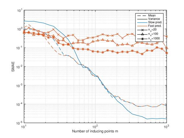
In Figure 4, we evaluate the accuracy of the fast mean and variance test predictions in section 5.1, using the same data as in the runtime stress tests. We compare the relative mean absolute error, , where are the true test targets, and is the mean of the true test targets, for the test predictions made by each method. We compare the predictive mean and variance of the fast predictions with MSGP using the standard (‘slow’) predictive equations and Kronecker algebra, and the predictions made using an exact Gaussian process.
As we increase the number of inducing points the quality of predictions are improved, as we expect. The fast predictive variances, based on local kernel interpolation, are not as sensitive to the number of inducing points as the alternatives, but nonetheless have reasonable performance. We also see that the the fast predictive variances are improved by having an increasing number of samples in the stochastic estimator of section 5.1.2, which is most noticeable for larger values numbers of inducing points . Notably, the fast predictive mean, based on local interpolation, is essentially indistinguishable from the predictive mean (‘slow’) using the standard GP predictive equations without interpolation. Overall, the error of the fast predictions is much less than the average variability in the data.
6.2 Projections
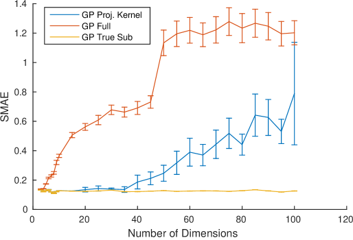
Here we test the consistency of our approach in section 5.4 for recovering ground truth projections, and providing accurate predictions, on dimensional input spaces.
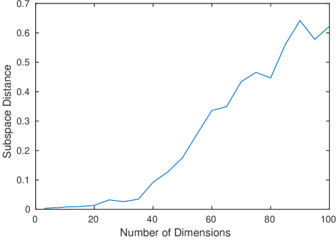
To generate data, we begin by sampling the entries of a projection matrix from a standard Gaussian distribution, and then project inputs (of dimensionality ), with locations randomly sampled from a Gaussian distribution so that there is no input grid structure, into a dimensional space: . We then sample data from a Gaussian process with an RBF kernel operating on the low dimensional inputs . We repeat this process times for each of .
We now index the data by the high dimensional inputs and attempt to reconstruct the true low dimensional subspace described by . We learn the entries of jointly with covariance parameters through marginal likelihood optimisation (Eq. (3)). Using a Cartesian product grid for total inducing points , we reconstruct the projection matrix , with the subspace error,
| (13) |
shown in Figure 5. Here is the orthogonal projection onto the -dimensional subspace spanned by the rows of . This metric is motivated by the one-to-one correspondence between subspaces and orthogonal projections. It is bounded in , where the maximum distance indicates that the subspaces are orthogonal to each other and the minimum is achieved if the subspaces are identical. More information on this metric including how to compute dist of Eq. (13) is available in chapter 2.5.3 of Golub and Van Loan, (2012).
We also make predictions on withheld test points, and compare i) our method using (GP Proj. Kernel), ii) an exact GP on the high dimensional space (GP Full), and iii) an exact GP on the true subspace (GP True), with results shown in Figure 5. We average our results times for each value of , and show standard errors. The extremely low subspace and SMAE errors up to validate the consistency of our approach for reconstructing a ground truth projection. Moreover, we see that our approach is competitive in SMAE (as defined in the previous section) with the best possible method, GP true, up to about . Moreover, although the subspace error is moderate for , we are still able to substantially outperform the standard baseline, an exact GP applied to the observed inputs .
We implement variants of our approach where is constrained to be 1) orthonormal, 2) to have unit scaling, e.g., . Such constraints prevent degeneracies between and kernel hyperparameters from causing practical issues, such as length-scales growing to large values to shrink the marginal likelihood log determinant complexity penalty, and then re-scaling to leave the marginal likelihood model fit term unaffected. In practice we found that unit scaling was sufficient to avoid such issues, and thus preferable to orthonormal , which are more constrained.
7 Discussion
We introduce massively scalable Gaussian processes (MSGP), which significantly extend KISS-GP, inducing point, and structure exploiting approaches, for: (1) test predictions (section 5.1); (2) circulant log determinant approximations which (i) unify Toeplitz and Kronecker structure; (ii) enable extremely fast marginal likelihood evaluations (section 5.2); and (iii) extend KISS-GP and Toeplitz methods for scalable kernel learning in D=1 input dimensions, where one cannot exploit multidimensional Kronecker structure for scalability. (3) more general BTTB structure, which enables fast exact multidimensional inference without requiring Kronecker (tensor) decompositions (section 5.3); and, (4) projections which enable KISS-GP to be used with structure exploiting approaches for input dimensions, and increase the expressive power of covariance functions (section 5.4).
We demonstrate these advantages, comparing to state of the art alternatives. In particular, we show MSGP is exceptionally scalable in terms of training points , inducing points , and number of testing points. The ability to handle large will prove important for retaining accuracy in scalable Gaussian process methods, and in enabling large scale kernel learning.
This document serves to report substantial developments regarding the SKI and KISS-GP frameworks introduced in Wilson and Nickisch, (2015).
References
- Chan, (1988) Chan, T. F. (1988). An optimal circulant preconditioner for Toeplitz systems. SIAM Journal on Scientific and Statistical Computation, 9(4):766–771.
- Cunningham et al., (2008) Cunningham, J. P., Shenoy, K. V., and Sahani, M. (2008). Fast Gaussian process methods for point process intensity estimation. In International Conference on Machine Learning.
- Deisenroth and Ng, (2015) Deisenroth, M. P. and Ng, J. W. (2015). Distributed gaussian processes. In International Conference on Machine Learning.
- Golub and Van Loan, (2012) Golub, G. H. and Van Loan, C. F. (2012). Matrix computations, volume 3. JHU Press.
- Gray, (2005) Gray, R. M. (2005). Toeplitz and circulant matrices: A review. Communications and Information Theory, 2.(3):155–239.
- Guinness and Fuentes, (2014) Guinness, J. and Fuentes, M. (2014). Circulant embedding of approximate covariances for inference from Gaussian data on large lattices. under review.
- Hensman et al., (2013) Hensman, J., Fusi, N., and Lawrence, N. (2013). Gaussian processes for big data. In Uncertainty in Artificial Intelligence (UAI). AUAI Press.
- Keys, (1981) Keys, R. G. (1981). Cubic convolution interpolation for digital image processing. IEEE Transactions on Acoustics, Speech and Signal Processing, 29(6):1153–1160.
- Lázaro-Gredilla et al., (2010) Lázaro-Gredilla, M., Quiñonero-Candela, J., Rasmussen, C., and Figueiras-Vidal, A. (2010). Sparse spectrum Gaussian process regression. The Journal of Machine Learning Research, 11:1865–1881.
- Le et al., (2013) Le, Q., Sarlos, T., and Smola, A. (2013). Fastfood-computing Hilbert space expansions in loglinear time. In Proceedings of the 30th International Conference on Machine Learning, pages 244–252.
- Lieberman et al., (2009) Lieberman, O., Rosemarin, R., and Rousseau, J. (2009). Asymptotic theory for maximum likelihood estimation in stationary fractional Gaussian processes, under short-, long- and intermediate memory. In Econometric Society European Meeting.
- Papandreou and Yuille, (2011) Papandreou, G. and Yuille, A. L. (2011). Efficient variational inference in large-scale Bayesian compressed sensing. In Proc. IEEE Workshop on Information Theory in Computer Vision and Pattern Recognition (in conjunction with ICCV-11), pages 1332–1339.
- (13) Quiñonero-Candela, J. and Rasmussen, C. (2005a). A unifying view of sparse approximate gaussian process regression. The Journal of Machine Learning Research, 6:1939–1959.
- (14) Quiñonero-Candela, J. and Rasmussen, C. E. (2005b). A unifying view of sparse approximate Gaussian process regression. Journal of Machine Learning Research (JMLR), 6:1939–1959.
- Rahimi and Recht, (2007) Rahimi, A. and Recht, B. (2007). Random features for large-scale kernel machines. In Neural Information Processing Systems.
- Rasmussen and Nickisch, (2010) Rasmussen, C. E. and Nickisch, H. (2010). Gaussian processes for machine learning (GPML) toolbox. Journal of Machine Learning Research (JMLR), 11:3011–3015.
- Rasmussen and Williams, (2006) Rasmussen, C. E. and Williams, C. K. I. (2006). Gaussian processes for Machine Learning. The MIT Press.
- Saatchi, (2011) Saatchi, Y. (2011). Scalable Inference for Structured Gaussian Process Models. PhD thesis, University of Cambridge.
- Snelson, (2007) Snelson, E. (2007). Flexible and efficient Gaussian process models for machine learning. PhD thesis, University College London.
- Snelson and Ghahramani, (2006) Snelson, E. and Ghahramani, Z. (2006). Sparse Gaussian processes using pseudo-inputs. In Advances in neural information processing systems (NIPS), volume 18, page 1257. MIT Press.
- Storkey, (1999) Storkey, A. (1999). Truncated covariance matrices and Toeplitz methods in Gaussian processes. In ICANN.
- Strang, (1986) Strang, G. (1986). A proposal for Toeplitz matrix calculations. Studies in Applied Mathematics, 74(2):171–176.
- Tyrtyshnikov, (1992) Tyrtyshnikov, E. (1992). Optimal and superoptimal circulant preconditioners. SIAM Journal on Matrix Analysis and Applications, 13(2):459–473.
- Vivarelli and Williams, (1998) Vivarelli, F. and Williams, C. K. (1998). Discovering hidden features with gaussian processes regression. Advances in Neural Information Processing Systems, pages 613–619.
- Whittle, (1954) Whittle, P. (1954). On stationary processes in the plane. Biometrika, 41(3/4):434–449.
- Williams and Seeger, (2001) Williams, C. and Seeger, M. (2001). Using the Nyström method to speed up kernel machines. In Advances in Neural Information Processing Systems, pages 682–688. MIT Press.
- Wilson, (2014) Wilson, A. G. (2014). Covariance kernels for fast automatic pattern discovery and extrapolation with Gaussian processes. PhD thesis, University of Cambridge.
- Wilson et al., (2014) Wilson, A. G., Gilboa, E., Nehorai, A., and Cunningham, J. P. (2014). Fast kernel learning for multidimensional pattern extrapolation. In Advances in Neural Information Processing Systems.
- Wilson and Nickisch, (2015) Wilson, A. G. and Nickisch, H. (2015). Kernel interpolation for scalable structured Gaussian processes (KISS-GP). International Conference on Machine Learning (ICML).
- Yang et al., (2015) Yang, Z., Smola, A. J., Song, L., and Wilson, A. G. (2015). A la carte - learning fast kernels. Artificial Intelligence and Statistics.
- Zhang et al., (2005) Zhang, Y., Leithead, W. E., and Leith, D. J. (2005). Time-series Gaussian process regression based on Toeplitz computation of operations and -level storage. In Proceedings of the 44th IEEE Conference on Decision and Control.
Appendix A APPENDIX
A.1 Derivatives For Normal Projections
-
•
apply chain rule to obtain from from
-
•
the orthonormal projection matrix is defined by , so that
A.2 Derivatives For Orthonormal Projections
-
•
the orthonormal projection matrix is defined by so that
-
•
apply chain rule to obtain from from
-
•
use eigenvalue decomposition , define ,
-
•
division in is component-wise
A.3 Circulant Determinant Approximation Benchmark