Abstract

On-line social networks publish information on a high volume of real-world events almost instantly, becoming a primary source for breaking news. Some of these real-world events can end up having a very strong impact on on-line social networks. The effect of such events can be analyzed from several perspectives, one of them being the intensity and characteristics of the collective activity that it produces in the social platform.

We research 5,234 real-world news events encompassing 43 million messages discussed on the Twitter microblogging service for approximately 1 year. We show empirically that exogenous news events naturally create collective patterns of bursty behavior in combination with long periods of inactivity in the network. This type of behavior agrees with other patterns previously observed in other types of natural collective phenomena, as well as in individual human communications. In addition, we propose a methodology to classify news events according to the different levels of intensity in activity that they produce. In particular, we analyze the most highly active events and observe a consistent and strikingly different collective reaction from users when they are exposed to such events. This reaction is independent of an event’s reach and scope. We further observe that extremely high-activity events have characteristics that are quite distinguishable at the beginning stages of their outbreak. This allows us to predict with high precision, the top 8% of events that will have the most impact in the social network by just using the first 5% of the information of an event’s lifetime evolution. This strongly implies that high-activity events are naturally prioritized collectively by the social network, engaging users early on, way before they are brought to the mainstream audience.

Introduction

Social media is now a primary source of breaking news information for millions of users all over the world  [?]. On-line social networks along with mobile internet devices have crowdsourced the task of disseminating real-time information. As a result, both news media and news consumers have become inundated with much more information than they can process. One possible way of handling this data overload, is to find ways to filter and prioritize information that has the potential of creating a strong collective impact. Understanding and quickly identifying the type of reaction that certain exogenous events will produce in on-line social networks, at both global and local scales, can help in the understanding of collective human behavior, as well as improve information delivery, journalistic coverage and crisis management, among other things. We address this challenge by analyzing the properties of real-world news events in on-line social networks, showing that they corroborate patterns previously identified in other case studies of human communications. In addition, we present our main findings of how news events that produce extremely high-activity can be clearly identified in the early stages of their outbreak.

The study of information propagation on the Web has sparked tremendous interest in recent years. Current literature on the subject primarily considers the process through which a meme, usually a piece of media (like a video, an image, or a specific Web article), gains popularity  [?,?,?,?,?,?,?,?]. However, a meme represents a simple information unit and its propagation behavior does not necessarily correspond to that of more complex information such as news events. News events are usually diffused in the network in many different formats, e.g., a particular news story such as an earthquake in Japan can be communicated through images, URLs, tweets, videos, etc. Therefore, current research can benefit from analyzing the effects of more high-level forms of information.

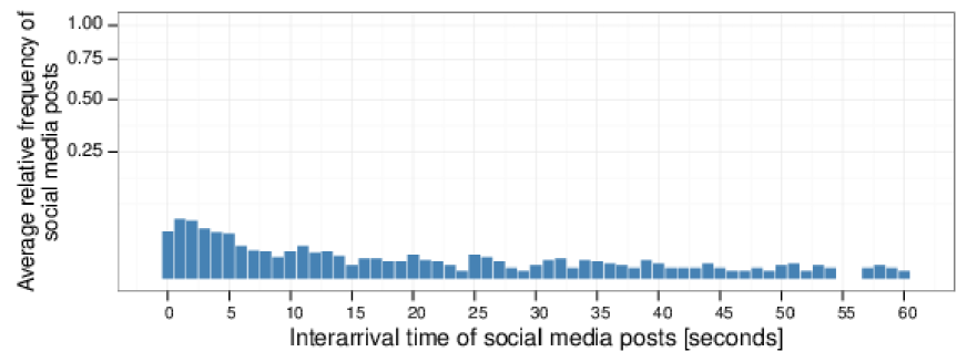
Traditionally, the impact of information in on-line social networks has been measured in relation to the total amount of attention that this subject receives  [?,?,?,?,?]. That is, if a content posted in the network receives votes/comments/shares above a certain threshold it is usually deemed as viral or popular. Nevertheless, this notion of popularity or impact will favor only information that produces very large volumes of social media messages. Naturally, global breaking news that has world-wide coverage and that produces a high volume of activity in a short time should be considered as having a strong impact on the network. However, there are other types of events that can produce a similar reaction in smaller on-line communities such as, for example, on users from a particular country (e.g., the withdrawal of the main right wing presidential candidate in Chile due to psychiatric problems, just before elections  [?]). Clearly, events of local scope do not produce as much social media activity as events of global scope, but they can create a strong and immediate reaction from users in local networks  [?]. Conversely, there are large events which do not produce an intense reaction, such as The Oscars (Fig. 1(b)), which span a long period of time and are discussed by social network users for weeks or even months, but do not spark intense user activity. Therefore, it is reasonable to consider additional dimensions, than just volume, when analyzing the impact of information in on-line communities.

Prior research has shown that certain types of individual activities, such as communications (studied in email exchanges), work patterns and entertainment, follow a behavior of bursts of rapidly occurring actions followed by long periods of inactivity  [?], referred to as temporally inhomogeneous behavior  [?]. This type of behavior initially observed in individual activities, has also been observed in relation to other naturally occurring types of collective phenomena in human dynamics similar to processes seen in self-organized criticality  [?]. In particular, extremely high-activity bursty behavior seems to also occur in critical situations, observed from the information flow in cell phone networks during emergencies [?]. Although, there is research towards modeling this type of collective behavior  [?] in on-line social networks, to the best of our knowledge, it has not yet been analyzed quantitatively.

Our work focuses on high-activity events in social media produced by real-world news, with the following contributions:

1. We introduce a methodology for modeling and classifying events in social media, based on the intensity of the activity that they produce. This methodology is independent of the size and scope of the event, and is an indicator of the impact that the event information had on the social network.

2. We show empirically that real-world news events produce collective patterns of bursty behavior in the social network, in combination with long periods of inactivity. Furthermore, we identify events for which most of their activity is concentrated into very high-activity periods, we call these events high-activity events.

3. We determine the existence of unique characteristics that differentiate how high-activity events propagate in the social network.

4. We show that an important portion of high-activity events can be predicted very early in their lifecycle, indicating that this type of information is spontaneously identified and filtered collectively, early on, by social network users.

Materials and Methods

We define an event as a conglomerate of information that encompasses all of the social media content related to a real-world news occurrence. Using this specification, which considers an event as a complex unit of information, we study the type of collective reaction produced by the event on the social network. In particular, we analyze the intensity or immediacy of the social network’s response. By analyzing the levels of intensity in activity induced by different exogenous events to the network, we are implicitly studying the priority that has been collectively assigned to the event by groups of independent individuals  [?,?].

We characterize an event’s discrete activity dynamics by using interarrival times between consecutive social media messages within an event (e.g., $d_{i}=t_{i+1}-t_{i}$, where $d_{i}$ denotes the interarrival time between two consecutive social media messages $i$ and $i+1$ that arrived in moments $t_{i}$ and $t_{i+1}$, respectively).

We introduce a novel vectorial representation based on a vector quantization of the interarrival time distribution, which we call “VQ-event model”. This model is designed to filter events based on the distribution of the interarrival times between consecutive messages. This approach is inspired by the codebook-based representation from the field of multimedia content analysis, which has been used in audio processing and computer vision   [?,?]. In our proposed approach, our method learns a set of the most representative interarrival times from a large training corpus of events; each one of the representative interarrival times is known as a codeword and the complete learned set is known as the codebook  [?]. Each event is then modeled using a vector quantization (VQ) that converts the interarrival times of an event into a discrete set of values, each value corresponding to the closest codeword in the codebook (details in supplementary material). The resulting VQ-event model is then a vector in which each dimension contains the percentage of interarrival times of the event that were assigned a particular codeword in the codebook.

The VQ-event representation is relative to an event’s overall size since the model is normalized with respect to the number of messages in the event. Therefore the only criteria that are considered in the model are the interarrival times of each particular event. This model allows us to group events based on the similarity of the distribution of their interarrival times. In those terms, we consider as high-activity events those events for which the distribution of interarrival times is most heavily skewed towards the smallest possible interval, zero. In other words, events for which the overall activity is extremely intense in comparison with other events.

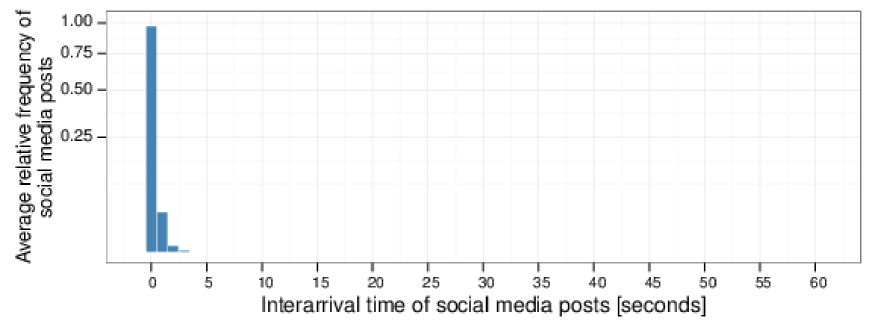
To illustrate events with different levels of intensity in activity we present two examples taken from our analysis of Twitter data. These examples show the interarrival time histograms for the entire lifecycle of the two events. In the first example, the majority of the messages about the death of political leader Nelson Mandela (Fig. 1(a)) arrive within almost zero seconds of each other. On the contrary, the messages about The Oscars (Fig. 1(b)) are much more spread out in time.

(a) User posts about the death of Nelson Mandela arrive almost instantly.

(b) User posts about The Oscars arriving several weeks before the event.

Figure 1: Examples of interarrival time histograms of two real-world news events discussed on Twitter. The event [nelson, mandela] (1(a)) was collected on 12/05/2013. Since there is a high concentration in the first histogram bin, we conclude that most of the social media posts for this event occur in one or more successions of high-activity bursts (therefore, considered a high-activity event). The second event, [may, oscar] (1(b)) was collected on 03/23/2014 about The Oscars event that was held a few weeks before. The arrival times of these posts are much more spread out, displaying much less concentration of bursty activity.

We note that, by using interarrival times to describe the intensity of the activity of an event, we make our analysis independent of the particular evolution of each event. By doing this, we put no restrictions on how high-activity events unfold in time, for example, they could be: (a) events that start out slowly and suddenly gain momentum, (b) events that go viral soon after they appear on social media and then decay in intensity over a long (or short) period of time, (c) events that from the beginning produce large amounts of interest and sustain that interest throughout their long (or short) lifespan, or (d) events that are a concatenation of any of the above, etc.

We study a dataset of news events gathered from news headlines from a manually curated list of well-known news media accounts (e.g., @CNN, @BreakingNews, @BBCNews, etc.) in the microblogging platform Twitter  [?] (a full list of all the news media accounts is provided in the supplementary material). Headlines were collected periodically every hour, over the course of approximately one year. In parallel, all the Twitter messages (called tweets) were extracted for each news event using the public API  [?]. This process was performed by automatically extracting descriptive sets of keywords for each event using a variation of frequent itemset extraction  [?] over the event’s headlines. These sets of keywords were then used to retrieve corresponding user tweets for each event. We validate the events gathered in our data collection process to ensure that each group of social media posts corresponds to a meaningful and cohesive news event. We provide a detailed description of the collection methodology and of the validation of event cohesiveness in the supplementary material. Overall, the resulting dataset contains $43,256,261$ tweets that account for $5,234$ events (Table 6).

In Figure 2 we characterize an example event from our dataset, by showing the set of keywords and a sample of tweets associated to the event. These keywords form a semantically meaningful event; they refer to the incident where soccer player Luis Suarez was charged for biting another player during the FIFA World Cup in 2014. This general collection process results in a set of social media posts associated to an event which can encompass several memes, viral tweets and pieces of information. Therefore, an event is composed of diverse information, addressing more heterogeneous content than prior work  [?,?,?,?,?,?,?] which focus on single pieces of information (e.g., a particular meme, a viral tweet etc.).

Event Collection Statistics	Minimum	Mean	Median	Maximum
# of posts (per event)	1,000	8,254	2,474	510,920
# of keywords (per tweet)	2	3.77	3	39
Event duration (hours)	0.12	20.93	7.46	190.43

Table 1: High-level description of the dataset of news events.

Figure 2: An example event, collected on 06/25/2014 with keywords (left) and sample user posts (right) obtained from the Twitter Search API. The tweets in the event contain at least a pair of descriptive keywords and were retrieved close to the time of the event.

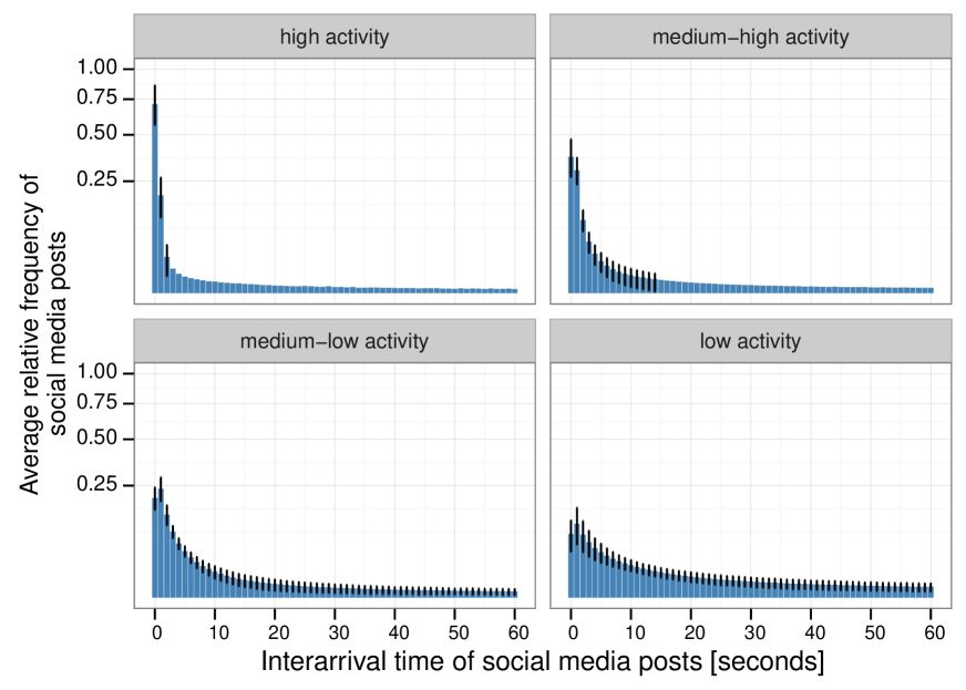
The collection of events is converted into their VQ-event model representation. Using this model, we can identify events that have produced similar levels of activity in the social network. In other words, events are considered to have similar activity if the interarrival times between their social media posts are similarly distributed, implying a very much alike collective reaction from users to the events within a group. In order to identify groups of similar events, we cluster the event models. We sort the resulting groups of events from highest to lowest activity, according to the concentration of social media posts in the bins that correspond to short interarrival times. We consider the events that fall in the top cluster to be high-activity events as most of their interarrival times are concentrated in the smallest interval of the VQ-event model. In our dataset, these correspond to roughly 8% of the events. We consider the next clusters in the sorted ranking to form medium-high activity events, and so on. Thus we end with four groups of events: high, medium-high, medium-low and low. Figure 3 shows a heatmap of the interarrival relative frequency for each cluster. This classification of events based on activity intensity is independent of event size. More details of this methodology are provided in the supplementary material.

Figure 3: Each row is the average representation of all the events in a cluster. A darker cell represents a higher relative frequency value. The y-axis specifies the number of events in each cluster. Clusters are (top to bottom): high-activity, medium-high medium-low and low.

Results and Discussion

Our main objective in this work is to analyze the characteristics of high-activity events which differentiate them from other types of events. In particular, we identify how early on in an event’s lifecycle can we determine if an event is going produce high activity in the on-line social network.

Tables Results and Discussion and Results and Discussion show examples of events from the high-activity category and low-activity category. We recall that the high-activity events are those which were in the top 8% of the ranking obtained by sorting the event clusters according to concentration of interarrival times of social media posts in the shortest interarrival time of the VQ-event model. Table Results and Discussion shows two events of different sizes (large and small) and different scopes (one global and the other of more local scope) categorized as high activity in our dataset. The first event, the death of Nelson Mandela, is one of the largest events in the dataset, with $\approx 134,000$ tweets. The histogram representation of this event, shown in Figure 1(a), suggests that more than $80\%$ of the activity of the event was produced in high-activity periods. This is an event of international, political, and social importance, that produced an overwhelming flood of messages on social media. Hence, it makes sense for such an example to be a high-activity event. The second event, on the other hand, about the 2013 Mumbai Gang Rape is of much smaller scale, with a total of $\approx 1,700$ tweets. However, this event caused considerable amount of immediate reaction on social media, with close to $50\%$ of its activity concentrated within high-activity periods. Despite its smaller size, in comparison to the previous event, this event displays a similar reaction to that of other high-activity events, but at a smaller scale.

Table Results and Discussion shows events that have been classified by our methodology in the category of low activity. The first event, about a teen surviving after hiding in the wheel of a airplane, had only a little more than $25\%$ of its messages arriving with high-activity bursts although it had over $18,000$ messages. The second event, about the damages caused by a tornado in Canada, did not garner much immediacy in attention of Twitter users, with only $7\%$ of its messages produced with short interarrival times. Most of the messages of this event were well spaced out in time. Even though we cannot say whether or not this event had significant implications in the real-world, we can say that it did not have considerable impact on the Twitter network. The lack of interest could be due to several factors that are currently beyond the scope of this work, ranging from the lack of Twitter users in the locality of the real-world event, to it not being considered urgent by Twitter users. We intend to research the relation between the real-world impact of an event and the network reaction in future work.

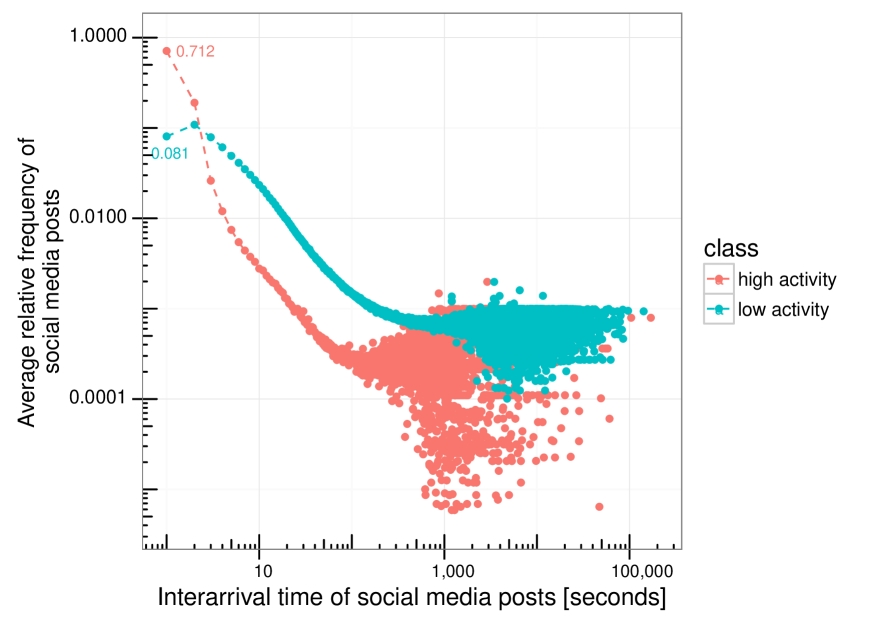
Fig. 4 shows the average histograms for events that belong to the high activity, medium-high activity, medium-low activity and low-activity clusters (displayed from left to right and top to bottom). All histograms show a quick decay in average relative frequency (resembling a distribution from the exponential family). In particular, the high-activity group concentrates most of its activity in the shortest interarrival rate, with lower activity groups mostly concentrating their activity in the second bin with slower decay. Fig. 5 further characterizes the differences in behavior of the high and low-activity groups, showing that high-activity events concentrate on average $70\%$ fo their activity in the smallest bin ($0$ sec.), against $8\%$ for low-activity events. In addition, Fig. 6 (left) shows the cumulative distribution function (CDF) for each group of events, and Fig. 6 (right) shows $\log{(1-\mathrm{CDF})}$. Visual inspection shows a clear difference in how interarrival rates are distributed within each group, however, these figures do not indicate a power-law distribution nor exponential distribution.

Event	Sample Tweets
20cmDescription:
Death of South African
politician Nelson Mandela.
Keywords:
[nelson, mandela]
Date:
2013-12-05
Size:
134,637 tweets	20cm @DaniellePeazer: RIP Nelson Mandela….. what a truly phenomenal and
inspirational man xx
@iansomerhalder: Im in tears.The world has lost one of its greatest shepherds
of peace. Thank you Mr.Mandela for the love you radiated. http://t.co/u39MVVEKe8
@FootballFunnys: This is so true. RIP Nelson Mandela. http://t.co/vF9xri8LdP
@David_Cameron: I’ve spoken to the Speaker and there will be statements
and tributes to Nelson Mandela in the House on Monday.
20cmDescription:
2013 Mumbai Gang Rape
Keywords:
[rape, mumbai]
Date:
2013-08-24
Size:
1,705 tweets	20cm @TheNewsRoundup: Mumbai gang-rape: Second accused confesses to crime:
Mumbai Police - Daily News Analysis http://t.co/KnabwhqH66
@vijayarumugam: An interesting take on the Mumbai rape: http://t.co/ylBmW4l8sA
@LondonStephanie: Two arrested over gang rape of Mumbai photojournalist
that sparked renewed protests in India http://t.co/McYfLNDvaE
@GanapathyI: Most brutal rapist of Delhi gang-rape was 17. Most brutal rapist
of Mumbai gang-rape is 18. Worst Young generation I have seen in my life.

Table 2: Examples of high-activity news events. The events shown were taken from the “high” category according to Fig. 4.

20cmDescription: Surveying the damages of recent tornado in Canada. Keywords: [canada, tornado] Date: 2014-06-21 Size: 1,033 20cm @Kathleen_Wynne: Visited #Angus today to survey the damage. Thankfully no fatalities or major injuries from recent tornado. http://t.co/xRQyRWg5Vw @SunNewsNetwork: PHOTOS & VIDEO: Hundreds displaced after tornado hits Ontario town, destroying homes http://t.co/L38rG6N1a6 @CBCToronto: Kathleen Wynne is speaking at site of tornado damage in Angus, Ont. now. Watch live here: http://t.co/EDKNUiZo0X #cbcto @InsuranceBureau: @CTVBarrieNews: Insurance Bureau of Canada is setting up a mobile unit in #Angus today to help residents affected by #Tornado

Table 3: Examples of events with low activity. The events shown were taken from the “low” category according to Fig. 4 .

Figure 4: Average histograms of the high activity, medium-high activity, medium-low activity and low activity clusters in our dataset (from left to right and top to bottom). All histograms include standard deviation bars and were cut-off at 60 second length for better visibility.

Figure 5: Scatter plots of the average relative frequencies of interarrival times for the high-activity and low-activity clusters of events (i.e., scatter plots of the histograms in Fig. 4 in log-log scale). $y$-axis represents the average relative frequency of social media messages and $x$-axis the interarrival time.

Figure 6: (Left) Average cumulative distribution function (CDF) for the high activity, medium-high activity, medium-low activity and low activity clusters in our dataset. (Right) $\log{(1-\mathrm{CDF})}$ for the same clusters.

Further analysis of the high-activity events shows significant differences to other events, in the following aspects: (i) how the information about these events is propagated, (ii) the characteristics of the conversations that they generate, and (iii) how focused users are on the news topic. In detail, high-activity events have a higher fraction of retweets (or shares) relative to their overall message volume. On average, a tweet from a high-activity event is retweeted 2.36 times more than a tweet from a low activity event. The most retweeted message in high-activity events is retweeted 7 times more than the most retweeted message in a medium or low activity event. We find that a small set of initial social media posts are propagated quickly and extensively through the network without any rephrasing by the user (just plain forwarding). Intuitively, this seems justified given general topic urgency of high-activity events. Events that are not high-activity did not exhibit these characteristics.

Our research also revealed that high-activity events tend to spark more conversation between users, 33.4% more than other events. This is reflected in the number of replies to social media posts. The number of different users that engage with high-activity events is 32.7% higher than in events that are not high-activity. Posts about high-activity events are much more topic focused than in other events. The vocabulary of unique words as well as hashtags used in high-activity events is much more narrow than for other events. Medium and low activity events have over 7 times more unique hashtags than high-activity events. This is intuitive, given that if a news item is sensational, people will seldom deviate from the main conversation topic.

In a real-world scenario, in order to predict if an early breaking news story will have a considerable impact in the social network, we will not have enough data to create its activity-based model, i.e., we will not yet know the distribution of the speed at which the social media posts will arrive for the event. For instance, an event can start slowly and later produce an explosive reaction, or start explosively and decay quickly to an overall slower message arrival rate. Still, reliable early prediction of very high-activity news is important in many aspects, from decisions of mass media information coverage, to natural disaster management, brand and political image monitoring, and so on.

For the task of early prediction of high-activity events we use features that are independent of our activity-based model such as the retweets, the sentiment of the posts about the event, etc. These features are computed on the early 5% of messages about the event. The results are an average from a 5-fold cross validation with randomly selected 60% training, 20% validation and 20% test splits. The high-activity events are identified with a precision of 82% using only the earliest 5% of the data of each event (Table 13). Additionally, we were able to identify with high accuracy a considerable percentage of all high-activity events ($\approx 46\%$) at an early stage, with very few false positives (Table 13 and 12).

	Early 5% Tweets				All Tweets
	FP-Rate	Precision	Recall	ROC-area	FP-Rate	Precision	Recall	ROC-area
high-activity	0.009	0.819	0.455	0.900	0.01	0.830	0.540	0.945
non-high-activity	0.545	0.954	0.991	0.900	0.460	0.960	0.990	0.945

Table 4: Classification of high-activity events.

	Early 5% Tweets		All Tweets
	high-activity	non-high-activity	high-activity	non-high-activity
high-activity	$194$	$232$	$230$	$196$
non-high-activity	$43$	4,765	47	4,761

Table 5: Confusion matrix for high-activity events prediction.

The precision using only the early tweets is almost as good as using all tweets in the event (0.819 to 0.830). This suggests that the social network somehow acts as a natural filter in separating out the high-activity events fairly early on. The recall goes from 0.455 to 0.540. This indicates that there are some high-activity events which require more data in order to determine what kind of activity they will produce, or events for which activity occurs due to random conditions. A detailed description of the features and different classification settings are provided in the supplementary material.

Conclusion

We study the characteristics of the activity that real-world news produces in the Twitter social network. In particular, we propose to measure the impact of the real-world news event on the on-line social network by modeling the user activity related to the event using the distribution of their interarrival times between consecutive messages. In our research we observe that the activity triggered by real-world news events follows a similar pattern to that observed in other types of collective reactions to events. This is, by displaying periods of intense activity as well as long periods of inactivity. We further extend this analysis by identifying groups of events that produce much more concentration of high-activity than other events. We show that there are several specific properties that distinguish how high-activity events evolve in Twitter, when comparing them to other events. We design a model for events, based on the codebook approach, that allows us to do unambiguous classification of high-activity events based on the impact displayed by social network. Some notable characteristics of high-activity events are that they are forwarded more often by users, and generate a greater amount of conversation than other events. Social media posts from high-activity news events are much more focused on the news topic. Our experiments show that there are several properties that can suggest early on if an event will have high-activity on the on-line community. We can predict a high number of high-activity events before the network has shown any type of explosive reaction to them. This suggests that users are collectively quick at deciding whether an event should receive priority or not. However, there does exist a fraction of events which will create high activity, despite not presenting patterns of other high activity events during their early stages. These events are likely to be affected by other factors, such as random conditions found in the social network at the moment and require further investigation.

Supporting Information

S1 Appendix

1 Data Collection Methodology

The Twitter Search API was used to obtained tweets about $5,234$ news events. This encompasses a total of $43,256,261$ tweets. Table 6 shows a high level description of the dataset. The full dataset is available in http://dcc.uchile.cl/~mquezada/breakingnews/.

News events’ property	Minimum	Mean	Median	Maximum
# of tweets	$1,000$	$8,254$	$2,474$	$510,920$
# of keywords	$2$	$3.77$	$3$	$39$
Event duration (hours)	$0.12$	$20.93$	$7.46$	$190.43$

Table 6: High-level description of the dataset of news events.

1.1 Collecting the Tweets

The data collection process entails detecting pairs of keywords from the most recent hourly batch of news headlines (the pairs of keywords are meant to describe the events succinctly), and then searching for tweets using the pairs of keywords as queries. We merge the search results of ‘similar’ queries every 24 hours and form the tweets set for an event. We obtained the hourly batch of headlines from the news media accounts on Twitter listed in Table LABEL:table:acct_names. Figure 7 represents the high-level flowchart of the data collection process. A summary of this process is described in Algorithm 1. The accounts are verified accounts on Twitter.

Table 7: List of news account. The first column is the Twitter account. It can be accessed in a browser at http://twitter.com/accountname. The second and third columns were obtained from each account’s page.

Twitter Account	Name	Location
breakingnews	Breaking News	Global
cnnbrk	CNN Breaking News	Everywhere
cnn	CNN
nytimes	The New York Times	New York City
bbcbreaking	BBC Breaking News	London, UK
theeconomist	The Economist	London
skynewsbreak	Sky News Newsdesk	London, UK
reuters	Reuters Top News	Around the world
wsjbreakingnews	WSJ Breaking News	New York, NY
foxnews	Fox News	U.S.A.
msnbc_breaking	msnbc.com Breaking
skynews	Sky News	London, UK
nbcnews	NBC News	New York, NY
cbsnews	CBS News	New York, NY
bbcworld	BBC News (World)	London, UK
abc	ABC News	New York, NY
bbcnews	BBC News (UK)	London
ap	The Associated Press	Global
telegraphnews	Telegraph News	London, UK
breakingnewsuk	Breaking News UK	London
channel4news	Channel 4 News	Weekdays at 7 on Channel 4
twcbreaking	TWC Breaking	Atlanta, GA
washingtonpost	Washington Post	Washington, D.C.
yahoonews	Yahoo News	Santa Monica, Calif.
breakingpol	Breaking Politics	Global
nydailynews	New York Daily News	New York City
ajenglish	Al Jazeera English	Doha, Qatar
usatoday	USA TODAY	USA TODAY HQ, McLean, Va.
wsj	Wall Street Journal	New York, NY
guardiannews	Guardian news	London
bloombergnews	Bloomberg News	New York and the World
abcworldnews	ABC World News	New York
nypost	New York Post	New York, NY
msnbc	msnbc
nbcnightlynews	NBC Nightly News	New York
huffingtonpost	Huffington Post
rt_com	RT
abcnews	ABC News	Australia
latimes	Los Angeles Times	Los Angeles, CA
googlenews	Google News	Mountain View, CA
cnnlive	CNN Live	Everywhere
newshour	NewsHour	Arlington, VA
guardian	The Guardian	London
afp	Agence France-Presse	France
independent	The Independent	London, United Kingdom
ndtv	NDTV	India
cp24	CP24	Toronto
reuterslive	Reuters Live	Global
bostonglobe	The Boston Globe	Boston, MA
foxnewsalert	Fox News Alert	New York, NY
ft	Financial Times	London
jerusalem_post	The Jerusalem Post	Israel
bbcnewsus	BBC News US	Washington DC
foxheadlines	Fox News	New York, NY
forbes	Forbes	New York, NY
thetimes	The Times of London	London
usnews	U.S. News	Washington, DC

In Algorithm 1, the goal of the detect_keywords() module is to produce pairs of keywords that coherently, and succinctly describes an event. Inspired by the data mining concept of mining frequent itemsets  [?], we develop an algorithm which identifies the most commonly occurring keyword groups (or item sets) in the headlines. From the item sets, we pick the most common keyword pairs. The algorithm is described in Algorithm 2. This algorithm finds string intersections between headlines (intersect() in Line 5 returns the number of words present in both $s_{a}$ and $s_{b}$). If the common set of words has sufficient Jaccard similarity to any of the existing item sets, then the common set of words are added to that item set. If not, a new item set is created (Line 11). During the process of identifying the most commonly occurring item sets, we also track how many times each keyword has been added to an item set, namely, the score of the keyword. The score of each item set is the average of the scores of its keywords. Once the item sets have been identified, we select the top 2 keywords from each of the top six item sets and use them for searches. We preprocess the headlines to remove duplicates, stopwords, punctuation, convert everything to lower case, and subject the text through the process of stemming.

We made the choice of selecting 2 keywords since having a single keyword maybe not define an event accurately. For example, the keyword {obama} could retrieve tweets about any event related to Obama. However, a keyword pair like {obama, syria} describes the event more accurately.

The Twitter Search API imposes several restrictions on the number of searches that can be performed in a given time duration. We produce six search threads to perform searches, one for each keyword pair. All in all, with $\tau=60$ minutes in Figure 7, six new pairs of keywords are discovered from the most recent batch of headlines, and then we query for tweets in the Twitter Search API using these keywords over the next one hour.

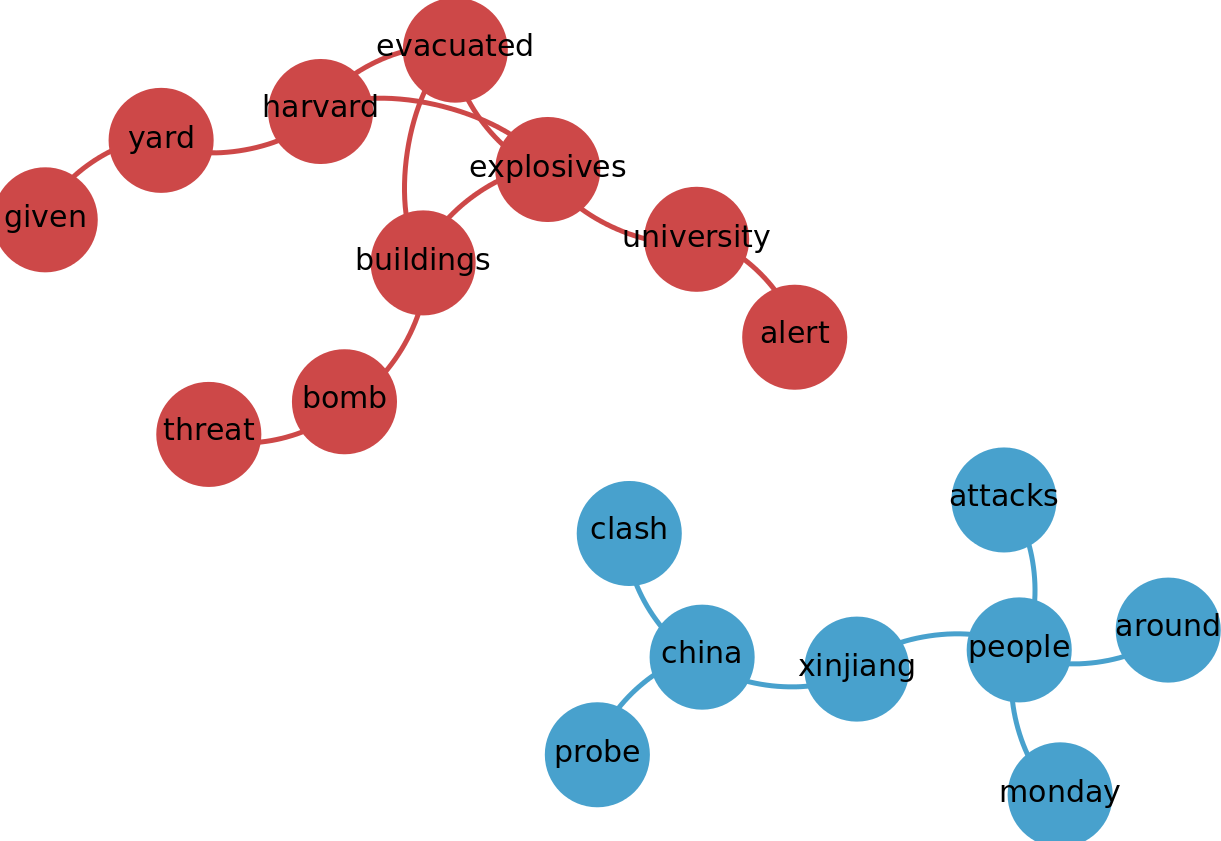
We make some notes about the data collection methodology. Firstly, there is a temporal sensitivity to the data collection methodology. For example, one of the keyword pairs obtained as soon the Malaysian airlines jet disappeared was {plane,missing}. Although this keyword pair does not specifically refer to the Malaysian airlines jet, it is likely that the tweets retrieved from searching for this pair will indeed be about the Malaysian airlines plane that went missing, since the search is performed as and when the event breaks out. Secondly, Algorithm 2 may return multiple pairs of keywords (possibly different pairs) describing the same event. Some pair examples of keywords produced when there was a bomb threat at Harvard University in December 2013 were {harvard, evacuated}, {harvard, explosives}, etc. How do we merge the keyword pairs which belong to the same event? In order to address this, we collect all the pairs obtained in the past $24$ hours, and build a graph with keywords as nodes, and keyword pairs (as obtained from Algorithm 2) as edges. We then discover the connected components of this graph, and treat each connected component as an “event”. The set of tweets obtained by merging the tweets from each of the keyword pairs is the set of messages associated with the event. Figure 10 is an example component formed on December 16, 2013. It illustrates the merge of smaller keyword pairs into larger components for two events. One was the bomb threat at Harvard University, and the other was about the attack on police in the Xinjiang province in China.

Figure 7: This figure illustrates the high level data collection process. Headlines are collected every hour, and $6$ keyword pairs are chosen to search for tweets. These keyword pairs are detected with the goal of concisely representing queries for an event.

Algorithm 1 data_collection()

0: stream of headlines.

0: data structures $\{\mathcal{H}_{1},\mathcal{H}_{2},\ldots\}$, with $\mathcal{H}.keywords$ = keyword pair, and $\mathcal{H}.tweets$ = set of tweets

1: $i\leftarrow 0$, $j\leftarrow 0$

2: loop

3:    $\mathcal{S}\leftarrow$ headlines for hour-$i$

4:    $keyPairs\leftarrow$ detect_keywords$(\mathcal{S})$ {$keyPairs$ is a list of keyword pairs.}

5:    for $k=0$ to len($keyPairs$)$-1$ do

6:       $\mathcal{H}_{j}.keywords\leftarrow keyPairs[k]$

7:       $\mathcal{H}_{j}.tweets\leftarrow$search$(\mathcal{H}_{j}.keywords)$ {using Twitter Search API}

8:       $j\leftarrow j+1$

9:    end for

10:    $i\leftarrow i+1$

11: end loop

Algorithm 2 detect_keywords()

0: A set of $M$ sets of words, $\mathcal{S}=\{H_{1},H_{2},\ldots,H_{M}\}$, positive integers $k,\eta$

0: $k$ sets of keywords, $G=(\mathcal{I}_{1},\mathcal{I}_{2},\ldots,\mathcal{I}_{k})$

1: $\mathcal{I}_{i}\leftarrow\emptyset$ for $i=1,2,\ldots,k$

2: $score_{i}\leftarrow$ empty dictionary for $i=1,2,\ldots,k$

3: $i\leftarrow 1$

4: for every pair of headlines $\{H_{a},H_{b}\}\in\mathcal{S}$ such that $|H_{a}\cap H_{b}|\geq\eta$ do

5:    $\mathcal{G}\leftarrow H_{a}\cap H_{b}$

6:    $j\leftarrow\operatorname{arg\,max}_{j}|\mathcal{I}_{j}\cap\mathcal{G}|$

7:    if $|\mathcal{I}_{j}\cap\mathcal{G}|\geq\eta$ then

8:       $\mathcal{I}_{j}\leftarrow\mathcal{I}_{j}\cap\mathcal{G}$

9:       $score_{j}[w]\leftarrow score_{j}[w]+1$ for all $w\in\mathcal{I}_{j}$

10:    else

11:       $\mathcal{I}_{i}\leftarrow\mathcal{G}$

12:       $score_{i}[w]\leftarrow 1$ for all $w\in\mathcal{I}_{i}$

13:       $i\leftarrow i+1$

14:    end if

15: end for

16: $total\_score_{i}\leftarrow\sum_{w\in\mathcal{I}_{i}}score_{i}[w]$ for $i=1,2,\ldots,k$

17: return  $G\leftarrow(\mathcal{I}_{i}$ sorted by $total\_score_{i})$

1.2 Cleaning the Data

The data was preprocessed to reduce the noisy and irrelevant tweets.

1.2.1 Special Stopwords: Articulation Words

During the data collection process, sometimes unrelated events were joined together with keywords that was common to both events.

Typical stopwords such as “the” and “a” were removed during preprocessing the news headlines. However, there are other words which occur quite commonly in news headlines. For example, words like “watch”, “live”, or “update” are common to express things like “watch this video”, “we are live on TV”, or to update a previous headline with more information. Such words could possibly incorrectly connect two or more very different events as one. Example: “Watch Jim Harbaugh’s press conference live” and “WATCH LIVE: Of the 48 people being monitored for contact with Dallas patient, no one is showing any symptoms”. We call such words articulation words We now delve into understanding how and when these words occur, and how to subsequently identify and remove them in the preprocessing step, just as we would a stopword.

It is well known that tf-idf  [?] is a statistic of a word that indicates how important that word is in a given document. Intuitively, if a word appears in all the documents, then its statistic is generally low in all the documents. However, if the word appears in very few documents, its statistic in those documents is fairly high, indicating that the word is somehow representative of the content of the document. It turns out the articulation words do not occur often enough for them to be detected by regular tf-idf, but do occur enough times for them to falsely relate several unrelated events together. To identify a group of those keywords, we used a modified tf-idf to detect them from the headlines.

The modified version of tf-idf, what we refer as maxtf-idf, is meant to assign more weight to the terms that are frequent in any document. For instance, tf-idf of a term in a document tries to assign a weight related to how “rare” that term is in the whole collection, and how frequent the term is in that document, thus indicating how representative the term is of the document. On the other hand, we want to place a higher weight on a term if its frequency is higher in any other document, relative to the frequency in the current document. With that in mind, we want to identify terms that might be “adding noise” to the corpus and hence merge unrelated events together.

The definition of maxtf is as follows:

$$\text{maxtf}(t,d,D)=0.5+\frac{0.5+max\{f(t,d^{\prime}):d^{\prime}\in D\}}{max\{f(w,d):w\in d\}}$$ (1)

and for idf, the usual formula:

$$\text{idf}(t,D)=\log\frac{N}{|\{d\in D:t\in d\}|}$$ (2)

where $t$ is a term, $d$ is a document, and $D$ is the corpus of all documents. In this case, we set $t$ as a keyword, $d$ as the set of keywords of one hour of a given day, and $D$ the set of documents of that day.

Figure 8: Stopwords detection. Normalized $1-\text{maxtf-idf}$ score for data from August 27th (left) and August 28th (right) of 2013. The top score words for both plots are “says” and “live”. We used the top score words to disconnect connected components of events.

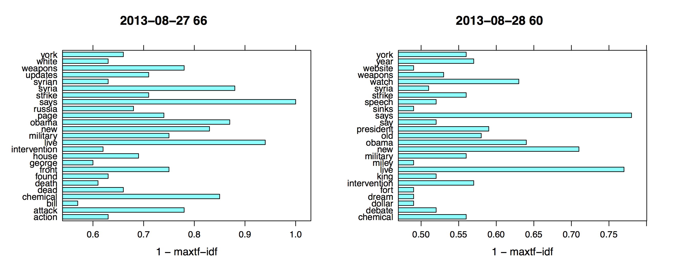
After identifying such words, the idea is to disconnect the components connected by those words. The process is to disconnect each component by the word with top normalized $1-\text{maxtf-idf}$ score each time until the component could not be disconnected further. We add the top scoring words to our list of stopwords. These words are hence ignored from the subsequent runs of the data collection methodology. In Figure 8 there are two examples of this process to identify the words.

1.2.2 Discarding Irrelevant Tweets

Due to the capabilities of the REST API, the tweets collected can be older than the actual date of the event detected. Hence, some tweets can be very old and not relevant to the event itself. This may lead to inaccuracies in predictions when using the early features.

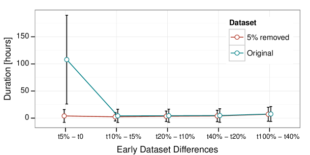
This problem is illustrated in Figure 9, Note that the first 5% of the tweets take an unusually large portion of the duration of the entire event. This suggests that we are collecting tweets which existed much before the event broke out, and hence are possibly irrelevant. Once we discard the first 5% of tweets, we observe that each segment of the event (first 5%, the next 5%, etc.) occupies roughly the same duration of the entire event.

Figure 9: Duration differences of events. The $x$-axis represents the categories of datasets: the first one (t5%-t0) represents the difference of time between the timestamp of the oldest tweet and the newest tweet in the first 5% of the tweets. The next one (t10%-t5%) corresponds to the difference between the newest tweet in the first 10% and the newest tweet in the first 5% of data, etc. After removing the first 5% of data, the time differences are roughly the same across all datasets.

1.3 Validation of Data Collection

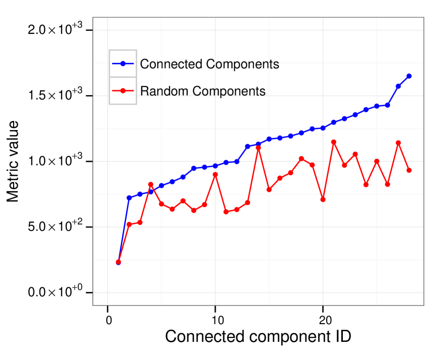
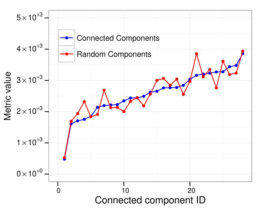
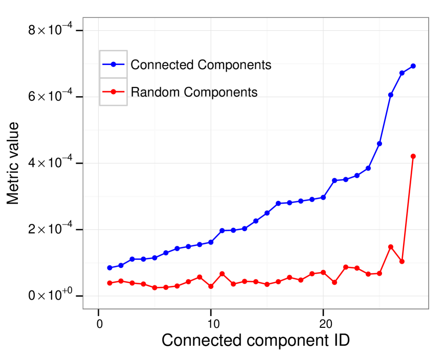
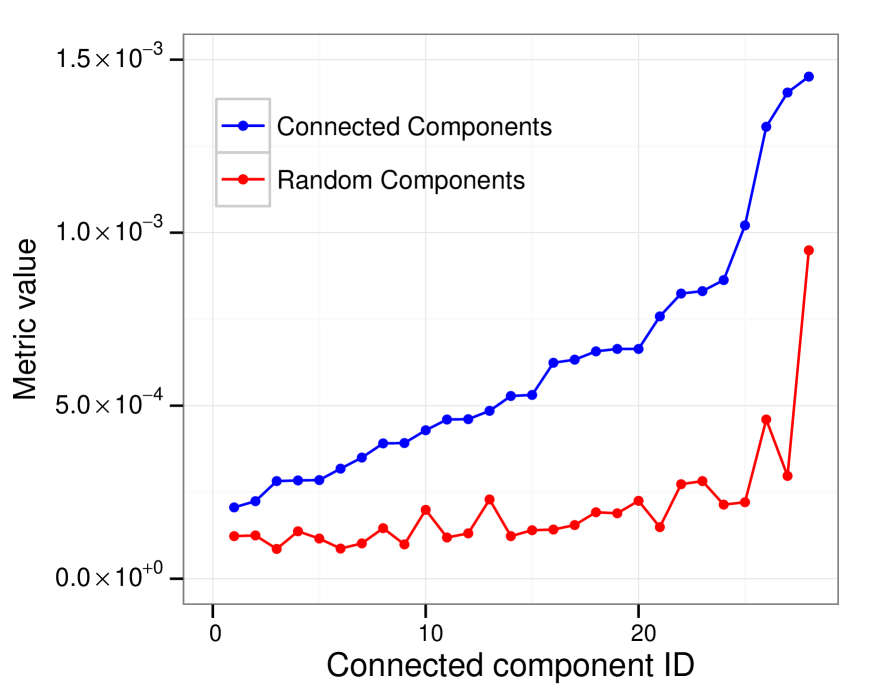
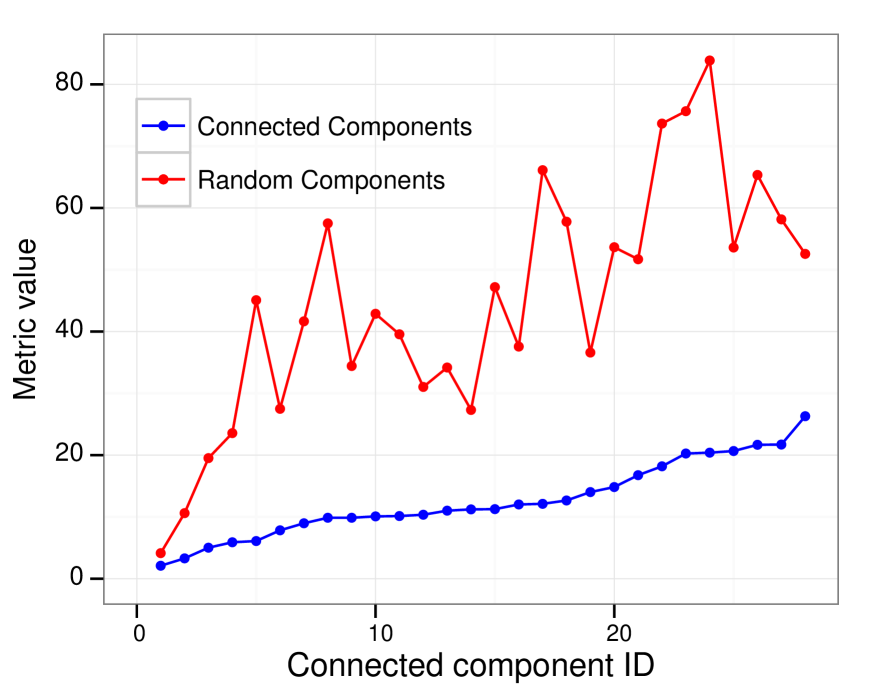
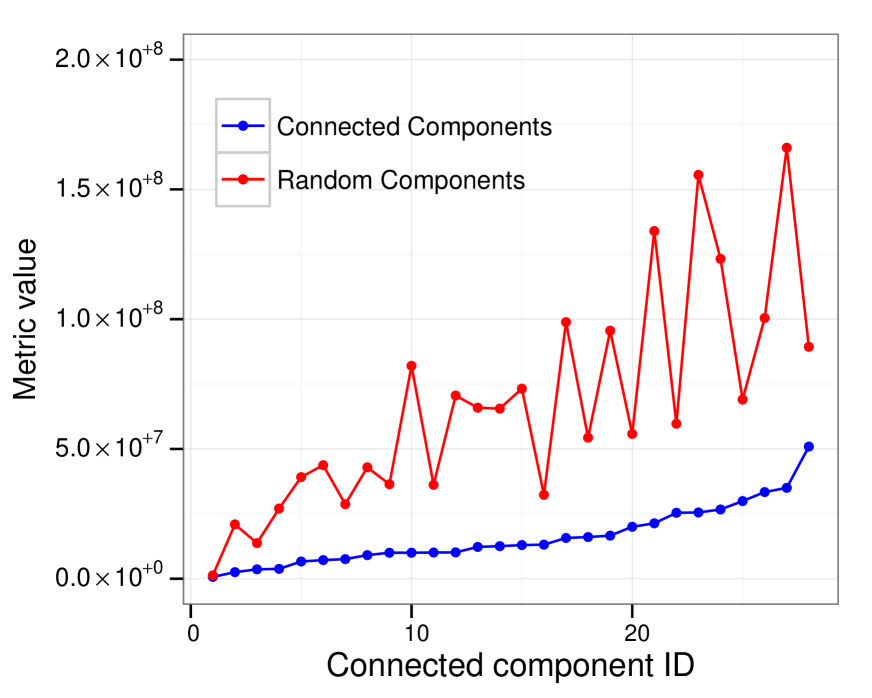
We performed experiments validating that merging keywords by forming connected components indeed produced meaningful groups of keywords representing an event. As a baseline, we used components obtained by merging random keyword pairs together. We evaluated how well a cluster is formed from the set of tweets obtained from connected components, comparing the cluster to the set of tweets obtained from random components. Connected components are expected to merge keyword pairs that belong to the same event, and hence would make better clusters when compared to merging random keyword pairs. The results are displayed in Figure 11. In this figure, each plot depicts a different metric that evaluates the quality of a cluster. These clustering metrics are summarized in Table 8. For better interpretation and visual clarity, in each of the plots, we sorted the clustering metrics obtained via connected components. We then rearranged the clustering metrics for the baseline according to the sorting order obtained from connected components. (This is the reason why the blue line is monotonically increasing.) This experiment was performed on one month of data (there are approximately 30 data points in each plot) between August 2013 and September 2013. We took all the keyword pairs obtained in a day and found the connected components as in Figure 10. For random components, we merged the keyword pairs randomly. We took precautions to make sure that the size of the connected components and random components per day were comparable. That is, if we had connected components of sizes 6, 6, and 5 formed from keyword pairs on particular day, we made sure that similarly sized random components were also formed from the keyword pairs of the same day. Also, to make sure that tweets from any one keyword pair do not dominate the tweet set, we sampled an equal number of tweets from each keyword pair, and the same sample of tweets is used to calculate the clustering metrics in both the connected components approach and the random components approach. The random baseline has been averaged over 3 different rounds of experimentation.

Figure 10: This figure illustrates how we merge keyword pairs which represent the same event into larger components.

(a) $I_{1}$

(b) $I_{2}$

(c) $H_{1}$

(d) $H_{2}$

(e) $G_{1}$

(f) $G^{\prime}_{1}$

Figure 11: Each plot in this figure compares the quality of the cluster of tweets obtained from connected components and random components. The actual metric is shown in Table 8. In $I_{1},I_{2},H_{1},H_{2}$ higher value is better. In $G_{1},G_{1}^{{}^{\prime}}$, lower value is better. For visual clarity, the values obtained from connected components were sorted in ascending order, hence the blue line is monotonically increasing. The values obtained were rearranged in the same order as well.

Name	Metric	Meaning
$I_{1}$	$\sum_{i=1}^{k}\frac{1}{n_{i}}\sum_{(u,v)\in S_{i}}\text{sim}(u,v)$	Higher value is better
$I_{2}$	$\sum_{i=1}^{k}\sqrt{\sum_{(u,v)\in S_{i}}(u,v)}$	Higher value is better
$E_{1}$	$\sum_{i=1}^{k}n_{i}\frac{\sum_{v\in S_{i},u\in S}\text{sim}(u,v)}{\sqrt{\sum_{(u,v)\in S_{i}}\text{sim}(u,v)}}$	Lower value is better
$G_{1}$	$\sum_{i=1}^{k}\frac{\sum_{v\in S_{i},u\in S}\text{sim}(u,v)}{\sum_{(v,u)\in S}\text{sim}(v,u)}$	Lower value is better
$G_{1}^{{}^{\prime}}$	$\sum_{i=1}^{k}n_{i}^{2}\frac{\sum_{v\in S_{i},u\in S}\text{sim}(v,u)}{\sum_{(u,v)\in S_{i}}\text{sim}(u,v)}$	Lower value is better
$H_{1}$	$\frac{I_{1}}{E_{1}}$	Higher value is better
$H_{2}$	$\frac{I_{2}}{E_{1}}$	Higher value is better

Table 8: This table lists the clustering metrics used in Figure 11.

2 VQ Event Model

We introduce a novel vectorial representation based on a vector quantization of the interarrival time distribution, which we call “VQ-event model”. The most representative interarrival times are learned from a large training corpus. Each of the learned interarrival times is called a codeword, and the entire set of the learned interarrival times, the codebook.

We represent an event $e$, belonging to a collection of events $\mathcal{E}$, as a tuple $(\mathcal{K}_{e},\mathcal{M}_{e})$, where $\mathcal{K}_{e}$ is a set of keywords and $\mathcal{M}_{e}$ is a set of social media messages. Both the keywords and the messages are related to a real-world occurrence. As explained in Section The keywords are extracted in order to succinctly describe the occurrence, and the messages are posts from users about the event.

To learn the most representative interarrival times we perform the following: for each $e\in\mathcal{E}$ with messages $\mathcal{M}_{e}=[m_{1}^{e},m_{2}^{e},\ldots m_{n}^{e}]$ and their corresponding time-stamps $[t_{1}^{e},t_{2}^{e},\ldots t_{n}^{e}]$ where $t_{i}\leq t_{i+i}\forall i\in[1,n]$, we compute all the interarrival times $d_{i}^{e}=t_{i}^{e}-t_{i-1}^{e}$ (the value of $t_{0}$ is considered equal to $t_{1}$ for initialization purposes). Then, the values of $d_{i}^{e}$ for all events in $\mathcal{E}$ are clustered to identify the most representative interarrival times.

Once the most representative interarrival times have been learned, the vector quantizations for each event is produced as follows: for each event, obtain all the interarrival times, and quantize each of the interarrival times to the closest codeword in the codebook. This process is summarized in Algorithm 3. Line 1 collects all of the interarrival times for all the events in $\mathcal{E}$ in f. Line 2 is a clustering algorithm which takes f and the number of clusters $k$ as inputs and returns the centroids of the clusters as the output in c. The centroids can be thought of as the most representative interarrival times for the event set $\mathcal{E}$. After that, the interarrival times of each event $e$ is vector quantized in terms of the centroids to obtain a $k$-dimensional real valued representation of the event (Line 4). In this representation, each entry is percentage of messages with that particular codeword as the interarrival time.

Algorithm 3 learn_representation()

0: Event set $\mathcal{E}$, and number of codewords $k$ in the codebook.

0: A representation in $\mathbb{R}^{k}$ of each event $e=(\mathcal{K}_{e},\mathcal{M}_{e})\in\mathcal{E}$.

1: $\textbf{f}\leftarrow\{d_{i}^{e}|m_{i}^{e}\in\mathcal{M}_{e},e\in\mathcal{E}\}$

2: c $\leftarrow$ cluster($\textbf{f},k$)

3: for $e\in\mathcal{E}$ do

4:    e $\leftarrow$ vq($d_{i}^{e},\textbf{c}$ )

5: end for

3 High Activity Vs Low Activity Events

Once the collection of events is converted into their VQ-event model representation, we can identify events that have produced similar levels of activity in the social network. In other words, events are considered to have similar activity if the interarrival times between their social media posts are similarly distributed, implying a very much alike collective reaction from users to the events within a group. In order to identify groups of similar events, we cluster the event models. We sort the resulting groups of events from highest to lowest activity, according to the concentration of social media posts in the bins that correspond to short interarrival times. We consider the events that fall in the top cluster to be high-activity events as most of their interarrival times are concentrated in the smallest interval of the VQ-event model. Thus we end with four groups of events: high, medium-high, medium-low and low. shows a heatmap of the interarrival relative frequency for each cluster.

Through this section, we analyze different features for each of the event categories and compare them both qualitatively and quantitatively. We peformed two-tailed $t$-tests for a variety of features for events in the high-activity category, and compare it with the average values for the remaining events.

3.1 Information Forwarding Characteristics

We found that the high-activity events possess more information forwarding characteristics than other events. We present four features which support this argument. The features, their description and their values are listed in Table 9.

The retweet_count is generally higher for high-activity events. This feature is the fraction of retweets present in the event, log-normalized by the total amount of tweets in the event. A higher value suggests that people have a greater tendency to spread the occurrence of these events, and forward this information to their followers.

The tweets_retweeted is lower for high-activity events than for the rest. This feature is the number of tweets which have been retweeted, log-normalized by the total number of tweets in the event. This suggests that the high amount of retweets for the high-activity events actually originates from fewer tweets. This suggests that fewer tweets become popular and are retweeted several times.

The retweets_most_retweeted is the total number of retweets of the tweet that has been retweeted the most. This number is much higher for high-activity events than for low-activity events, suggesting that the most popular tweet indeed becomes very popular when the event is of high-impact.

Feature Name	Description	high-activity, others	Hypothesis, $p$-value
retweet_count	20cm$\log($total retweet count
in the event divided by total
tweets in the event$)$	$2.205,1.473$	$1$, $p=0$
tweets_retweeted	20cm$\log($number of tweets
retweeted divided by
total tweets in the event$)$	$-1.091,-0.964$	$1$, $p=2.7\times 10^{-5}$
retweets_most_retweeted	20cmnumber of tweets of the most
retweeted tweet	$284.491,40.261$	$1$, $p=0$

Table 9: (Refer to Section 3.1.) This table lists all the features which characterize the information forwarding aspect of an event. In general, high-activity events tend to have higher values for information forwarding features than other events.

3.2 Conversational Characteristics

We found that high-activity events in general tend to generate more conversation between users than the events in other categories. We observe this behavior through several features. Refer to Table 10.

Feature Name	Description	high-activity, others	Hypothesis, $p$-value
replies	20cm$\log($total replies divided by total tweets$)$	$-1.4016,-1.6474$	$1$, $p=10^{-4}$
norm_replies	20cm$\log($number of replies divided by
total number of unique users$)$	$-1.5796,-1.9294$	$1$, $p=6.7\times 10^{-4}$
tweets_replied	20cm$\log($number of tweets which generated
replies divided by total tweets$)$	$-1.7784,-2.0668$	$1$, $p=0.001$
uniq_users_replied	20cm$\log($unique users who have written
a reply divided by total tweets$)$	$-1.7524,-2.0352$	$1$, $p=0.001$

Table 10: (Refer to Section 3.2.) This table lists all the features which characterize the conversational aspect of high-activity and remaining events. Using these features, we argue in Section 3.2 that high-activity events tend to invoke more conversation amongst users than their counterparts.

The features replies and norm_replies both count the number of replies, but have been normalized slightly differently. Both have a higher value for high-activity events suggesting that high-activity events in general tend to spark more conversation between the users. The tweets_replied feature counts the number of tweets which have generated replies (it has been log-normalized by the total number of tweets in the event). This is also higher for high-activity indicating that such events on average have more tweets which invoke a reply from people. The uniq_users_replied feature counts the number of unique users who have participated in an conversation. Again, this number is found to be higher for high-activity events than for others suggesting that more users tend to engage in a conversation about these events. All these features collectively suggest that high-activity events tend to have a conversational characteristic associated with them.

3.3 Topical Focus Characteristics

We find that high-activity events have a lot more focus in terms of the topical content than the remaining events. This possibly suggests that when a news item is sensational, people seldom deviate from the topic of the news to other things.

We used four features listed in Table 11 to study the topic focus characteristics of high-impact events.

Feature Name	Description	high-activity, others	Hypothesis, $p$-value
uniq_words	20cm$\log($total unique words
divided by total tweets$)$	$-0.1982,0.1651$	$1$, $p=0$
uniq_chars	20cm$\log($total unique characters
divided by total tweets$)$	$2.0009,2.0456$	$1$, $p=0$
uniq_hashtags	20cm$\log($number of unique hashtags
divided by total tweets$)$	$-1.1126,0.8761$	$1$, $p=0$
uniq_urls	20cm$\log($number of unique urls
divided by total tweets$)$	$-0.7194,-0.4951$	$1$, $p=0$

Table 11: (Refer to Section 3.3.) This table summarizes all the features that were used to study the topical focus characteristics of high-activity events.

The number of unique words (uniq_words) and characters (uniq_chars) for high-activity events is lower than the remaining events suggesting that the information content for high-activity events is more focused than for the remaining events (as they do not need a diverse vocabulary). Hashtags on Twitter are a sequence of characters that follow the # symbol. Conventionally, their purpose is to indicate the topic of the tweet. Again, this number (uniq_hashtags; log-normalized by the total number of tweets) is lower for the high-activity events than for the remaining events. The number of unique URLs (uniq_urls; which can be taken to interpret similar semantics as the hashtags) is also lower for high-activity events than for the rest.

3.4 Early prediction of high-activity events

The results from sections 3.1, 3.2 and 3.3 suggest that high-activity events differ considerably from other events in terms of how they are received by the users and in terms of the response they invoke from the network.

In the next phase, our goal is to supervised machine learning only the early tweets of an event to predict whether an event will generate high-activity or not. A list of all the features used for classification is shown in Table LABEL:tab:feats. The classification was carried using logistic regression provided by the Weka package. The data was split approximately into $60-20-20$ of training, test and validation sets and the results were averaged over 5 runs of experiments.

Table 13 illustrates the prediction results from the earliest 5% of the tweets tweets, and from using all the tweets. We the false positive rate using only the early tweets is almost as good as the false positive rate using all the tweets. The same observation holds for the metrics precision and ROC-area as well. However, we observe an $18\%$ increase in the recall (0.455 to 0.540). This suggests that some high-activity events perhaps do not start displaying their unique characteristics well enough in their early stages.

	Early 5% Tweets		All Tweets
	high-activity	others	high-activity	others
high-impact	$194$	$232$	$230$	$196$
non-high-impact	$43$	$4\,765$	$47$	$4\,761$

Table 12: Confusion matrix while predicting the top 8% of events as high-activity. The predictions were made using the early 5% of the tweets, and by using all the tweets from the event.

	Early 5% Tweets				All Tweets
	FP-Rate	Precision	Recall	ROC-area	FP-Rate	Precision	Recall	ROC-area
high-activity	0.009	0.819	0.455	0.900	0.01	0.830	0.540	0.945
others	0.545	0.954	0.991	0.900	0.460	0.960	0.990	0.945

Table 13: Classification results of detecting whether an event from the top 8% is high-impact or not while predicting from features extracted from the earliest 5% of the tweets and from all the tweets belonging to the event.

Table 14: List of features used for characterization and classification. The “Normalization Method” column corresponds to the method used to normalize the value of the first column using the value of the second column. For example, the total number of retweets was normalized dividing it by the total number of tweets, and then taking the logarithm. Zero values were replaced by $10^{-8}$.

Feature Name	Normalized By	Normalization Method
component_size	None
total_seconds	total_tweets	$\log(x)-\log(y)$
total_tweets	None
total_retweets	total_tweets	$\log(x)-\log(y)$
total_tweets_retweeted	total_tweets	$\log(x)-\log(y)$
retweets_most_retweeted	total_retweets	$\log(x)-\log(y)$
total_mentions	total_tweets	$\log(x)-\log(y)$
total_unique_mentions	total_mentions	$\log(x)-\log(y)$
total_tweets_with_mention	total_tweets	$\log(x)-\log(y)$
total_tweets_with_mostfrequent_mention	total_tweets_with_mention	$\log(x)-\log(y)$
total_hashtags	total_tweets	$\log(x)-\log(y)$
total_unique_hashtags	total_hashtags	$\log(x)-\log(y)$
total_tweets_with_hashtag	total_tweets	$\log(x)-\log(y)$
total_tweets_with_mostfrequent_hashtag	total_tweets_with_hashtag	$\log(x)-\log(y)$
total_urls	total_tweets	$\log(x)-\log(y)$
total_unique_urls	total_urls	$\log(x)-\log(y)$
total_tweets_with_url	total_tweets	$\log(x)-\log(y)$
total_tweets_with_mostfrequent_url	total_tweets_with_url	$\log(x)-\log(y)$
total_unique_verified_users	total_verified_users	$\log(x)-\log(y)$
total_verified_users	total_tweets	$\log(x)-\log(y)$
total_unique_users	total_tweets	$\log(x)-\log(y)$
total_replies	total_unique_users	$\log(x)-\log(y)$
total_tweets_first_replied	total_tweets	$\log(x)-\log(y)$
total_unique_users_replied	total_unique_users	$\log(x)-\log(y)$
total_tweets_replied	total_tweets	$\log(x)-\log(y)$
total_words	total_tweets	$\log(x)-\log(y)$
total_unique_words	total_words	$\log(x)-\log(y)$
total_characters	total_tweets	$\log(x)-\log(y)$
total_rt_count	total_tweets	$\log(x)-\log(y)$
total_fav_count	total_tweets	$\log(x)-\log(y)$
total_positive_sentiment	total_tweets	$x/y$
total_negative_sentiment	total_tweets	$x/y$

References and Notes

- 1. Mohamed Ahmed, Stella Spagna, Felipe Huici, and Saverio Niccolini. A peek into the future: Predicting the evolution of popularity in user generated content. In Proceedings of the Sixth ACM International Conference on Web Search and Data Mining, WSDM ’13, pages 607–616, New York, NY, USA, 2013. ACM.
- 2. Albert-Laszlo Barabasi. The origin of bursts and heavy tails in human dynamics. Nature, 435(7039):207–211, 2005.
- 3. Jonah Berger and Katherine L Milkman. What makes online content viral? Journal of Marketing Research, 49(2):192–205, 2012.
- 4. Carlos Castillo, Mohammed El-Haddad, Jürgen Pfeffer, and Matt Stempeck. Characterizing the life cycle of online news stories using social media reactions. In Proceedings of the 17th ACM Conference on Computer Supported Cooperative Work and Social Computing, CSCW ’14, pages 211–223, New York, NY, USA, 2014. ACM.
- 5. Júlio Cesar dos Reis, Fabrício Benevenuto, Pedro Olmo S. Vaz de Melo, Raquel O. Prates, Haewoon Kwak, and Jisun An. Breaking the news: First impressions matter on online news. CoRR, abs/1503.07921, 2015.
- 6. L. Fei-Fei and P. Perona. A bayesian hierarchical model for learning natural scene categories. In Computer Vision and Pattern Recognition, 2005. CVPR 2005. IEEE Computer Society Conference on, volume 2, pages 524–531 vol. 2, June 2005.
- 7. Liang Gao, Chaoming Song, Ziyou Gao, Albert-László Barabási, James P Bagrow, and Dashun Wang. Quantifying information flow during emergencies. arXiv preprint arXiv:1401.1274, 2014.
- 8. Julien Gaugaz, Patrick Siehndel, Gianluca Demartini, Tereza Iofciu, Mihai Georgescu, and Nicola Henze. Predicting the future impact of news events. In Advances in Information Retrieval, pages 50–62. Springer, 2012.
- 9. Marco Guerini, Carlo Strapparava, and Gözde Özbal. Exploring text virality in social networks. In ICWSM, 2011.
- 10. José Luis Iribarren and Esteban Moro. Branching dynamics of viral information spreading. Physical Review E, 84(4):046116, 2011.
- 11. Karen Spärck Jones. A statistical interpretation of term specificity and its application in retrieval. Journal of Documentation, 28:11–21, 1972.
- 12. Márton Karsai, Kimmo Kaski, Albert-László Barabási, and János Kertész. Universal features of correlated bursty behaviour. Scientific reports, 2, 2012.
- 13. Haewoon Kwak, Changhyun Lee, Hosung Park, and Sue Moon. What is twitter, a social network or a news media? In Proceedings of the 19th International Conference on World Wide Web, WWW ’10, pages 591–600, New York, NY, USA, 2010. ACM.
- 14. Kristina Lerman and Tad Hogg. Using a model of social dynamics to predict popularity of news. In Proceedings of the 19th International Conference on World Wide Web, WWW ’10, pages 621–630, New York, NY, USA, 2010. ACM.
- 15. Cheng-Te Li, Man-Kwan Shan, Shih-Hong Jheng, and Kuan-Ching Chou. Exploiting concept drift to predict popularity of social multimedia in microblogs. Inf. Sci., 339(C):310–331, April 2016.
- 16. Qian Liu, Mi Zhou, and Xin Zhao. Understanding news 2.0. Inf. Manage., 52(7):764–776, November 2015.
- 17. Adam J Mills. Virality in social media: the spin framework. Journal of public affairs, 12(2):162–169, 2012.
- 18. Henrique Pinto, Jussara M. Almeida, and Marcos A. Gonçalves. Using early view patterns to predict the popularity of youtube videos. In Proceedings of the Sixth ACM International Conference on Web Search and Data Mining, WSDM ’13, pages 365–374, New York, NY, USA, 2013. ACM.
- 19. Bongwon Suh, Lichan Hong, Peter Pirolli, and Ed H Chi. Want to be retweeted? large scale analytics on factors impacting retweet in twitter network. In Social computing (socialcom), 2010 ieee second international conference on, pages 177–184. IEEE, 2010.
- 20. Gabor Szabo and Bernardo A. Huberman. Predicting the popularity of online content. Commun. ACM, 53(8):80–88, August 2010.
- 21. Pang-Ning Tan, Michael Steinbach, and Vipin Kumar. Introduction to Data Mining, (First Edition). Addison-Wesley Longman Publishing Co., Inc., Boston, MA, USA, 2005.
- 22. Alexandru Tatar, Marcelo Dias de Amorim, Serge Fdida, and Panayotis Antoniadis. A survey on predicting the popularity of web content. Journal of Internet Services and Applications, 5(1):1–20, 2014.
- 23. Alexandru Tatar, Jérémie Leguay, Panayotis Antoniadis, Arnaud Limbourg, Marcelo Dias de Amorim, and Serge Fdida. Predicting the popularity of online articles based on user comments. In Proceedings of the International Conference on Web Intelligence, Mining and Semantics, WIMS ’11, pages 67:1–67:8, New York, NY, USA, 2011. ACM.
- 24. Telegraph. Chile news. http://www.telegraph.co.uk/news/worldnews/southamerica/chile/.
- 25. Twitter API. https://dev.twitter.com.
- 26. Twitter Inc. https://www.twitter.com.
- 27. Yonatan Vaizman, Brian McFee, and Gert Lanckriet. Codebook-based audio feature representation for music information retrieval. IEEE/ACM Trans. Audio, Speech and Lang. Proc., 22(10):1483–1493, October 2014.
- 28. Qiang Yan, Lianren Wu, Chao Liu, and Xiye Li. Information propagation in online social network based on human dynamics. In Abstract and Applied Analysis, volume 2013. Hindawi Publishing Corporation, 2013.