Signatures of double-electron re-combination in high-order harmonic generation driven by spatially inhomogeneous fields

Abstract

We present theoretical studies of high-order harmonic generation (HHG) driven by plasmonic fields in two-electron atomic systems. Comparing the two-active electron and single-active electron approximation models of the negative hydrogen ion atom, we provide strong evidence that a double non-sequential two-electron recombination appears to be the main responsible for the HHG cutoff extension. Our analysis is carried out by means of a reduced one-dimensional numerical integration of the two-electron time-dependent Schrödinger equation (TDSE), and on investigations of the classical electron trajectories resulting from the Newton’s equation of motion. Additional comparisons between the negative hydrogen ion and the helium atom suggest that the double recombination process depends distinctly on the atomic target. Our research paves the way to the understanding of strong field processes in multi-electronic systems driven by spatially inhomogeneous fields.

The incessant development of ultrafast, femtosecond ($10^{-15}$ fs) laser technology in the infrared (IR) regime opened new avenues to study a wide range of strong-field laser matter processes at their natural time scale Nisoli et al. (1997); L’Huillier and Balcou (1993); Krausz and Ivanov (2009). These invaluable experimental and technological tools allowed physicists to address instrumental aspects of one of the most fundamental processes: the tunneling ionization of atoms and molecules Krausz and Ivanov (2009). In particular, the application of this laser technology provided a key factor for the understanding of the main mechanisms underlying the emission of coherent radiation from atoms or molecules Ferray et al. (1988); L’Huillier and Balcou (1993); Corkum (1993); Lewenstein et al. (1994).

As a matter of fact, one could say the high-order harmonic generation (HHG) process fits within the tunneling ionization regime, when the Keldysh parameter, defined by $\gamma=\sqrt{\frac{I_{p}}{2U_{p}}}$, is $\gamma\leq 1$. $I_{p}$ and $U_{p}=\frac{\mathcal{E}_{0}^{2}}{4\omega_{0}^{2}}$ denote here the ionization potential of the atomic target, and the electron ponderomotive potential energy in atomic units, respectively. $\mathcal{E}_{0}$ is the peak amplitude of the laser electric field and $\omega_{0}$ the carrier frequency. The so-called three-step or “simple man’s” picture describes the underlying physics behind the HHG phenomenon Corkum (1993). In the first step, occurring about the maximum of the strong laser electric field, the Coulomb potential is deformed in such a way that a potential barrier is formed. Then, the electron is able to tunnel out throughout this “atomic barrier”, and the atom is then ionized. In the second step, or better to say phase, once the electron is in the continuum, the electric field of the laser accelerates it. Naturally, the electron gains energy from the oscillating field, converting it into a kinetic energy. Consequently, when the electric field changes its sign, the electron reverses the direction of its motion and has a certain probability to recombine back to the ground state of the remaining ion-core. In this third step it emits its energy excess as an attosecond burst of coherent radiation, typically in the XUV or EUV spectral range. In particular, the maximum emitted harmonic order is about $n=(I_{p}+3.17U_{p})/\omega_{0}$, and this result can be explained using purely classical arguments Corkum (1993); Lewenstein et al. (1994).

One of the main challenges in the production of HHG driven by IR femtosecond laser fields is the requirement of extra laser cavities for increasing up the peak power of the oscillator output, given the fact that intensities of the order of 10${}^{13}\sim 10^{14}$ W/cm² are needed for the HHG process to happen in atoms. A step forward to mitigate this issue was proposed by Kim and co-workers Kim et al. (2008a). By focusing a laser pulse of moderate intensity, 10¹¹ W/cm², coming directly from a femtosecond oscillator output, onto a bow-tie-shaped gold nano-structure array, an enhancement of about $20$ dB of the laser peak intensity on each of the elements was obtained. When Argon atomic gas was injected in the vicinity of each nano-structure, high-order harmonic emission of the fundamental frequency laser-beam was observed Kim et al. (2008a).

One should stress, however, that the experimental outcomes of Kim’s experiment are controversial (see e.g. Sivis et al. (2012); Kim et al. (2008b); Sivis et al. (2013)); nevertheless, they have stimulated incessant and promising theoretical activities. The pioneering theoretical works performed on HHG driven by plasmonic fields have confirmed two main facts, namely: (i) an enhancement of the emitted harmonics signal, and (ii) a large extension in the harmonic cutoff. These two features are mainly due to the spatial variation at a nanometer scale of the laser electric field along the laser polarization axis (see e.g. Husakou et al. (2011); Ciappina et al. (2012a); Yavuz et al. (2012); Ciappina et al. (2012b); Pérez-Hernández et al. (2013)).

Most of the approaches to model HHG, both driven by conventional and spatial inhomogeneous fields, are based on the hypothesis that a single active electron (SAE) approximation is good enough to describe the harmonic emission. Thereby, those pictures neglect electron-electron interactions in the atomic systems commonly used to produce high harmonics, such as He, Ar, Xe, etc. Ferray et al. (1988). Nevertheless, studies of HHG considering two- and multi-electron effects have been performed by several authors Lappas et al. (1996); Grobe and Eberly (1993a); Koval et al. (2007); Bandrauk and Lu (2005); Shi-Lin and Ting-Yun (2013); Santra and Gordon (2006); Prager et al. (2001). From these contributions one could conclude that depending on the atomic target properties and the laser frequency-intensity regime, multi-electron effects could play an important role in HHG Grobe and Eberly (1993a); Lappas et al. (1996); Koval et al. (2007). We should mention, however, that all these theoretical approaches have been developed for spatial homogeneous fields and that, to the best of our knowledge, studies of HHG in two-electron systems driven by spatially inhomogeneous fields have not been reported yet.

In this Letter we propose plasmonic fields as a tool to study multi-electron effects in HHG from two-electron systems. We focus our investigations on the study of the two-electron negative hydrogen ion (H^-) and the helium atom (He). By comparing the numerical solutions of the reduced 1D$\times$1D-TDSE for both the two-active electron (TAE), and the SAE models, we can trace out the analogies and differences in the HHG process from these two atomic systems, a priori very similar in their intrinsic structure. The interpretation of our numerical results renders on a semiclassical approach based on the time-frequency analysis of the quantum outcomes, and the classical integration of Newton’s equation of motion.

The 1D models of both H^- and He are described in Refs. Grobe and Eberly (1993a) and Lappas et al. (1996); Lein et al. (2000), respectively, and we shall thus present here only a brief summary. The HHG spectrum is computed by Fourier transforming the dipole acceleration $\langle a_{d}(t)\rangle$; for the TAE model it is thus mandatory to calculate the two-electron wave function $\Psi(z_{1},z_{2},t)$, while for the SAE model the one-electron wave function $\Psi(z,t)$ is sufficient. For this aim we numerically integrate the reduced 1D-TDSE for both models. In particular, in the case of the SAE approximation only the outer-electron is considered Lappas et al. (1996); Watson et al. (1997).

The Hamiltonian $H$ of our two-electron systems can be written in the length gauge as:

$$H=\frac{1}{2}\sum_{j=1}^{2}[p_{j}^{2}+V(z_{j})]+V_{ee}(z_{1},z_{2})+V_{\rm int}(t),$$ (1)

where $V(z_{j})=-\frac{Z}{\sqrt{z_{j}^{2}+a}}$ and $V_{ee}(z_{1},z_{2})=\frac{1}{\sqrt{(z_{1}-z_{2})^{2}+b}}$ are the $j$-th nucleus-electron soft-core Coulomb attractive potential, and the electron-electron soft-core Coulomb repulsion interaction for our two-electron system, respectively. Note that $V_{\rm int}(t)=\sum_{j=1}^{2}z_{j}(1+\frac{\epsilon}{2}z_{j})E_{\rm h}(t)$ defines the coupling of each of the two electrons with the plasmonic field in the dipole approximation for a linearly polarized laser field in the $z$-axis. The parameter $\epsilon$ denotes the inhomogeneity strength of the plasmonic field, and has units of inverse length (for more details see, e.g. Husakou et al. (2011); Ciappina et al. (2012a)). $E_{\rm h}(t)$, is a spatially homogeneous, or conventional laser electric field defined according to $E_{\rm h}(t)=\mathcal{E}_{0}f(t)\sin(\omega_{0}t+\varphi_{0})$, where $f(t)$ denotes the pulse envelope and $\varphi_{0}$ the carrier envelope phase (CEP).

For completeness we present also the one-electron Hamiltonian:

$$H=\frac{1}{2}p^{2}+V(z)+V_{\rm int}(t),$$ (2)

where a short-range Pöschl-Teller potential (PTP) $V(z)=-\frac{V_{0}}{2}\mu^{2}{\rm sech}^{2}(\mu z)$ Pöschl and Teller (1933); Chacón et al. (2015) is employed to model the outer-electron of our H^- system and now $V_{\rm int}(t)=z(1+\frac{\epsilon}{2}z)E_{\rm h}(t)$.

In order to compute the two-electron ground state of H^-, we set the soft-core parameters $a=b=1$ a.u., and the nuclear charge $Z=1$. Then, by imaginary time-propagation with a time step of $\delta t=-0.03i$ a.u., we integrate the laser-free Schrödinger equation and obtain the ground state wave function. This calculation yields a binding eigenenergy of ${E}_{0}=-0.73$ a.u. In our model for H^-, the $I_{p}$ of the inner-electron is $I_{p}^{(\rm i)}=0.66$ a.u., thereby the corresponding $I_{p}$ of the outer-electron will be about $I_{p}^{\rm(o)}\sim 0.1$ a.u. Grobe and Eberly (1993a, b)

For the SAE model, and in order to mimic the $I_{p}$ of the outer-electron $I_{p}^{\rm(o)}$ of the H^-, we chose for the PTP the screening parameter $\mu=1$, and $V_{0}=0.75$ a.u. The numerical solution of the 1D-TDSE for the TAE and SAE models is performed using the Split-Spectral Operator method (for more details see e.g. Feit et al. (1982); Frigo and Johnson ((1998); Ruiz and Chacón ((2008)).

Hence, to compute the HHG spectra, we first integrate numerically the 1D-TDSE for both models, and obtain the so-called dipole acceleration $\langle a_{d}(t)\rangle$ Grobe and Eberly (1993a); Lappas et al. (1996), which is the second order time derivative of electron position in the SAE model, and the sum of two such terms in the TAE case. The two-electron position grid space lengths are $L_{1}=L_{2}=2500$ a.u., with steps of $\delta z_{1}=\delta z_{2}=0.25$ a.u., respectively. The same grid parameters are used in case of the SAE approach, but only along a one-dimensional line. Afterwards, the emitted harmonic yield is computed by Fourier transforming the $\langle a_{d}(t)\rangle$, i.e. $I_{\rm HHG}=|\mathcal{FT}[\langle a_{d}(t)\rangle]|^{2}$. The emitted harmonic yields obtained within the TAE model were divided by a factor of 4, in order to take into account the two electrons of the atomic system. In this way a direct comparison with the SAE results can be made.

In addition to the quantum models, we have numerically solved the Newton’s equation $\dot{p}_{z}(t)=-[1+\epsilon z(t)]E_{\rm h}(t)$, to compute the classical highest electron energy at recollision $E_{\rm max}$. We note that the spatial inhomogenous electric field introduces substantial changes in the electron trajectory $z(t)$ (see e.g. Pérez-Hernández et al. (2013); Ciappina et al. (2012a)). For conventional fields, i.e. when $\epsilon=0$, this maximum energy at recollison is given by the usual expression $E_{\rm max}=3.17U_{p}$ Corkum (1993). The classical calculation of $E_{\rm max}$ allows us to estimate the maximum harmonic order $n_{1}=({I_{p}^{(\rm o)}+E_{\rm max}})/{\omega_{0}}$ of the HHG process driven by the inhomogeneous field. To distinguish between the conventional cutoff and the cutoff for the spatial inhomogeneous field, we shall denote them as $n_{1}$ and $n_{1}^{\prime}$, respectively.

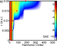
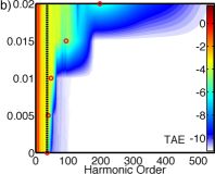
Figure 1: (color online) HHG yield of H^- driven by an inhomogeneous field in “logarithm scale” for (a) the SAE and (b) the TAE approximations, respectively. Black vertical dashed lines denote the cutoff for the SAE conventional field $n_{1}$ (a) and the TAE $n_{2}$ (b). Red circles are the calculated classical cutoffs as a function of $\epsilon$ according to our definition of $n_{1}^{\prime}$ and $n_{2}^{\prime}$ (see the text for more details). The IR laser pulse parameters are: peak intensity $I_{0}=2.0\times 10^{14}$ W$\cdot$cm^-2, $\omega_{0}=0.057$ a.u. (photon energy 1.55 eV), $\varphi_{0}=0$ rad., and $f(t)=\sin^{2}(\frac{\omega_{0}t}{2N})$ with 3 total cycles (the corresponding FWHM is 2.6 fs).

Fig. 1 shows the HHG spectra of the H^- as a function of the inhomogeneity degree, governed by $\epsilon$, for both the SAE (Fig. 1(a)) and TAE (Fig. 1(b)) models. Clearly, as $\epsilon$ increases, noticeable discrepancies in the harmonic emission structure and the cutoff are observed between the models. In case of SAE approach depicted in Fig. 1(a), the classical cutoff, $n_{1}^{\prime}$, is in very good agreement with the maximum energy of the emitted photon. On the contrary, for the TAE model, the classical predicted maximum harmonic order, $n_{1}^{\prime}$, is unable to match the cutoff obtained quantum mechanically, even for the case of $\epsilon=0$. Hence, we denote this “new” cutoff for the H^- TAE model by $n_{2}$. Logically, a natural question arises: where this clear disagreement between the SAE and TAE model comes from (note that the disparity is clearly visible for both conventional and spatial inhomogeneous electric fields cases).

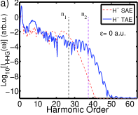
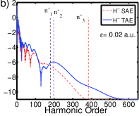
Figure 2: (color online) (a) conventional and (b) inhomogeneous emitted HHG spectra of H^- for our SAE and TAE models. In the HHG driven by a conventional field, the classical cutoff energy for the SAE and TAE calculations are denoted by $n_{1}$ (black vertical dashed line) and $n_{2}$ (violet vertical dashed line), respectively. The $n_{1}^{\prime}$, $n_{2}^{\prime}$ and $n_{3}^{\prime}$ (red vertical dashed line) denote the cutoff for the SAE, TAE and the double non-sequential two-electron re-combination mechanism (see the text), respectively.

In order to address the above question, in Figs. 2(a) and  2(b) we compare the emitted HHG spectra for two specific cases: the conventional case $\epsilon=0$ and an inhomogeneous case with $\epsilon=0.02$ a.u., respectively.

On the one hand, for conventional fields and in the case of two-electron systems, where double-electron ionization contributions are not relevant, one can expect that the cutoffs $n_{1}$ and $n_{2}$ coincide Lappas et al. (1996). The results depicted in Fig. 2(a) clearly shows this is not the case: an extra extension in the $I_{\rm HHG}^{\rm(TAE)}(\omega)$ cutoff with respect to the SAE model, is found. According to Lappas et al. Lappas et al. (1996) possible inner-electron contributions to the harmonic spectrum should extend the cutoff by an extra amount of $n_{\rm{shift}}=(I_{p}^{\rm(i)}-I_{p}^{\rm(o)})/\omega_{0}$ Lappas et al. (1996); Grobe and Eberly (1993a); Koval et al. (2007). Hence, we argue that the main mechanism behind this HHG extension is the sequential double-electron ionization of the outer- and inner-electrons, and re-collision of both of them Koval et al. (2007). This leads to a cutoff given by $n_{2}=n_{1}+n_{\rm shift}$ which is in reasonable agreement with the HHG spectrum computed by our TAE model.

On the other hand, Fig. 2(b) shows the emitted HHG spectra driven by a spatial inhomogeneous field for both the SAE and TAE models. Firstly, and similarly to the conventional field case, a structural difference between the models is observed in the HHG spectra, which comes from the different events of the electron re-combinations. Furthermore, the harmonic cutoff predicted by the SAE model is well reproduced by $n_{1}^{\prime}$. Secondly, a large high harmonic energy “cutoff” appears in the case of the computed HHG by means of the TAE model. That “cutoff” cannot be explained by $n_{2}^{\prime}$, even when the shift $n_{\rm shift}$ is included. This means that another mechanism is responsible for this extension. One candidate to explain this extension could be a double non-sequential two-electron re-combination event Koval et al. (2007). In order to probe this hypothesis, from classical calculations we can infer that the two electrons will re-combine to the ground state with maximum energies $E_{\rm max}^{\rm(1st)}$ and $E_{\rm max}^{\rm(2nd)}$, respectively, and then the emitted harmonic order cutoff could be obtained from Koval et al. (2007):

$$n_{3}^{\prime}=(E_{\rm max}^{\rm(1st)}+E_{\rm max}^{\rm(2nd)}+I_{p}^{\rm(i)}+I_{p}^{\rm(o)})/\omega_{0},$$ (3)

where, $E_{\rm max}^{\rm(1st)}$ and $E_{\rm max}^{\rm(2nd)}$ denote the maxima first (inner-electron) and second (outer-electron) re-collision energies, respectively. From Fig. 2(b) we observe that the predictions of Eq. (3) are in excellent agreement with our TAE model calculations (see the vertical dashed red line). Next, we shall explain in detail the underlying physics of Eq. (3).

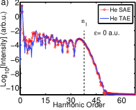
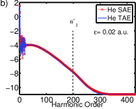
Figure 3: (color online) HHG for the He atom. The HHG spectra of (a) and (b) are computed with the same parameters as in Fig. 2. Black dashed vertical lines denote the $n_{1}$ conventional field cutoff for the outer-electron (a), and $n_{1}^{\prime}$ the inhomogeneous field cutoff (b).

Pursuing to find a broader panorama about the behavior of two-electron systems we have computed the HHG spectra of the He atom for both conventional and spatially inhomogeneous fields. The same SAE and TAE models of He described in Lappas et al. (1996); Lein et al. (2000) have been implemented. Similarly to the H^-, for the SAE approach we have integrated in a 1D-TDSE the outer-electron of He. In such a case the electron is simulated by the long-range soft-core Coulomb potential described in Lappas et al. (1996). The outer-electron $I_{p}$ of our He model is about $I_{p}^{\rm(o)}=0.73$ a.u. The results of the HHG spectra for both the conventional and spatial inhomogeneous fields are depicted in Figs. 3(a) and 3(b), respectively. Clearly, we can observe that both approaches are in perfect agreement for both cases. Slightly reasonable discrepancies are found for low-order harmonics, a region where the details of the atomic potential are relevant. In addition, both the SAE and TAE models’ cutoffs are identical, and as a consequence we argue that the outer-electron is the main responsible of HHG emission process in case of He. Note that an intensity scan of 1$\times$10¹⁴ – 9$\times$10¹⁴ W/cm² in the calculation of the HHG spectra have been performed for different values of $\epsilon$. Same degree of agreement between the SAE and TAE pictures was found. It is remarkable that neither an extra extension, $n_{\rm shift}$, nor an underestimation on the $n_{3}^{\prime}$ cutoff is observed for spatial inhomogeneous fields in the TAE model of He.

From this last asseveration, we can conclude that single- and double-electron ionization effects play an important role in the description of the emitted HHG from the H^- driven by both conventional and inhomogeneous fields. The latter provide a novel instrumental tool in order to enhance two-electron effects.

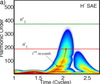
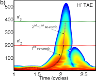
Figure 4: (color online) Gabor distributions and semiclassical analysis of the HHG driven by inhomogeneous fields for the SAE (a) and TAE (b) models of H^-. Violet circles depict the “classical” harmonic emission times considering the first electron re-combination events driven by the inhomogeneous field. In (b) the white triangles are the emitted harmonics by classically considering the first and the second double non-sequential two-electron re-combination events. In (a) the red and green horizontal dashed lines denote the cutoff $n_{1}^{\prime}$ and a modification of $n_{1}^{\prime}$ which takes into a count the first and second re-combination ($n_{1}^{\prime\prime}$) for the SAE. In case of the TAE model (b), the same horizontal lines depict the cutoffs denoted by $n_{2}^{\prime}$ and $n_{3}^{\prime}$ formulae (see the text).

In order to further clarify the reasons of the extended HHG spectra for the H^- we perform a time-analysis of the quantum mechanical results in terms of the Gabor distribution (for details see e.g. Gabor (1946); Chirila et al. (2010)). In short, information about the classical electron trajectories can be extracted from the HHG spectra computed via the TDSE, and compared with pure classical calculations.

Figure 4 depicts the Gabor distribution obtained from the quantum mechanically computed HHG spectra of the H^- system driven by an inhomogeneous field for both the SAE (Fig. 4(a)) and TAE (4(b)) models, respectively. The emitted harmonics calculated by the first and second classical re-collision electron-trajectories are also depicted. Excellent agreement between the Gabor synthesis and the classical calculations is found in case of the SAE picture. Note that only the first re-collisions are considered in the classical calculations shown in Fig. 4(a). However, when the TAE approach is employed, the first electron re-collision events are not sufficient to reproduce the whole range of emitted harmonics described by the Gabor time-frequency decomposition. Nevertheless, if one considers a second re-collision event in the classical approach, the maximum harmonic emission of Gabor’s distribution is then perfectly reproduced.

These observations suggest that the main mechanism behind the HHG spectra emitted from our two-electron H^- model driven by a spatially inhomogeneous field can be summarized as follows: (i) the outer-electron is ionized via tunneling about one of the maxima of the IR laser pulse. Then, after a while, around the second consecutive maxima, the inner-electron is liberated; (ii) as the single-electron and double-electron ionization probabilities are large, the outer-electron has a high chance to make a second re-collision event together with the first re-collision of inner-electron and both at the same re-combination time. This analysis indicates the emission of a “maximum” high-harmonic photon of order $n_{3}$ (see Eq. (3)). Then, the emitted photon at this particular time will be the sum of the first and second re-collision energies of the two electrons with their respective ground states. This picture is in perfect agreement with the Gabor distribution results, extracted from the quantum mechanical models. Furthermore, it is the spatially inhomogeneous character of the laser electric field which is the main responsible of the increase of the probability of this peculiar mechanism.

Additionally, the Gabor distribution of Fig. 4(a) helps us to disentangle if the inner- and outer-electron are re-combining with the remaining ion-core at the same re-collision time, or if it is only a first and second re-combination of a single-electron process. As it is clearly shown, there is not emitted harmonic signal at $n_{1}^{\prime\prime}=(E_{\rm max}^{\rm(1st)}+E_{\rm max}^{\rm(2nd)}+I_{p}^{(\rm o)})/\omega_{0}$. Then, it is not possible that the cutoff extension in the HHG spectra obtained from the TAE model comes from a single-electron ionization event followed by a first and second re-combinations event of this unique electron.

Hence, we believe we have collected convincing arguments, based both on quantum mechanical and classical analysis, that a new mechanism, a double non-sequential two-electron re-combination is the main responsible of the extension of the HHG spectra of the H^- when a spatial inhomogeneous plasmonic field is used to drive the process.

Summarizing, we performed two-electron calculations of HHG driven by spatial homogeneous and inhomogeneous fields. We used as test systems H^- and He. By the numerical solution of 1D-TDSE models in the two- and single-active-electron approximations, supported by a classical analysis of the electron trajectories, we demonstrated that an extra extension in the harmonic cutoff was found in case of the TAE model for H^-, which cannot be explained within the SAE framework. After a comprehensive analysis using complementary tools, we concluded that a new mechanism is the main responsible of this extension. One of the main advantages to use plasmonic fields as “probes” is the low incoming intensity needed in order to observe this effect, considering that the plasmonic nano-structures act as light amplifiers. In addition, as we have shown, the results strongly depend on the atomic system employed. In particular, the H^- was chosen for simplicity, but we consider similar effects and results could be found for highly correlated negative ion systems, such as the Alkali negative ions Clementi and McLean (1964).