Direct optical state preparation of the dark exciton in a quantum dot

Abstract

Because of their weak coupling to the electromagnetic field dark excitons in semiconductor quantum dots possess extremely long lifetimes, which makes them attractive candidates for quantum information processing. On the other hand, preparation and manipulation of dark states is challenging, because commonly used optical excitation mechanisms are not applicable. We propose a new, efficient mechanism for the deterministic preparation of the dark exciton exploiting the application of a tilted magnetic field and the optical excitation with a chirped, i.e., frequency modulated, laser pulse.

The optical properties of an exciton in a semiconductor quantum dot (QD) are determined by the combination of spin states of electron and hole. In the most common case of heavy hole excitons among the four different states the two excitons with antiparallel electron and hole spin are optically active or bright. The other two excitons with parallel spin do not couple to the light field and are called dark. The bright states have been proposed for various applications, e.g., as single photon sources Yuan et al. (2002); Santori et al. (2001); Press et al. (2007) or qubits Bonadeo et al. (1998); Biolatti et al. (2000); Troiani et al. (2000); D’Amico et al. (2002); Boyle et al. (2008); Michaelis De Vasconcellos et al. (2010), and a large amount of research has been dedicated to their optical state preparation and control Ramsay (2010); Reiter et al. (2014). Dark excitons seem to be optically inaccessible and have almost no influence on bright excitons; therefore they are often neglected. But dark excitons offer unexplored potential for applications as photon memory or for quantum operations Korkusinski and Hawrylak (2013); Poem et al. (2010), because their lifetime exceeds the one of bright excitons by far Poem et al. (2010); McFarlane et al. (2009). For this reason it is very attractive to use dark excitons for quantum information applications and to overcome the huge challenge to prepare dark excitons in a controlled and direct manner.

In this Communication we propose a method to optically prepare dark excitons in a deterministic way. Other methods to optically access dark excitons have been proposed recently, either relying on the relaxation from higher excited and biexciton states Poem et al. (2010); Korkusinski and Hawrylak (2013); Smoleński et al. (2015); Schmidgall et al. (2015) or on valence band mixing caused by asymmetry Schwartz et al. (2015). In contrast, in our proposal dark excitons are directly excited from the QD ground state and the excitation mechanism can be applied to all typical II-VI and III-V QDs. Our preparation scheme uses two simple ingredients: a chirped laser pulse and a tilted magnetic field. Chirped laser pulses have already shown great potential for preparation of bright excitons and biexcitons via adiabatic rapid passage (ARP) Wu et al. (2011); Simon et al. (2011); Mathew et al. (2014); Lüker et al. (2012); Gawarecki et al. (2012); Glässl et al. (2013); Debnath et al. (2012); Malinovsky et al. (2013). The in-plane component of a magnetic field couples bright and dark exciton via a spin-flip Bayer et al. (2000); Besombes et al. (2000); Kazimierczuk et al. (2011) and therefore transfers oscillator strength to the dark exciton. We will show how the clever combination of these two ingredients allows for an efficient dark exciton preparation.

We consider a self-assembled QD, where the uppermost valence band is of heavy-hole type, i.e., the holes have a spin of $S^{h}_{z}=\pm 3/2$ while the electrons have a spin of $S^{e}_{z}=\pm 1/2$. This leads to the formation of four single exciton states with total spin $J_{z}=S^{h}_{z}+S^{e}_{z}\in\{\pm 1,\pm 2\}$. According to the dipole selection rules only excitons with a total spin of $+1$ ($-1$) can be optically excited, which corresponds to excitation with positive (negative) circularly polarized laser pulses. We label the corresponding bright states $|b^{+}\rangle$ ($|b^{-}\rangle$). Excitons with total spin of $+2$ ($-2$) are not optically active and labeled $|d^{+}\rangle$ ($|d^{-}\rangle$). The biexciton state is denoted by $|B\rangle$. The short range exchange interaction gives rise to a splitting $\delta_{0}$ between bright and dark excitons. In most real QDs the bright excitons $|b^{\pm}\rangle$ are coupled by the long range exchange interaction leading to linearly polarized excitons with a splitting $\delta_{1}$. Analogously, the dark excitons $|d^{\pm}\rangle$ are coupled and split by $\delta_{2}$.

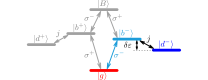
Figure 1: (Color online) Schematic level diagram.

An external magnetic field $\mathbf{B}$ is used to control the level structure of the system and the coupling between the states. The out-of-plane component of the magnetic field $B_{z}$ provides a control parameter for the exciton energies via the Zeeman shifts of the electron (hole) determined by the out-of-plane $g$-factors $g_{e,z}$ ($g_{h,z}$) Bayer et al. (1999). The in-plane magnetic field $B_{x}$ induces spin flips of the electron (hole) via the in-plane $g$-factors $g_{e,x}$ ($g_{h,x}$). While the model is applicable to many materials, here, we take GaAs material parameters Bayer et al. (2000, 2002); Kuther et al. (1998). The Hamiltonian together with the material parameters is given in the supplemental information.

The choice of the magnetic field and in particular the ratio between out-of-plane and in-plane component of the magnetic field is crucial in our set-up. On the one hand the in-plane magnetic field is needed to couple bright and dark exciton to enable dark exciton state preparation, on the other hand it should be weak such that bright and dark exciton are still well-defined. We find that these conditions are fulfilled for $B_{z}=4\,{\rm{T}}$ and $B_{x}=3\,{\rm{T}}$. The level structure of the six states for these parameters is depicted in Fig 1.

It turns out that for the chosen magnetic field, when restricting ourselves to the case of excitation with $\sigma^{-}$-polarized light, the system can be reduced to a three-level model consisting of the states $|g\rangle$, $|b^{-}\rangle$, and $|d^{-}\rangle$ (colored states in Fig. 1). Therefore, in the following discussions we will concentrate on this reduced model and omit the polarization superscript “$-$” of the exciton states. The three-level model is characterized by the energy difference $\delta\epsilon=\delta_{0}-g_{e,z}\mu_{B}B_{z}=0.43\,{\rm{meV}}$ and the coupling $j=\frac{1}{2}\mu_{B}g_{e,x}B_{x}=0.056\,{\rm{meV}}$. With these values, the admixture of the bright exciton to the dark exciton is only about 1.5 %. Thus the lifetime of the dark exciton is expected to be still about two orders of magnitude larger than the lifetime of the bright exciton Stevenson et al. (2004).

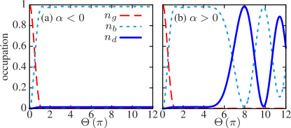
Figure 2: (Color online) Final occupation of ground state $n_{g}$ (red dashed line), bright exciton $n_{b}$ (light blue dotted line), and dark exciton $n_{d}$ (solid blue line) after excitation with a pulse with pulse area $\Theta$ and for (a) negative chirp $\alpha=-40\,{\rm{ps}^{2}}$, and (b) positive chirp $\alpha=+40\,{\rm{ps}^{2}}$.

We consider an excitation with a chirped laser pulse, which has been shown to yield a population inversion of the bright exciton system, being stable against small changes of the pulse parameters Wu et al. (2011); Simon et al. (2011); Reiter et al. (2014); Debnath et al. (2012). The instantaneous frequency of the pulse $\omega(t)=\omega_{0}+at$ changes with the chirp rate $a$, while its envelope is characterized by the pulse area $\Theta$ and the duration $\tau$. Such a linearly chirped Gaussian pulse can be obtained by sending a transform-limited Gaussian laser pulse with duration $\tau_{0}$ through a chirp filter with chirp coefficient $\alpha$. For our calculations we use pulses with an initial duration $\tau_{0}=3.5\,{\rm{ps}}$ and a chirp coefficient $\alpha=\pm 40\,{\rm{ps}}^{2}$, which yields chirped pulses with $\tau\approx 12\,{\rm{ps}}$ and $a\approx\pm 0.023\,{\rm{ps}}^{-2}$ (for details see supplemental information). The central frequency $\omega_{0}$ at the pulse maximum is taken to be in resonance with the bright exciton transition.

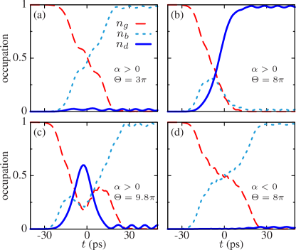
Figure 3: (Color online) Temporal evolution of the occupation of ground state $n_{g}$ (red dashed line), bright exciton $n_{b}$ (light blue dotted line), and dark exciton $n_{d}$ (solid blue line) for $\alpha=40\,{\rm{ps}}^{2}$ and (a) $\Theta=3\pi$, (b) $\Theta=8\pi$, and (c) $\Theta=9.8\pi$. (d) Same as part (b), but for negative chirp $\alpha=-40\,{\rm{ps}}^{2}$.

For state preparation the common quantity to describe the excitation fidelity is the final occupation after the pulse Ramsay (2010); Reiter et al. (2014). Typically the final occupations are shown as a function of the laser pulse power expressed in terms of the pulse area $\Theta$. Figure 2(a) shows the final occupation of the ground state $n_{g}$, the bright exciton $n_{b}$, and the dark exciton $n_{d}$ as a function of pulse area for a negatively chirped pulse with $\alpha=-40\,{\rm{ps}}^{2}$. We find that the behavior is equivalent to ARP in a two-level system. As soon as the pulse area exceeds the adiabatic threshold a robust occupation of the bright exciton is seen. The dark exciton is completely unaffected and its occupation remains at $n_{d}=0$.

The situation changes dramatically when the sign of the chirp is reversed, i.e., for excitation with a positively chirped pulse, as depicted in Fig 2(b). While for pulse areas up to $\Theta\approx 5\pi$ the behavior is similar to the two-level case, for higher pulse areas the dark exciton becomes significantly occupied. At $\Theta=8\pi$ a maximal occupation of approximately $n_{d}=1$ is achieved. This is a remarkable result, since the dark exciton is not directly affected by the chirped laser pulse, but only coupled indirectly via the bright exciton to the light field. When the pulse area is increased further, we find that the final occupation oscillates between bright and dark exciton. To validate the approximation of the three-level system, we performed calculations in the full six-level system which showed that the sum of the occupations of the neglected states remains indeed well below 1%.

To understand the dynamics during the excitation in Fig. 3 we have plotted the temporal evolution of the state occupations for different excitation conditions. Figure 3(a) shows the case of a positively chirped laser pulse ($\alpha=40\,{\rm{ps}}^{2}$) and a pulse area of $\Theta=3\pi$. During the excitation the occupation of the bright exciton increases monotonically to $n_{b}=1$, while the ground state occupation goes to zero. The dark exciton is nearly unaffected. Hence the complete system can be considered as an effective two-level system consisting of ground state and bright exciton. After the pulse there are small oscillations between bright and dark exciton caused by the in-plane magnetic field. In agreement with our choice of magnetic field, these oscillations are so small that the discrimination between bright and dark exciton is still valid. To account for these oscillations all final occupations shown in this Communication are averaged over one period.

Figure 3(b) shows the dynamics at $\Theta=8\pi$, where the first maximum of the dark exciton occupation occurs. Initially the ground state occupation decreases, while the occupation of the bright exciton increases. Then, also the dark exciton becomes increasingly populated. The bright exciton occupation reaches a maximum around $t=-10\,{\rm{ps}}$ and subsequently drops to $n_{b}\approx 0$, just as the ground state occupation. The occupation of the dark exciton increases monotonically up to $n_{d}\approx 1$. The dynamics at $\Theta=9.8\pi$, i.e., at the first minimum of the final dark exciton occupation, is depicted in Fig. 3(c). First the population of the ground state drops down in favor of the bright and dark exciton occupation, until all three states are almost equally populated. During the peak intensity of the laser pulse all three occupations oscillate, the dark exciton occupation oscillating opposite to the ground state and bright exciton occupations. After one oscillation the dark exciton occupation returns to $n_{d}\approx 0$, while the bright exciton becomes almost completely populated. To complete the discussion of the dynamics, Fig. 3(d) shows the occupations for negative chirp $\alpha=-40\,{\rm{ps}}^{2}$ and $\Theta=8\pi$. We find that a population inversion between ground state and bright exciton takes place, but even for such high pulse areas the dark exciton occupation remains at $n_{d}\approx 0$. This confirms that the system can be reduced to a two-level system for excitation with negatively chirped laser pulses.

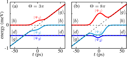
Figure 4: (Color online) Instantaneous eigenenergies corresponding to the dressed states $|\Psi_{1}\rangle$, $|\Psi_{2}\rangle$, and $|\Psi_{3}\rangle$, for (a) $\Theta=3\pi$ and (b) $\Theta=8\pi$. Dashed lines illustrate the evolution of the states without interaction.

A well established picture to understand the dynamics of a system under strong excitation is the dressed state picture Tannor (2007). Dressed states are the instantaneous eigenstates of the system, which are obtained by a diagonalization of the Hamiltonian, including light-matter interaction and magnetic field coupling. In general, each dressed state is composed of a mixture of all bare states $|g\rangle$, $|b\rangle$, and $|d\rangle$. Only for vanishing interaction a dressed state is identical to a bare state. In our system this happens in the limit of times long before and after the pulse because then also the coupling by $B_{x}$ can be neglected since $\delta\epsilon\gg j$.

Figure 4 shows the evolution of the instantaneous eigenenergies corresponding to the indicated dressed states in a frame rotating with the laser frequency. In Fig. 4(a) the pulse area is $\Theta=3\pi$, which is in the parameter region where we found a behavior like in a two-level system. The system is initially in the ground state $|g\rangle$, which agrees with the dressed state $|\Psi_{3}\rangle$ for times long before the pulse. The system evolves adiabatically along the branch which is related to $|\Psi_{3}\rangle$ in Fig. 4(a). Around $t=-30\,{\rm{ps}}$ this branch crosses the dressed state $|\Psi_{2}\rangle$, which corresponds to the dark exciton. The system evolves straight through this crossing, because the laser pulse is not yet effective and there is no direct coupling between ground state and dark exciton. Due to the chirp the system traverses afterwards a broad anti-crossing with the state $|\Psi_{1}\rangle$. This state agrees with the bright exciton for times long before the pulse. Because of the chirp the character of the dressed states changes during the pulse. For times long after the pulse the state $|\Psi_{3}\rangle$ can be identified as the bright exciton $|b\rangle$, which gives rise to the ARP effect Tannor (2007).

Let us now consider the evolution of the eigenstates at $\Theta=8\pi$, where the dark exciton becomes populated. Analogous to the case of low pulse area the system starts on the lowest branch $|\Psi_{3}\rangle$ and passes the crossing with $|\Psi_{2}\rangle$. The main difference is the size of the splitting between $|\Psi_{1}\rangle$ and $|\Psi_{3}\rangle$ around $t=0$, which is now much larger because of the high pulse intensity. This results in a strong bending of $|\Psi_{3}\rangle$ such that it approaches $|\Psi_{2}\rangle$. Because $|\Psi_{3}\rangle$ and $|\Psi_{2}\rangle$ are coupled, in accordance to the coupling between bright and dark state induced by the in-plane magnetic field, two additional anti-crossings between the two branches emerge. However, the splitting of these anti-crossings is small, such that the system cannot evolve adiabatically through them anymore. Instead, transitions between the involved branches occur resulting in quantum beats between the two dressed states. This is confirmed by our finding in Fig. 3(c), where the occupations of the states oscillate in time and also by the oscillatory behavior shown in the final occupation in Fig. 2(b). The final state of the oscillation is determined by the laser pulse intensity, i.e., the mixing of the states, and the duration of the quantum beats. Accordingly, after the second anti-crossing the system can end up either in $|\Psi_{2}\rangle$ or $|\Psi_{3}\rangle$, or any superposition between them. A similar picture is given by the optical Stark effect, by which for strong pulses bright and dark exciton can be brought into resonance such that quantum beats occur Reiter et al. (2012, 2013).

We again complete the discussion considering negative chirps. The change of the sign of the chirp is equivalent to a time reversal. This means that the dressed state diagrams have to be read backwards. When the QD is initially in the ground state the system now evolves along the upper branch $|\Psi_{1}\rangle$. Because $|\Psi_{1}\rangle$ is the uppermost dressed state and this state is always well separated from the other states, no transitions to $|\Psi_{2}\rangle$ are possible, i.e., a population of the dark exciton cannot be achieved and the system evolves adiabatically into the bright exciton state. However, if the QD has been driven into the dark exciton state by a pulse with positive chirp, the evolution caused by this pulse is reversed and the system evolves back into the ground state. Thus by applying a sequence of pulses with alternately positive and negative chirp the QD can be switched back and forth between ground state and dark exciton.

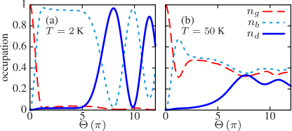
Figure 5: (Color online) Same as Fig. 2(b) including electron-phonon interaction at (a) $T=2\,$K and (b) $T=50\,$K.

A realistic QD is not completely isolated but interacts with its environment. Previous studies have shown that the coupling to phonon modes of the surrounding material is the main source of decoherence in QDs Ramsay (2010); Reiter et al. (2014). In the following we consider the coupling to longitudinal acoustic (LA) phonons via the deformation potential using GaAs material parameters within a well-established fourth-order correlation expansion (cf. supplemental information) Krügel et al. (2005); Lüker et al. (2012). Figure 5 shows the influence of the phonons on the final occupation of the three states for excitation with positively chirped laser pulses at two different temperatures $T=2$ K and $T=50$ K.

Previous calculations in the two-level system have shown that the effect of phonons on state preparation using ARP can be described by transitions between the dressed states Lüker et al. (2012); Gawarecki et al. (2012). For low temperatures, only phonon emission takes place, while phonon absorption processes are suppressed. Therefore, we do not expect a significant influence of the phonons, when positively chirped pulses are used for the dark exciton preparation, because the evolution takes place on the lowest branch of the dressed states. Even when the system is on the central branch after the anti-crossing no phonon-assisted transitions occur to the lower branch $|\Psi_{2}\rangle$, because the phonon coupling strength is the same for both bright and dark exciton. Indeed, as seen in Fig. 5(a), the influence of phonons is almost negligible for $T=2$ K and the behavior is similar to the phonon free case shown in Fig. 2(b). For higher temperatures, phonon absorption processes become possible, which results in an almost equal occupation of the three states as shown in Fig. 5(b), which is similar to the behavior of ARP in a two-level system Lüker et al. (2012).

In conclusion, we have shown that the excitation with a chirped laser pulse in combination with an external magnetic field provides a powerful tool for the optical preparation of dark excitons in QDs. The direct and deterministic preparation of the dark exciton is a crucial step towards the usage of dark excitons for applications, e.g., in quantum information processing.