A LOFAR census of non-recycled pulsars: average profiles, dispersion measures, flux densities, and spectra

We present first results from a LOFAR census of non-recycled pulsars. The census includes almost all such pulsars known (194 sources) at declinations ${\rm Dec}>8\degree$ and Galactic latitudes $|{\rm Gb}|>3\degree$, regardless of their expected flux densities and scattering times. Each pulsar was observed for $\geq 20$ minutes in the contiguous frequency range of 110–188 MHz. Full-Stokes data were recorded. We present the dispersion measures, flux densities, and calibrated total intensity profiles for the 158 pulsars detected in the sample. The median uncertainty in census dispersion measures ($1.5\times 10^{-3}$ pc cm^-3) is ten times smaller, on average, than in the ATNF pulsar catalogue. We combined census flux densities with those in the literature and fitted the resulting broadband spectra with single or broken power-law functions. For 48 census pulsars such fits are being published for the first time. Typically, the choice between single and broken power-laws, as well as the location of the spectral break, were highly influenced by the spectral coverage of the available flux density measurements. In particular, the inclusion of measurements below 100 MHz appears essential for investigating the low-frequency turnover in the spectra for most of the census pulsars. For several pulsars, we compared the spectral indices from different works and found the typical spread of values to be within 0.5–1.5, suggesting a prevailing underestimation of spectral index errors in the literature. The census observations yielded some unexpected individual source results, as we describe in the paper. Lastly, we will provide this unique sample of wide-band, low-frequency pulse profiles via the European Pulsar Network Database.

1 Introduction

Table 1: Criteria used to select the sources for the LOFAR census of non-recycled pulsars.

Parameter	Criteria	Reasoning
Declination (Dec)	$\mathrm{Dec}>8\degree$	Maximise the telescope sensitivity (which degrades with zenith angle, ZA, as $\sim\cos^{2}\mathrm{ZA}$).
Galactic latitude ($\mathrm{Gb}$)	$|\mathrm{Gb}|>3\degree$	Avoid higher sky background temperatures in the Galactic plane.
Surface magnetic field ($B_{\mathrm{surf}}$)	$B_{\mathrm{surf}}>10^{10}$ G	LOFAR observations of recycled pulsars were part of a separate project (Kondratiev et al., 2016).
Position error ($\epsilon_{\mathrm{RA}}$, $\epsilon_{\mathrm{Dec}}$)	$\epsilon_{\mathrm{RA}}<130\arcsec$ or $\epsilon_{\mathrm{Dec}}<130\arcsec$	In order to avoid non-detections or biased flux density measurements due to mispointings, the source position error was required to be less than the full-width at half-maximum of LOFAR’s HBA full-core tied-array beam, pointed towards zenith, at the shortest wavelength observed ($130\arcsec$, van Haarlem et al., 2013).
Association	field pulsar	Excluding globular cluster pulsars aimed at simplifying time budget calculation (“one pulsar per pointing”) for the initial version of census proposal and persisted by accident. Thus, four otherwise suitable pulsars in M15 and M53 are missing from the census sample.

Since their discovery almost 50 years ago (Hewish et al., 1968), the pulsations from pulsars – rapidly rotating, highly magnetised neutron stars – have been successfully detected over the entire electromagnetic spectrum, from the low radio frequencies at the edge of the ionospheric transparency window (10 MHz, Hassall et al., 2012) up to the very high-energy photons (1.5 TeV, MAGIC Collaboration et al., 2016). It is currently accepted that radiation processes at the various wavelengths of the electromagnetic spectrum are governed by several distinct emission mechanisms, with emission coming from different regions within the pulsar magnetosphere or from the star’s surface (Lyne & Graham-Smith, 2012).

The radio component of pulsar spectra is undoubtedly generated by coherent processes in the relativistic plasma of the pulsar magnetosphere (Lyne & Graham-Smith, 2012), but, despite decades of study, the exact mechanisms of the pulsar radio emission still remain unclear. Solving this problem would not only contribute to our knowledge of plasma physics under these extreme conditions, but also improve the understanding of pulsars as astrophysical objects and as probes of the interstellar medium (ISM).

The lowest radio frequencies (below 200 MHz) can provide valuable information for tackling this problem, because at these very low frequencies pulsar emission undergoes several interesting transformations, e.g. spectral turnover (Sieber, 1973) or rapid profile evolution (Phillips & Wolszczan, 1992). However, observing below 200 MHz is challenging because the diffuse Galactic radio continuum emission, with its strong frequency dependence (e.g. Lawson et al., 1987), significantly contributes to the system temperature at these lower frequencies. At the same time, the deleterious effects of propagation in the ISM become ever more powerful (Stappers et al., 2011), sometimes making it difficult to disentangle intrinsic pulsar signal properties from effects imparted by the ISM. Nevertheless, various properties of low-frequency pulsar radio emission have been previously investigated with the help of a number of telescopes around the globe.

The last decade was marked by rapid development of both hardware and computing capabilities, which made wide-band pulsar observing at low frequencies possible. A major receiver upgrade has been done on UTR-2 (Ryabov et al., 2010) and there are three new telescopes operating below 200 MHz: LOFAR (LOw-Frequency ARray, the Netherlands; van Haarlem et al., 2013), MWA (Murchinson Widefield Array, Australia; Tingay et al., 2013) and LWA (Long Wavelength Array, USA; Taylor et al., 2012).

LOFAR has already been used for exploring low-frequency pulsar emission, e.g. wide-band average profiles (Pilia et al., 2016), polarisation properties (Noutsos et al., 2015), average profiles and flux densities of millisecond pulsars (Kondratiev et al., 2016), drifting subpulses from PSR B0809+74 (Hassall et al., 2013), nulling and mode switching in PSR B0823+26 (Sobey et al., 2015), as well as mode switching in PSR B0943+10 (Hermsen et al., 2013; Bilous et al., 2014).

The first LOFAR pulsar census of non-recycled pulsars is a logical extension of these studies. Within the census project, we have performed single-epoch observations of a large sample of sources in certain regions of the sky, without any preliminary selections based on estimated peak flux density of the average profile or expected scattering time. Census observations resulted in full-Stokes datasets spanning the frequency ranges of LOFAR’s high-band antennas (HBA, 110–188 MHz) and, for a subset of pulsars, the low-band antennas (LBA, 30–90 MHz). The information recorded can be used for investigating the emission properties of about 150 pulsars, with the possibility of both average and single-pulse analyses. Based on census data, the properties of the ISM can also be explored using dispersion measures (DMs), scattering times, and rotation measures (RMs).

This paper presents the first results of the high-band part of the census project (analysis of the LBA data is deferred to subsequent work). Sect. 2 describes the sample selection, observing setup and the initial data processing for the HBA data. In Sect. 3 we discuss the source detectability versus scattering time and DM, and discuss the DM variation rates obtained by comparing census DMs to the values from the literature. The flux calibration procedure is explained in Sect. 4. In Sect. 5 we combine the HBA flux density measurements with previously published values and analyse the broadband pulsar spectra. A summary is given in Sect. 6.

The results of the census measurements (flux densities, DMs and total intensity pulse profiles) will be soon made available through the European Pulsar Network (EPN) Database for Pulsar Profiles, as well as via a dedicated LOFAR web-page.

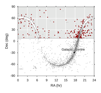
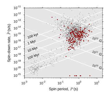
Figure 1: Left: Distribution of all known pulsars from the ATNF pulsar catalogue (grey dots) and the LOFAR census pulsars (red circles) on the sky in equatorial coordinates. The cuts in declination and Galactic latitude made for the LOFAR census sample are shown as grey lines ($\mathrm{Dec}>8^{\circ}$ and $|\mathrm{Gb}|>3^{\circ}$, respectively). For the full list of selection criteria see Table 1. Right: Distribution of all known pulsars (grey dots) and the LOFAR census pulsars (red circles) on the period–period derivative, $P-\dot{P}$, diagram. Pulsars with an unknown $\dot{P}$ are shown at $\dot{P}\mathrm{=10^{-21}\,s\,s^{-1}}$ in the diagram.

2 Observations and data reduction

2.1 Sample selection

We selected the sample of known radio pulsars from version 1.51 of the ATNF Pulsar Catalogue (Manchester et al. 2005; hereafter “pulsar catalogue”) that met the criteria summarised in Table 1. For some of the pulsars that did not satisfy the positional accuracy we were able to find ephemerides with better positions based on timing observations with the Lovell telescope at Jodrell Bank and the 100-m Robert C. Byrd Green Bank Telescope. Such pulsars were included in the census sample.

In total, 194 pulsars were observed. Figure 1 shows the distribution of census sources on the sky and on the standard period–period derivative ($P-\dot{P}$) diagram.

2.2 Observations

Observations were conducted in February–May 2014 using the HBAs of the LOFAR core stations in the frequency range of 110–188 MHz (project code LC1_003). Complex-voltage data from the stations were coherently summed. The total observing band was split into 400 sub-bands, 195 kHz each. Each sub-band was additionally split into 32$-$256 channels and full-Stokes samples were recorded in PSRFITS format (Hotan et al., 2004), with time resolution of 163.84$-$1310.72 $\upmu$s, depending on the number of channels in one sub-band. Larger number of channels was chosen for pulsars with higher DMs in order to mitigate the intra-channel dispersive smearing. For a more detailed description of LOFAR and its pulsar observing modes, we refer a reader to van Haarlem et al. (2013) and Stappers et al. (2011).

Each pulsar was observed during one session for either 1000 spin periods, or at least 20 min. The PSRFITS data were subsequently stored in the LOFAR Long-Term Archive. Observations were pre-processed with the standard LOFAR pulsar pipeline (Stappers et al., 2011), which uses the PSRCHIVE software package (Hotan et al., 2004; van Straten et al., 2010). The data were dedispersed and folded with ephemerides either from the pulsar catalogue or the timing observations with the Lovell or Green Bank telescopes. For the Crab pulsar, we used the Jodrell Bank Crab monthly ephemeris (Lyne et al., 2015). For folding the data, we chose the number of phase bins to be equal to the power of two that matched the original time resolution most closely (but not exceeding 1024). Sometimes, in order to increase the signal-to-noise (S/N) ratio, the number of bins was reduced by a factor of two, four or eight. For all pulsars, the smearing in one channel due to incoherent dedispersion was less than one profile bin at the centre of the band and less than 2.5 bins for the lowest frequency channel. Folding produced 1-min sub-integrations and the archives were averaged in frequency to 400 channels. In this paper we focus only on total intensity data.

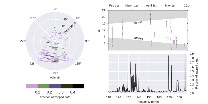
Figure 2: Left: Fraction of zero-weighted data calculated according to Eq. 1 as a function of zenith angle and azimuth of a source. Each stripe corresponds to a single session. Pulsars were observed close to transit and the North celestial pole at the LOFAR core has a zenith angle of approximately $48\degree$. Low-altitude observations are not necessarily more corrupted by RFI and the interference does not come from any preferable azimuth, though the statistics here are limited. Right, top: RFI fraction as a function of Universal Time (UT) and date. Colour coding is the same as on the left subplot. The RFI situation changes rapidly from one observation to another, likely due to the beamed nature of terrestrial signals. Right, bottom: Fraction of zero-weighted data versus observing frequency in each of 400 sub-bands.

2.3 RFI excision

The 77 hours of census observations sampled radio signals from various on-sky directions during both day and night. This makes these data suitable for exploring RFI (radio frequency interference: any kind of unwanted signals of non-astrophysical origin) environment on the site of the LOFAR core stations.

A selective analysis of small random subsets of data, performed with the rfifind program from the PRESTO software package (Ransom, 2001), showed that the majority of RFI was shorter than one minute in duration and/or narrower in frequency than a 195-kHz sub-band (see also Offringa et al., 2013). The real-time excision of RFI, however, was not possible on the full time- and frequency-resolution data due to limited computing power, and thus was performed on folded archives with 1-min sub-integrations and 195-kHz sub-bands. To clean the data we used the clean.py tool from the CoastGuard package (Lazarus et al., 2016).

In general, the observations were not severely affected by RFI. The median fraction of data, zero-weighted due to RFI, was only 5%. This was calculated using:

$$\mathrm{\frac{N_{RFI}}{N_{\text{sub-int}}\times N_{\text{sub-band}}},}$$ (1)

where $\mathrm{N_{RFI}}$ is the number of the zero-weighted [sub-integration, sub-band] cells, and $\mathrm{N_{\text{sub-int}}}$ and $\mathrm{N_{\text{sub-band}}}$ are the total numbers of sub-integrations and sub-bands for each observation. Twelve observing sessions had more than 20% of the data zero-weighted, with the maximum RFI fraction equal to 46%. The fraction of zero-weighted data may vary dramatically between two consecutive sessions. Most census observations were conducted during the daytime, however we did not notice any improvement in the RFI situation during the night. RFI did not appear to come from any specific altitude or azimuth (Fig. 2).

Figure 2 (bottom right) shows also the fraction of zero-weighted data versus observing frequency. Individual noisy sub-bands in this frequency range are likely to be affected by air-traffic control systems, the Dutch emergency paging system C2000, satellite signals and digital audio broadcasting (for the specific list of frequencies, see Table 1 in Offringa et al., 2013).

2.4 Detection and ephemerides update

For most of our pulsars the epoch of observation lay outside the validity range of the available ephemerides. Thus, we expected the observed pulsar period, $P$, and DM to be somewhat different from the values predicted by the ephemerides. We performed initial adjustment of $P$ and DM with the PSRCHIVE program pdmp, which maximises integrated S/N of the frequency- and time- integrated average profile over the set of trial values of $P$ and DM. The output plots from pdmp (namely, maps of integrated S/N values versus trial parameters together with time-integrated spectra and frequency-integrated waterfall plots) were visually inspected for a pulsar-like signal. Out of 194 census pulsars, 158 were detected in such a manner, all with integrated S/N greater than 8. For detected pulsars, pdmp DMs were used to make a template profile and subsequently improve $P$ and DM estimates with the tempo2 timing software (Hobbs et al., 2006) in tempo1 emulation mode. In most cases the new values of $P$ found by tempo2 were very similar to the initial periods. The difference between the new and initial values of $P$, $\delta P$, was in most cases smaller than 5 times the new period error ($\epsilon_{P}$, reported by tempo2 from the least-squares fit). For three moderately bright pulsars, with integrated S/N between 14 and 50, $\delta P$ ranged from seven to $20\epsilon_{P}$. For the bright (integrated S/N of about 500) binary pulsar PSR B0655$+$64 $\delta P$ was as large as $290\epsilon_{P}$.

3 Dispersion measures

Owing to the relatively low observing frequencies and the large fractional bandwidth, for most of the detected pulsars (except for a few faint ones with broad profiles) we were able to measure DMs much more precisely than previous measurements in the pulsar catalogue: our median DM error (provided by tempo2) is 0.0015 pc cm^-3, whereas for the same pulsars the median DM uncertainty in the pulsar catalogue is 0.025 pc cm^-3 (see Table LABEL:table:main for both measured and catalogue DMs). The median relative difference between census DMs and the ones from the pulsar catalogue was $|\delta\mathrm{DM}|/\mathrm{DM}=0.18\%$. However, for a few pulsars the relative DM correction was $\gtrsim 0.1$, and, in the most extreme case of PSR J1503+2111, the pulsar was detected at a DM 3.6 times lower than the previously published value (see Sect. 3.2).

We note that at our level of DM measurement precision a Doppler shift of the observed radio frequency, caused by Earth’s orbital motion should be taken into account. This effect, if not corrected for, would cause an apparent sinusoidal annual DM variation with a relative amplitude of $|\delta\mathrm{DM}/\mathrm{DM}|\lesssim|\varv_{\mathrm{orb}}/c|\approx 0.01\%$, where $\varv_{\mathrm{orb}}$ is the Earth’s orbital velocity. DM measurements can also be biased by profile evolution (intrinsic or caused by scattering, see also discussion in Sect. 3.1), but accounting for profile evolution is beyond the scope of this work.

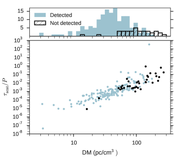
Figure 3: Detected pulsars (light blue dots) and non-detected ones (black dots) versus DM and the scattering time at 150 MHz divided by each pulsar’s period. Scattering time at 1 GHz was taken from the pulsar catalogue (if available) or from the NE2001 model and scaled to 150 MHz with Kolmogorov index of $-4.4$. See the text for the discussion of outliers.

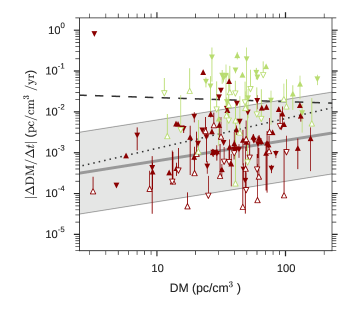
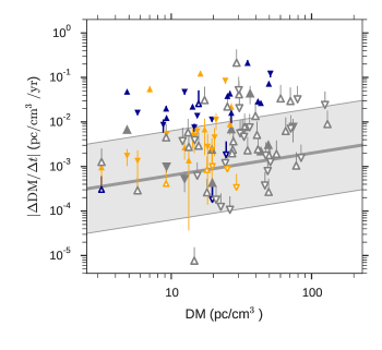
Figure 4: DM variation rates versus census DMs. On both panels the upward/downward triangles indicate DM values increasing/decreasing with time. Unfilled triangles mark pulsars without significant DM variation rate (i. e. with $|\Delta\mathrm{DM}/\Delta t|$ smaller than its uncertainty). For such pulsars the lower parts of the errorbars are not shown. Left: DM variation rates, obtained by comparing census DM measurements to the pulsar catalogue values. Lighter (green) marks show pulsars which have relatively large DM errors ($>0.1$ pc cm^-3), in either the census measurements or the pulsar catalogue. The dotted and dashed lines show unweighted and weighted linear fit to the data in log-log space, respectively, excluding the outlier in the top left corner. The relation of Hobbs et al. (2004b, grey line) is overplotted together with one order-of-magnitude scatter reported by the authors (grey shade). The outlier at $\mathrm{DM}\approx 3$ pc cm^-3, PSR J1503$+$2111 is discussed in Sect. 3.2. Right: Rate of DM variations calculated by comparing census measurements to the recent low-frequency observations of Pilia et al. (2016, larger grey markers), Stovall et al. (2015, dark blue markers) and Zakharenko et al. (2013, light orange markers). See text for discussion.

It is instructive to plot the detections/non-detections versus DM and the expected scattering time over the pulsar period (Fig. 3). The scattering time $\tau_{\mathrm{scat}}$ was scaled to 150 MHz from the values at 1 GHz (obtained from the pulsar catalogue or NE2001 Galactic free electron density model; Cordes & Lazio, 2002) with Kolmogorov index of $-4.4$. As was expected, non-detected pulsars lay mostly at higher DM and $\tau_{\mathrm{scat}}/P$. Still, LOFAR HBAs are capable of detecting non-recycled pulsars up to at least $\mathrm{DM}=180$ pc cm^-3 (PSR B1930+13). Two non-detected pulsars, PSR J2015+2524 and PSR J2151+2315, have small DMs of $<30$ pc cm^-3. They are faint sources and have not been detected at lower frequencies (Camilo & Nice, 1995; Han et al., 2009; Lewandowski et al., 2004; Zakharenko et al., 2013).

One of the pulsars, PSR B2036+53, was detected despite the discouraging predictions of the NE2001 model. This pulsar, located at Galactic coordinates $\mathrm{Gl}=90\aas@@fstack{\circ}37$, $\mathrm{Gb}=7\aas@@fstack{\circ}31$ with a DM of about 160 pc cm^-3, has a predicted $\tau_{\mathrm{scat}}(150\,\mathrm{MHz})=486$ s. The pulsar appeared to show little scattering in the upper half of the HBA band and to have $\tau_{\mathrm{scat}}\approx 0.4$ s at 129 MHz. Moreover, the pulsar has been previously detected with the LPA telescope (Pushchino, Russia) at frequencies close to 100 MHz (Malov & Malofeev, 2010). In NE2001 a region of intense scattering has been explicitly modelled in the direction towards PSR B2036+53. This decision was based on higher-frequency scattering measurements for this pulsar, although the authors neither quote them directly, nor point to the profile data. The average profile at 1408 MHz from Gould & Lyne (1998), available via the EPN, seems to show a small scattering tail, with $\tau_{\mathrm{scat}}$ approximately in agreement with NE2001. However, both the S/N and the time resolution of the 1408 MHz profile are not high. Being extrapolated down to 700 MHz with the Kolmogorov index, $\tau_{\mathrm{scat}}$ from NE2001 would have caused an order of magnitude larger profile broadening than was observed by Gould & Lyne (1998) and Han et al. (2009). It is, therefore, possible that modelling the region of intense scattering towards this pulsar is not necessary. For comparison, the scattering time from the Taylor & Cordes (1993) Galactic electron density model is equal to 40 ms at 129 MHz (scaled from 1 GHz with Kolmogorov index). This model does not include the region of intense scattering towards PSR B2036+53 and the predicted scattering time is much closer to the measured value.

3.1 DM variations

Because of the relative motion of the pulsar/ISM with respect to an Earth-based observer, the DM along any given line of sight (LOS) will gradually change with time. Systematic monitoring of DMs reveals that, in general, $\mathrm{DM}(t)$ series consist of slowly varying (i.e. approximately linear) components superposed with stochastic or periodic variations (Keith et al., 2013; Coles et al., 2015). The interpretation of these variations can cast light on the turbulence in the ionised electron clouds in the interstellar plasma (Armstrong et al., 1995), though the interpretation may be more complex than usually assumed (Lam et al., 2016).

Due to the high precision achievable for each single DM measurement, low-frequency DM monitoring can be particularly useful for investigating small, short-term DM variations. Within the census project, however, the DM along any particular LOS was measured only once. Nevertheless, some crude estimates on the DM variation rates can be obtained by comparing census DMs with previously published values.

We calculated the rate of DM variation for the census pulsars by comparing their DMs to those obtained from the pulsar catalogue:

$$|\Delta\mathrm{DM}/\Delta t|=\left|\frac{\mathrm{DM_{cat}}-\mathrm{DM_{cen}}}{(\mathrm{DMepoch_{cat}}-\mathrm{DMepoch_{cen}})/365.25}\right|,$$ (2)

where the epochs of DM measurements were expressed in MJD. The errorbars were set by the error of DM determination:

$$\epsilon_{|\Delta\mathrm{DM}/\Delta t|}=\frac{\sqrt{\epsilon^{2}_{\mathrm{DM_{cat}}}+\epsilon^{2}_{\mathrm{DM_{cen}}}}}{\left|\mathrm{DMepoch_{cat}}-\mathrm{DMepoch_{cen}}\right|/365.25},$$ (3)

and the pulsars without records of DM uncertainties or DM epochs in the pulsar catalogue were excluded from the sample. This resulted in a sample of 146 pulsars, with DMs between 3 and 180 pc cm^-3, and 5–30 years between the catalogue and census measurement epochs.

We have compared our results to a similar study in Hobbs et al. (2004b), who measured the rate of DM variations for about 100 pulsars with DMs between 3 and 600 pc cm^-3. Their analysis was based on 6–34 years of timing data, taken mostly at 400$-$1600 MHz. Figure 4 (left) shows $|\Delta\mathrm{DM}/\Delta t|$ versus DM for census observations together with the approximate spread of $|\Delta\mathrm{DM}/\Delta t|$ values from Hobbs et al. (2004b). Most of our pulsars have rates of DM variation similar to the ones from Hobbs et al. (2004b). However, there are some deviations: the nearby PSR J1503+2111 exhibits unusually large $|\Delta\mathrm{DM}/\Delta t|=0.8$ pc cm^-3 $\mathrm{yr^{-1}}$ (see Sect. 3.2) and there is an excess of larger DM variations for pulsars with $\mathrm{DM}>10$ pc cm^-3. It is interesting to note that pulsars with larger DM variation rates have relatively large reported DM errors: $\epsilon_{\mathrm{DM}}>0.1$ pc cm^-3, mostly for the pulsar catalogue DMs. Although DM uncertainties are explicitly included in the error bars in Fig. 4, it is possible that some of the DM measurements have unaccounted systematic errors, with a probability of such error underestimation being larger for pulsars with larger quoted $\epsilon_{\mathrm{DM}}$ (e.g. because of low S/N of the profile).

In addition, we must note that census DM measurements were obtained under the simplifying assumption of the absence of profile evolution within the HBA band. It is currently unclear how different profile evolution models would affect the measured DM values. As a very approximate estimate, allowing the fiducial point to drift by 0.01 in spin phase (10% of the typical width of an average pulse) across the HBA band would lead to a median DM change of 0.03 pc cm^-3, 20 times larger than the median DM precision. This would alter the observed $|\Delta\mathrm{DM}/\Delta t|$ typically by about 0.002 pc cm^-3 $\mathrm{yr^{-1}}$, but for some pulsars the change could be as large as 0.01 pc cm^-3 $\mathrm{yr^{-1}}$.

Investigating the dependence of DM variation rate on DM can provide basic information for simple models of interstellar plasma fluctuations. Backer et al. (1993), based on a sample of 13 pulsars with DMs between 2 and 200 pc cm^-3, have found that $|\Delta\mathrm{DM}/\Delta t|\sim\sqrt{\mathrm{DM}}$, which motivated the authors to propose a wedge model of electron column density gradients in the ISM. Hobbs et al. (2004b) found a similar dependence:

$$|\Delta\mathrm{DM}/\Delta t|\approx 0.0002\times\mathrm{DM}^{0.57\pm 0.09}_{\mathrm{pc\,cm^{-3}}}\quad\mathrm{pc\,cm^{-3}\,yr^{-1}}.$$ (4)

Both Backer et al. (1993) and Hobbs et al. (2004b) note a large (order of magnitude) scatter of data points around the fitted relation. At least partially, this scatter may be due to the dispersion in pulsar transverse velocities, since $|\Delta\mathrm{DM}/\Delta t|$ depends also on the transverse velocity of a pulsar.

For the census data, the unweighted fit of the following function:

$$\lg|\Delta\mathrm{DM}/\Delta t|_{\mathrm{pc\,cm^{-3}\,yr^{-1}}}=\lg A+B\lg\mathrm{DM_{pc\,cm^{-3}}},$$ (5)

resulted in a relation which was close to Hobbs et al. (2004b), with $B=0.7\pm 0.2$ and $A\approx 0.0002$  ($\lg A=-3.6\pm 0.4$). Assigning each $|\Delta\mathrm{DM}/\Delta t|$ a weight inversely proportional to the measurement uncertainty yielded a fit with $B=-0.1\pm 0.1$ and $A\approx 0.03$ ($\lg A=-1.5\pm 0.2$), however the usefulness of this approach is limited since the contribution from the transverse velocities and possible measurement bias due to profile evolution are not taken into account. Excluding the insignificant (value smaller than the error) $|\Delta\mathrm{DM}/\Delta t|$ or the ones with $\epsilon_{\mathrm{DM}}>0.1$ pc cm^-3  did not affect the fitting results substantially, except for when PSR J1503+2111 was included.

Overall, it is hard to make any definitive conclusion about the relation between $|\Delta\mathrm{DM}/\Delta t|$ and DM based on census data. Future improvements may result from extending the sample to larger DMs, including more pulsars with $\mathrm{DM}<10$ pc cm^-3, making DM($t$) measurements with the same profile model, better quantification of DM gradients (e.g. separating piecewise linear segments and removing contributions of stochastic or periodic variations), and accounting for the contribution from transverse velocities.

Besides the pulsar catalogue, we compared the census DMs to recently published DM measurements taken within the last five years at frequencies less than or equal to HBA frequencies (Pilia et al., 2016; Stovall et al., 2015; Zakharenko et al., 2013). Pilia et al. (2016) observed 100 pulsars with the LOFAR HBA antennas approximately two years before the census observations presented here. At this time of data acquisition, just over half of the current HBA band and fewer core stations were available in tied-array mode, resulting in lower (by a factor of a few) S/N in the average profiles and larger errors in DM determination. The other two works report DMs measured at frequencies below 100 MHz. Zakharenko et al. (2013) observed nearby ($\mathrm{DM}<30$ pc cm^-3) pulsars in the frequency range of 16.5–33 MHz using the UTR-2 telescope. Observations were taken during three sessions in 2010–2011. The authors do not specify the exact epoch of DM measurements, so the inferred uncertainty of DMepoch is included in errors on $|\Delta\mathrm{DM}/\Delta t|$ in Fig. 4. Stovall et al. (2015) report the results of broadband (35–80 MHz) pulsar observations with the LWA telescope. Their DM measurements were taken close in time to the census ones: the maximum offset between the DM epochs was about $\pm 1$ yr. Some of the census pulsars were observed in more than one of these three works, thus they have multiple $|\Delta\mathrm{DM}/\Delta t|$ plotted in Fig. 4 (right). The calculated DM variation rates for such pulsars could differ from each other by one-two orders of magnitude.

In general, DMs from at least two aforementioned works also suggest the excess of larger DM variation rates as comparing to Hobbs et al. (2004b). This trend is the most obvious for the shortest timespan $|\Delta\mathrm{DM}/\Delta t|$ based on DMs from Stovall et al. (2015). The fact that DM variation rates are larger on smaller timescales can be explained by the larger relative influence of shorter-term stochastic variations. However, the bias in $|\Delta\mathrm{DM}/\Delta t|$ introduced by DM offsets due to the differences in modelling the frequency-dependent profile evolution and scattering will also be relatively larger because of the shorter time span in the denominator of Eq. 2.

Making DM measurements in the presence of profile evolution and scattering is a complex task (Hassall et al., 2012; Pennucci et al., 2014; Liu et al., 2014). Nevertheless, this provides valuable information about both the ISM (electron content and turbulence parameters) and pulsar magnetospheres (such as modelling the location of a fiducial phase point and the evolution of components around it; e.g. Hassall et al. 2012). Scattering has a steep dependence on frequency, and profile evolution is usually more rapid at lower frequencies. Thus, combining census observations with lower frequencies (or even with higher-frequency data for pulsars with large scattering times) can serve as a good data sample for broadband profile modelling, bias-free DM measurements, and scattering time estimates. Finally, it would be interesting to investigate frequency dependence of DM values, arising from different sampling of the ISM, due to frequency-dependent scattering (Cordes et al., 2016). We will defer such analysis to a subsequent work.

3.2 PSR J1503$+$2111

PSR J1503$+$2111 exhibited an unusually large DM variation rate of about $-0.8$ pc cm^-3$\mathrm{yr^{-1}}$. It has $\mathrm{DM_{cat}}=11.75\pm 0.06$ pc cm^-3 (Champion et al., 2005a) and $\mathrm{DM_{cen}}=3.260\pm 0.004$ pc cm^-3, with measurements taken 11 yr apart. In our observations, folded with $\mathrm{DM_{cat}}$, the pulsar is clearly visible across the entire HBA band and its profile exhibits a characteristic quadratic sweep with a net delay between the edges of the band equal to 0.6 of spin phase. Thus, we are confident that at the epoch of census observation the DM of PSR J1503$+$2111 was substantially different from $\mathrm{DM_{cat}}$.

PSR J1503$+$2111 was discovered only a decade ago and is relatively poorly studied. The DM value in the pulsar catalogue comes from the discovery paper of Champion et al. (2005a). The authors obtained initial ephemerides (including DM) based on 430-MHz timing data taken with the Arecibo telescope. They subsequently refined the DM using observations at four frequencies between 320 and 430 MHz, while keeping other ephemeris parameters fixed. If the real DM value was close to 3 pc cm^-3 at the time of observations, then the time delay from the highest to the lowest frequencies in their setup would be around $-150$ ms (0.04 of spin phase), much larger than the reported residual time-of-arrival rms of 0.9 ms. However, such DM error could pass unnoticed while folding observations within one band ($-7$ ms delay, about 10% of pulse width reported). The pulsar was subsequently observed by Han et al. (2009), in a frequency band spanning from 726 to 822 MHz. At these frequencies the profile smearing due to incorrect DM would be only 0.004 of spin phase, much smaller than the profile width (0.03 of spin phase) presented in their work. Zakharenko et al. (2013) failed to detect PSR J1503$+$2111 at 16–33 MHz, searching for a pulsar signal with a set of trial DM values within 10% of $\mathrm{DM_{cat}}$. If the DM at the epoch of Zakharenko et al. (2013) observations was close to 3.26 pc cm^-3, the delay due to the DM offset at their frequencies would be equal to 30 phase wraps, completely smearing the profile.

To summarise, it is possible that the DM of this pulsar was incorrectly estimated in Champion et al. (2005a) and went unnoticed since then. However, only future observations of this pulsar can show whether the DM along this LOS exhibits an anomalously large variation rate.

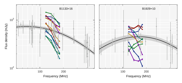
Figure 5: Flux density measurements from individual timing sessions ($S_{\mathrm{meas}}$, coloured connected dots) for two out of the ten pulsars used for flux density uncertainty estimates. Separate grey dots are flux density values from the literature, with the errors estimated according to the procedure described in Sect. 5.2. The black line indicates $S_{\mathrm{lit}}$, the parabola fit for literature flux density points within 10$-$1000 MHz. The shaded region marks 68% uncertainty on $S_{\mathrm{lit}}$.

4 Flux density calibration

4.1 Overview and error estimate

The flux density scale for a given [sub-integration, sub-band] cell was calibrated with the radiometer equation (Dicke, 1946):

$$S_{\mathrm{mean}}=\dfrac{T_{\mathrm{sys}}}{G\sqrt{n_{p}\Delta ft_{\mathrm{obs}}n^{-1}_{\mathrm{bin}}}}\times\langle\mathrm{S/N}\rangle,$$ (6)

where $T_{\mathrm{sys}}=T_{\mathrm{A}}+T_{\mathrm{sky}}$ is the total system temperature (antenna plus sky background), $G$ is the telescope gain, $n_{p}$ is the number of polarisations summed (2 for census data), $\Delta f$ is sub-band width, $t_{\mathrm{obs}}$ is the length of sub-integration, $n_{\mathrm{bin}}$ is the number of spin phase bins, and $\langle\mathrm{S/N}\rangle$ is the mean signal-to-noise ratio of the pulse profile in a given [sub-integration, sub-band] cell. For LOFAR, both antenna temperature and gain have a strong dependence on frequency, with the latter also varying with the elevation and azimuth of the source observed. In this work we used the latest version of the LOFAR pulsar flux calibration software, described in Kondratiev et al. (2016). This software uses the Hamaker beam model (Hamaker, 2006) and mscorpol package by Tobia Carozzi to calculate Jones matrices of the antenna response for a given HBA station, frequency and sky direction. The antenna gain is further scaled with the actual number of stations used in a given observation. The HBA antenna temperature, $T_{\mathrm{A}}$, is approximated as a frequency-dependent polynomial derived from the measurements of Wijnholds & van Cappellen (2011). The background sky temperature, $T_{\mathrm{sky}}$, is calculated using 408-MHz maps of Haslam et al. (1982), scaled to HBA frequencies as $\nu^{-2.55}$ (Lawson et al., 1987). The mean S/N of the pulse profile is calculated by averaging the normalised signal over the pulse period, with the normalisation performed using the mean and standard deviation of the data in the manually selected off-pulse window (the region in pulse phase without visible emission). Zero-weighted sub-bands and/or sub-integrations are ignored and do not contribute to the overall flux density calculation. For a more detailed review of the calibration technique we refer the reader to Kondratiev et al. (2016).

The nominal error on the flux density estimation in Kondratiev et al. (2016), $\epsilon_{S\mathrm{nom}}$, is set by the standard deviation of the data in the off-pulse window. The real uncertainty of a single flux density measurement is much larger, being augmented by many factors, including (but not limited to) the intrinsic variability of the source, scintillation in the ISM, imperfect knowledge of the system parameters, and some other possible effects that are unaccounted for, e.g. uncalibrated phase delays introduced by the ionosphere or the presence of strong sources in the sidelobes.

To provide a more realistic uncertainty, we took advantage of regular LOFAR pulsar timing observations. Within this project, a number of both millisecond and normal pulsars were observed with HBA core stations on a monthly basis. From this sample of pulsars we selected ten bright non-recycled pulsars with relatively well-known spectra available from the literature. These pulsars were observed for 5–20 min at different elevations and azimuths in December 2013–November 2014, approximately in the same time span as the census observations. The distribution of LOS directions approximately coincides with that for the census pulsars. In particular, both timing and census sources were observed only at relatively high elevations (EL), $\mathrm{EL>40}^{\circ}$.

Table 2: Percentiles of $S_{\mathrm{lit}}/S_{\mathrm{meas}}$ distribution for ten bright pulsars with HBA timing observations.

	4 sub-bands				2 sub-bands		band-integrated
	120 MHz	139 MHz	159 MHz	178 MHz	130 MHz	168 MHz	149 MHz
median	0.8	1.0	1.0	1.2	0.9	1.1	1.0
16th percentile	0.5	0.6	0.6	0.6	0.6	0.6	0.6
84th percentile	1.5	1.6	1.7	2.2	1.5	1.9	1.6

We processed selected timing observations and measured the pulsar flux densities in the same manner as for census sources. Examination of the flux density values obtained revealed two to four times larger fluctuations than would have been expected by scintillation alone, with a flux density rms on the order of 50% for the band- and session-integrated flux densities. This is at least partly due to the imperfect model of telescope gain, since we record a dependence of the measured flux density on the source elevation. The number of flux density measurements, however, is too small to construct a robust additional gain correction. Thus, we leave it for future work.

Figure 5 shows measured spectra with respect to literature points for two pulsars from the timing sample. In order to estimate the error of a single flux density measurement (and check for any systematic offsets between LOFAR and literature flux densities), we constructed a “reference” flux density curve $S_{\mathrm{lit}}$ by fitting a parabola to the literature flux density values in logarithmic space (within the range 10$-$1000 MHz). The fit was performed using a Markov chain Monte-Carlo (MCMC) algorithm and the region between 16th and 84th percentiles of $S_{\mathrm{lit}}$ values (obtained from posterior distributions of the fitted parabola parameters) is shown with a grey shade. This formal uncertainty in $S_{\mathrm{lit}}$ should be treated as an approximation of the actual uncertainty, since the fitted curve can shift by an amount larger than the grey-shaded area if new flux density measurements are added. We then analysed the distribution of $S_{\mathrm{lit}}/S_{\mathrm{meas}}$ values, where the flux density obtained from timing observations, $S_{\mathrm{meas}}$, is in the denominator. For band-integrated flux densities, the median value of $S_{\mathrm{lit}}/S_{\mathrm{meas}}$ was 1.0 and $0.6<S_{\mathrm{lit}}/S_{\mathrm{meas}}<1.6$ with 68% probability.

Thus, for the sample of ten timing pulsars the combined influence of all uncertainties, other than $\epsilon_{S\mathrm{nom}}$ caused $S_{\mathrm{meas}}$ to spread around $S_{\mathrm{lit}}$ with a magnitude of the spread equal to about $0.5S_{\mathrm{meas}}$. Assuming the uncertainties to be similar for all census pulsars, we adopted a total error on the single flux density measurement $\epsilon_{S}=\sqrt{(0.5S)^{2}+\epsilon_{S\mathrm{nom}}^{2}}$. This assumption is reasonable, since we expect two major contributors to the flux density uncertainty, namely, our imperfect knowledge of the gain and interstellar scintillation, to influence both timing and census observations to a similar extent. This is justified because the distribution of source elevations and expected modulation indices due to scintillation (see Appendix A for the latter) were similar for both timing and census sources.

We also examined the error distribution for flux densities measured in halves and quarters of the HBA band. We discovered that, in general, the slopes of the timing spectra are inconsistent with the literature, with lower-frequency $S_{\mathrm{meas}}$ being consistently overestimated and higher-frequency $S_{\mathrm{meas}}$ underestimated (see Table 2).

Two alternative models of antenna gain were also tested. The first model was based on full electromagnetic simulations of an ideal 24-tile HBA sub-station including edge effects and grating lobes (Arts et al., 2013). The second model used a simple $\sim\sin^{1.39}(\mathrm{EL})$ scaling of the theoretical frequency-dependent value of the antenna effective area (Noutsos et al., 2015). For both models the telescope gain at zenith was similar to the Hamaker-Carozzi model, but they predict two to three times larger gains for the lowest census elevations of $40\degree$. This meant that pulsar flux densities could be two to three times smaller than those calculated using the Hamaker-Carozzi model, which made them less consistent with $S_{\mathrm{lit}}$ values.

For several bright pulsars we also estimated the preliminary 140-MHz flux densities using images from the Multifrequency Snapshot Sky Survey (G. Heald, private communication; see also Heald et al., 2015). The same technique was applied to compare the imaging flux density values, $S_{\mathrm{MSSS}}$, and $S_{\mathrm{lit}}$. We found that 16th–84th percentiles of $S_{\mathrm{MSSS}}$ agree with $S_{\mathrm{lit}}$ within 40%, similarly to the flux densities from the timing campaign.

4.2 Application to census pulsars

The flux density calibration was performed on folded, 195-kHz-wide, 1-min sub-integrations. In addition to the synchrotron background from Haslam et al. (1982), we have checked for any bright sources in the primary beam. In all cases the Sun, the Moon, and the planets were far away ($>4\aas@@fstack{\circ}7$) from a pulsar position. A review of the 3C and 3CR catalogues (Edge et al., 1959; Bennett, 1962) did not reveal any nearby extended sources, except in the case of the Crab pulsar (3C144) and PSR J0205$+$6449 (3C58). For the Crab pulsar, the contribution from the nebula was estimated with the relation $S_{\mathrm{Jy}}\approx 955\nu_{\mathrm{GHz}}^{-0.27}$ (Bietenholz et al., 1997; Cordes et al., 2004). Similar flux density values were quoted in the 3C catalogue. At 75 MHz, the solid angle occupied by the nebula (radius of $4\arcmin$, Bietenholz et al., 1997) is larger than the full-width at the half-maximum of the LOFAR HBA beam ($2\arcmin$, for the 2-km baseline, according to the table B.2 in van Haarlem et al., 2013), thus only approximately one quarter of the nebula is contributing to the system temperature. For PSR J0205$+$6449, the supernova remnant does not significantly add to the system temperature (5–10%, depending on the observing frequency), so its contribution was neglected.

For all pulsars, except for the Crab, we were able to find an off-pulse region in each sub-band/sub-integration, although in some cases the off-pulse region was small (about 10% of pulse phase). Sometimes the band- and time-integrated average profile exhibited faint pulsed emission in the selected off-pulse region, resulting in somewhat underestimated flux densities. However, because of the large number of channels and sub-integrations in our observing setup (400 and $\geqslant 20$, respectively), we expect this underestimation to be well within the quoted errors. For the Crab pulsar, the standard deviation of the noise was calculated after subtracting a polynomial fit to the profile.

The band-integrated flux density values, together with the adopted uncertainties $\epsilon_{S}$ are quoted in Table LABEL:table:main. For non-detected pulsars we give $3\epsilon_{S\mathrm{nom}}$ as an upper limit. We note that such upper limits must be taken with caution, since non-detections can occur for reasons unrelated to the intrinsic pulsar flux density (for example, scattering or unknown error in the pulsar position).

5 Spectra

5.1 Introduction

The mean (averaged over period) flux density $S_{\nu}$ of a pulsar observed at a frequency $\nu$ is one of the main observables of pulsar emission. Flux density measurements provide constraints on the pulsar emission mechanism (Malofeev & Malov, 1980; Ochelkov & Usov, 1984). They are crucial for deriving the pulsar luminosity function (which is further used to study the birth rate and initial spin period distribution of the Galactic population of radio pulsars, e.g. Lorimer et al., 1993; Faucher-Giguère & Kaspi, 2006), and for planning the optimal frequency coverage of future pulsar surveys.

At present, even the most well-studied pulsar radio spectra consist of flux density measurements obtained from observations performed under disparate conditions and with different observing setups. The situation is further complicated by interstellar scintillation and intrinsic pulsar variability (Sieber, 1973; Malofeev & Malov, 1980). As a result, flux densities measured at the same frequency by different authors may disagree by up to an order of magnitude.

Despite these difficulties, it has been established that in a wide frequency range of approximately 0.1–10 GHz, pulsar radio spectra are usually well-described by a simple power-law relation:

$$S_{\nu}=S_{0}\left(\nu/\nu_{0}\right)^{\alpha},$$ (7)

where $S_{0}$ is the flux density at the reference frequency $\nu_{0}$, and $\alpha$ is the spectral index. At the edges of this frequency range some spectra start deviating from a single power-law, exhibiting a so-called low-frequency turnover at $\lesssim 100$ MHz (Malofeev, 1993), or high-frequency flattening around 30 GHz (Kramer et al., 1996). Some pulsars show evidence of a spectral break even in the centimetre wavelength range (Maron et al., 2000) and there is a subclass of pulsars with distinct spectral turnover around 1 GHz (Kijak et al., 2011).

Based on the extensive number of published flux density measurements (see Table LABEL:table:main for the full list of references), we constructed radio spectra for 182 census pulsars (Figs. LABEL:fig:spectra_nondet–LABEL:fig:prof_sp_16). Among those spectra, 24 consisted of the literature points only, since the corresponding pulsars were not detected in census observations. Twelve remaining pulsars were not detected in the census observations and had no previously published flux density values.

5.2 Fitting method

It is customary to fit pulsar spectra with a single or broken power-law (PL), although this approach may be only an approximation to the true pulsar spectrum (Maron et al., 2000; Löhmer et al., 2008). Still, this parametrisation is useful for cases with a limited number of measurements and allows direct comparison to previous work.

The fit was performed in $\lg S$–$\lg\nu$ space. We used a Bayesian approach, making a statistical model of the data and using an MCMC fitting algorithm to find the posterior distributions of the fitted parameters. In general, we modelled each $\lg S$ as a normally distributed random variable with the mean $\lg S_{\mathrm{PL}}$ defined by the PL dependence and a standard deviation $\sigma_{\lg S}$ reflecting any kind of flux density measurement uncertainty:

$$\lg S\sim\mathrm{Normal}(\lg S_{\mathrm{PL}},\sigma_{\lg S}).$$ (8)

A normal distribution was chosen for the sake of simplicity and for the lack of a better knowledge of the real uncertainty distribution.

Depending on the number of flux density measurements and their frequency coverage, $\lg S_{\mathrm{PL}}$ was approximated either as a single PL (hereafter “1PL”):

$$\lg S_{\mathrm{1PL}}=\alpha\lg(\nu/\nu_{0})+\lg S_{0},$$ (9)

a broken PL with one break (2PL):

$$\lg S_{\mathrm{2PL}}=\begin{cases}\alpha_{\mathrm{lo}}\lg(\nu/\nu_{0})+\lg S_{0},&\nu<\nu_{\mathrm{br}}\\ \alpha_{\mathrm{hi}}\lg(\nu/\nu_{\mathrm{br}})+\alpha_{\mathrm{lo}}\lg(\nu_{\mathrm{br}}/\nu_{0})+\lg S_{0},&\nu>\nu_{\mathrm{br}},\end{cases}$$ (10)

or a broken PL with two breaks (3PL):

$$\lg S_{\mathrm{3PL}}=\begin{cases}\alpha_{\mathrm{lo}}\lg(\nu/\nu_{0})+\lg S_{0},&\nu<\nu^{\mathrm{lo}}_{\mathrm{br}}\\ \alpha_{\mathrm{mid}}\lg(\nu/\nu^{\mathrm{lo}}_{\mathrm{br}})+\alpha_{\mathrm{lo}}\lg(\nu^{\mathrm{lo}}_{\mathrm{br}}/\nu_{0})+\lg S_{0},&\nu^{\mathrm{lo}}_{\mathrm{br}}<\nu<\nu^{\mathrm{hi}}_{\mathrm{br}}\\ \alpha_{\mathrm{hi}}\lg(\nu/\nu^{\mathrm{hi}}_{\mathrm{br}})+\alpha_{\mathrm{mid}}\lg(\nu^{\mathrm{hi}}_{\mathrm{br}}/\nu_{0})+\lg S_{0},&\nu>\nu^{\mathrm{hi}}_{\mathrm{br}}.\end{cases}$$ (11)

For all PL models, the reference frequency $\nu_{0}$ was taken to be the geometric average of the minimum and maximum frequencies in the spectrum, rounded to hundreds of MHz.

If the number of spectral data points was small (two to four, with measurements within 10% in frequency treated as a single group), we fixed $\sigma_{\lg S}$ at the known level, defined by the reported errors: $\sigma_{\lg S}\equiv\sigma^{\mathrm{kn}}_{\lg S}=0.5[\lg(S+\epsilon^{\mathrm{up}}_{S})-\lg(S-\epsilon^{\mathrm{lo}}_{S})]$. For census measurements the errors were taken from Table 2 and added in quadrature to $\epsilon_{S\mathrm{nom}}$. The errors on the literature flux densities were assigned following the essence of the procedure described in Sieber (1973).

When the number of data points was larger (more than six or, sometimes, five groups), we introduced an additional fit parameter, the unknown error $\sigma^{\mathrm{unkn}}_{\lg S}$. This error represents any additional flux density uncertainty, not reflected by $\sigma^{\mathrm{kn}}_{\lg S}$, for example intrinsic variability, or any kind of unaccounted propagation or instrumental error. The total flux density uncertainty of any measurement was then taken as the known and unknown errors added in quadrature. We fit a single $\sigma^{\mathrm{unkn}}_{\lg S}$ per source, although, strictly speaking, unknown errors may be different for each separate measurement.

In the presence of a fitted $\sigma^{\mathrm{unkn}}_{\lg S}$ all three PL models will provide a good fit to the data, since any systematic deviation between the model and the data points will be absorbed by $\sigma^{\mathrm{unkn}}_{\lg S}$. Thus, in order to discriminate between models, we examined the posterior distribution of $\sigma^{\mathrm{unkn}}_{\lg S}$. We took 1PL as a null hypothesis and rejected it in favour of 2PL or 3PL if the latter gave statistically smaller $\sigma^{\mathrm{unkn}}_{\lg S}$: the difference between the mean values of the posterior distributions of $\sigma^{\mathrm{unkn}}_{\lg S}$ was larger than the standard deviations of those distributions added in quadrature.

For the sparsely-sampled spectra, where no $\sigma^{\mathrm{unkn}}_{\lg S}$ was fitted, we adopted 1PL as the single model. In a few cases, when the data showed a hint of a spectral break, we fitted 2PL with break frequency fixed at the frequency of the largest flux density measurement. For such pulsars we give both 1PL and 2PL values of the fitted parameters.

Some flux density measurements were excluded from the fit. Since most of the flux density measurements were performed for the pulsed emission, we did not take into account the continuum flux density values for the Crab pulsar at 10–80 MHz from Bridle (1970). For PSR B1133+16 we excluded the measurements from Stovall et al. (2015), since they were an order-of-magnitude larger than numerous previous measurements in the same frequency range. Judging from the visual examination of well-measured spectra, sometimes the upper limit on flux densities could be an order-of-magnitude smaller than actual measurements in the same frequency range. Thus, we considered both census and literature flux density upper limits to be approximate at best and did not attempt to fit for the lower limits on spectral index.

5.3 Results

Out of the 194 census pulsars, 165 had at least two flux density measurements (census or literature), making them suitable for a spectral fit. The majority of pulsars, 124 sources, were well-described with the 1PL model (Table LABEL:table:1pl), although the choice of the model was greatly influenced by the small number of data points available. Four 1PL pulsars (namely PSRs J1238$+$21, J1741$+$2758, B1910$+$20, and J2139$+$2242) show signs of spectral break, but the number of flux density measurements was too small to fit for a break frequency. For these pulsars we provide the values of the 2PL parameters with a break frequency fixed at the frequency of maximum flux density (Table LABEL:table:2pl). The remaining 41 sources showed preference for a broken power-law with a single break (36 pulsars, Table LABEL:table:2pl), or two breaks (five pulsars, Table LABEL:table:3pl). Pulsars best described with a 2PL or 3PL model usually have a larger number of flux density measurements.

5.4 Discussion

5.4.1 Flux variability

It is interesting to examine the distribution of $\sigma^{\mathrm{unkn}}_{\lg S}$ among the pulsars for which this parameter was fitted. The 46 of these sources were best described by the 1PL model. About $60\%$ of them showed moderate flux density scatter with $\sigma^{\mathrm{unkn}}_{\lg S}\lesssim 0.15$, indicating roughly $\pm$30% variation in flux density measurements at a single frequency. Six 1PL pulsars had $\sigma^{\mathrm{unkn}}_{\lg S}>0.3$, with flux density varying by a factor of two to six. Among those, four pulsars (PSRs B0053$+$47, B0450$+$55, B1753$+$52, and J2307$+$2225) had separate outliers in their spectra, hinting at a deviation from the 1PL model, or simply indicating a large unaccounted error in a single flux density measurement. PSRs B0643$+$80 and J1740$+$1000 had a large spread of flux density measurements across the entire spectrum. Interestingly, PSR B0643$+$80 was shown to have burst-like emission in one of its profile components (Malofeev et al., 1998). The other pulsar, PSR J1740$+$1000, was proposed as a candidate for a gigahertz-peaked spectrum pulsar by Kijak et al. (2011), although the authors note contradicting flux density measurements at 1.4 GHz. These contradicting points were excluded from the spectral analysis conducted by Dembska et al. (2014) and Rajwade et al. (2016), who approximated the spectrum of PSR J17400$+$1000 with a parabola or fitted the PL with a free-free absorption model directly. Our measurements show that the flux density of PSR J1740$+$1000 does not decrease at HBA frequencies, exceeding the extrapolation of the fits by Dembska et al. (2014) and Rajwade et al. (2016) by a factor of 10–20. We suggest this pulsar does not have a gigahertz-peaked spectrum, but a regular PL with potentially large flux density variability.

For both 2PL and 3PL pulsars, the median value of $\sigma^{\mathrm{unkn}}_{\lg S}$ was 0.1. Two 2PL pulsars, PSR B0943+10 and PSR B1112+50, had $\sigma^{\mathrm{unkn}}_{\lg S}>0.3$. The former is a well-known mode-switching pulsar (Suleymanova & Izvekova, 1984) and the latter has a 20-cm profile that is unstable on the time scale of our observing session (Wright et al., 1986). This can explain an order-of-magnitude difference between the flux densities obtained from the census measurements and the ones reported by Karuppusamy et al. (2011), which were performed in exactly the same frequency range.

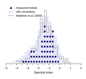
Figure 6: Distribution of spectral indices for 48 pulsars without previously published spectral fits. Each of the 48 dark squares marks the mean of the posterior distribution of the spectral index $\alpha$. The lighter histogram was constructed using the whole posterior distribution of $\alpha$ for all pulsars, and thus reflects the uncertainty in the spectral index determination. The grey line marks the distribution of spectral indices for 175 non-recycled pulsars in the similar frequency range (100–400 MHz) from Malofeev et al. (2000).

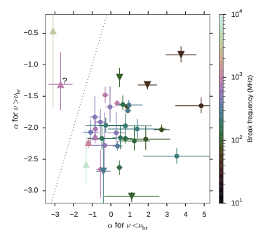
Figure 7: Spectral indices below and above the spectral break for 32 pulsars with relatively well-measured spectra (see text for details). Pulsars with a single spectral break are marked with circles. For pulsars with two spectral breaks, the lower-frequency one is marked with the downward triangles and the higher-frequency one with the upward triangles. The colour indicates the frequency of the break and the dotted line corresponds to no change in the spectral index. The question mark indicates PSR B2303$+$30, for which the value of the high-frequency spectral index was greatly influenced by a single flux density measurement. Note that for $\nu_{\mathrm{br}}\gtrsim 500$ MHz the change in spectral index is relatively moderate, whereas for $\nu_{\mathrm{br}}\lesssim 300$ MHz the spectral index below the break takes (sometimes large) positive values. This corresponds to the previously known “high-frequency cut-off” and “low-frequency turnover” in pulsar spectra.

5.4.2 New spectral indices

In total, 48 pulsars from the census sample did not have previously published spectral fits. The spectra of these pulsars typically consisted of a small ($\lesssim 5$) number of points, usually limited to the frequency range 100 – 400/800 MHz. Among these 48 pulsars, only PSR J2139+2242 showed signs of a spectral break, however the paucity of available measurements should be kept in mind.

The distribution of new spectral indices (Fig. 6) is comparable in shape to the spectral index distribution constructed from a larger sample of 175 non-recycled pulsars in a similar frequency range (between 102.5 and 408 MHz) by Malofeev et al. (2000). Both in Malofeev et al. (2000) and in our work the mean value of the spectral index, $\bar{\alpha}=-1.4$, is flatter than the mean spectral index measured at frequencies above 400 MHz (e.g. $\bar{\alpha}=-1.8$ in Maron et al., 2000). This can be interpreted as a sign of low-frequency flattening or turnover (Malofeev et al., 2000). However, as has been noted by Bates et al. (2013), the shapes of observed spectral index distributions may be greatly affected by the selection effects connected to the frequency-dependent sensitivity of pulsar surveys. Thus, a comparison of spectral index distributions obtained in the different frequency ranges should be done with caution unless the distributions are based on the same sample of sources.

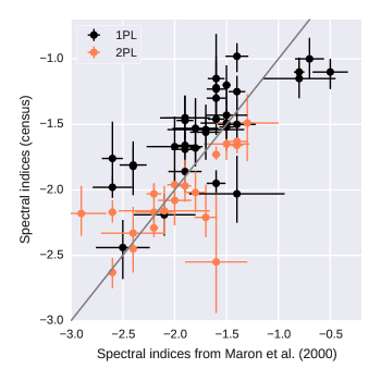
Figure 8: Comparison between spectral indices from Maron et al. (2000) and this work. Black circles indicate 35 pulsars with spectra best described with a single PL by Maron et al. (frequency range of 400 MHz–1.6/5 GHz) and a single PL in our work (frequency range of typically 100 MHz–5 GHz). The spectral indices in our work tend to be more flat, indicating a possible low-frequency turnover somewhere close to 100 MHz. For comparison, spectral indices for 21 pulsars with clearly identified low-frequency turnovers below the frequency range of Maron et al. (2000) are shown with orange circles.

5.4.3 Spectral breaks

For both 2PL and 3PL pulsars the fitted break frequencies often had asymmetric posterior distributions, with the shape of a distribution substantially influenced by the gaps in the frequency coverage of $S_{\nu}$ measurements. Sometimes the shape of a spectrum at lower frequencies was clearly affected by scattering (e.g. for the Crab pulsar, PSRs J1937$+$2950, B1946$+$35, and some others). Large scattering ($\tau_{\mathrm{scat}}\approx P$) smears the pulse profile, effectively reducing the amount of observed pulsed emission. This results in flatter negative, or even large positive values of $\alpha$.

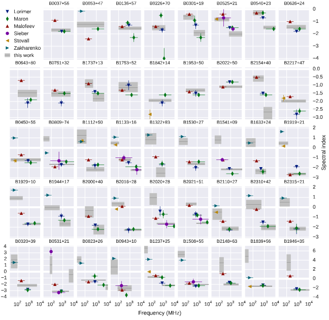
Figure 9: Comparison of spectral indices from this work (grey-shaded rectangles) to the ones reported by Sieber (1973), Lorimer et al. (1995), Maron et al. (2000), Malofeev et al. (2000), Zakharenko et al. (2013), and Stovall et al. (2015) (coloured points with error bars). The horizontal extent of grey rectangles and horizontal error bars on literature values represent the frequency range over which the index was measured. The vertical extent/error bar marks the reported uncertainty (for Malofeev et al. 2000 and Zakharenko et al. 2013 no errors were given). Spectral fits in this work include data points from all these works together with other published values and our own measurements. The pulsars are grouped by the spectral index plotting limits and ordered by right ascension within each group.

For the negative spectral indices, the $\alpha$ at frequencies above the break is generally steeper than at frequencies below the break, with the exception of PSRs B0531$+$21, B0114$+$58, and B2303$+$30, for which the spectra flatten at higher frequencies. It must be noted that for the latter two sources the flattening is based on a single flux density measurement and more data are needed to confirm the observed behaviour. In case of the Crab pulsar, the flux density measurements at 5 and 8 GHz (Moffett & Hankins, 1996) suggest that spectral index may flatten somewhere between 2 and 5 GHz. Such flattening coincides with a dramatic profile transformation happening in the same frequency range (Hankins et al., 2015) and is also suggested by spectral index measurements for the individual profile components (Moffett & Hankins, 1999).

Figure 7 shows the spectral indices below and above the break frequency for the 32 census pulsars with a relatively well-known spectra with $\nu_{\mathrm{min}}<200$ MHz and $\nu_{\mathrm{max}}>4$ GHz, consisting of at least 10 flux density measurements. The data confirm a previously noticed tendency (Sieber, 1973): in most cases, if the break happens at rather higher frequencies ($\nu_{\mathrm{br}}\gtrsim 500$ MHz), the change in slope is relatively moderate, with $\alpha_{\mathrm{lo}}-\alpha_{\mathrm{hi}}\approx 1$ or 2 (the so-called “high-frequency cut-off”). For the breaks at lower frequencies ($\nu_{\mathrm{br}}\lesssim 300$ MHz), the change is more dramatic, with low-frequency $\alpha$ close to or larger than nought, the so-called “low-frequency turnover”. Possible statistical relationships between the turnover frequency, cut-off frequency and pulsar period had been previously investigated in several works (e.g. Malofeev & Malov, 1980; Izvekova et al., 1981), and a number of theoretical explanations was proposed (Malofeev & Malov, 1980; Ochelkov & Usov, 1984; Malov & Malofeev, 1991; Petrova, 2002; Kontorovich & Flanchik, 2013).

Because of the typically large spread of the same-frequency $S_{\nu}$ measurements, the reliable identification of the break frequencies is feasible only for the well-known spectra, composed of multiple, densely spaced flux density measurements, obtained in a wide frequency range. The census data alone appears to be insufficient for making a substantial contribution to the spectral break identification. The HBA band appears to be situated close to or within the frequency range where a spectral turnover is likely to happen for the majority of non-recycled pulsars (at least in the census sample), and, apart from a few dozens of the previously well-studied sources, the literature spectra of census pulsars were scarcely sampled or did not extend below the HBA band (i.e. below 100 MHz). The studies of low-frequency turnover would considerably benefit from the future flux density measurements at frequencies $<100$ MHz, which could be obtained with the currently operating LWA, UTR-2, LOFAR LBA, and the future standalone NenuFAR LOFAR Super Station in Nançay (Zarka et al., 2012).

The census data still provide an indirect indication of the low-frequency turnover in some relatively poorly sampled spectra. This evidence comes from the comparison of the spectral indices for pulsars best fitted with 1PL in the work of Maron et al. (2000) and in our work. The census sample contains 35 such pulsars, with the indices mostly based on the data from 100 MHz–5 GHz. The corresponding indices from Maron et al. (2000) are based on flux measurements between 400 MHz and 1.6/5 GHz. There is a statistical preference for a spectral index to be flatter in our broader frequency range (Fig. 8), which could indicate a turnover happening somewhere close to 100 MHz. As a comparison, we plot the spectral indices for 21 pulsars with clearly identified low-frequency turnover happening below the frequency range of Maron et al. (2000). Such pulsars generally exhibit better spectral index agreement.

5.4.4 Comparison to the indices from the literature

For some of the census pulsars several spectral index estimates have already been made by various authors. Our spectra generally include the flux densities reported in those works, together with the other published flux densities and our own measurements. Thus, it is interesting to compare our spectral indices to the ones available from the literature. Such a comparison can serve as an estimate of how much the spectral index values could change with addition of new data points in the same frequency range or with expansion of the frequency coverage.

We have compiled the spectral index measurements from several works with single or broken PL fits, namely from Sieber (1973); Lorimer et al. (1995); Maron et al. (2000), and Malofeev et al. (2000). A recent set of spectral index measurements for frequencies below 100 MHz from Zakharenko et al. (2013) and Stovall et al. (2015) were added as well. The collection of spectral indices versus the respective frequency ranges for the pulsars with at least three such literature measurements is shown in Fig. 9.

Two features can be gleaned from this plot. Firstly, even if all authors approximate the spectrum with a single PL in the frequency range available to them, sometimes the spectral indices in more narrow frequency sub-ranges may differ from each other and from the spectral index in a broader frequency range. This spread can reach a magnitude of $\delta\alpha$ of about 0.5 or even 1.5 (e.g. for PSRs B0053$+$47, B1929$+$21, and others). This can be explained by a systematic error in individual flux density measurements that bias the spectral index estimate, if the number of data points is small or the frequency range is narrow.

Secondly, different authors do not always agree on the location of the spectral breaks (e.g. for PSRs B0136$+$57, B2020$+$51, and others). Sometimes the narrowband spectral index shows clear gradual evolution with frequency across the radio band (e.g. for PSRs B1133$+$16 and B1237$+$25). To a certain degree, this gradual evolution can be influenced by the scatter of flux density measurements, which “smooths” the breaks. However, one can also question whether a collection of PLs is a good representation of broadband spectral shape in general.

More complex models of broadband pulsar spectra (usually including a PL and absorption components) have been proposed by several authors (e.g. Sieber 1973; Malofeev & Malov 1980 for the low-frequency turnover, and Lewandowski et al. 2015; Rajwade et al. 2016 for the gigahertz-peaked spectra). However, in general, progress has been impeded by the lack of accepted emission theories and the poor sampling of the available spectra. The empirical parabola fit in $\log\nu$–$\log S$ space was proposed by Kuzmin & Losovsky (2001) and subsequently used for approximating the gigahertz-peaked spectra (e.g. Dembska et al., 2014). Recently, a simple three-parameter functional form for pulsar spectra was suggested by Löhmer et al. (2008). This form is based on a flicker noise model, which assumes the observed pulsar emission to be a collection of separate nanosecond-scale shots. However, the flicker noise model predicts flattening of the spectrum at lower frequencies ($\alpha\approx 0$), not the turnover ($\alpha>0$), and thus requires more development.

6 Summary

We have observed 194 non-recycled northern pulsars with the LOFAR high-band antennas in the frequency range of 110–188 MHz. This is a complete (as of September 2013) census of known non-recycled radio pulsars at $\mathrm{Dec}>8\degree$ and $|\mathrm{Gb}|>3\degree$, excluding globular cluster pulsars and those with poorly defined positions. Each pulsar was observed contiguously for 20 min or at least 1000 spin periods.

We have detected 158 pulsars, collecting one of the largest samples of low-frequency wide-band data. These observations provided a wealth of information for the ongoing investigation of the low-frequency properties of pulsar radio emission, including the time-averaged and single-pulse full-Stokes analyses. Precise measurements of the ISM parameters (such as DM, RM, and scattering) along many lines of sight are being obtained as well.

In this work we present the DMs, flux densities and flux-calibrated profiles for 158 detected pulsars. The average profiles, DM and flux density measurements will be made publicly available via the EPN Database of Pulsar Profiles and on a dedicated LOFAR web-page. The LBA (30–90 MHz) extension of the census has also been observed and its results will be presented in subsequent works.

Owing to the large fractional bandwidth, we were able to measure DMs with typically ten times better precision than in the pulsar catalogue (with the median error of census DMs equal to $1.5\times 10^{-3}$ pc cm^-3). For our DM measurements we assumed the absence of profile evolution across the HBA band. The value of DM could change by an amount that is an order of magnitude larger than the measurement error under different profile evolution assumptions. We computed the rate of secular DM variations by comparing census and catalogue DMs. The spread of the rates was similar to that found by Hobbs et al. (2004b), however, we also find an excess of larger DM variation rates for the pulsars with larger reported DM errors, possibly indicating that some DM errors were unaccounted for. We also compared our DMs to similar recent measurements at $\nu<100$ MHz and found generally more preference for the larger DM variation rates, which may be due to the relative influence of shorter-timescale stochastic variation in the ISM, but also may be caused by offsets in DM introduced by profile evolution and scattering.

For two of the detected pulsars the ISM properties differ from what was expected. PSR J1503+2111 was detected at a DM of 3.260 pc cm^-3, in contrast to the pulsar catalogue value of 11.75 pc cm^-3 (Champion et al., 2005a). We suggest that the catalogue value may be incorrect. Another pulsar, PSR B2036$+$53, appeared to have a scattering time three orders of magnitude smaller than predicted by the NE2001 model.

PSR J1740+1000, previously considered to have a gigahertz-peaked spectrum, was detected at the LOFAR HBA frequencies with 20 times larger flux density than predicted by the fits in Dembska et al. (2014) and Rajwade et al. (2016). We argue that this pulsar has a normal power-law spectrum with an unusually large amount of flux density variability.

We have constructed spectra for census pulsars by combining our measurements with those from the literature. Spectra were fitted with a single or a broken PL (with one or two breaks). Out of 165 spectra (some spectra consisted only of the literature points when the pulsars were not detected in the census), 124 were best fitted using a single PL, although those were also spectra with the smallest number of flux density measurements. We also include spectral fits for 48 pulsars that do not have a previously published value. The distribution of spectral indices for these pulsars agrees with that found in a similar frequency range by Malofeev et al. (2000) and is generally flatter ($\bar{\alpha}=-1.4$) than the distribution at higher frequencies ($\bar{\alpha}=-1.8$, Maron et al., 2000).

The census data alone appear to be insufficient for making a considerable contribution to low-frequency turnover studies, since the HBA frequency range is located close to or within the frequency range where spectral turnover is likely to happen for the majority of non-recycled pulsars (at least for the census sample). Since the lower-frequency data (below 100 MHz) are normally absent or scarce, for many sources the turnover can be observed only as a slight flattening of the spectrum at the low-frequency edge. Studies of the low-frequency turnover will considerably benefit from future flux measurements below 100 MHz.

For a sub-sample of pulsars with relatively well-measured spectra, we have compared the obtained broadband spectral indices to the ones reported in the literature. It appears that sometimes spectral indices in more narrow sub-ranges may differ considerably ($\delta\alpha$ of $\approx 0.5-1.5$) from each other and from the spectral index in a broader frequency range. This can be explained by errors that are unaccounted for in individual flux density measurements, which bias the spectral index estimate if the number of data points is small or the frequency range is narrow. Also, different authors do not always agree on the location of the spectral breaks and sometimes the narrowband spectral index shows clear gradual evolution with frequency across the radio band. To some degree this gradual evolution can be influenced by the scatter of flux density measurements. However, this may also be an indication that a collection of PLs is not a good representation of the broadband spectral shape of pulsar radio emission.

Appendix A Scintillation

Inhomogeneities in the ISM introduce phase modulations to the propagating pulsar radio emission and cause the observed flux density to fluctuate both in time and radio frequency. To estimate the influence of scintillation on census flux densities, we used predictions of a simple thin-screen Kolmogorov model, summarised in Lorimer & Kramer (2005). The scintillation bandwidth was determined as $\Delta f=1.16/(2\pi\tau_{\mathrm{scat}})\times($150 MHz/1 GHz$)^{4.4}$, where $\tau_{\mathrm{scat}}$ is scattering time at 1 GHz from the NE2001 model (Cordes & Lazio 2002). For PSR B2036+53 we changed the obviously incorrect NE2001 prediction, $\tau_{\mathrm{scat}}($150 MHz$)=486$ s, to a more reasonable $\tau_{\mathrm{scat}}($150 MHz$)\approx 200$ ms, estimated from the census data at the lower edge of HBA band (note that Table LABEL:table:main lists NE2001 value of $\tau_{\mathrm{scat}}$ for this pulsar, for consistency with other sources).

For all census pulsars the scintillation bandwidth $\Delta f$ was of the order of 0.1 kHz$-$1 MHz, indicating that the strong scintillation regime dominates ($\sqrt{f/\Delta f}>1$). To calculate the diffractive scintillation (DISS) time scales, we used distances and transverse velocities from the pulsar catalogue. The velocities were taken to be 200 km s^-1 if no direct measurements were available. DISS time scales ranged from a few seconds to a few minutes. Thus, for all pulsars band- and session-integrated flux density measurements were averaged over many scintles both in the time and frequency domain, and thus were not expected to be influenced by DISS: the modulation index $m_{\mathrm{DISS}}$ (rms of the flux density divided by its mean value) was $\approx 0.001$. The refractive scintillation (RISS), however, was much more prominent, with typical $m_{\mathrm{RISS}}\approx 0.1$. The expected values of total modulation index are given in Table LABEL:table:main.

Appendix B Tables

Table LABEL:table:main contains observation summary. The columns indicate: pulsar name; spin period; observing epoch; observation length; peak S/N of the average profile; DM from the pulsar catalogue; measured census DM; expected NE2001 scattering time at 150 MHz divided by pulsar period; expected modulation index due to scintillation in the ISM; mean flux density within the HBA band (upper limit for the non-detected pulsars), and the literature references to previous flux density measurements. The values in brackets indicate the errors on the last one or two significant digits.

Tables LABEL:table:1pl–LABEL:table:3pl contain fitted parameters for the pulsars with the spectra modelled with a single PL, a PL with one break and a PL with two breaks, respectively. The columns include pulsar name; spectral frequency span; number of data points in spectrum, $N_{p}$; the reference frequency, $\nu_{0}$; flux density at the reference frequency, $S_{0}$; spectral index, $\alpha$ (or indices in case of broken PLs), and fitted flux density scatter, $\sigma^{\mathrm{unkn}}_{\lg S}$ (if applicable, see Sect. 5.2). Tables LABEL:table:2pl and LABEL:table:3pl also include break frequency, $\nu_{\mathrm{br}}$, together with its 68% uncertainty range.

Table 3: Observation summary, DM and flux density measurements.

PSR	Period $P$ (s)	Observing epoch (MJD)	Obs. time (min)	Peak S/N	$\mathrm{DM}_{\mathrm{cat}}$ (pc cm-3)	$\mathrm{DM_{\mathrm{cen}}}$ (pc cm-3)	Expec- ted $\tau_{\mathrm{scat}}/P$	Exp. mod. index	Mean HBA flux (mJy)	Literature flux references
J0006+1834	0.694	56703.58	20	0006	12.0 (6)	11.41 (55)	4e-05	0.20	6.5 $\pm$ 3.3	8, 52, 71
B0011+47	1.241	56773.46	21	0036	30.85 (7)	30.405 (13)	2e-04	0.13	35 $\pm$ 18	17, 20, 24, 41, 45, 49, 61
J0033+57	0.315	56773.48	20	0$\dots$	76	$\dots$	2e-02	0.08	00000¡2.0	…
B0037+56	1.118	56753.42	20	0038	92.595 (9)	92.5146 (25)	1e-02	0.07	33 $\pm$ 17	18, 28, 41, 52, 61
B0045+33	1.217	56703.61	21	0098	39.94 (4)	39.922 (15)	5e-04	0.11	13 $\pm$ 6	18, 41, 49, 52, 61, 68
B0052+51	2.115	56776.32	36	0035	44.125 (15)	44.0127 (24)	4e-04	0.11	9.4 $\pm$ 4.7	18, 20, 41, 49, 52
B0053+47	0.472	56703.59	20	0019	18.09 (4)	18.1354 (13)	2e-04	0.16	7.5 $\pm$ 3.8	18, 28, 41, 52, 68, 71
B0105+65	1.284	56784.40	22	0088	30.46 (5)	30.5482 (14)	3e-04	0.12	41 $\pm$ 20	14, 24, 41, 45, 52, 53, 61
B0105+68	1.071	56703.62	20	0029	61.092 (16)	61.0617 (36)	2e-03	0.09	8.9 $\pm$ 4.5	18, 41, 52, 61, 68
J0106+4855	0.083	56780.46	20	0$\dots$	70.9 (2)	$\dots$	3e-02	0.09	00000¡1.6	55
B0114+58	0.101	56780.47	20	0088	49.423 (4)	49.42068 (59)	2e-02	0.10	79 $\pm$ 39	20, 38, 41, 52, 64
B0136+57	0.272	56753.45	20	0394	73.779 (6)	73.81141 (76)	4e-02	0.07	250 $\pm$ 130	17, 24, 41, 49, 52, 60, 61
J0137+1654	0.415	56703.64	20	0018	26.6 (4)	26.0838 (24)	6e-04	0.13	6.2 $\pm$ 3.1	40, 71
J0152+0948	2.747	56784.43	46	0012	21.87 (2)	22.881 (12)	7e-05	0.14	1.7 $\pm$ 1.1	6, 71
B0153+39	1.812	56773.50	31	0020	60.0 (6)	59.833 (11)	9e-04	0.10	8.5 $\pm$ 4.3	18, 20, 41, 52, 68
J0205+6449	0.066	56784.39	20	0$\dots$	140.7 (3)	$\dots$	9e-01	0.05	00000¡2.2	11
J0212+5222	0.376	56773.52	20	0023	38	38.23555 (45)	2e-03	0.11	12 $\pm$ 6	2
B0226+70	1.467	56703.68	25	0021	46.64 (3)	46.6794 (16)	7e-04	0.10	5.3 $\pm$ 2.7	18, 41, 45, 49, 52, 61, 68
B0301+19	1.388	56703.69	24	0146	15.737 (9)	15.65677 (35)	9e-05	0.15	42 $\pm$ 21	19, 23, 24, 28, 41, 45, 49, 50, 51, 52, 60, 61, 63, 71
B0320+39	3.032	56703.72	51	0625	26.01 (3)	26.18975 (93)	1e-04	0.12	92 $\pm$ 46	17, 19, 24, 28, 30, 41, 45, 49, 61, 63, 71
J0324+5239	0.337	56780.49	20	0009	119	115.4636 (29)	1e-01	0.06	5.9 $\pm$ 3.0	2
J0329+1654	0.893	56703.74	20	0006	42.1 (2)	40.821 (36)	8e-04	0.11	2.3 $\pm$ 1.3	40
B0331+45	0.269	56747.65	20	0143	47.153 (3)	47.14571 (29)	4e-03	0.10	34 $\pm$ 17	18, 41, 45, 52, 61
B0402+61	0.595	56747.67	20	0048	65.303 (7)	65.4053 (34)	6e-03	0.08	29 $\pm$ 15	17, 41, 49, 52, 53, 61
B0410+69	0.391	56773.55	20	0077	27.465 (4)	27.44598 (38)	8e-04	0.13	28 $\pm$ 14	18, 20, 28, 41, 52, 61, 71
J0413+58	0.687	56773.54	20	0$\dots$	57	$\dots$	3e-03	0.09	00000¡1.9	…
J0417+35	0.654	56773.56	20	0031	51 (10)	48.5336 (12)	2e-03	0.10	9.0 $\pm$ 4.5	9, 52
J0419+44	1.241	56772.59	21	0$\dots$	71	$\dots$	4e-03	0.08	00000¡1.9	…
J0435+27	0.326	56773.58	20	0020	53 (5)	53.18193 (24)	4e-03	0.10	7.0 $\pm$ 3.5	52, 58
B0450+55	0.341	56772.61	20	0275	14.495 (7)	14.59002 (15)	3e-04	0.15	91 $\pm$ 46	41, 49, 52, 53, 61, 63, 65, 71
B0458+46	0.639	56779.56	20	0009	42.187 (8)	41.834 (20)	2e-03	0.10	17 $\pm$ 8	17, 24, 41, 49, 52, 61
B0523+11	0.354	56703.77	20	0032	79.345 (3)	79.418 (13)	1e-02	0.08	34 $\pm$ 17	19, 24, 41, 45, 50, 52, 53, 61
B0525+21	3.746	56747.71	63	0746	50.937 (17)	50.8695 (13)	3e-04	0.10	230 $\pm$ 120	5, 12, 23, 24, 41, 45, 47, 49, 51, 52, 61, 63, 66
B0531+21	0.033	56703.78	20	0120	56.791 (1)	56.77118 (24)	2e-01	0.08	7500 $\pm$ 3800	1, 28, 41, 43, 45, 48, 51, 52, 53, 57, 61
B0540+23	0.246	56779.57	20	0039	77.7115 (17)	77.7026 (10)	5e-02	0.07	36 $\pm$ 18	14, 19, 23, 24, 30, 34, 41, 47, 49, 51, 52, 53, 56, 61
B0609+37	0.298	56772.66	20	0050	27.135 (4)	27.15495 (34)	1e-03	0.12	21 $\pm$ 10	28, 41, 49, 52, 61, 64, 71
J0611+30	1.412	56772.64	24	0078	73 (5)	45.2551 (16)	8e-04	0.10	45 $\pm$ 23	9
B0626+24	0.477	56747.76	20	0160	84.195 (4)	84.1762 (50)	3e-02	0.07	73 $\pm$ 36	17, 19, 28, 41, 49, 52, 53, 61
B0643+80	1.214	56747.78	21	0097	33.332 (17)	33.31882 (71)	4e-04	0.12	19 $\pm$ 9	28, 41, 45, 52, 61
J0646+0905	0.904	56779.67	20	0$\dots$	149.0 (7)	$\dots$	7e-02	0.05	00000¡3.1	3
J0647+0913	1.235	56779.59	21	0$\dots$	154.7 (12)	$\dots$	5e-02	0.05	00000¡3.3	3
B0655+64	0.196	56772.68	20	0112	8.771 (5)	8.77387 (27)	9e-05	0.22	51 $\pm$ 25	17, 41, 44, 61, 63, 65, 71
B0656+14	0.385	56747.75	20	0015	13.977 (13)	14.0762 (24)	3e-04	0.15	11 $\pm$ 5	24, 41, 49, 50, 52, 61, 69, 71
J0711+0931	1.214	56779.74	21	0006	45.0 (1)	46.238 (13)	8e-04	0.11	3.1 $\pm$ 1.8	42
B0751+32	1.442	56772.72	25	0104	39.949 (8)	39.9863 (14)	5e-04	0.11	17 $\pm$ 9	17, 24, 28, 41, 52, 61
B0809+74	1.292	56747.80	22	0661	5.733 (1)	5.75066 (48)	9e-06	0.23	300 $\pm$ 150	5, 15, 23, 24, 28, 30, 32, 35, 41, 45, 47, 49, 51, 52, 53, 61, 65, 71
J0815+0939	0.645	56781.71	20	0007	52.667 (9)	52.6589 (79)	2e-03	0.10	6.8 $\pm$ 3.5	6
B0823+26	0.531	56747.82	20	1589	19.454 (4)	19.47633 (18)	2e-04	0.15	520 $\pm$ 260	5, 12, 16, 23, 24, 30, 34, 38, 40, 41, 45, 47, 49, 51, 52, 53, 61, 63, 65, 70, 71
B0841+80	1.602	56747.83	27	0023	34.66 (17)	34.8121 (31)	3e-04	0.12	5.9 $\pm$ 3.0	18, 20, 52, 61, 68
B0917+63	1.568	56747.89	27	0164	13.158 (18)	13.15423 (18)	4e-05	0.17	22 $\pm$ 11	18, 20, 41, 52, 68, 71
B0940+16	1.087	56687.10	20	0021	20.32 (5)	20.3402 (18)	1e-04	0.14	26 $\pm$ 13	19, 24, 40, 41, 50, 61, 69, 71
B0943+10	1.098	56779.82	20	0882	15.4 (5)	15.31845 (90)	7e-05	0.16	440 $\pm$ 220	15, 24, 41, 45, 51, 52, 53, 56, 61, 65, 71
J0943+22	0.533	56747.86	20	0033	25.1 (6)	27.2676 (16)	5e-04	0.13	6.3 $\pm$ 3.2	52, 67
J0947+27	0.851	56747.88	20	0024	29 (3)	28.886 (26)	4e-04	0.13	10 $\pm$ 5	58, 71
B1112+50	1.656	56747.93	28	0500	9.195 (8)	9.18634 (26)	3e-05	0.17	50 $\pm$ 25	23, 24, 33, 41, 45, 47, 49, 51, 52, 53, 61, 63, 71
B1133+16	1.188	56687.11	20	2220	4.8451 (1)	4.84066 (34)	3e-05	0.19	940 $\pm$ 470	5, 12, 15, 16, 23, 24, 30, 32, 31, 33, 34, 35, 38, 41, 45, 47, 49, 50, 51, 52, 53, 61, 63, 65, 66, 70, 71
B1237+25	1.382	56689.15	24	0854	9.242 (6)	9.25159 (53)	2e-05	0.20	170 $\pm$ 90	5, 12, 19, 23, 24, 30, 32, 41, 45, 47, 49, 51, 52, 53, 61, 63, 65, 66, 71
J1238+21	1.119	56687.14	20	0133	17.5 (12)	17.9706 (31)	1e-04	0.15	27 $\pm$ 13	52, 58, 71
J1246+22	0.474	56747.99	20	0021	17.9 (1)	17.7978 (18)	3e-04	0.15	4.2 $\pm$ 2.1	52, 67, 71
J1313+0931	0.849	56779.92	20	0152	12.0 (1)	12.040623 (43)	7e-05	0.17	48 $\pm$ 24	42, 71
B1322+83	0.670	56687.19	20	0090	13.312 (18)	13.31624 (76)	6e-05	0.18	28 $\pm$ 14	20, 28, 41, 45, 52, 53, 68, 71
J1503+2111	3.314	56687.22	56	0043	11.75 (6)	3.2603 (41)	4e-08	0.62	4.6 $\pm$ 2.4	6, 20, 71
B1508+55	0.740	56687.26	20	3384	19.61 (2)	19.6189 (13)	6e-04	0.12	770 $\pm$ 390	23, 24, 30, 32, 35, 41, 45, 47, 49, 51, 52, 60, 61, 63, 65, 71
B1530+27	1.125	56703.26	20	0072	14.698 (18)	14.691 (16)	2e-05	0.20	33 $\pm$ 17	17, 40, 41, 44, 45, 49, 52, 61, 71
B1541+09	0.748	56780.02	20	0544	35.24 (3)	34.9758 (16)	3e-03	0.09	770 $\pm$ 380	23, 24, 28, 41, 45, 47, 49, 50, 51, 52, 53, 60, 61, 63, 65
J1549+2113	1.262	56703.27	22	0031	24.8 (2)	24.0553 (36)	2e-04	0.13	7.2 $\pm$ 3.7	20, 40, 52, 71
J1612+2008	0.427	56687.25	20	0015	19.544 (1)	19.5082 (32)	4e-04	0.14	7.0 $\pm$ 3.6	4
J1627+1419	0.491	56687.29	20	0064	33.8 (6)	32.16696 (84)	1e-03	0.12	78 $\pm$ 39	20, 39, 52
B1633+24	0.491	56748.14	20	0135	24.32 (4)	24.2671 (44)	6e-04	0.13	79 $\pm$ 40	41, 52, 53, 61, 68, 69, 71
J1645+1012	0.411	56687.33	20	0087	36.3 (6)	36.17129 (19)	2e-03	0.11	69 $\pm$ 35	39, 52
J1649+2533	1.015	56748.12	20	0025	35.5 (9)	34.4622 (78)	6e-04	0.11	12 $\pm$ 6	20, 39, 52
J1652+2651	0.916	56748.11	20	0033	40.8 (2)	40.80244 (17)	1e-03	0.11	20 $\pm$ 10	20, 39, 40, 52, 62
J1720+2150	1.616	56748.15	27	0016	41.1 (4)	40.719 (35)	5e-04	0.11	4.5 $\pm$ 2.3	20, 39, 52
B1737+13	0.803	56687.30	20	0161	48.673 (4)	48.66823 (43)	5e-04	0.12	81 $\pm$ 40	28, 41, 49, 50, 52, 53, 60, 61
J1740+1000	0.154	56687.37	20	0006	23.85 (5)	23.897 (25)	1e-03	0.14	9.4 $\pm$ 4.8	13, 29, 46, 71
J1741+2758	1.361	56773.14	23	0093	29.3 (6)	29.14487 (11)	2e-04	0.13	30 $\pm$ 15	20, 39, 52, 71
J1746+2245	3.465	56784.14	58	0025	52 (2)	49.8543 (57)	3e-04	0.10	4.5 $\pm$ 2.3	6, 20
J1746+2540	1.058	56784.17	20	0013	51.5 (2)	51.2044 (33)	1e-03	0.10	3.7 $\pm$ 2.0	20, 39
J1752+2359	0.409	56783.18	20	0020	36.0 (9)	36.19635 (60)	1e-03	0.12	5.3 $\pm$ 2.8	39, 52
B1753+52	2.391	56785.18	40	0017	35.35 (1)	35.0096 (64)	2e-04	0.12	2.4 $\pm$ 1.3	18, 20, 28, 41, 52
J1758+3030	0.947	56784.19	20	0157	34.9 (1)	35.0674 (14)	4e-04	0.12	56 $\pm$ 28	9, 20, 52, 62
J1806+1023	0.484	56687.38	20	0$\dots$	52.03 (7)	$\dots$	2e-03	0.10	00000¡3.2	…
B1811+40	0.931	56780.05	20	0103	41.487 (18)	41.55656 (22)	7e-04	0.11	50 $\pm$ 25	13, 17, 24, 28, 41, 44, 53, 61
J1813+1822	0.336	56748.17	20	0$\dots$	60.8 (5)	$\dots$	5e-03	0.10	00000¡2.5	39
J1814+1130	0.751	56687.40	20	0$\dots$	65 (1)	$\dots$	3e-03	0.09	00000¡3.3	54
J1819+1305	1.060	56687.31	20	0013	64.9 (4)	64.808 (13)	2e-03	0.09	13 $\pm$ 7	20, 54
J1821+1715	1.367	56703.30	23	0025	60.47 (7)	60.2844 (25)	1e-03	0.10	11 $\pm$ 5	6, 20, 58
J1822+1120	1.787	56687.35	30	0$\dots$	95.2 (6)	$\dots$	3e-03	0.08	00000¡3.1	40
J1828+1359	0.742	56703.33	20	0$\dots$	56 (1)	$\dots$	2e-03	0.10	00000¡3.2	20, 54
J1834+10	1.173	56748.18	20	0005	62 (12)	78.479 (24)	3e-03	0.09	5.2 $\pm$ 2.9	9, 52
J1837+1221	1.964	56687.48	33	0$\dots$	100.6 (4)	$\dots$	3e-03	0.08	00000¡3.6	…
J1838+1650	1.902	56801.09	32	0084	33.9 (2)	32.95162 (99)	1e-04	0.13	26 $\pm$ 13	20, 40
B1839+09	0.381	56783.19	20	0110	49.107 (8)	49.1579 (43)	2e-03	0.11	130 $\pm$ 70	28, 41, 44, 49, 50, 53, 61
B1839+56	1.653	56789.09	28	0532	26.698 (11)	26.77163 (17)	3e-04	0.12	76 $\pm$ 38	24, 35, 41, 45, 49, 52, 53, 61, 63, 65, 71
J1842+1332	0.472	56703.36	20	0$\dots$	102.5 (7)	$\dots$	1e-02	0.08	00000¡3.4	…
B1842+14	0.375	56703.31	20	0145	41.51 (4)	41.48555 (61)	1e-03	0.11	110 $\pm$ 50	24, 41, 45, 49, 50, 53, 59, 61, 63
J1843+2024	3.407	56785.21	57	0$\dots$	85.3 (2)	$\dots$	1e-03	0.08	00000¡2.0	6
J1848+0826	0.329	56780.06	20	0003	90.77 (7)	90.677 (80)	2e-02	0.08	6.5 $\pm$ 4.2	8, 21
B1848+12	1.205	56687.43	21	0053	70.615 (16)	70.6333 (17)	2e-03	0.09	37 $\pm$ 19	21, 28, 41, 52, 64
B1848+13	0.346	56703.34	20	0010	60.147 (8)	60.1396 (66)	4e-03	0.10	5.7 $\pm$ 3.1	21, 41, 49, 52, 64
J1849+2423	0.276	56788.06	20	0009	62.239 (5)	62.2677 (16)	5e-03	0.10	8.1 $\pm$ 4.1	6, 20
B1852+10	0.573	56687.42	20	0$\dots$	207.2 (3)	$\dots$	6e-02	0.06	00000¡5.4	21, 64
J1853+0853	3.915	56784.22	66	0$\dots$	214 (5)	$\dots$	2e-02	0.05	00000¡4.3	37
J1859+1526	0.934	56773.18	20	0008	97.45 (2)	97.45 (1)	5e-03	0.08	6.7 $\pm$ 3.7	8, 20
J1900+30	0.602	56776.26	20	0014	65 (13)	71.8352 (22)	3e-03	0.09	5.9 $\pm$ 3.0	9
J1901+1306	1.831	56788.14	31	0012	75.03 (8)	75.0988 (60)	1e-03	0.09	6.5 $\pm$ 3.5	8
J1903+2225	0.651	56788.08	20	0$\dots$	109.2 (3)	$\dots$	9e-03	0.08	00000¡2.8	8, 20
B1905+39	1.236	56789.13	21	0119	30.96 (3)	30.966 (14)	3e-04	0.13	46 $\pm$ 23	17, 24, 28, 41, 49, 61
J1906+1854	1.019	56773.19	20	0017	156.72 (4)	156.7676 (30)	1e-02	0.07	18 $\pm$ 9	8, 20
J1908+2351	0.378	56779.26	20	0004	101.5 (7)	101.695 (15)	1e-02	0.08	2.3 $\pm$ 1.5	39
J1909+1859	0.542	56748.20	20	0013	64.477 (7)	64.517 (26)	3e-03	0.10	6.0 $\pm$ 3.1	8, 20
B1910+20	2.233	56788.11	38	0017	88.34 (3)	88.5961 (62)	2e-03	0.08	3.5 $\pm$ 1.9	14, 41, 44, 56, 59, 61
J1911+1758	0.460	56781.25	20	0009	48.971 (13)	48.98 (16)	1e-03	0.12	8.0 $\pm$ 4.2	8, 20
J1912+2525	0.622	56788.23	20	0042	37.836 (8)	37.8474 (16)	3e-04	0.14	18 $\pm$ 9	8, 20
J1913+3732	0.851	56801.13	20	0015	69	72.3263 (41)	2e-03	0.09	7.1 $\pm$ 3.6	2
B1915+22	0.426	56801.11	20	0014	134.93 (12)	134.7495 (34)	2e-02	0.07	12 $\pm$ 6	64
B1918+26	0.786	56748.21	20	0095	27.62 (9)	27.70882 (82)	1e-04	0.16	21 $\pm$ 10	18, 20, 40, 41, 49, 52, 68, 71
B1919+21	1.337	56788.21	23	2054	12.4370 (1)	12.44399 (63)	3e-05	0.18	1300 $\pm$ 700	14, 15, 19, 23, 24, 32, 35, 41, 45, 47, 49, 51, 52, 59, 61, 63, 65, 71
J1927+0911	0.290	56788.16	20	0$\dots$	202.7 (4)	$\dots$	1e-01	0.06	00000¡5.2	37
B1929+10	0.227	56781.21	20	0314	3.18 (4)	3.18321 (16)	3e-05	0.25	540 $\pm$ 270	5, 12, 14, 16, 20, 21, 24, 27, 30, 34, 38, 40, 41, 45, 47, 49, 50, 51, 52, 53, 59, 61, 66, 71
B1930+13	0.928	56781.26	20	0005	177.9 (2)	177.01 (15)	3e-02	0.06	4.9 $\pm$ 3.0	20, 21, 22, 36, 53, 68
J1937+2950	1.657	56776.27	28	0006	113.8 (2)	113.99 (11)	4e-03	0.08	12 $\pm$ 6	25
J1941+1026	0.905	56687.45	20	0$\dots$	138.91 (2)	$\dots$	1e-02	0.07	00000¡3.2	8, 20
J1941+1341	0.559	56687.50	20	0$\dots$	147.9 (3)	$\dots$	2e-02	0.07	00000¡3.6	37
B1942+17	1.997	56788.18	34	0$\dots$	175 (2)	$\dots$	1e-02	0.06	00000¡2.5	20, 22, 24, 36, 53, 61, 68
B1944+17	0.441	56801.14	20	0029	16.22 (16)	16.1356 (73)	4e-04	0.14	41 $\pm$ 20	14, 24, 41, 47, 49, 50, 53, 59, 60, 61, 71
B1946+35	0.717	56748.23	20	0028	129.075 (3)	129.36748 (78)	6e-02	0.06	170 $\pm$ 90	14, 19, 41, 45, 47, 49, 52, 56, 59, 61
J1947+0915	1.481	56779.27	25	0$\dots$	94 (4)	$\dots$	3e-03	0.08	00000¡3.8	…
B1949+14	0.275	56703.44	20	0013	31.46 (9)	31.5051 (47)	5e-04	0.15	6.4 $\pm$ 3.3	20, 64
J1951+1123	5.094	56703.40	85	0007	31.29 (9)	26.8 (33)	2e-05	0.16	8.2 $\pm$ 4.1	8, 20, 40
J1953+1149	0.852	56687.46	20	0$\dots$	140.03 (3)	$\dots$	1e-02	0.07	00000¡2.9	8, 40
B1953+50	0.519	56789.06	20	0155	31.974 (3)	31.98266 (13)	3e-04	0.14	48 $\pm$ 24	17, 24, 41, 44, 49, 52, 61
J1956+0838	0.304	56781.27	20	0006	68.2 (13)	67.087 (24)	6e-03	0.09	9.2 $\pm$ 4.8	…
J1959+3620	0.406	56789.18	20	0$\dots$	273	$\dots$	2e-01	0.05	00000¡3.5	2
B2000+40	0.905	56776.29	20	0008	131.334 (12)	131.486 (41)	9e-03	0.07	29 $\pm$ 15	28, 41, 52, 61, 64
J2002+1637	0.276	56773.22	20	0004	94.39 (8)	94.581 (48)	1e-02	0.08	1.8 $\pm$ 1.2	8, 40
J2007+0809	0.326	56779.29	20	0010	53.9 (10)	53.394 (37)	3e-03	0.10	32 $\pm$ 16	…
J2007+0910	0.459	56784.25	20	0036	48.6 (2)	48.72934 (67)	2e-03	0.11	26 $\pm$ 13	6
J2008+2513	0.589	56753.34	20	0010	60.554 (9)	60.5555 (36)	1e-03	0.11	3.8 $\pm$ 2.1	8, 20, 52
J2015+2524	2.303	56788.25	39	0$\dots$	13 (3)	$\dots$	8e-06	0.21	00000¡2.0	8, 71
B2016+28	0.558	56781.23	20	1255	14.172 (4)	14.1839 (13)	3e-04	0.14	810 $\pm$ 410	5, 12, 14, 23, 24, 28, 30, 41, 47, 49, 51, 52, 53, 59, 60, 61, 63, 65, 71
J2017+2043	0.537	56772.32	20	0032	61.5 (1)	60.4906 (99)	2e-03	0.10	14 $\pm$ 7	20, 54
B2020+28	0.343	56748.24	20	0252	24.64 (3)	24.63109 (18)	2e-04	0.16	150 $\pm$ 70	5, 14, 23, 24, 30, 34, 38, 41, 47, 49, 51, 52, 53, 59, 60, 61, 63, 66, 70, 71
B2021+51	0.529	56789.31	20	0126	22.648 (6)	22.54968 (56)	1e-04	0.17	59 $\pm$ 30	5, 12, 14, 16, 24, 27, 30, 34, 38, 41, 47, 49, 51, 52, 53, 61, 66, 70, 71
B2022+50	0.373	56789.08	20	0075	33.021 (3)	32.98817 (37)	4e-04	0.14	36 $\pm$ 18	18, 20, 38, 41, 49, 52, 61
J2024+48	1.262	56789.11	22	0$\dots$	99	$\dots$	3e-03	0.08	00000¡2.7	…
B2025+21	0.398	56773.24	20	0004	96.8 (4)	97.0915 (48)	1e-02	0.08	1.8 $\pm$ 1.2	22, 36, 44, 52, 53, 56, 68
J2027+4557	1.100	56789.20	20	0$\dots$	229.594 (11)	$\dots$	5e-02	0.05	00000¡3.1	25
B2028+22	0.631	56779.30	20	0013	71.83 (3)	71.8627 (67)	3e-03	0.09	7.4 $\pm$ 3.8	22, 24, 44, 45, 52, 56, 59, 68
J2030+55	0.579	56789.30	20	0$\dots$	60	$\dots$	2e-03	0.10	00000¡2.1	…
B2034+19	2.074	56773.27	35	0091	36 (3)	36.891647 (48)	1e-04	0.13	20 $\pm$ 10	64
J2036+2835	1.359	56801.17	23	0023	99	84.2174 (64)	2e-03	0.09	9.6 $\pm$ 4.8	2
B2036+53	1.425	56789.33	24	0008	160.1 (3)	160.196 (12)	3e+02♯	0.05	7.7 $\pm$ 3.9	18, 20, 41, 52
J2040+1657	0.866	56753.36	20	0018	50.7 (2)	50.6919 (14)	9e-04	0.11	9.4 $\pm$ 4.8	40
J2043+2740	0.096	56784.28	20	0233	21.0 (1)	21.02064 (15)	6e-04	0.17	140 $\pm$ 70	45, 52, 58
B2044+15	1.138	56773.25	20	0072	39.844 (11)	39.81796 (49)	2e-03	0.09	33 $\pm$ 16	24, 28, 41, 45, 49, 50
J2045+0912	0.396	56784.27	20	0010	31.776 (4)	31.432 (14)	6e-04	0.13	9.6 $\pm$ 4.9	6
B2045+56	0.477	56789.16	20	0054	101.81 (3)	101.790291 (77)	1e-02	0.08	25 $\pm$ 13	18, 20, 41, 52, 61, 68
J2047+5029	0.446	56789.28	20	0$\dots$	107.676 (5)	$\dots$	2e-02	0.08	00000¡2.9	25
J2048+2255	0.284	56786.28	20	0012	68.8 (1)	70.6847 (22)	7e-03	0.09	3.3 $\pm$ 1.8	54
B2053+21	0.815	56773.34	20	0100	36.361 (13)	36.34963 (29)	3e-04	0.13	29 $\pm$ 15	41, 45, 49, 64
B2053+36	0.222	56788.30	20	0010	97.314 (19)	97.4155 (56)	2e-01	0.06	29 $\pm$ 15	41, 49, 52, 53, 61
J2102+38	1.190	56789.22	20	0$\dots$	85	$\dots$	2e-03	0.09	00000¡2.3	…
B2110+27	1.203	56784.29	21	0425	25.113 (4)	25.11106 (18)	1e-04	0.15	100 $\pm$ 50	28, 41, 45, 52, 61, 63, 65, 69, 71
J2111+2106	3.954	56773.31	66	0015	59.74 (14)	59.2964 (35)	3e-04	0.10	3.1 $\pm$ 1.6	4
J2111+40	4.061	56789.25	68	0$\dots$	120	$\dots$	2e-03	0.07	00000¡1.1	…
B2113+14	0.440	56703.48	20	0021	56.149 (7)	56.2044 (61)	4e-03	0.09	9.4 $\pm$ 4.7	41, 44, 45, 50, 53, 61, 69
B2122+13	0.694	56703.47	20	0014	30.12 (1)	30.2473 (13)	4e-04	0.13	4.0 $\pm$ 2.1	18, 45, 52, 61, 68
J2139+2242	1.084	56753.38	20	0064	44.1 (4)	44.15971 (75)	6e-04	0.11	46 $\pm$ 23	20, 52, 62
B2148+63	0.380	56786.34	20	0054	128 (1)	129.7229 (55)	4e-02	0.07	64 $\pm$ 32	14, 24, 28, 41, 44, 47, 49, 52, 53, 61
J2151+2315	0.594	56773.37	20	0$\dots$	23.6 (2)	$\dots$	2e-04	0.16	00000¡2.1	20, 39, 71
B2154+40	1.525	56687.54	26	0321	70.857 (11)	71.1239 (22)	3e-03	0.08	190 $\pm$ 100	23, 24, 28, 30, 41, 47, 49, 52, 53, 60, 61
J2155+2813	1.609	56784.31	27	0031	77.4 (2)	77.1309 (43)	1e-03	0.09	9.6 $\pm$ 4.8	20, 39
J2156+2618	0.498	56773.38	20	0007	48.8 (8)	48.4433 (39)	2e-03	0.11	2.9 $\pm$ 1.6	8, 20, 40, 52
J2203+50	0.745	56788.31	20	0$\dots$	79	$\dots$	4e-03	0.09	00000¡1.9	…
J2205+1444	0.938	56703.50	20	0010	36.717 (14)	36.746 (62)	6e-04	0.12	4.6 $\pm$ 2.4	8, 20, 52
J2206+6151	0.323	56783.21	20	0$\dots$	167	$\dots$	1e-01	0.06	00000¡2.4	2
B2210+29	1.005	56784.33	20	0036	74.5 (3)	74.5213 (15)	2e-01	0.04	17 $\pm$ 9	18, 41, 52, 61
J2215+1538	0.374	56703.55	20	0016	29.26 (6)	29.2404 (12)	8e-04	0.13	6.8 $\pm$ 3.5	8, 20, 52
B2217+47	0.538	56687.56	20	3281	43.519 (12)	43.4862 (60)	8e-04	0.12	820 $\pm$ 410	12, 14, 19, 23, 24, 35, 41, 47, 51, 52, 60, 61, 63, 65, 68
J2222+2923	0.281	56773.40	20	0012	49.38 (6)	49.4128 (11)	3e-03	0.10	4.3 $\pm$ 2.2	10
B2224+65	0.683	56784.36	20	0232	36.079 (9)	36.44362 (51)	1e-03	0.11	160 $\pm$ 80	14, 23, 24, 30, 41, 45, 47, 49, 53, 61, 65
B2227+61	0.443	56783.23	20	0052	124.614 (17)	124.6388 (31)	9e-02	0.06	90 $\pm$ 45	41, 52, 53, 61
J2234+2114	1.359	56703.56	23	0019	35.08 (9)	35.31 (24)	3e-04	0.12	13 $\pm$ 7	8, 20, 40, 52
B2241+69	1.665	56784.34	28	0067	40.74 (18)	40.86039 (73)	4e-04	0.11	26 $\pm$ 13	18, 41, 52, 61
J2243+1518	0.597	56703.52	20	0005	39.828 (5)	42.13 (47)	1e-03	0.11	2.5 $\pm$ 1.4	7
J2253+1516	0.792	56703.53	20	0039	29.182 (9)	29.2045 (17)	4e-04	0.13	6.0 $\pm$ 3.0	8, 20, 52, 71
B2303+30	1.576	56773.41	27	0215	49.544 (16)	49.5845 (12)	3e-03	0.08	70 $\pm$ 35	23, 24, 28, 40, 41, 47, 53, 59, 61, 63
B2303+46	1.066	56773.43	20	0037	62.06 (3)	62.0676 (36)	1e-03	0.10	16 $\pm$ 8	18, 20, 26, 41, 52
B2306+55	0.475	56785.24	20	0081	46.538 (8)	46.53905 (37)	2e-03	0.11	99 $\pm$ 50	14, 19, 24, 41, 49, 53, 61
J2307+2225	0.536	56773.35	20	0005	7.08 (3)	7.024 (10)	9e-06	0.28	0.9 $\pm$ 0.7	8, 20, 52, 71
B2310+42	0.349	56687.59	20	0318	17.2758 (13)	17.27693 (33)	1e-04	0.19	130 $\pm$ 70	17, 19, 24, 28, 41, 45, 49, 52, 53, 61, 71
B2315+21	1.445	56687.52	25	0257	20.906 (7)	20.86959 (31)	4e-05	0.17	73 $\pm$ 37	17, 24, 28, 40, 41, 49, 52, 53, 61, 71
J2319+6411	0.216	56783.24	20	0$\dots$	246	$\dots$	6e-01	0.05	00000¡2.3	2
[1] Bridle (1970); [2] Barr et al. (2013); [3] Burgay et al. (2013); [4] Boyles et al. (2013); [5] Bartel et al. (1978); [6] Champion et al. (2005a); [7] Champion et al. (2005b); [8] Camilo & Nice (1995); [9] Camilo et al. (1996a); [10] Camilo et al. (1996b); [11] Camilo et al. (2002); [12] Downs (1979); [13] Dembska et al. (2014); [14] Davies et al. (1977); [15] Deshpande & Radhakrishnan (1992); [16] Downs et al. (1973); [17] Damashek et al. (1978); [18] Dewey et al. (1985); [19] Fomalont et al. (1992); [20] Han et al. (2009); [21] Hobbs et al. (2004a); [22] Hulse & Taylor (1975); [23] Izvekova et al. (1979); [24] Izvekova et al. (1981); [25] Janssen et al. (2009); [26] Kijak et al. (2007); [27] Kramer et al. (1997); [28] Kijak et al. (1998); [29] Kijak et al. (2011); [30] Kuzmin et al. (1986); [31] Krzeszowski et al. (2014); [32] Kuz’min et al. (1978); [33] Karuppusamy et al. (2011); [34] Kramer et al. (1996); [35] Lane et al. (2014); [36] Lorimer et al. (2002); [37] Lorimer et al. (2006); [38] Löhmer et al. (2008); [39] Lewandowski et al. (2004); [40] Lorimer et al. (2005); [41] Lorimer et al. (1995); [42] Lommen et al. (2000); [43] Manchester (1971); [44] Malofeev (1993); [45] Malofeev (1999); [46] McLaughlin et al. (2002); [47] Morris et al. (1981); [48] Moffett & Hankins (1999); [49] Maron et al. (2000); [50] Manchester et al. (1978); [51] Malofeev & Malov (1980); [52] Malofeev et al. (2000); [53] Manchester & Taylor (1981); [54] Navarro et al. (2003); [55] Pletsch et al. (2012); [56] Rankin & Benson (1981); [57] Rankin et al. (1970); [58] Ray et al. (1996); [59] Slee et al. (1986); [60] Stinebring & Condon (1990); [61] Seiradakis et al. (1995); [62] Sayer et al. (1997); [63] Stovall et al. (2015); [64] Stokes et al. (1986); [65] Shrauner et al. (1998); [66] Sieber & Wielebinski (1987); [67] Thorsett et al. (1993); [68] Taylor et al. (2000); [69] Vivekanand et al. (1983); [70] Wielebinski et al. (1993); [71] Zakharenko et al. (2013).
Notes.

Table 6: Fit results for pulsars where the spectrum was modelled by a PL with two breaks.

PSR	Frequency span (MHz)	# of points, $N_{p}$	Ref. freq., $\nu_{0}$ (MHz)	Ref. flux, $S_{0}$ (mJy)	Spectral index, $\alpha_{\mathrm{lo}}$	Lower break freq., $\nu^{\mathrm{lo}}_{\mathrm{br}}$ (MHz)	Uncertainty range for $\nu^{\mathrm{lo}}_{\mathrm{br}}$ (MHz)	Spectral index $\alpha_{\mathrm{mid}}$	Higher break freq., $\nu^{\mathrm{hi}}_{\mathrm{br}}$ (MHz)	Uncertainty range for $\nu^{\mathrm{hi}}_{\mathrm{br}}$ (MHz)	Spectral index, $\alpha_{\mathrm{hi}}$	Fitted flux scatter, $\sigma^{\mathrm{unkn}}_{\lg S}$
B0531+21	73 – 840000	48	0800	073.0	$-$$1.1\pm 1.5$	0132	116 – 1410	$-3.09\pm 0.09$	3506	2626 – 4822	$-0.5\pm 1.2$	0.04
B0823+26	20 – 32000	63	0800	032.0	$-$$2.0\pm 0.5$	0055	047 – 6200	$-1.32\pm 0.07$	6643	3291 – 9216	$-2.6\pm 0.6$	0.05
B1133+16	17 – 32000	122	0700	120.0	$-$$0.5\pm 0.2$	0125	106 – 1450	$-1.2\pm 0.2$	1184	981 – 1609	$-2.23\pm 0.09$	0.10
B1237+25	20 – 24620	75	0700	054.0	$-$$3.8\pm 1.2$	0045	040 – 5200	$-0.8\pm 0.1$	0734	582 – 8690	$-2.1\pm 0.1$	0.12
B2303+30	50 – 485000	18	0500	013.0	$-0.4\pm 0.4$	0311	274 – 3920	$-2.7\pm 0.6$	0876	642 – 1221	$-1.3\pm 0.5$	0.07

Appendix C Spectra