Quantum states talk via the environment

Abstract

The states of an open quantum system interact (“talk”) with one another via the extended environment into which the localized system is embedded. This interaction is mediated by the source term of the Schrödinger equation which describes the coupling between system and environment. The source term is nonlinear and causes width bifurcation and, respectively, level repulsion. It is strong only in the neighborhood of singular (exceptional) points. We provide typical results for the phase rigidity and the mixing of the biorthogonal eigenfunctions of the Hamiltonian. A completely unexpected result is that the phase rigidity approaches a value near to one (characteristic of orthogonal eigenfunctions) when width bifurcation (or level repulsion) becomes maximum. This behavior of the phase rigidity is caused exclusively by the nonlinearity of the source term of the Schrödinger equation. The eigenfunctions remain mixed in the set of original wavefunctions also under these critical conditions. Eventually, a dynamical phase transition occurs. This process is irreversible. It allows, among others, a physical interpretation of the well-known resonance trapping phenomenon. Our results for the eigenvalues and eigenfunctions of a non-Hermitian Hamiltonian are supported by experimental results obtained in different systems. The relation of our results for open quantum systems under critical conditions to those in optics and photonics with PT-symmetry breaking is considered. As a result, the balance between gain and loss is a very interesting general phenomenon that may occur in many different systems.

I Introduction

Physical systems with PT-symmetry and its breaking are studied recently in very many papers, see e.g. the review Making sense of non-Hermitian Hamiltonians bender . Using the equivalence between the one-particle Schrödinger equation and the optical wave equation equivalence , it was possible to prove the theoretical results in optical devices ptsymmexp . Further studies provided interesting applications in different PT-symmetric systems. This caused some new trends in recent PT-symmetry studies: Although PT-symmetric systems were originally explored at a highly mathematical level, it is now understood that one can interpret PT-symmetric systems simply as nonisolated physical systems having a balanced loss and gain maria .

In literature, open quantum systems are described usually by means of a non-Hermitian Hamiltonian, e.g. ro91 ; moiseyev ; auerbach and also top . In these papers, PT-symmetry does not play a special role. Nevertheless, physical processes similar to PT-symmetry breaking are observed experimentally. They are called mostly dynamical phase transitions pastawski ; top , sometimes also superradiance auerbach . Most convincing experimental results are obtained in studies on mesoscopic systems, see the review ropp .

In calculations for concrete systems, the non-Hermiticity of the Hamilton operator is introduced mostly by adding a non-Hermitian perturbation term to the Hermitian Hamiltonian that describes the main features of the system, e.g. atabek ; jogle . Due to dynamical phase transitions appearing in open quantum systems, the definition of this Hermitian Hamiltonian is however not unique. For example, it is basically a shell-model Hamiltonian when light nuclei are considered nobel while it is a completely other Hamiltonian in heavy nuclei feshbach . In the last case, the individual states are described usually by statistical assumptions (mostly according to random matrix theory).

Generally, open quantum systems consist of some localized microscopic region that is embedded into an infinitely large environment of scattering wavefunctions. Due to this embedding, the states of the localized region can decay into the environment giving them a finite lifetime. The environment can be changed, it can however never be deleted. This can be seen immediately from the finite lifetime of, e.g., nuclear states which is determined exclusively (without participation of any external observer) by the wavefunctions of the individual states and their coupling to the environment. The lifetime of the nuclear states can be used therefore for radioactive geologic age determination.

According to this statement, the whole function space of the open quantum system consists of two parts: one part is the function space of discrete states of the localized part while the other part is the function space of continuous scattering wavefunctions. A very successful method used to describe the properties of an open quantum system, is therefore a formalism with two projection operators each of which is related to one of the two parts of the function space. This method developed in nuclear physics many years ago feshbach , has been applied also to the description of other systems, see e.g. the review top . The Hamilton operator of the whole system is Hermitian while those two Hamiltonians that describe the properties of either subsystem, are non-Hermitian.

The question arises what is the relation between PT-symmetry breaking and a dynamical phase transition appearing in an open quantum system. In both cases, the Hamiltonian of the system is non-Hermitian. In the first case, the eigenvalues are real and become complex under critical conditions. In the second case, critical conditions arise at and near to mathematical singularities which cause essential changes in the eigenfunctions of the Hamiltonian. These changes may occur because the eigenfunctions are biorthogonal and the states of the system may talk via the environment.

It is the aim of the present paper to study differences and similarities between the physical results obtained for non-Hermitian quantum systems under critical conditions and that, on the one hand, in the case of PT-symmetry breaking and, on the other hand, in the case of dynamical phase transitions. In contrast to most other models for the description of open quantum systems, we do not start from a specific Hermitian Hamiltonian. Instead, we consider a Hamiltonian that is completely non-Hermitian from the very beginning; determine its eigenvalues and eigenfunctions; investigate nonlinear effects (that cause irreversibility); and trace dynamical phase transitions. The formalism is described in top ; nearby1 ; nearby2 . In the present paper, we are interested, above all, in the fact that the states of an open quantum system can talk to one another via the environment into which the system is embedded. By this, the wavefunctions become mixed and their phases cease to be rigid. This is a new feature characteristic of any open quantum system. It is incompatible with the basic assumptions of Hermitian quantum physics.

In section II, we provide expressions for the eigenvalues and eigenfunctions of a non-Hermitian $2\times 2$ operator ${\cal H}^{(2)}$ and point shortly to their specific features by which they differ from the eigenvalues and eigenfunctions of a Hermitian operator. The eigenfunctions of a non-Hermitian operator are biorthogonal. Most important are the singular points, called usually exceptional points (EPs), at which the biorthogonality of the eigenfunctions plays an important role. In the following section III, we consider the eigenfunctions of ${\cal H}^{(2)}$ in the very neighborhood of EPs. Above all, we consider the phase rigidity of the eigenfunctions which is a quantitative measure of the difference between orthogonal and biorthogonal eigenfunctions. Under the influence of EPs, it is reduced and vanishes at an EP. Here, the eigenfunctions are mixed in the set of basic wavefunctions. Some numerical results for the phase rigidity and for the mixing of the wavefunctions are shown and discussed in section IV for natural systems the states of which can decay, as well as for systems with loss and gain. Most astonishing and unexpected result is that the eigenfunctions are almost orthogonal at the critical point of maximum width bifurcation or maximum level repulsion. We discuss these results in section V. In the following section VI, their relation to the phenomenon of resonance trapping is considered. Some concluding remarks can be found in section VII. According to our results, balanced loss and gain appears not only in PT-symmetric systems in optics and photonics, but is a more general phenomenon that can be seen also in other systems. It is therefore of great value for applications.

II Eigenvalues and eigenfunctions of a non-Hermitian Hamilton operator

The calculation of the eigenvalues ${\cal E}_{i}$ and eigenfunctions $\Phi_{i}$ of a non-Hermitian Hamiltonian ${\cal H}$ hits upon some mathematically non-trivial problems due to the existence of singular points in the continuum. At these points, two eigenvalues coalesce and are supplemented by an associated vector defined by the Jordan chain relations gurosa . The two corresponding eigenfunctions differ from one another only by a phase top ; comment1 . The geometric phase of these points differs from the Berry phase of a diabolic point by a factor 2. These singular points, well-known in mathematics kato , are called mostly exceptional points (EPs). Their meaning for the dynamics of open quantum systems and the behavior of the two eigenfunctions at and near to an EP is studied only recently.

Let us consider, as an example, the symmetric $2\times 2$ matrix

$${\cal H}^{(2)}=\left(\begin{array}[]{cc}\varepsilon_{1}\equiv e_{1}+\frac{i}{2}\gamma_{1}&~{}~{}~{}~{}\omega_{12}\\ \omega_{21}&~{}~{}~{}~{}\varepsilon_{2}\equiv e_{2}+\frac{i}{2}\gamma_{2}\\ \end{array}\right)$$ (3)

with $\gamma_{i=1,2}\leq 0$ or with $\gamma_{1}\leq 0$ and $\gamma_{2}\geq 0$ comment2 . The diagonal elements of (3) are the two complex eigenvalues $\varepsilon_{i}~{}(i=1,2)$ of the non-Hermitian operator ${\cal H}_{0}^{(2)}$. That means, the $e_{i}$ and $\gamma_{i}$ denote the energies and widths, respectively, of the two states when $\omega_{ij}=0$. The $\omega_{12}=\omega_{21}\equiv\omega$ stand for the coupling matrix elements of the two states via the common environment which are, generally, complex top ; nearby1 . The selfenergy of the states is assumed to be included into the $\varepsilon_{i}$. The Hamiltonian ${\cal H}^{(2)}$ allows us to consider the properties of the system near to and at an EP because here the distance between the two states, that coalesce at the EP, relative to one another is much smaller than that relative to the other states of the system.

The eigenvalues of ${\cal H}^{(2)}$ are

$${\cal E}_{i,j}~{}\equiv~{}E_{i,j}+\frac{i}{2}\Gamma_{i,j}~{}=~{}\frac{\varepsilon_{1}+\varepsilon_{2}}{2}\pm Z~{};\quad\quad Z\equiv\frac{1}{2}\sqrt{(\varepsilon_{1}-\varepsilon_{2})^{2}+4\omega^{2}}$$ (4)

where $E_{i,j}$ and $\Gamma_{i,j}$ stand for the energy and width, respectively, of the eigenstates $i$ and $j$ comment2 . The parametrical variation of the eigenvalues at the EP does not follow Fermi’s golden rule. Instead, the resonance states repel each other in energy according to Re$(Z)$ while the widths bifurcate according to Im$(Z)$. The transition from level repulsion to width bifurcation is studied numerically in e.g. nearby1 ; elro3 . The two states cross when $Z=0$. Here, the two eigenvalues coalesce, ${\cal E}_{1}={\cal E}_{2}$; are supplemented by an associated vector gurosa ; and the crossing point is an EP in agreement with the definition of Kato kato .

Further, the eigenfunctions of a non-Hermitian ${\cal H}$ must fulfill the conditions ${\cal H}|\Phi_{i}\rangle={{\cal E}}_{i}|\Phi_{i}\rangle$ and $\langle\Psi_{i}|{\cal H}={{\cal E}}_{i}\langle\Psi_{i}|$ where ${\cal E}_{i}$ is an eigenvalue of ${\cal H}$ and the vectors $|\Phi_{i}\rangle$ and $\langle\Psi_{i}|$ denote its right and left eigenfunctions, respectively. When ${\cal H}$ is a Hermitian operator, the ${\cal E}_{i}$ are real, and we arrive at the well-known relation $\langle\Psi_{i}|=\langle\Phi_{i}|$. In this case, the eigenfunctions can be normalized by using the expression $\langle\Phi_{i}|\Phi_{j}\rangle$. For the symmetric non-Hermitian Hamiltonian ${\cal H}^{(2)}$, however, we have $\langle\Psi_{i}|=\langle\Phi_{i}^{*}|$. This means, that the eigenfunctions are biorthogonal and have to be normalized by means of $\langle\Phi_{i}^{*}|\Phi_{j}\rangle$. This is, generally, a complex value, in contrast to the real value $\langle\Phi_{i}|\Phi_{j}\rangle$ of the Hermitian case. To smoothly describe the transition from a closed system with discrete states, to a weakly open one with narrow resonance states, we normalize the $\Phi_{i}$ according to

$$\langle\Phi_{i}^{*}|\Phi_{j}\rangle=\delta_{ij}$$ (5)

(for details see sections 2.2 and 2.3 of top ). It follows

$$\langle\Phi_{i}|\Phi_{i}\rangle = {\rm Re}~{}(\langle\Phi_{i}|\Phi_{i}\rangle)~{};\quad A_{i}\equiv\langle\Phi_{i}|\Phi_{i}\rangle\geq 1$$ (6)

and

$$\langle\Phi_{i}|\Phi_{j\neq i}\rangle = i~{}{\rm Im}~{}(\langle\Phi_{i}|\Phi_{j\neq i}\rangle)=-\langle\Phi_{j\neq i}|\Phi_{i}\rangle$$ (7)

$$|B_{i}^{j}|\equiv|\langle\Phi_{i}|\Phi_{j\neq i}|~{}\geq~{}0\;.$$

At an EP $A_{i}\to\infty$ and $|B_{i}^{j}|\to\infty$. The $\Phi_{i}$ contain (like the ${\cal E}_{i}$) global features that are caused by many-body forces induced by the coupling $\omega_{ik}$ of the states $i$ and $k\neq i$ via the environment (which has an infinite number of degrees of freedom). The eigenvalues ${\cal E}_{i}$ and eigenfunctions $\Phi_{i}$ contain moreover the self-energy contributions of the states $i$ due to their coupling to the environment.

The Schrödinger equation with the non-Hermitian operator ${\cal H}^{(2)}$ is equivalent to a Schrödinger equation with ${\cal H}_{0}^{(2)}$ and source term

$$({\cal H}_{0}^{(2)}-\varepsilon_{i})~{}|\Phi_{i}\rangle=-\left(\begin{array}[]{cc}0&\omega_{ij}\\ \omega_{ji}&0\end{array}\right)|\Phi_{j}\rangle\equiv W|\Phi_{j}\rangle\;.$$ (10)

Due to the source term, two states are coupled via the common environment of scattering wavefunctions into which the system is embedded, $\omega_{ij}=\omega_{ji}\equiv\omega$. The Schrödinger equation (10) with source term can be rewritten in the following manner ro01 ,

$$({\cal H}_{0}^{(2)}-\varepsilon_{i})~{}|\Phi_{i}\rangle=\sum_{k=1,2}\langle\Phi_{k}|W|\Phi_{i}\rangle\sum_{m=1,2}\langle\Phi_{k}|\Phi_{m}\rangle|\Phi_{m}\rangle\;.$$ (11)

According to the biorthogonality relations (6) and (7) of the eigenfunctions of ${\cal H}^{(2)}$, (11) is a nonlinear equation. Most important part of the nonlinear contributions is contained in

$$({\cal H}_{0}^{(2)}-\varepsilon_{n})~{}|\Phi_{n}\rangle=\langle\Phi_{n}|W|\Phi_{n}\rangle~{}|\Phi_{n}|^{2}~{}|\Phi_{n}\rangle\;.$$ (12)

The nonlinear source term vanishes far from an EP where $\langle\Phi_{k}|\Phi_{k}\rangle\to 1$ and $\langle\Phi_{k}|\Phi_{l\neq k}\rangle=-\langle\Phi_{l\neq k}|\Phi_{k}\rangle\to 0$ as follows from the normalization (5). Thus, the Schrödinger equation with source term is (almost) linear far from an EP, as usually assumed. It is however nonlinear in the neighborhood of an EP.

It is meaningful to represent the eigenfunctions $\Phi_{i}$ of ${\cal H}^{(2)}$ in the set of basic wavefunctions $\Phi_{i}^{0}$ of ${\cal H}_{0}^{(2)}$

$$\Phi_{i}=\sum_{j=1}^{N}b_{ij}\Phi_{j}^{0}~{}~{};\quad\quad b_{ij}=|b_{ij}|e^{i\theta_{ij}}\;.$$ (13)

Also the $b_{ij}$ are normalized according to the biorthogonality relations of the wavefunctions $\{\Phi_{i}\}$. The angle $\theta_{ij}$ can be determined from ${\rm tg}(\theta_{ij})={\rm Im}(b_{ij})/{\rm Re}(b_{ij})$ .

III Eigenfunctions of a non-Hermitian operator near to an exceptional point

An EP is a point in the continuum and therefore of measure zero. It can be identified only due to its influence on the eigenstates of the localized system in a certain finite parameter range around the EP. This influence is visible, indeed, as the results of many calculations have shown (see e.g. top ; nearby1 ; nearby2 ). One of the consequences is that more than two states cannot cross in one point since every state near to an EP will interact with states that are modified by the EP (and not with the original states). Under this condition, the ranges of influence of different EPs overlap, meaning that some clustering of EPs occurs nearby2 ; cluster .

At the EP, the eigenfunctions $\Phi_{i}^{\rm cr}$ of ${\cal H}^{(2)}$ of the two crossing states differ from one another only by a phase,

$$\Phi_{1}^{\rm cr}\to~{}\pm~{}i~{}\Phi_{2}^{\rm cr}\;;\quad\qquad\Phi_{2}^{\rm cr}\to~{}\mp~{}i~{}\Phi_{1}^{\rm cr}$$ (14)

according to analytical as well as numerical and experimental studies comment . That means, the wavefunction $\Phi_{1}$ of the state $1$ jumps at the EP to  $\pm\,i\,\Phi_{2}$.

The biorthogonality of the eigenfunctions $\Phi_{k}$ of the non-Hermitian operator ${\cal H}^{(2)}$ is characterized quantitatively by the ratio

$$r_{k}~{}\equiv~{}\frac{\langle\Phi_{k}^{*}|\Phi_{k}\rangle}{\langle\Phi_{k}|\Phi_{k}\rangle}~{}=~{}A_{k}^{-1}\;.$$ (15)

We call $r_{k}$, defined by (15), the phase rigidity of the eigenfunction $\Phi_{k}$. Generally $1~{}\geq~{}r_{k}~{}\geq~{}0$. For decaying states which are well separated from other decaying states, it holds $r_{k}\approx 1$. This result corresponds to the fact that Hermitian quantum physics is a good approximation at low level density. The situation changes however completely when an EP is approached :

(i) When two levels are distant from one another, their eigenfunctions are (almost) orthogonal, $\langle\Phi_{k}^{*}|\Phi_{k}\rangle\approx\langle\Phi_{k}|\Phi_{k}\rangle\equiv A_{k}\approx 1$.
(ii) When two levels cross at the EP, their eigenfunctions are linearly dependent according to (14) and $\langle\Phi_{k}|\Phi_{k}\rangle\equiv A_{k}\to\infty$.

These two relations show that the phases of the two eigenfunctions relative to one another change dramatically when the crossing point (EP) is approached. The non-rigidity of the phases of the eigenfunctions of ${\cal H}^{(2)}$ expressed by $r_{k}<1$, follows, of course, directly from the fact that $\langle\Phi_{k}^{*}|\Phi_{k}\rangle$ is a complex number (in difference to the norm $\langle\Phi_{k}|\Phi_{k}\rangle$ which is a real number) such that the normalization condition (5) can be fulfilled only by the additional postulation Im$\langle\Phi_{k}^{*}|\Phi_{k}\rangle=0$ (what corresponds to a rotation).

Mathematically, $r_{k}<1$ causes nonlinear effects in quantum systems in a natural manner according to (12). When $r_{k}<1$, an analytical expression for the eigenfunctions as function of a certain control parameter can, generally, not be obtained.

The variation of the rigidity, $0<r_{k}<1$, of the phases of the eigenfunctions of ${\cal H}^{(2)}$ in the neighborhood of EPs is the most important difference between the non-Hermitian quantum physics and the Hermitian one. It expresses the fact that two nearby states of an open quantum system can strongly interact with one another via the environment :

(i) Two orthogonal eigenstates of a Hermitian operator can be mixed only by means of a direct interaction $V^{\rm res}$ between the two states because of the orthogonality relation $\langle\Psi_{k}|\Psi_{i\neq k}\rangle\equiv|B_{k}^{i}|=0$. The direct interaction $V^{\rm res}$ causes $\langle\Psi_{k}|V^{\rm res}|\Psi_{i\neq k}\rangle\neq 0$.
(ii) Two biorthogonal eigenstates of a non-Hermitian operator can, additionally, mix via the common environment of scattering wavefunctions. It is $\langle\Phi_{k}|\Phi_{i\neq k}\rangle\equiv|B_{k}^{i}|\geq 0$ because of the biorthogonality condition $\langle\Phi_{k}^{*}|\Phi_{i\neq k}\rangle=0$, Eq. (5).

According to the relations (7), the mixing of the states via the environment is large only in the neighborhood of EPs. That means, two quantum states of a localized system talk via the environment at all parameter values, indeed, however in a substantial manner only when they are neighbored, i.e. when they are near to an EP.

We underline here that the mixing, expressed quantitatively by (13), is caused by the coupling of all states of the localized system to the common extended environment. It is a feature characteristic of open quantum systems described by a non-Hermitian Hamiltonian with biorthogonal eigenfunctions; and does not appear in Hermitian quantum physics with orthogonal eigenfunctions.

IV Analytical and numerical results

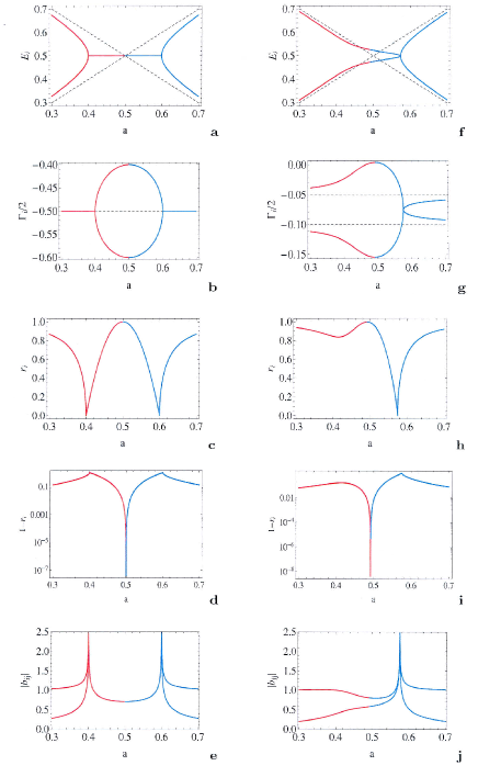
Figure 1: Energies $E_{i}$ (a,f); widths $\Gamma_{i}/2$ (b,g); phase rigidity $r_{i}$ (c,h); $1-r_{i}$ (d,i); and mixing coefficients $|b_{ij}|$ of the wavefunctions $\Phi_{i}$ and $\Phi_{j}$ of $N=2$ states coupled to a common channel as a function of $a$.
Parameters: $~{}e_{1}=1-a;~{}e_{2}=a;~{}\gamma_{1}/2=\gamma_{2}/2=-0.5;~{}\omega=0.1\,i$ (left panel) and $~{}e_{1}=1-a;~{}e_{2}=a;~{}\gamma_{1}/2=-0.05;~{}\gamma_{2}/2=-0.1;~{}\omega=0.1\,(\frac{1}{4}+\frac{3}{4}\,i)$ (right panel).
The dashed lines in (a, b, f, g) show $e_{i}(a)$ and $\gamma_{i}(a)$, respectively. The phase rigidity $r_{i}$ approaches zero at an EP, while it approaches the value one at the point of maximum width bifurcation. The eigenfunctions are mixed in both cases. When $r_{i}\to 1$, the wavefunctions are almost orthogonal. At this point, we have changed the color of the different trajectories in order to express the irreversibility of the parametric evolution up to this point (see the discussion in Sect. V).

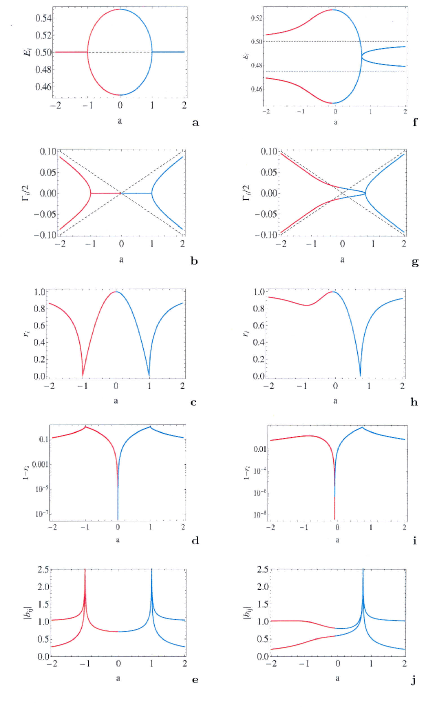
Figure 2: The same as Fig. 1 but $~{}e_{1}=e_{2}=0.5;~{}\gamma_{1}=-0.05\,a;\gamma_{2}=0.05\,a$;  $\omega=0.05$ (left panel); $~{}e_{1}=0.5;~{}e_{2}=0.475;~{}\gamma_{1}=-0.05\,a;~{}\gamma_{2}=0.05\,a$;  $\omega=0.05\,(\frac{3}{4}+\frac{1}{4}\,i)$ (right panel).
The phase rigidity $r_{i}$ approaches zero at an EP, while it approaches the value one at the point of maximum level repulsion. The results for the phase rigidity $r_{i}$ and the mixing coefficients $|b_{ij}|$ are analog to those in Fig. 1.

In order to illustrate how the states of a quantum system talk through the environment, we provide and discuss some results obtained analytically and numerically for nearby states. We start from the $2\times 2$ Hamiltonian (3) for the description of the system. First we consider a natural system with decaying states ($\gamma_{i=1,2}<0$ ;  Fig. 1) and secondly a system with loss and gain ($\gamma_{1}<0\,;~{}\gamma_{2}>0$ ;  Fig. 2). We show the real and imaginary parts ($E_{i}$ and $\Gamma_{i}$, respectively) of the eigenvalues of ${\cal H}^{(2)}$ as function of a certain parameter together with the corresponding phase rigidity $r_{i}$ of the eigenfunctions $\Phi_{i}$ and the mixing coefficients $|b_{ij}|$ of the two eigenfunctions $\Phi_{i}$ and $\Phi_{j}$ via the continuum. We choose the non-diagonal matrix elements $\omega_{12}=\omega_{21}\equiv\omega$ in (3) to be complex in Figs. 1 and 2, right panels, according to the complex coupling coefficients between system and environment in realistic systems top . For comparison with analytical results, the calculations in the left panels of Figs. 1 and 2 are performed with, respectively, imaginary and real $\omega$. In any case, the $\omega$ are fixed, i.e. they are not varied parametrically. That means, the parametrical evolution of the different values, shown in the figures, occurs without changing the coupling strength between system and environment.

Let us consider analytically the behavior that arises when the parametrical detuning of the two eigenstates of ${\cal H}^{(2)}$ is varied, bringing them towards coalescence. According to (4), the condition for coalescence reads

$$Z=\frac{1}{2}\sqrt{(e_{1}-e_{2})^{2}-\frac{1}{4}(\gamma_{1}-\gamma_{2})^{2}+i(e_{1}-e_{2})(\gamma_{1}-\gamma_{2})+4\omega^{2}}~{}=~{}0\;.$$ (16)

When $\gamma_{1}=\gamma_{2}$, and $\omega=i\,\omega_{0}$ is imaginary, it follows from (16)

$$(e_{1}-e_{2})^{2}-4\,\omega_{0}^{2} = 0~{}~{}\rightarrow~{}~{}e_{1}-e_{2}=\pm\,2\,\omega_{0}$$ (17)

such that two EPs appear. It furthermore holds

$$(e_{1}-e_{2})^{2}>4\,\omega_{0}^{2} \rightarrow ~{}Z~{}\in~{}\Re$$ (18)

$$(e_{1}-e_{2})^{2}<4\,\omega_{0}^{2} \rightarrow ~{}Z~{}\in~{}\Im$$ (19)

independent of the parameter dependence of $e_{1,2}$. According to these equations, width bifurcation of states which are nearby in energy, causes the formation of different time scales in the system. The corresponding numerical results are shown in Fig. 1 left panel. At the two EPs, $r_{i}\to 0$ and $|b_{ij}|\to\infty$. Between the two EPs, the widths bifurcate. In approaching the maximum width bifurcation (at the crossing point $e_{1}=e_{2}$), the phase rigidity of the states approaches rapidly the value $r_{i}\to 1$. That means, the wavefunctions become (almost) orthogonal at this point. This result is completely unexpected.

An analog situation occurs in the case of Fig. 2 left panel. Here, $e_{1}=e_{2}$ and $\omega$ is real. Instead of (17) to (19) we have

$$(\gamma_{1}-\gamma_{2})^{2}-16\,\omega^{2} = 0~{}~{}\rightarrow~{}~{}\gamma_{1}-\gamma_{2}=\pm\,4\,\omega$$ (20)

and

$$(\gamma_{1}-\gamma_{2})^{2}>16\,\omega^{2} \rightarrow ~{}Z~{}\in~{}\Im$$ (21)

$$(\gamma_{1}-\gamma_{2})^{2}<16\,\omega^{2} \rightarrow ~{}Z~{}\in~{}\Re\;.$$ (22)

In this case, states with comparable lifetimes repel each other in energy, see Fig. 2 left panel. Like in Fig. 1 left, $r_{i}\to 0$ and $|b_{ij}|\to\infty$ at the two EPs. Although the levels repel each other in energy between the two EPs (while their widths are equal), the phase rigidity of the states approaches rapidly the value $r_{i}\to 1$ also in this case at a critical parameter value between the two EPs. Here, level repulsion is maximum; and the wavefunctions are (almost) orthogonal. Also this result is unexpected.

The figures in the right panels of Figs. 1 and 2 show numerical results for the more realistic cases with complex coupling coefficients $\omega$. They show the same characteristic features as those in the corresponding left panels. In any case, most interesting is the parameter range between the position of an EP and that of, respectively, maximum width bifurcation and maximum level repulsion. In this parameter range, the parametrical evolution of the system is driven exclusively by the nonlinear source term of the Schrödinger equation (12) since – as mentioned above – the coupling strength $\omega$ between system and environment is fixed in the calculations. The analytical results, (17) to (22), support this statement.

In Fig. 1, we have shown the case of imaginary and almost imaginary coupling strength $\omega$ for the case of decaying states ($\gamma_{i}<0$ for $i=1,2$) and in Fig. 2 the case with real and almost real $\omega$ for the case with loss and gain ($\gamma_{1}<0,~{}\gamma_{2}>0$). The analytical and numerical results are independent of the relation between, respectively, real and imaginary $\omega$ on the one hand, and the possibility whether or not gain will take place, on the other hand.

V Discussion of the results

The results of our calculations shown in Sect. IV are performed by keeping fixed the coupling strength $\omega$ between system and environment. Width bifurcation (Fig. 1) and level repulsion (Fig. 2) can occur therefore only under the influence of the source term of the Schrödinger equation, which is nonlinear in the neighborhood of an EP, see (12). According to the results for the corresponding eigenfunctions, most interesting is the parameter range between the EP at which width bifurcation (level repulsion) starts, and that parameter value at which it becomes maximum. Here, the phase rigidity varies rapidly between its minimum and maximum values. In more detail, it vanishes at an EP according to the expectation (see section III) and increases, completely unexpected, up to its maximum value (nearly one) when width bifurcation (level repulsion) is maximum. According to the definition (15) of the phase rigidity, this means that the two eigenfunctions are (almost) orthogonal when width bifurcation (level repulsion) is maximum. Here, the eigenfunctions are mixed in the set of the original wavefunctions, what can be seen best in the results shown in the left panels of Figs. 1 and 2.

The physical meaning of this result consists in the fact that the localized part of the system gets stabilized. In the case of Fig. 1, one of the two states receives a very short lifetime due to width bifurcation, and becomes (almost) indistinguishable from the states of the environment. Although this process seems to be reversible according to the subfigures for the eigenvalues, this is in reality not the case as can be seen from the subfigures for the eigenfunctions. As mentioned above, the processes occurring in approaching $r_{k}\to 1$, take place exclusively by means of the nonlinear source term of the Schrödinger equation (12) near to an EP (since $\omega$ is fixed in the calculations). They provide states that are non-analytically connected to the original states. Due to these processes, the long-lived state has “lost” its short-lived partner with the consequence that the two original states cannot be reproduced by further variations of the parameter. The parametric evolution is irreversible. The long-lived state is more stable than the original one (according to its longer lifetime), and the system as a whole (which has lost one state) is more stable than originally. The wavefunction of this long-lived state is mixed in those of the original states.

In the case of Fig. 2, level repulsion of states with similar lifetimes causes a separation of the states in energy. Due to level repulsion, the two states separate from one another in energy, such that their interaction with one another is, eventually, of the same type as that with all the other distant states of the system. That means, each of the original states has “lost” its partner, also in this case; and the reproduction of the two originally neighbored states is prevented. As a result, the interaction of the states of the system via the environment is reduced (since all states are distant in energy). In difference to the case with width bifurcation, however, the number of states of the system as a whole remains unchanged.

According to this discussion, the results shown in Figs. 1 and 2 can be understood since the parametrical evolution of the system is irreversible (what is marked in the figures by the change of the color of all the trajectories at the final point of respective evolution). Eventually, the system as a whole is stabilized at the point of, respectively, maximum width bifurcation and maximum level repulsion; can be described quite well by a Hermitian Hamilton operator the eigenfunctions of which are orthogonal (corresponding to $r_{i}\approx 1$); and the finite lifetime of the states is hidden, to a great extent.

Thus, our results presented in Figs. 1 and 2 show the important role, which the singular EPs play in open quantum systems when the system consists of a number of neighboring, typically individual states. The parametrical evolution of a system with more than two states is studied in cluster . The irreversible processes of stabilization of the system appear also in this case. They are even stronger in the multi-level case than in the two-level case considered here. They cause, in an open quantum system, some clustering of EPs; and dynamical phase transitions occurring in a critical parameter range.

VI Relation to the phenomenon of resonance trapping

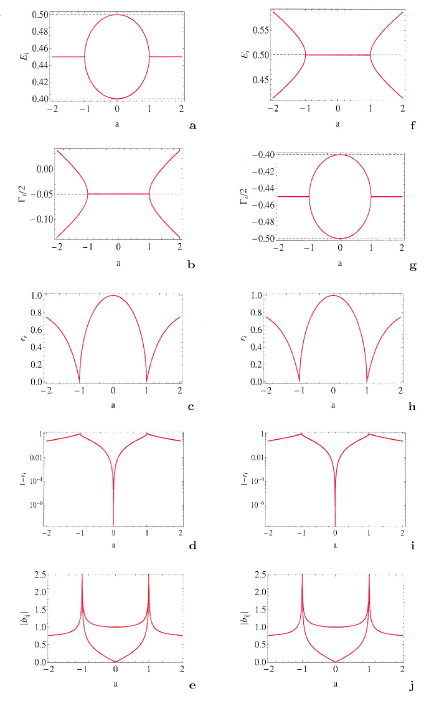
Figure 3: The same as Fig. 1 but $\omega=\omega(a)$ and fixed energies $e_{i}$ and $\gamma_{i}$.
Parameters: $e_{1}=0.5;~{}e_{2}=0.4$ and $\gamma_{1}=\gamma_{2}=-0.05$; $\omega=0.05\,a\;i$ (left); $e_{1}=e_{2}=0.5$ and $\gamma_{1}=-0.5;\gamma_{2}=-0.4$; $\omega=0.05\,a$ (right).
The dashed lines in (a, b, f, g) show $e_{i}=$ const and $\gamma_{i}=$ const, respectively. The results for the phase rigidity $r_{i}$ are analog to those in Figs. 1 and 2, while those for the mixing coefficients $|b_{ij}|$ are different. We used the same color in the whole parameter range for the different trajectories in order to express the reversible parametric evolution when $\alpha$ depends linearly on the parameter $a$ (see the discussion in the text).

The results shown in section IV and discussed in section V should not be confused with the phenomenon of resonance trapping ro91 , called also segregation of resonance widths or superradiance auerbach . This effect is known for more than 15 years and discussed controversially in literature still today. It is nothing but width bifurcation occurring in an open quantum system with many randomly distributed levels, which is described by a non-Hermitian Hamiltonian. The effect appears in a large parameter range when the coupling strength $\omega$ between system and environment is parametrically enhanced. It is difficult therefore to relate it to a phase transition. Mostly, the approximation ${\cal H}=H^{B}-i\alpha VV^{+}$ is used for the description of the system where $H^{B}$ is a Hermitian operator; $VV^{+}$ stands for the non-Hermitian perturbation; and $\alpha$ is the tuning parameter ro91 ; top ; auerbach . Eventually, long-lived trapped states are separated from the short-lived state (in the one-channel case), see e.g. harney ; jumuro . The influence of EPs is not considered in these papers since individual states are typically not looked at in these papers.

For illustration, we show in Fig. 3 numerical results for the case that $\omega$ is parametrically varied while the energies $e_{i}$ and widths $\gamma_{i}$ are fixed. The condition (16) for $Z=0$ has to be fulfilled also in this case. This causes results which are similar to those considered in detail in Eqs. (17) to (22) and in Figs. 1 and 2. Indeed, the phase rigidity approaches the value zero at an EP while it approaches the value one at the point of maximum width bifurcation and maximum level repulsion, respectively. The shape of the $r_{i}$ trajectories at the EPs is determined by the fact that the variation of $r_{i}$ occurs more slowly at one side than at the other one.

The wavefunctions of the states show, at first glance, another behavior than those in Figs. 1 and 2. The tuning parameter $\alpha$ (which characterizes the mean coupling strength of the states of the system to the environment) is assumed, usually, to be real and to increase linearly from zero up to $\infty$. At the critical value $\alpha=\alpha_{\rm cr}$, a restructuring of the system takes place jumuro ; mudiisro  : all but one state become trapped (in the one-channel case) while the width of one state increases further. Accordingly, the wavefunctions of the states are (almost) orthogonal at small $\alpha$ and become mixed beyond the restructuring (being a second-order phase transition) jumuro . This picture arises when – in addition to the eigenvalues – also the eigenfunctions are considered. It can be seen qualitatively also in Fig. 3.e : the wavefunctions are not mixed when $\alpha$ approaches zero (and the levels are distant from one another), while they become mixed when $\alpha>\alpha_{\rm cr}$ (and the widths bifurcate); see also Fig. 1 in mudiisro where the convergence of distant levels in approaching $\alpha_{\rm cr}$ is shown. In any case, the eigenfunctions are biorthogonal also for small $\alpha$ what is proven even experimentally savin .

The studies in section IV show that the nonlinear source term of the Schrödinger equation (12) strengthens and accelerates (as a function of the parameter $a$) considerably the separation of the states around an EP in energy and lifetime, respectively. The appearance of a dynamical phase transition will therefore be visible also in the representation of the results in a figure like Fig. 3 when the linear relation $\alpha\propto a$ for all $a$ (from $a=0$ to $\infty$) is replaced, at certain $a$ values, by a nonlinear one due to the nonlinear source term of the Schrödinger equation (12) near an EP. In such a case, the phase rigidity will approach quickly the value $r_{i}\approx 1$ also for large $|a|$; and $\alpha$ will not increase limitless. Correspondingly to this picture, the approximation ${\cal H}=H^{B}-i\alpha VV^{+}$ can be applied to the description of a multi-level system only near to and at the dynamical phase transition; and the states on both sides of the transition are non-analytically related to one another nearby2 .

In the paper auerbach , the wavefunctions of the states are described randomly; and the approach that $\alpha$ depends everywhere linearly on $a$, is used. The results are related to the phenomenon of superradiance; and the approach is applied to the description of different processes in physical systems, above all in nuclear physics. In celardo it is applied to the energy transport in photosynthetic light-harvesting complexes. The influence of EPs is not considered in these papers. According to our results and the discussion in Sects. IV and V, superradiance (or resonance trapping) is a clear hint to a dynamical phase transition.

VII Concluding remarks

The basic concept of our formalism is supported by many experimental results received in different physical systems, mostly in mesoscopic systems, see the review ropp . The relation between system and environment on the one hand and the measuring process on the other hand is illustrated for a mesoscopic system in Fig. 1 of ropp .

Another experimental result concerns the tunneling effect due to which, according to standard quantum mechanics, electrons can escape from atoms under the influence of strong laser fields. Recently, the tunneling delay time is measured in Helium by attosecond ionization eckle . The experimental results give a strong evidence that there is no real tunneling delay time eckle . This result is in complete agreement with (4) according to which the escape time is nothing but the imaginary part of the eigenvalue of the non-Hermitian Hamiltonian, $\Gamma_{i}\propto{\rm Im}({\cal E}_{i})$.

Whether or not the new experimental results hanson on the violation of the Bell inequality can be related to the basic assumptions of our calculations needs further investigations. See also the papers merali ; wiseman . In any case, a ’spooky action at a distance’ is possible only at and near to an EP where the interaction via the environment between two states approaches an infintely large value, as the results of our calculations show (Figs. 1 and 2).

As a conclusion we state that there are some differences between a dynamical phase transition in an open quantum system and the phenomenon of PT-symmetry breaking, in spite of many obvious similarities. The dynamical phase transition is a very general and robust phenomenon. We expect interesting results similar to those obtained for PT-symmetric systems in optics and photonics with balanced loss and gain, in the near future also in other systems.

References

- (1) C.M. Bender, Rep. Progr. Phys. 70 (2007) 947
-
(2)
A. Ruschhaupt, F. Delgado, and J. G. Muga,
J. Phys. A 38, L171 (2005);
R. El-Ganainy, K. G. Makris, D. N. Christodoulides, and Z. H. Musslimani, Optics Lett. 32, 2632 (2007);
K. G. Makris, R. El-Ganainy, D. N. Christodoulides, and Z. H. Musslimani, Phys. Rev. Lett. 100, 103904 (2008);
Z. H. Musslimani, K.G. Makris, R. El-Ganainy, and D. N. Christodoulides, Phys. Rev. Lett. 100, 030402 (2008) -
(3)
A. Guo, G.J. Salamo, D. Duchesne, R. Morandotti, M. Volatier-Ravat,
V. Aimez, G.A. Siviloglou and D.N. Christodoulides,
Phys. Rev. Lett. 103, 093902 (2009);
C.E. Rüter, K.G. Makris, R. El-Ganainy, D.N. Christodoulides, M. Segev and D. Kip, Nature Physics 6 (2010) 192;
T. Kottos, Nature Physics 6 (2010) 166 - (4) C.M. Bender, M. Gianfreda, S.K. Özdemir, B. Peng, and L. Yang, Phys. Rev. A 88, 062111 (2013)
- (5) I. Rotter, Rep. Prog. Phys. 54, 635 (1991)
- (6) N. Moiseyev, Non-Hermitian Quantum Mechanics, Cambridge University Press (2011)
- (7) N. Auerbach and V. Zelevinsky, Rep. Prog. Phys. 74, 106301 (2011)
- (8) I. Rotter, J. Phys. A 42, 153001 (2009)
-
(9)
G.A. Álvarez, E.P. Danieli, P.R. Levstein and
H.M. Pastawski, J. Chem. Phys. 124, 194507 (2006);
H.M. Pastawski, Physica B 398, 278 (2007) - (10) I. Rotter and J.P. Bird, A Review of Progress in the Physics of Open Quantum Systems: Theory and Experiment, Rep. Progr. Phys. 78 (2015) 114001
-
(11)
A. Jaouadi, M. Desouter-Lecomte, R. Lefebvre, O. Atabek,
Journ. Phys. B 46, 145402 (2013);
A. Jaouadi, M. Desouter-Lecomte, R. Lefebvre, and O. Atabek, Special Issue Quantum Physics with Non-Hermitian Operators: Theory and Experiment, Fortschr. Phys. 61, 162 (2013);
R. Lefebvre, O. Atabek, Chem. Phys. 399, 111 (2012);
O. Atabek, R. Lefebvre, M. Lepers, A. Jaouadi, O. Dulieu, V. Kokoouline, Phys. Rev. Lett. 106, 173002 (2011) -
(12)
Y. N. Joglekar, C. Thompson, D. D. Scott, and G. Vemuri,
Eur. Phys. J. Appl. Phys. 63, 30001 (2013);
A. Leclerc, G. Jolicard, and J.P. Killingbeck, J. Phys. B 46, 145503 (2013) - (13) The Nobel Prize in Physics 1963: Maria Goeppert-Mayer and J. Hans D. Jensen for their discoveries concerning nuclear structure
- (14) H. Feshbach, Ann. Phys. 5, 357 (1958); and 19, 287 (1962)
- (15) H. Eleuch and I. Rotter, Eur. Phys. J. D 69, 229 (2015)
- (16) H. Eleuch and I. Rotter, Eur. Phys. J. D 69, 230 (2015)
- (17) U. Günther, I. Rotter and B.F. Samsonov, J. Phys. A 40, 8815 (2007)
- (18) The coalescence of two eigenvalues of a non-Hermitian operator should not be confused with the degeneration of two eigenstates of a Hermitian operator. The eigenfunctions of two degenerate states are different and orthogonal while those of two coalescing states are biorthogonal and differ only by a phase, see Eqs. (5) to (14).
- (19) T. Kato, Perturbation Theory for Linear Operators, Springer, Berlin 1966
- (20) In contrast to the definition that is used in, for example, nuclear physics, we define the complex energies before and after diagonalization of by and , respectively, with and for decaying states. This definition will be useful when discussing systems with gain (positive widths) and loss (negative widths), see, e.g., top ; nearby1 .
- (21) H. Eleuch and I. Rotter, Eur. Phys. J. D 68, 74 (2014)
- (22) I. Rotter, Phys. Rev. E 64, 036213 (2001)
- (23) H. Eleuch and I. Rotter, arXiv:1506.00855v2
- (24) In studies by some other researchers, the factor in (14) does not appear. This difference is discussed in detail and compared with experimental data in the Appendix of fdp1 and in section 2.5 of top , see also Figs. 4 and 5 in berggren . Furthermore, the coalesced eigenvectors at the EP are supplemented by corresponding associated vectors defined by the Jordan chain relations, see Sect. 3 of gurosa .
- (25) I. Rotter, Special Issue Quantum Physics with Non-Hermitian Operators: Theory and Experiment, Fortschr. Phys. 61, 178 (2013)
- (26) B. Wahlstrand, I.I. Yakimenko, and K.F. Berggren, Phys. Rev. E 89, 062910 (2014)
- (27) F.M. Dittes, H.L. Harney and I. Rotter, Phys. Lett. A 153, 451 (1991)
- (28) C. Jung, M. Müller, and I. Rotter, Phys. Rev E 60, 114 (1999)
- (29) M. Müller, F.M. Dittes, W. Iskra, and I. Rotter, Phys. Rev. E 52. 5961 (1995)
- (30) J.B. Gros, U. Kuhl, O. Legrand, F. Mortessagne, E. Richalot, and D.V. Savin, Phys. Rev. Lett. 113, 224101 (2014)
-
(31)
G.L. Celardo, F. Borgonovi, M. Merkli,
V.I. Tsifrinovich, and G.P. Berman, J. Phys. Chem. C 116,
22105 (2012);
A.I. Nesterov, G.P. Berman, and A.R. Bishop, Special Issue Quantum Physics with Non-Hermitian Operators: Theory and Experiment, Fortschr. Phys. 61, 95 (2013);
D. Ferrari, G.L. Celardo, G.P. Berman, R.T. Sayre, and F. Borgonovi, J. Phys. Chem. C 118, 20 (2014) - (32) P. Eckle, A.N. Pfeiffer, C. Cirelli, A. Staudte, R. Dörner, H.G. Muller, M. Büttiker, and U. Keller, Science 322, 1525 (2008)
- (33) B. Hensen, H. Bernien, A.E. Dréau, A. Reiserer, N. Kalb, M.S. Blok, J. Ruitenberg, R.F.L. Vermeulen, R.N. Schouten, C. Abellán, W. Amaya, V. Pruneri, M.W. Mitchell, M. Markham, D.J. Twitchen, D. Elkouss, S. Wehner, T.H. Taminiau, and R. Hanson, Nature 526, 682 (2015), doi:10.1038/nature15759
- (34) Z. Merali, Nature 525, 14 (2015)
- (35) H. Wiseman, Nature 526, 649 (2015)