Multi-Target Tracking and Occlusion Handling with Learned Variational Bayesian Clusters and a Social Force Model

Abstract

This paper considers the problem of multiple human target tracking in a sequence of video data. A solution is proposed which is able to deal with the challenges of a varying number of targets, interactions and when every target gives rise to multiple measurements. The developed novel algorithm comprises variational Bayesian clustering combined with a social force model, integrated within a particle filter with an enhanced prediction step. It performs measurement-to-target association by automatically detecting the measurement relevance. The performance of the developed algorithm is evaluated over several sequences from publicly available data sets: AV16.3, CAVIAR and PETS2006, which demonstrates that the proposed algorithm successfully initializes and tracks a variable number of targets in the presence of complex occlusions. A comparison with state-of-the-art techniques due to Khan et al., Laet et al. and Czyz et al. shows improved tracking performance.

I Introduction

I-A Motivation

This paper presents a robust multiple tracking algorithm which can be used to track a variable number of people moving in a room or enclosed environment. Hence, the estimation of the unknown number of targets and their states is considered in each video frame. Multi-target tracking has many applications, such as surveillance, intelligent transportation, behavior analysis and human computer interfaces [1, 2, 3]. It is a challenging problem and a wealth of research has been undertaken to provide more efficient solutions [1, 4, 5]. Two of the major challenges associated with visual tracking of multiple targets are: 1) mitigating occlusions and 2) handling a variable number of targets. Therefore, the focus of this paper is to present a technique to robustly handle these challenges.

Overcoming occlusions is a difficult task because during an occlusion it is not possible to receive measurements originating from the occluded objects. Significant research effort has been made to address this problem, e.g. [1, 4, 6, 7].

Many 2-D tracking systems rely on appearance models of people. For instance [8] applies the kernel density approach while [9] is based on color histograms, gradients and texture models to track human objects. These techniques use template matching which is not robust to occlusions because the occluded parts of targets cannot be matched. They perform an exhaustive search for the desired target in the whole video frame which obviously requires much processing time. These techniques are also sensitive to illumination changes.

Occlusions can be handled with the help of efficient association of available data to the targets. Most of the existing multiple target tracking algorithms assume that the targets generate one measurement at a time [1, 10]. In the case of human tracking from video and many other tracking applications, targets may generate more than one measurement [4, 11]. To exploit multiple measurements, most algorithms add a preprocessing step which involves extracting features from the measurements [9]. This preprocessing step solves the problem to some extent but it results in information loss due to the dimensionality reduction and hence generally degrades the tracking results. Another problem with many of these algorithms is that they adopt the hard assignment technique [9, 12] wherein likelihood models are employed to calculate the probability of the measurements.

Recently, in [4] an approach relying on clustering and a joint probabilistic data association filter (JPDAF) was proposed to overcome occlusions. Rather than extracting features from the measurements, this approach groups the measurements into clusters and then assigns clusters to respective targets. This approach is attractive in the sense that it prevents information loss but it fails to provide a robust solution to mitigate the occlusion problem. This is because it only utilizes the location information of targets and hence the identity of individual targets is not maintained over the tracking period. As a result, the tracker may confuse two targets in close interaction, eventually causing a tracker switching problem. Other advances of such filtering approaches to multiple target tracking include multiple detection JPDAF (MD-JPDAF) [13] and interacting multiple model JPDAF (IMM-JPDAF) [14].

Interaction models have been proposed in the literature to mitigate the occlusion problem [1, 15]. The interaction model presented in [1] exploits a Markov random field approach to penalize the predicted state of particles which may cause occlusions. This approach works well for tracking multiple targets where two or more of them do not occupy the same space, but it does not address tracking failures caused by inter-target occlusions during target crossovers.

I-B Dynamic Motion Models

Dynamic models can be divided broadly into macroscopic and microscopic models [16]. Macroscopic models focus on the dynamics of a collection of targets. Microscopic models deal with the dynamics of individual targets by taking into account the behavior of every single target and how they react to the movement of other targets and static obstacles.

A representative of microscopic models is the social force model [17]. The social force model can be used to predict the motion of every individual target, i.e. the driving forces which guide the target towards a certain goal and the repulsive forces from other targets and static obstacles. A modified social force model is used in [18] and in [19] for modeling the movements of people in non-observed areas.

Many multi-target tracking algorithms in the literature only consider the case when the number of targets is known and fixed [3, 15, 12, 20]. In [1] a reversible jump Markov chain Monte Carlo (RJMCMC) sampling technique is described but in the experimental results a very strong assumption is made that the targets (ants) are restricted to enter or leave from a very small region (nest site) in a video frame. Random finite set (RFS) theory techniques have been proposed for tracking multiple targets, e.g. [21, 22], in particular the target states are considered as an RFS.

An appealing approach where the number of targets is estimated is proposed in [4] and is based on the evaluated number of clusters. Non-rigid bodies such as humans can however produce multiple clusters per target. Therefore, the number of clusters does not always remain equal to the number of targets. Hence, calculating the number of targets on the basis of the number of clusters can be inaccurate in the case of human target tracking.

I-C Main Contributions

The main contributions of this work are:

• An algorithm that provides a solution to multiple target tracking and complex inter-target interactions and occlusions. Dealing with occlusions is based on social forces between targets.

• An improved data association technique which clusters the measurements and then uses their locations and features for accurate target identification.

• A new technique based on the estimated positions of targets, size and location of the clusters, geometry of the monitored area, along with a death and birth concept to handle robustly the variable number of targets.

The framework proposed in [4] uses the JPDAF together with the variational Bayesian clustering technique for data association and a simple dynamic model for state transition. Our proposed technique differs from that of [4] in three main aspects: 1) in the dynamic model which is based on social forces between targets, 2) a new features based data association technique, and 3) a new technique for estimation of number of targets which is based on the information from clusters, position of existing targets and geometry of monitored area location.

The remainder of the paper is organized as follows: Section II describes the proposed algorithm, Section III presents the proposed data association algorithm, Section IV explains the clustering process and Section V describes the proposed technique for estimating the number of targets. Extensive experimental validation is given in Section VI. Section VII contains discussion and finally, conclusions are presented in Section VIII.

II The Proposed Algorithm

II-A Bayesian estimation

The goal of the multi-target tracking process is to track the state of $N$ unknown targets. The state of each target is represented as ${\bf x}^{i}_{k},\,(i=1,\ldots,N)$, which is a column vector containing the position and velocity information of the $i^{th}$ target at time $k$. The joint state of all the targets is constructed as the concatenation of the individual target states $\mathbf{x}_{k}=[({\bf x}^{1}_{k})^{T},\ldots,({\bf x}^{i}_{k})^{T},\ldots,({\bf x}^{N}_{k})^{T}]^{T}$, where $(\cdot)^{T}$ denotes the transpose operator. Measurements at time $k$ are represented as $\mathbf{{y}}_{k}=[({\bf{y}}^{1}_{k})^{T},\ldots,({\bf{y}}^{j}_{k})^{T},\ldots,({\bf{y}}^{L}_{k})^{T}]^{T}$, where ${\bf{y}}^{j}_{k}$ is described in Section II-B.

Within the Bayesian framework, the tracking problem consists of estimating the belief of the state vector $\mathbf{x}_{k}$ given the measurement vector $\mathbf{{y}}_{1:k}$. The objective is to sequentially estimate the posterior probability distribution $p(\mathbf{x}_{k}|\mathbf{y}_{1:k})$ at every time step $k$. The posterior state distribution $p(\mathbf{x}_{k}|\mathbf{y}_{1:k})$ can be estimated in two steps. First, the prediction step [23] is

$$p({\bf x}_{k}|{\bf{y}}_{1:k-1})=\int p({\bf x}_{k}|{\bf x}_{k-1})p({\bf x}_{k-1}|{\bf{y}}_{1:k-1})d{\bf x}_{k-1},$$ (1)

where $p({\bf x}_{k}|{\bf x}_{k-1})$ is the state transition probability. After the arrival of the latest measurements, the update step becomes

$$p({\bf x}_{k}|{\bf{y}}_{1:k})=\frac{p({\bf{y}}_{k}|{\bf x}_{k})p({\bf x}_{k}|{\bf{y}}_{1:k-1})}{p({\bf{y}}_{k}|{\bf{y}}_{1:k-1})},$$ (2)

where $p({\bf{y}}_{k}|{\bf x}_{k})$ is the measurement likelihood function.

The two step tracking process yields a closed form expression only for linear and Gaussian dynamic models [10]. Particle filtering [23] is a popular solution for suboptimal estimation of the posterior distribution $p(\mathbf{x}_{k}|\mathbf{{y}}_{1:k})$, especially in the nonlinear and non-Gaussian case. The posterior state distribution is estimated by a set of random samples ${\bf x}_{k}^{s}$, $s=1,\ldots,N_{s}$ and their associated weights ${w}^{s}_{k}$ at time $k$

$$p({\bf x}_{k}|{\bf{y}}_{1:k})\approx\sum_{s=1}^{N_{s}}{w}^{s}_{k}\delta({\bf x}_{k}-{\bf x}_{k}^{s}),$$ (3)

where $N_{s}$ is the total number of particles and $\delta(\cdot)$ denotes a multivariate Dirac delta function.

We apply particle filtering within the JPDAF framework to estimate the states of targets. The JPDAF recursively updates the marginal posterior distribution $p({\bf x}_{k}^{i}|{\bf{y}}_{1:k})$ for each target. In our work, given the state vector ${\bf x}^{i}_{k-1}$ of target $i$, the next set of particles at time step $k$ is predicted by the social force dynamic model (equations (6)-(9)) which is described later in Section II-C. The state transition model is represented by equation (9). The $N_{s}$ particles and their corresponding weights can approximate the marginal posterior at time step $k$.

To assign weights to each sample we follow the likelihood model along with the data association framework which is explained in Section III.

II-B Measurement Model

The algorithm considers $L$ number of pixels in a single video frame captured by one camera as input measurements. From the sequentially arriving video frames, the silhouette of the moving targets (foreground) is obtained by background subtraction [24]. At time $k$, the measurement vector is: $\mathbf{y}_{k}=[({\bf y}^{1}_{k})^{T},\ldots,({\bf y}^{j}_{k})^{T},\ldots,({\bf y}^{L}_{k})^{T}]^{T}$. The state $\mathbf{x}_{k}$ at time $k$ is estimated by using the measurement vector

$${\bf{y}}_{k}=h_{k}(\mathbf{x}_{k},{\bf e}_{m,k}),$$ (4)

where ${\bf e}_{m,k}$ is the measurement noise vector. After the background subtraction [24], the measurements at time $k$ are: $\tilde{\mathbf{y}}_{k}=[(\tilde{{\bf y}}^{1}_{k})^{T},\ldots,(\tilde{{\bf y}}^{j}_{k})^{T},\ldots,(\tilde{{\bf y}}^{M}_{k})^{T}]^{T}$, which are assumed to correspond to the moving targets (please see Section VI for details). The measurement function $h_{k}(\cdot)$ is represented by some features of the video frames, e.g. the color histogram. The measurement vector $\tilde{\mathbf{y}}_{k}$ contains only a set of foreground pixels. After background subtraction the number of pixels with non-zero intensity values is reduced to $M$, where $M<<L$. The number of foreground pixels $M$ is variable over time.

The background subtracted silhouette regions are clustered with the variational Bayesian algorithm described in Section IV. During the clustering process each data point (pixel) ${\tilde{\bf{y}}}^{j}_{k}$ contains only the coordinates of the pixel. During the data association stage we use the red, green, blue (RGB) color information contained in each pixel to extract color features of a cluster.

II-C The Social Force Model

The system dynamics model is defined by the following equation

$$\mathbf{x}_{k}=f_{k}(\mathbf{x}_{k-1},{\boldsymbol{\xi}}_{k-1}),$$ (5)

where ${\boldsymbol{\xi}}_{k-1}$ is the system noise vector. Under the Markovian assumption our state transition model for the $i^{th}$ target is represented as $p({\bf x}^{i}_{k}|{\bf x}^{i}_{k-1},\mathcal{F}_{i})$, where $\mathcal{F}_{i}$ is the social force being applied on target $i$.

The motion of every target can be influenced by a number of factors, e.g. by the presence of other targets and static obstacles. The interactions between them are modeled here by means of a social force model [17], the key idea of which is to calculate attraction and repulsion forces which represent the social behavior of humans. The so-called “social forces” depend on the distances between the targets.

Following Newtonian dynamics, a change of states stems from the existence of exterior forces. Given a target $i$, the total number of targets that influence target $i$ at time $k$, is $N_{i}$. The overall force ${\bf\mathcal{F}}_{i}$ applied on target $i$ is the sum of the forces exerted by all the neighboring targets, ${\bf\mathcal{F}}_{i}=\sum_{j\in N_{i}}{\bf\mathcal{F}}_{j}$. Most of the existing force based models [17] consider only repulsive forces between targets to avoid collisions. However, in reality there can be many other types of social forces between targets due to different social behavior of targets, for instance attraction, spreading and following [25].

Suppose a target $i$ at time step $k$ has $N_{i}$ neighbors, therefore, it would have $N_{i}$ links with other targets $l=1\ldots N_{i}$. Only those targets are considered as neighbors of target $i$ which are within a threshold distance $\hat{d}$ from $i$. We consider that a social behavior over link $l$ is given by $\varphi_{l}\in\{1\ldots\Gamma\}$ where $\Gamma$ is the total number of social behaviors. An interaction mode vector $\boldsymbol{\varphi}_{i}~{}=~{}[\varphi_{1},\varphi_{2},\ldots,\varphi_{N_{i}}]$ for target $i$ is a vector comprising the different social behaviors over all the links. The total number of interaction modes is $S=\Gamma^{N_{i}}$.

A force due to one interaction mode is calculated as a sum of forces over all the social links

$$\mathcal{F}(\boldsymbol{\varphi}_{i})=\sum_{l=1}^{N_{i}}\phi^{l},$$ (6)

where $\mathcal{F}(\boldsymbol{\varphi}_{i})$ is the force due to social mode $\boldsymbol{\varphi}_{i}$ and $\phi^{l}$ is the force over the link $l$. In our work we consider three social forces: repulsion, attraction and non-interaction. These broadly encompass all possible human motions.

People naturally tend to avoid collisions between each other. This is reflected by repulsion forces. Attraction accounts for the behaviors when people approach each other for the intention of meeting, this behavior is usually ignored in the existing force based models. The non-interactions mode represents the behavior of independent motion of every person.

The repulsive force applied by target $j$ on target $i$ over the link $l$ is calculated as [25]

$$\phi_{-}^{l}=f_{r}\exp\biggr{(}\frac{r^{l}_{ij}-d^{l}_{ij}}{b}\biggr{)}{\bf u}_{ji},$$ (7)

when $d^{l}_{ij}$ is less than an empirically found threshold $\hat{d}$, defined as $3m$ in Table I in Section VI-E; where $b$ which is set equal to $\hat{d}$ is the boundary in which a target $j$ has its influence of force on target $i$. The Euclidean distance between targets $i$ and $j$ over link $l$ is defined as $d^{l}_{ij}$, $r^{l}_{ij}=r^{l}_{i}+r^{l}_{j}$ is the sum of radii of influence of targets $i$ and $j$ over link $l$ and $f_{r}$ is the magnitude of the repulsive force. The unit vector from target $j$ to target $i$ is represented as ${\bf u}_{ji}$.

When targets approach each other, repulsive forces act, to avoid collisions. The repulsive force therefore increases as described by equation (7). Similarly, when targets move apart the repulsion decreases because it is less likely for a collision to occur, and therefore they tend to come closer to each other. Attraction is a phenomenon opposite to repulsion. When targets move apart, they tend to attract each other for the intension of meeting and when they move closer, the repulsion increases which means they are less attracted. This attraction phenomenon is described by equation (8). However, if targets are at a distance more than a threshold, it can be assumed they do not influence each other.

An attractive force applied by target $j$ on target $i$ over the link $l$ is calculated as [25]

$$\phi_{+}^{l}=f_{a}exp\biggr{(}-\frac{(r_{ij}^{l}-d_{ij}^{l})}{b}\biggr{)}{\bf u}_{ij},$$ (8)

when $d_{ij}^{l}$ is less than an empirically found threshold $\hat{d}$, defined as $3m$ in Table I in Section VI-E, where $f_{a}$ is the magnitude of the attractive force and force due to non-interactions is considered to be zero.

To represent the state ${\bf x}_{k}$ of targets at every time step $k$, a pixel coordinate system is used. Since, our state transition equation (9) below is based on the social force model, to predict the new particles ${\bf x}_{k}^{s}$, position and velocity values contained within the state vector ${\bf x}_{k-1}$ and the particles at time step $k-1$ are converted to the image ground coordinate system (a process known as homography [26]). After predicting the new set of $N_{s}$ particles for state ${\bf x}_{k}$ these particles are converted back to pixel coordinates. For conversion between the two coordinate systems the four point homography technique is implemented, as used in [27]. The position and velocity at time step $k$ in pixel coordinates are represented as ${\bf p}_{k}$ and ${\bf v}_{k}$, respectively, whereas, the position and velocity in ground coordinates systems are represented as $\tilde{\bf p}_{k}$ and $\tilde{\bf v}_{k}$ respectively. At every time step a new state is predicted with respect to interaction mode $\boldsymbol{\varphi}_{i}$ according to the following model [25]

$$\biggr{[}\begin{matrix}\tilde{\bf p}_{k}(\boldsymbol{\varphi}_{i})\\ \tilde{\bf v}_{k}(\boldsymbol{\varphi}_{i})\end{matrix}\biggr{]}=\biggr{[}\begin{matrix}\tilde{\bf p}_{k-1}(\boldsymbol{\varphi}_{i})+\tilde{\bf v}_{k-1}\Delta t+\frac{1}{2}\frac{{\bf\mathcal{F}}(\boldsymbol{\varphi}_{i})}{m}\Delta t^{2}\\ \tilde{\bf v}_{k-1}(\boldsymbol{\varphi}_{i})+\frac{\mathcal{F}(\boldsymbol{\varphi}_{i})}{m}\Delta t\end{matrix}\biggr{]}+{\boldsymbol{\xi}}_{k},$$ (9)

where $\Delta t$ is the time interval between two frames, $m$ represents mass of the target and ${\boldsymbol{\xi}}_{k}$ is the system noise vector.

The social force model gives more accurate predictions than the commonly used constant velocity model [28] and helps tracking objects in the presence of close interaction. This cannot be done with a simple constant velocity motion model.

The implementation of the force model is further explained in Algorithm 1 at the end of the next section.

III Data Association and Likelihood

To deal with the data association problem we represent a measurement to target $(M\rightarrow T)$ association hypothesis by the parameter $\boldsymbol{\psi}_{k}$, whereas $\boldsymbol{\Psi}_{k}$ represents the set of all hypotheses. At this stage we assume that one target can generate one measurement. However, later in this section we relax this assumption and develop a data association technique for associating multiple measurements (clusters of measurements) to one target. If we assume that measurements are independent of each other then the likelihood model conditioned on the state ${\bf x}_{k}$ of targets and measurement to target association hypothesis $\boldsymbol{\psi}_{k}$ can be represented as in [10] (equation (11))

$$p({\bf{y}}_{k}|{\bf x}_{k},\boldsymbol{\psi}_{k})=\prod_{{j^{\prime}}\in\mathcal{\boldsymbol{J}}_{o}}p_{c}({\bf{y}}_{k}^{j^{\prime}})\prod_{j\in\mathcal{\boldsymbol{J}}}p_{t}({\bf{y}}_{k}^{j}|{\bf x}_{k}^{i,j}),$$ (10)

where $\mathcal{\boldsymbol{J}}_{o}$ and $\mathcal{\boldsymbol{J}}$ are, respectively, measurement indices sets, corresponding to the clutter measurements and measurements from the targets to be tracked, for convenance of notation the time dependence is not shown on these quantities. The terms $p_{c}(\cdot)$ and $p_{t}(\cdot)$ are characterizing, respectively, the clutter likelihood and the measurement likelihood association to each target $i$ whose state is represented as ${\bf x}_{k}^{i,j}$. If we assume that the clutter likelihood $p_{c}(\cdot)$ is uniform over the volume $\gamma$ of the measurement space and ${f_{k}}$ represents the total number of clutter measurements, then the probability $p({\bf{y}}_{k}|{\bf x}_{k},\boldsymbol{\psi}_{k})$ can be represented as

$$p({\bf{y}}_{k}|{\bf x}_{k},\boldsymbol{\psi}_{k})=\gamma^{f_{k}}\prod_{j\in\mathcal{\boldsymbol{J}}}p_{t}({\bf{y}}_{k}^{j}|{\bf x}_{k}^{i,j}).$$ (11)

The form of $p_{t}({\bf{y}}_{k}^{j}|{\bf x}_{k}^{i,j})$ is given in Section III-C.

III-A The JPDAF Framework

The standard JPDAF algorithm estimates the marginal distribution of each target by following the prediction and update process described in equations (1) and (2). In the development below, we exploit the framework from [10]. The prediction step for each target independently becomes

$$p({\bf x}^{i}_{k}|{\bf{y}}_{1:k-1})=\int p({\bf x}^{i}_{k}|{\bf x}^{i}_{k-1})p({\bf x}^{i}_{k-1}|{\bf{y}}_{1:k-1})d{\bf x}^{i}_{k-1},$$ (12)

where we assume that the prediction at time step $k$ is based on the measurements only at $k-1$. The JPDAF defines the likelihood of measurements with respect to target $i$ as in [10] (equation (25))

$$p({\bf y}_{k}|{\bf x}_{k}^{i})={\mathcal{A}}_{k}^{i,o}+\sum_{j=1}^{L}{\mathcal{A}}_{k}^{i,j}p({\bf y}^{j}_{k}|{\bf x}_{k}^{i}),$$ (13)

where ${\mathcal{A}}_{k}^{i,j}$ is the association probability that the $i^{th}$ target is associated with the $j^{th}$ measurement and ${\mathcal{A}}_{k}^{i,o}$ is the association probability that the target $i$ remains undetected; for notational convenience, in equation (13) and the remainder of the paper we drop the subscript $t$ on the target likelihood.With prediction and likelihood functions defined by equations (12) and (13), respectively, the JPDAF estimates the posterior probability of the state of target $i$

$$p({\bf x}^{i}_{k}|{\bf{y}}_{1:k})\propto p({\bf{y}}_{k}|{\bf x}^{i}_{k})p({\bf x}^{i}_{k}|{\bf{y}}_{1:k-1}).$$ (14)

The association probability ${\mathcal{A}}_{k}^{i,j}$ can be defined as in [10] (equation (27))

$${\mathcal{A}}_{k}^{i,j}=\sum_{\boldsymbol{\psi}_{k}\in\boldsymbol{\Psi}_{k}^{i,j}}p(\boldsymbol{\psi}_{k}|{\bf{y}}_{1:k}),$$ (15)

where $\boldsymbol{\Psi}_{k}^{i,j}$ represents the set of all those hypotheses which associate the $j^{th}$ measurement to the $i^{th}$ target. The probability $p(\boldsymbol{\psi}_{k}|{\bf{y}}_{1:k})$ can be represented as equation (28) in [10]

$$p(\boldsymbol{\psi}_{k}|{\bf{y}}_{1:k})\propto p(\boldsymbol{\psi}_{k}|{\bf x}_{k})\gamma^{f_{k}}\prod_{j\in\mathcal{\boldsymbol{J}}}p({\bf{y}}^{j}_{k}|{\bf{y}}_{1:k-1}),$$ (16)

where $p(\boldsymbol{\psi}_{k}|{\bf x}_{k})$ is the probability of assignment $\boldsymbol{\psi}_{k}$ given the current state of the objects. We assume that all assignments have equal prior probability and hence $p(\boldsymbol{\psi}_{k}|{\bf x}_{k})$ can be approximated by a constant. If we define a normalizing constant $\pi$ ensuring that $p(\boldsymbol{\psi}_{k}|{\bf{y}}_{1:k})$ integrates to one and define the predictive likelihood $p({\bf{y}}^{j}_{k}|{\bf{y}}_{1:k-1})$ as

$$\begin{split}p({\bf{y}}^{j}_{k}|{\bf{y}}_{1:k-1})=\int p({\bf{y}}_{k}^{j}|{\bf x}_{k}^{i})p({\bf x}_{k}^{i}|{\bf{y}}_{1:k-1})d{\bf x}_{k}^{i},\end{split}$$ (17)

then equation (16) becomes

$$p(\boldsymbol{\psi}_{k}|{\bf{y}}_{1:k})\!=\!\pi\gamma^{f_{k}}\!\!\!\prod_{(j,i)\in\boldsymbol{\psi}_{k}}\!\int\!\!p({\bf{y}}_{k}^{j}|{\bf x}_{k}^{i})p({\bf x}_{k}^{i}|{\bf{y}}_{1:k-1})d{\bf x}_{k}^{i}.$$ (18)

III-B Particle Filtering Based Approach

The standard JPDAF assumes a Gaussian marginal filtering distribution of the individual targets [28, 10]. In this paper we adopt a particle filtering based approach which represents the state of every target with the help of samples. Therefore, we modify equation (18) as

$$p(\boldsymbol{\psi}_{k}|{\bf{y}}_{1:k})=\pi\gamma^{f_{k}}\prod_{(j,i)\in\boldsymbol{\psi}_{k}}\sum_{s=1}^{N_{s}}\hat{w}^{i,s}_{k}p({\bf{y}}_{k}^{j}|{\bf x}_{k}^{i,s}),$$ (19)

where $N_{s}$ is the total number of particles which are required to estimate the filtering distribution over every individual target and $\hat{w}^{i,s}_{k}$ represents the associated predictive weights as described in [10]. We can modify equation (19) as

$$p(\boldsymbol{\psi}_{k}|{\bf{y}}_{1:k})=\pi\gamma^{f_{k}}\prod_{(j,i)\in\boldsymbol{\psi}_{k}}\frac{1}{N_{s}}\sum_{s=1}^{N_{s}}p({\bf{y}}_{k}^{j}|{\bf x}_{k}^{i,s}).$$ (20)

Once the probability $p(\boldsymbol{\psi}_{k}|{\bf{y}}_{1:k})$ is calculated according to (20), we can substitute it in equation (15) to calculate the association probability. We can further use this association probability to calculate the measurement likelihood from equation (13).

After drawing particles from a suitably constructed proposal distribution [23], the weights associated with particles are calculated, $\hat{w}^{i,s}_{k}=p({\bf y}_{k}|{\bf x}_{k}^{i})$. The particles and their weights can then be used to approximate the posterior distribution

$$p({\bf x}^{i}_{k}|{\bf{y}}_{1:k})\approx\sum_{s=1}^{N_{s}}{w}^{i,s}_{k}\delta({\bf x}^{i}_{k}-{\bf x}_{k}^{i,s}),$$ (21)

for individual targets where ${\bf x}_{k}^{i,s}$ is the $s^{th}$ particle for target $i$ and ${w}^{i,s}_{k}$ is the associated weight. For estimation of a state we predict $N_{\varphi}$ particles with respect to every interaction mode. There are $S$ interaction modes, therefore, $N_{s}=S\times N_{\varphi}$ represents the total number of samples.

III-C Algorithm to Associate Multiple Measurements to a Target

In the case of tracking people in video, every person generates multiple measurements. To avoid any information loss we relax the assumption that every person can generate a single measurement. Here we present a data association technique for associating multiple measurements to every target. To achieve this, the algorithm groups the foreground pixels into clusters with the help of a variational Bayesian clustering technique, and then instead of associating one measurement to one target we associate clusters to every target. The clustering process returns $\kappa$ clusters, where the number of clusters is not predefined or fixed. Clusters at discrete time $k$ are regions represented as ${\bf Z}^{1}_{k},{\bf Z}^{q}_{k},\ldots,{\bf Z}^{\kappa}_{k}$, where ${\bf Z}^{q}_{k}$ is the $q^{th}$ cluster which contains certain measurements, i.e. a number of vectors ${\tilde{\bf y}}_{k}^{j}$ of foreground pixels. The complete clustering process is described in Section IV. The clustering process aims to assign measurements to the respective clusters and gives as output a correspondence matrix ${\bf B}_{k}=[({\bf b}_{k}^{1})^{T},\ldots,({\bf b}_{k}^{j})^{T},\ldots,({\bf b}_{k}^{M})^{T}]^{T}$, where ${\bf b}_{k}^{j}=[b_{k}^{j,1},b_{k}^{j,2},\ldots,b_{k}^{j,q},\ldots,b_{k}^{j,\kappa}]$ indicates, at discrete time $k$, to which cluster, the measurement vector ${\tilde{\bf y}}_{k}^{j}$ corresponds. All but one of the elements of ${\bf b}_{k}^{j}$ is zero, if e.g. ${\tilde{\bf y}}_{k}^{j}$ belongs to the $q^{th}$ cluster then the correspondence vector will be, ${\bf b}_{k}^{j}=[0,\ldots,0,1,0,\ldots,0]$, which shows only the $q^{th}$ element of ${\bf b}_{k}^{j}$ is nonzero. Please note that from this section onwards all equations are written with respect to the measurement vector $\tilde{\bf y}_{k}$ that contains foreground pixels.

We modify the measurement to target $(M\rightarrow T)$ association probability ${\mathcal{A}}_{k}^{i,j}$ to calculate the cluster to target $(Z\rightarrow T)$ association probability ${\mathcal{A}}_{k}^{i,q}$, where $q$ represents the cluster index

$${\mathcal{A}}_{k}^{i,q}=\sum_{\boldsymbol{\psi}_{k}\in\boldsymbol{\Psi}_{k}^{i,q}}p(\boldsymbol{\psi}_{k}|\tilde{\bf{y}}_{1:k}),$$ (22)

where $\boldsymbol{\Psi}_{k}^{i,q}$ represents the set of all those hypotheses which associate the $q^{th}$ cluster to the $i^{th}$ target. We modify equation (20) to define the probability $p(\boldsymbol{\psi}_{k}|\tilde{\bf{y}}_{1:k})$ as

$$p(\boldsymbol{\psi}_{k}|\tilde{\bf{y}}_{1:k})=\pi\gamma^{f_{k}}\!\!\prod_{(q,i)\in\boldsymbol{\psi}_{k}}\,\,\prod_{{\tilde{\bf y}}_{k}^{j}:b_{k}^{j,q}=1}\!\!\frac{1}{N_{s}}\!\!\sum_{s=1}^{N_{s}}p(\tilde{\bf{y}}_{k}^{j}|{\bf x}_{k}^{i,s}),$$ (23)

where ${\tilde{\bf y}}_{k}^{j}:b_{k}^{j,q}=1$ represents only those measurements which are associated with cluster $q$. The measurement likelihood defined in equation (13) is modified as follows

$$\begin{split}p(\tilde{\bf y}_{k}|{\bf x}_{k}^{i,s})={\mathcal{A}}_{k}^{i,o}+\sum_{j=1}^{M}{\mathcal{A}}_{k}^{i,(q:b_{k}^{j,q}=1)}p(\tilde{\bf y}^{j}_{k}|{\bf x}_{k}^{i,s}),\end{split}$$ (24)

where $q:b_{k}^{j,q}=1$ represents that the $j^{th}$ measurement is associated with the $q^{th}$ cluster and ${\mathcal{A}}_{k}^{i,o}$ represents the probability that the cluster is not associated to the $i^{th}$ target and ${\mathcal{A}}_{k}^{i,(q:b_{k}^{j,q}=1)}$ is the probability that the cluster is associated to the $i^{th}$ target. To limit the number of hypotheses when the number of targets increases, we have adopted Murty’s algorithm [29]. This algorithm returns the $k$-best hypotheses. The elements of the cost matrix for Murty’s algorithm are calculated with the particles ${\bf x}_{k}^{i,s}$

$$cost_{q}^{i}=\prod_{{\tilde{\bf y}}_{k}^{j}:b_{k}^{j,q}=1}\frac{1}{N_{s}}\sum_{s=1}^{N_{s}}p(\tilde{\bf{y}}_{k}^{j}|{\bf x}_{k}^{i,s}),$$ (25)

where $cost_{q}^{i}$ represents the cost of assigning the $q^{th}$ cluster to the $i^{th}$ target.

The JPDAF [30] data association technique proposed in [4] performs well when two targets do not undergo a full occlusion. However, this data association technique sometimes fails to associate measurements correctly, especially when two or more targets partially occlude each other or when targets come out of full occlusion. This is due to the fact that this data association is performed on the basis of location information without any information about the features of targets. This can result in missed detections and wrong identifications.

In order to cope with these challenges under occlusions, a data association technique is proposed which assigns clusters to targets by exploiting both location and features of clusters. First, we define the term $\prod_{{\tilde{\bf y}}_{k}^{j}:b_{k}^{j,q}=1}\frac{1}{N_{s}}\sum_{s=1}^{N_{s}}p(\tilde{\bf{y}}_{k}^{j}|{\bf x}_{k}^{i,s})$ in equation (23) as follows

$$\begin{split}\!\!\!\prod_{{\tilde{\bf y}}_{k}^{j}:b_{k}^{j,q}=1}\!\!\!\frac{1}{N_{s}}\!\!\sum_{s=1}^{N_{s}}\!p(\tilde{\bf{y}}_{k}^{j}|{\bf x}_{k}^{i,s})\!=\!\!{p({\bf Z}_{k}^{q}|{\bf x}_{k}^{i,s})}\!\!\!\!\!\!\!\prod_{{\tilde{\bf y}}_{k}^{j}:b_{k}^{j,q}=1}\!\!\!\!\frac{1}{N_{s}}\sum_{s=1}^{N_{s}}\!\!\mathcal{N}(\tilde{\bf{y}}_{k}^{j}|\boldsymbol{\mu}_{s},{\bf\!\Sigma}_{s}\!),\end{split}$$ (26)

where $\boldsymbol{\mu}_{s}={\bf x}_{k}^{i,s}$ is the mean vector and ${\bf\Sigma}_{s}$ is the fixed and known diagonal covariance matrix. The association probability ${p({\bf Z}_{k}^{q}|{\bf x}_{k}^{i,s})}$ in equation (26) is calculated by extracting features from the clusters at time step $k$ and comparing them with a reference feature (template) of target $i$. The reference feature for target $i$ is extracted when it first appears in the monitored area. To improve the computational efficiency, the probability $p({\bf Z}_{k}^{q}|{\bf x}_{k}^{i,s})$ is calculated only when targets approach each other. This association probability is defined as

$$p({\bf Z}_{k}^{q}|{\bf x}_{k}^{i,s})\!=\!\!\left\{\begin{array}[]{ll}\!\!\!\!\exp\biggr{(}\!\!-\frac{d^{i}(H^{i}_{ref},H^{q}_{k})}{2{\bf\sigma}^{2}}\biggr{)}&\!\!\!\textrm{if}~{}P_{occlusion}^{i}\!>\!\vartheta\\ \!\!\!\!1&\!\!\!\!\textrm{otherwise}\end{array}\right.$$ (27)

where ${\bf\sigma}^{2}$ is the measurement noise variance, $H^{i}_{ref}$ and $H^{q}_{k}$ are histograms of features of the $i^{th}$ target and $q^{th}$ cluster, respectively and $d^{i}(H^{i}_{ref},H^{q}_{k})$ is the distance between them. One possible option is to use the Bhattacharyya distance [31]. The parameter $\vartheta$ is a predefined threshold, and the probability of occlusion is defined as

$$P_{occlusion}^{i}=\exp\biggr{(}-\frac{d^{i}_{min}}{\Delta_{c}}\biggr{)},$$ (28)

where $d^{i}_{min}$ is the minimum Euclidean distance among a set of distances which is calculated for target $i$ from all other targets at time $k$,

$$d^{i}_{min}=\min\limits_{i\neq n}{\{d_{i,n}\}},$$ (29)

and $\Delta_{c}$ is the distance constant which limits the influence of target $n$ on target $i$. A higher value of minimum distance $d^{i}_{min}$ results in a smaller value of probability of occlusions and when this probability drops below threshold $\vartheta$ the probability $p({\bf Z}_{k}^{q}|{\bf x}_{k}^{i,s})$ becomes unity.

Algorithm 1 The social force model

Input: $N_{s}$ particles and the state of targets at time step $k-1$
Output: $N_{s}$ particles for time step $k$

1:  Convert the state at $k-1$ from pixel coordinates system to real world ground coordinates.

2:  Use ground coordinates to calculate distances between targets.

3:  Based on distances create links between targets.

4:  for $i=1,...,N$(where $N$ is the number of targets) do

5:     Create $S=\Gamma^{N_{i}}$ social modes

6:     Calculate forces due to every social mode by using equations (6), (7) and (8).

7:     for $s=1:\Gamma^{N_{i}}:N_{s}$(where $N_{s}$ is the number of particles) do

8:        Convert the particle ${\bf x}_{k-1}^{i,s}$ to the ground plane.

9:        Add random noise to get ${\bf x}_{k-1}^{i,s}+{\boldsymbol{\xi}}_{k-1}$ .

10:        for $s_{\boldsymbol{\varphi}_{i}}=1,...,\Gamma^{N_{i}}$ do

11:           Predict particle ${\bf x}_{k-1}^{i,s+s_{\boldsymbol{\varphi}_{i}}-1}$ by using particle ${\bf x}_{k-1}^{i,s}+{\boldsymbol{\xi}}_{k-1}$ w.r.t. the social mode $\boldsymbol{\varphi}_{i}$ in equation (9).

12:           Convert the particle ${\bf x}_{k-1}^{i,s+s_{\boldsymbol{\varphi}_{i}}-1}$ to the pixel coordinates.

13:        end for

14:     end for

15:  end for

IV Variational Bayesian Clustering - from Measurements to Clusters

The clustering process aims to subdivide the foreground image into regions corresponding to the different targets. A variational Bayesian clustering technique is developed to group the $M$ foreground pixels into $\kappa$ clusters. Each cluster at time index $k$ is represented by its center ${\bf{\boldsymbol{\mu}}}_{k}^{q}$, where $q=1,\ldots,\kappa$. A binary indicator variable $b_{k}^{j,q}\in\{0,1\}$ represents to which of the $q^{th}$ clusters data point $\tilde{\bf{y}}_{k}^{j}$ is assigned; for example, when the data point $\tilde{\bf{y}}_{k}^{j}$ is assigned to the $q^{th}$ cluster then $b_{k}^{j,q}=1$, and $b_{k}^{j,l}=0$ for $l\neq q$.

We assume that the foreground pixel locations are modeled by a mixture of Gaussian distributions. The clustering task can be viewed as fitting mixtures of Gaussian distributions [32] to the foreground measurements. Every cluster ${\bf Z}_{k}^{q}$ of foreground pixel locations is assumed to be modeled by a Gaussian distribution, $\mathcal{N}(\tilde{\bf{y}}_{k}^{j}|{\boldsymbol{\mu}}_{k}^{q},{\bf\Sigma}_{k}^{q})$ which is one component of the mixture of Gaussian distributions. Each cluster has a mean vector ${\boldsymbol{\mu}}_{k}^{q}$ and a covariance matrix ${\boldsymbol{\Sigma}}_{k}^{q}$. Hence, the probability of a data point $\tilde{\bf{y}}^{j}_{k}$ can be represented as

$$p(\tilde{\bf{y}}_{k}^{j}|{\bf C}_{k},{\boldsymbol{\mu}}_{k},{\bf\Sigma}_{k})=\sum_{q=1}^{\kappa}C_{k}^{q}\mathcal{N}(\tilde{\bf{y}}_{k}^{j}|{\boldsymbol{\mu}}_{k}^{q},{\bf\Sigma}_{k}^{q}),$$ (30)

where $\boldsymbol{\mu}_{k}=\{\boldsymbol{\mu}_{k}^{q}\}_{q=1}^{\kappa}$ and $\boldsymbol{\Sigma}_{k}=\{\boldsymbol{\Sigma}_{k}^{q}\}_{q=1}^{\kappa}$. The mixing coefficient vector is defined as ${\bf C}_{k}=[C_{k}^{1},\ldots,C_{k}^{q},\ldots,C_{k}^{\kappa}]^{T}$, where $C_{k}^{q}$ represents the probability of selecting the $q^{th}$ component of the mixture which is the probability of assigning the $j^{th}$ measurement to the $q^{th}$ cluster. If we assume that all the measurements are independent, then the log likelihood function becomes [32]

$$\ln p(\tilde{\bf{y}}_{k}|{\bf C}_{k},{\boldsymbol{\mu}}_{k},{\bf\Sigma}_{k})\!\!=\!\!\sum_{j=1}^{M}\!\ln\biggr{\{}\!\!\sum_{q=1}^{\kappa}{C}_{k}^{q}\mathcal{N}(\tilde{\bf{y}}_{k}^{j}|{\boldsymbol{\mu}}_{k}^{q},{\bf\Sigma}_{k}^{q})\biggr{\}}.$$ (31)

The data point $\tilde{\bf{y}}^{j}_{k}$ belongs to only one cluster at a time and this association is characterized by a correspondence variable vector ${\bf b}_{k}^{j}$. Therefore, it can be represented as $C_{k}^{q}=p(b_{k}^{j,q}=1)$ where the mixing coefficients must satisfy the following conditions: $0<~{}C_{k}^{q}~{}\leq 1$ and $\sum_{q=1}^{\kappa}C_{k}^{q}=1$. Since only one element of ${\bf b}_{k}^{j}$ is equal to $1$, the probability of the mixing coefficient can also be written as

$$p({\bf b}_{k}^{j}|{\bf C}_{k})=\prod_{q=1}^{\kappa}{(C_{k}^{q})}^{b_{k}^{j,q}}.$$ (32)

Similarly, we assume that $p(\tilde{\bf{y}}_{k}^{j}|{b}_{k}^{j,q}=1)=\mathcal{N}{(\tilde{\bf{y}}_{k}^{j}|{\boldsymbol{\mu}}_{k}^{q},{\bf\Sigma}_{k}^{q})}$. Since only one element of ${\bf b}_{k}^{j}$ is equal to $1$, we can write again

$$p(\tilde{\bf{y}}_{k}^{j}|{\bf b}_{k}^{j},\boldsymbol{\mu}_{k},{\bf\Sigma}_{k})=\prod_{q=1}^{\kappa}\mathcal{N}{(\tilde{\bf{y}}_{k}^{j}|{\boldsymbol{\mu}}_{k}^{q},{\bf\Sigma}_{k}^{q})}^{b_{k}^{j,q}}.$$ (33)

As a result of the clustering process we will obtain estimates of the probabilistic weight vector ${\bf C}_{k}$, the mean vectors ${\boldsymbol{\mu}}_{k}$, the covariance matrices ${\bf\Sigma}_{k}$ and correspondence matrix ${\bf B}_{k}$.

The estimation problem can be simplified by introducing hidden (latent) variables. We consider the correspondence variables ${\bf B}_{k}$ as latent variables and suppose that they are known. Then $\{\tilde{\bf{y}}_{k},{\bf B}_{k}\}$ represents the complete dataset. The log likelihood function for this complete data set becomes $\ln p(\tilde{\bf{y}}_{k},{\bf B}_{k}|{\bf C}_{k},{\boldsymbol{\mu}}_{k},{\bf\Sigma}_{k})$. Now the new set of unknown parameters contains ${\bf B}_{k},{\bf C}_{k},{\boldsymbol{\mu}}_{k}$ and ${\bf\Sigma}_{k}$ which can be estimated by the proposed adaptive variational Bayesian clustering algorithm. If, for simplicity, these parameters are represented as a single parameter $\boldsymbol{\Theta}_{k}=({\bf B}_{k},{\bf C}_{k},{\boldsymbol{\mu}}_{k},{\bf\Sigma}_{k})$, then the desired distribution can be represented as $p(\boldsymbol{\Theta}_{k}|\tilde{\bf{y}}_{k})$. The log marginal distribution $p(\tilde{\bf{y}}_{k})$ can be decomposed as described in [32] (Section 9.4 and equations (10.2)-(10.4))

$$\ln p(\tilde{\bf{y}}_{k})=L(q)+KL(q\|p).$$ (34)

We define the distribution $\mathcal{Q}(\boldsymbol{\Theta}_{k})$ as an approximation of the desired distribution. Then the objective of the variational Bayesian method is to optimize this distribution, by minimizing the Kullback Leibler (KL) divergence

$$KL(q\|p)=-\int\mathcal{Q}(\boldsymbol{\Theta}_{k})\ln\biggr{\{}\frac{p(\boldsymbol{\Theta}_{k}|\tilde{\bf{y}}_{k})}{\mathcal{Q}(\boldsymbol{\Theta}_{k})}\biggr{\}}d\boldsymbol{\Theta}_{k}.$$ (35)

The symbol $\cdot\|\cdot$ represents the KL divergence, and

$$L(q)=\int\mathcal{Q}(\boldsymbol{\Theta}_{k})\ln\biggr{\{}\frac{p(\boldsymbol{\Theta}_{k},\tilde{\bf{y}}_{k})}{\mathcal{Q}(\boldsymbol{\Theta}_{k})}\biggr{\}}d\boldsymbol{\Theta}_{k}.$$ (36)

Minimizing the KL divergence is equivalent to maximizing the lower bound $L(q)$. The maximum of this lower bound can be achieved when the approximate distribution $\mathcal{Q}(\boldsymbol{\Theta}_{k})$ is exactly equal to the desired posterior distribution $p(\boldsymbol{\Theta}_{k}|\tilde{\bf{y}}_{k})$.

The joint distribution $p(\boldsymbol{\Theta}_{k},\tilde{\bf{y}}_{k})$ can be decomposed as [32]

$$\begin{split}p(\boldsymbol{\Theta}_{k},\tilde{\bf{y}}_{k})=p(\tilde{\bf{y}}_{k},{\bf B}_{k},{\bf C}_{k},{\boldsymbol{\mu}}_{k},{\bf\Sigma}_{k})~{}~{}~{}~{}~{}~{}~{}~{}~{}~{}~{}~{}~{}~{}~{}~{}~{}~{}~{}~{}~{}~{}~{}~{}~{}~{}~{}~{}~{}~{}~{}~{}~{}\\ \!\!\!\!\!=p(\tilde{\bf{y}}_{k}|{\bf B}_{k},{\boldsymbol{\mu}}_{k},{\bf\Sigma}_{k})p({\bf B}_{k}|{\bf C}_{k})p({\bf C}_{k})p({\boldsymbol{\mu}}_{k}|{\bf\Sigma}_{k})p({\bf\Sigma}_{k}).\end{split}$$ (37)

We assume that the variational distribution $\mathcal{Q}(\boldsymbol{\Theta}_{k})=\mathcal{Q}({\bf B}_{k},{\bf C}_{k},{\boldsymbol{\mu}}_{k},{\bf\Sigma}_{k})$ can be factorized between latent variable ${\bf B}_{k}$ and parameters ${\bf C}_{k}$, ${\boldsymbol{\mu}}_{k}$ and ${\bf\Sigma}_{k}$.

$$\mathcal{Q}({\bf B}_{k},{\bf C}_{k},{\boldsymbol{\mu}}_{k},{\bf\Sigma}_{k})=\mathcal{Q}({\bf B}_{k})\mathcal{Q}({\bf C}_{k},{\boldsymbol{\mu}}_{k},{\bf\Sigma}_{k}).$$ (38)

A similar assumption is made in [32], please see equation (10.42). Optimization of the variational distribution can therefore be represented as

$$\mathcal{Q}^{*}({\bf B}_{k},{\bf C}_{k},{\boldsymbol{\mu}}_{k},{\bf\Sigma}_{k})=\mathcal{Q}^{*}({\bf B}_{k})\mathcal{Q}^{*}({\bf C}_{k},{\boldsymbol{\mu}}_{k},{\bf\Sigma}_{k}).$$ (39)

By considering equation (10.54) from [32] the distribution $\mathcal{Q}^{*}({\bf C}_{k},{\boldsymbol{\mu}}_{k},{\bf\Sigma}_{k})$ can further be decomposed into $\mathcal{Q}^{*}({\bf C}_{k}),\mathcal{Q}^{*}({\boldsymbol{\mu}}_{k},{\bf\Sigma}_{k})$, where $(\cdot)^{*}$ represents the optimum distribution. Therefore, the optimum distribution can be written as

$$\mathcal{Q}^{*}({\bf B}_{k},{\bf C}_{k},{\boldsymbol{\mu}}_{k},{\bf\Sigma}_{k})=\mathcal{Q}^{*}({\bf B}_{k})\mathcal{Q}^{*}({\bf C}_{k})\mathcal{Q}^{*}({\boldsymbol{\mu}}_{k},{\bf\Sigma}_{k}).$$ (40)

This shows that the optimum over the joint distribution is equivalent to obtaining $\mathcal{Q}^{*}({\bf B}_{k})$, $\mathcal{Q}^{*}({\bf C}_{k})$ and $\mathcal{Q}^{*}({\boldsymbol{\mu}}_{k},{\bf\Sigma}_{k})$. Therefore, the optimum distributions over $\boldsymbol{\Theta}_{k}$ can be evaluated by optimizing $L(q)$ with respect to all parameters one-by-one. A general form of optimization can be written as in equation (10.9) of [32]

$$\ln\mathcal{Q}^{*}(\boldsymbol{\Theta}^{c}_{k})=E_{d\neq c}[\ln p(\boldsymbol{\Theta}_{k},\tilde{\bf{y}}_{k})]+constant,$$ (41)

where $E_{d\neq c}[.]$ represents the mathematical expectation with respect to the distributions over all the elements in $\boldsymbol{\Theta}_{k}$ for $d\neq c$, where $d$ is the $d^{th}$ component of $\boldsymbol{\Theta}_{k}$. $\mathcal{Q}^{*}(\boldsymbol{\Theta}^{c}_{k})$ represents the optimum approximate distribution over the $c^{th}$ component of $\boldsymbol{\Theta}_{k}$. We next evaluate the optimum distributions $\mathcal{Q}^{*}({\bf B}_{k}|{\bf C}_{k})$, $\mathcal{Q}^{*}({\bf C}_{k})$ and $\mathcal{Q}^{*}({\boldsymbol{\mu}}_{k}^{q},{\bf\Sigma}_{k}^{q})$ by using equation (41).

IV-1 Optimum distribution over ${\bf B}_{k}$

According to equation (41), the optimum distribution over ${\bf B}_{k}$ can be written as

$$\ln\mathcal{Q}^{*}({\bf B}_{k})=E_{{\bf C},\boldsymbol{\mu}_{k},\boldsymbol{\Sigma}_{k}}[\ln p({\bf B}_{k},\tilde{\bf{y}}_{k},{\bf C}_{k},\boldsymbol{\mu}_{k},\boldsymbol{\Sigma}_{k})]+constant.$$ (42)

Probabilities $p({\bf B}_{k}|{\bf C}_{k})$ and $p(\tilde{\bf{y}}_{k}|{\bf B}_{k},{\boldsymbol{\mu}}_{k},{\bf\Sigma}_{k})$ can be defined by using equations (32) and (33) respectively

$$p({\bf B}_{k}|{\bf C}_{k})=\prod_{j=1}^{M}\prod_{q=1}^{\kappa}{({\bf C}_{k}^{q})}^{b_{k}^{j,q}},$$ (43)

and

$$p(\tilde{\bf{y}}_{k}|{\bf B}_{k},{\boldsymbol{\mu}}_{k},{\bf\Sigma}_{k})=\prod_{j=1}^{M}\prod_{q=1}^{\kappa}\mathcal{N}{(\tilde{\bf{y}}_{k}^{j}|{\boldsymbol{\mu}}_{k}^{q},{\bf\Sigma}_{k}^{q})}^{b_{k}^{j,q}}.$$ (44)

By using equations (42), (43) and (44), the optimum distribution over the correspondence variable ${\bf B}_{k}$ becomes

$$\mathcal{Q}^{*}({\bf B}_{k})=\prod_{j=1}^{M}\prod_{q=1}^{\kappa}{(r_{k}^{j,q})}^{b_{k}^{j,q}},$$ (45)

where $r_{k}^{j,q}$ is the responsibility that component $q$ takes to explain the measurement $\tilde{\bf{y}}_{k}^{j}$. The derivation of equation (45) and $r_{k}^{j,q}$ can be found in Appendix-A.

IV-2 Optimum distribution over ${\bf C}_{k}$

Before evaluating the optimum distributions $\mathcal{Q}^{*}({\bf C}_{k})$ and $\mathcal{Q}^{*}({\boldsymbol{\mu}}_{k},{\bf\Sigma}_{k})$ we need to first define their priors. The Dirichlet distribution is chosen as a prior over the mixing coefficient ${\bf C}_{k}$

$$p({\bf C}_{k})=Dir({\bf C}_{k}|\alpha_{\circ}),$$ (46)

where $Dir(\cdot)$ denotes the Dirichlet distribution, and $\alpha_{\circ}$ is an effective prior number of observations associated with each component of the mixture. Using equation (41) we can write

$$\ln\mathcal{Q}^{*}({\bf C}_{k},{\boldsymbol{\mu}}_{k},\boldsymbol{\Sigma}_{k})=E_{{\bf B}}[\ln p(\tilde{\bf{y}}_{k},{\bf B_{k}},{\bf C}_{k},\boldsymbol{\mu}_{k},\boldsymbol{\Sigma}_{k})]+const,$$ (47)

where const. represents a constant. The optimum distributions $\mathcal{Q}^{*}({\bf C}_{k})$ over ${\bf C}_{k}$ can be calculated by using equations (44), (46) and (47), which becomes

$$\mathcal{Q}^{*}({\bf C}_{k})=Dir({\bf C}_{k}|{\boldsymbol{\alpha}_{k}}),$$ (48)

where ${\boldsymbol{\alpha}}_{k}=[\alpha_{k}^{1},\ldots,\alpha_{k}^{\kappa}]$ and one of its components $\alpha_{k}^{q}$ can be defined as

$$\alpha_{k}^{q}=\alpha_{\circ}+N_{k}^{q},$$ (49)

$$N_{k}^{q}=\sum_{j=1}^{M}r_{k}^{j,q},$$ (50)

and $r_{k}^{j,q}$ is the responsibility that component $q$ takes to explain the measurement $\tilde{\bf{y}}_{k}^{j}$. The derivation of (48) can be found in Appendix-B.

IV-3 Optimum distribution over ${\boldsymbol{\mu}}_{k}$ and ${\bf\Sigma}_{k}$

The prior over the mean ${\boldsymbol{\mu}}_{k}$ and the covariance matrix ${\bf\Sigma}_{k}$ is defined by the independent Gaussian-Wishart distribution

$$p({\boldsymbol{\mu}}_{k}|{\bf\Sigma}_{k})p({\bf\Sigma}_{k})=\prod_{q=1}^{\kappa}\mathcal{N}({\boldsymbol{\mu}}_{k}^{q}|{\bf m}_{\circ},\beta_{\circ}^{-1}{\bf\Sigma}_{k}^{q})\mathcal{W}({\bf\Sigma}_{k}^{q}|{\bf W}_{\circ},\upsilon_{\circ}),$$ (51)

where ${\bf m}_{\circ}$, $\beta_{\circ}$, ${\bf W}_{\circ}$ and $\upsilon_{\circ}$ are the prior parameters. By using equations (44), (46) and (47), decomposition of equation (37) and following the steps explained in Appendix-C, the distribution becomes

$$\mathcal{Q}^{*}({\boldsymbol{\mu}}_{k}|{\bf\Sigma}_{k})\mathcal{Q}^{*}({\bf\Sigma}_{k})=\prod_{q=1}^{\kappa}\mathcal{N}({\boldsymbol{\mu}}_{k}^{q}|{\bf m}_{q},\beta_{q}^{-1}{\bf\Sigma}_{k}^{q})\mathcal{W}({\bf\Sigma}_{k}^{q}|{\bf W}_{q},\upsilon_{q}),$$ (52)

where ${\bf m}_{q},\beta_{q},{\bf W}_{q}$ and $\upsilon_{q}$ are defined from

$$\beta_{q}=\beta_{\circ}+N_{k}^{q},$$ (53)

$${\bf m}_{q}=\frac{1}{\beta_{q}}(\beta_{\circ}+N_{k}^{q}{\bf\bar{y}}_{k}^{q}),$$ (54)

where,

$${\bf\bar{y}}_{k}^{q}=\frac{1}{N_{k}^{q}}\sum_{j=1}^{M}r_{k}^{j,q}\tilde{\bf{y}}_{k}^{j},$$ (55)

$${\bf W}_{q}^{-1}={\bf W}_{\circ}^{-1}+N_{k}^{q}{\bf S}_{k}^{q}+\frac{\beta_{\circ}N_{k}^{q}}{\beta_{\circ}+N_{k}^{q}}({\bf\bar{y}}_{k}^{q}-{\bf m}_{\circ}){({\bf\bar{y}}_{k}^{q}-{\bf m}_{\circ})}^{T},$$ (56)

$$\upsilon_{q}=\upsilon_{\circ}+N_{k}^{q},$$ (57)

and

$${\bf S}_{k}^{q}=\frac{1}{N_{k}^{q}}\sum_{j=1}^{M}r_{k}^{j,q}(\tilde{\bf{y}}_{k}^{j}-{\bf\bar{y}}_{k}^{q}){(\tilde{\bf{y}}_{k}^{j}-{\bf\bar{y}}_{k}^{q})}^{T}.$$ (58)

The variational Bayesian technique operates in two steps to optimize the posterior distributions of unknown variables and parameters. In the first step it calculates the responsibilities $r_{k}^{j,q}$ using equation (85) and in the second step it uses these responsibilities to optimize the distributions by using equations (45), (48) and (52). These steps are repeated until some convergence criterion is met. In our work we monitor the lower bound $L(q)$ after every iteration to test the convergence. When the algorithm converges, the value of the lower bound does not change more than a small amount. The clustering algorithm is further summarized in Algorithm 2 given in Section V.

One of the important advantages of variational Bayesian clustering is that it can automatically determine the number of clusters by using the measurements. This can be achieved if we set the parameter $\alpha_{\circ}$ less then $1$. This helps to obtain a solution which contains a minimum number of clusters to represent the data [4].

The position and shape of clusters are defined using the parameters ${\bf m}_{\circ}$ and ${\bf W}_{\circ}$, respectively. A possible choice for selecting these priors is given in Section VI. This stage returns the minimum possible number of clusters and their associated measurements which are defined by the correspondence matrix ${\bf B}_{k}$. In the next stage of the algorithm these clusters are assigned to the targets by using a data association technique as described after Section III-C.

V Variable Number of Targets

Many multi-target tracking algorithms assume that the number of targets is fixed and known [3, 12, 20, 15]. In [33] the JPDAF is extended to a variable number of targets. In other works, including [4] the posterior probability of the number of targets $N$ is estimated given the number of clusters $\kappa$ at each discrete time step $k$

$$\begin{split}p(N_{k}|\kappa_{1:k})\!\!\propto\!\!p(\kappa_{k}|N_{k})\!\!\sum_{n}\{p(N_{k}|N_{k-1}\!=\!n)p(N_{k-1}\!=\!n|\kappa_{1:k-1})\},\end{split}$$ (59)

where $p(\kappa_{k}|N_{k})$ is the probability of the $\kappa_{k}$ clusters given $N_{k}$ targets. Here we deal with changeable shapes and calculate the number of targets in a different way. The number of targets is estimated based on the: 1) location ${\boldsymbol{\mu}}_{k}^{q}$ of clusters at time step $k$, 2) size of clusters at time step $k$, and 3) position vector ${\bf x}_{k-1}$ of the targets at the previous time step $k-1$.

The number of targets in the first video frame is determined based on the variational Bayesian clustering. At every following video frame the number $N_{k}$ of targets is evaluated, by the following stochastic relationship, similarly to [34]

$$N_{k}=N_{k-1}+\mathcal{\varrho}_{k}.$$ (60)

The variable $\mathcal{\varrho}_{k}\in\{-1,0,1\}$ is defined as

$$\mathcal{\varrho}_{k}\!\!=\!\!\left\{\begin{array}[]{ll}\!\!-1&\!\!\!\textrm{if}~{}p(death)\!>\!p(birth)~{}\&~{}p(death)\!>\!Thr\\ \!\!1&\!\!\!\textrm{if}~{}p(birth)\!>\!p(death)~{}\&~{}p(birth)\!>\!Thr\\ \!\!0&\!\!\!\textrm{otherwise}\end{array}\right.$$ (61)

where $p(death)$ corresponds to the probability of decrementing the number of targets, similarly, $p(birth)$ represents the probability of incrementing number of targets and $Thr$ is an appropriately chosen threshold.

We assume that at a given time only one target can enter or leave. In the monitored area people can only enter or leave through a specifically known region in a video frame. This known region is called the red region. This red region is modeled by a Gaussian distribution with its center $\boldsymbol{\mu}^{r}$ and covariance matrix $\boldsymbol{\Sigma}^{r}$. Multiple Gaussian distributions can be used if the red region was disjoint.

V-A Probability of death

The probability of death of a target depends on two things: 1) the probability $p({\bf Z}_{k}^{r})$ of finding a cluster ${\bf Z}_{k}^{r}$ in the red region and 2) the probability $p(Existing~{}Target|{\bf Z}_{k}^{r},{\bf x}_{k-1})$ that the cluster found in the red region is due to an existing target (denoted by the variable $Existing~{}Target$). This means that when a target is leaving the monitored area, a cluster is found in the red region, i.e. at the entrance or exit point, and this cluster will be due to an existing target. Therefore, probability of death is modeled as

$$p(death)=p({\bf Z}_{k}^{r})p(Existing~{}Target|{\bf Z}_{k}^{r},{\bf x}_{k-1}).$$ (62)

In order to estimate $p({\bf Z}_{k}^{r})$, we calculate the probability of the measurements (foreground pixels) from

$$p({\bf{\tilde{y}}}_{k}^{j}|{\boldsymbol{\mu}}^{r},{\bf\Sigma}^{r})=\mathcal{N}({\bf{\tilde{y}}}_{k}^{j}|{\boldsymbol{\mu}}^{r},{\bf\Sigma}^{r}).$$ (63)

Note that we are not considering measurements of one cluster only, because a target in the red region may generate more than one cluster. Therefore, measurements which have probability $p(\tilde{\bf{y}}_{k}^{j}|{\boldsymbol{\mu}}^{r},{\bf\Sigma}^{r})$ greater than a set threshold value are considered as measurements found in the red region and all these measurements are therefore grouped to form cluster ${\bf Z}_{k}^{r}$. Since we assume that maximum one target can be in the red region, then, all the measurements of ${\bf Z}_{k}^{r}$ are considered to be generated by one target. For an $N_{p}$ number of measurements in cluster ${\bf Z}_{k}^{r}$, the probability of finding a cluster in the red region depends on the number of pixels in ${\bf Z}_{k}^{r}$ and is calculated as

$$p({\bf Z}_{k}^{r})=1-\exp(-\frac{N_{p}}{\Delta_{p}}),$$ (64)

where ${\Delta_{p}}$ is a pixel constant which limits the range of pixels to be considered for calculating $p({\bf Z}_{k}^{r})$. The second probability in equation (62) is the probability that cluster ${\bf Z}_{k}^{r}$ is generated by an existing target. This probability depends on the location of existing targets and the location of cluster ${\bf Z}_{k}^{r}$. The probability $p(Existing~{}Target|{\bf Z}_{k}^{r},{\bf x}_{k-1})$ is calculated as

$$p(Existing~{}Target|{\bf Z}_{k}^{r},{\bf x}_{k-1})=\exp(-\frac{\tilde{d}_{min}}{\Delta_{d}}),$$ (65)

where ${\Delta_{d}}$ is a constant which can be chosen experimentally. To calculate the distance $\tilde{d}_{min}$, we chose the minimum distance among the distances which are found from the centroid of ${\bf Z}_{k}^{r}$, $centroid({\bf Z}_{k}^{r})$ to each of the existing targets at time step $k-1$. Note that this $\tilde{d}_{min}$ is different from the $d_{min}$ calculated in equation (28).

$$\tilde{d}_{min}=\min\limits_{i=1\dots N_{k-1}}\parallel centroid({\bf Z}_{k}^{r})-{\bf x}_{k-1}^{i}\parallel,$$ (66)

where $\parallel\cdot\parallel$ denotes the Euclidean distance operator. Note that the probability ${\bf Z}_{k}^{r}$ depends on the distance between the centroid of ${\bf Z}_{k}^{r}$ and the closest existing target. The probability that cluster ${\bf Z}_{k}^{r}$ is generated by an existing target will be high if $\tilde{d}_{min}$ is small and vice versa.

V-B Probability of Birth

The probability of birth of a target depends on two different probabilities: 1) the probability of finding a cluster ${\bf Z}_{k}^{r}$ in the red region $p({\bf Z}_{k}^{r})$ and 2) the probability that the cluster found in the red region is not due to an existing target. According to our assumption that at a given time step the cluster in the red region can only be either from an existing target or a new target, the probability that the cluster in the red region is due to a new target is $1-p(Existing~{}Target|{\bf Z}_{k}^{r},{\bf x}_{k})$. The probability of birth can be calculated as

$$p(birth)=p({\bf Z}_{k}^{r})(1-p(Existing~{}Target|{\bf Z}_{k}^{r},{\bf x}_{k})).$$ (67)

Finally, (62) and (67) are applied in (60) and the number of targets is updated by using (66). This completes the full description of our algorithm. A summary of the overall proposed algorithm is described in Algorithm 2.

Algorithm 2 Summary of Proposed Algorithm

Input: Video frame at time step $k$
Output: 2-D position of all the targets in each frame $k$

1:  Perform the background subtraction to extract $M$ foreground pixels.

2:  Save the coordinates of foreground pixels which represent data points $\tilde{\bf{y}}_{k}$. Clustering

3:  Initialize the parameters $\alpha_{\circ}$, $\beta_{\circ}$, ${\bf m}_{\circ}$ ${\bf W}_{\circ}$ and $\upsilon_{\circ}$.

4:  for $j=1,...,M$ do

5:     for $q=1,...,\kappa$ do

6:        Evaluate initial ${\boldsymbol{\rho}}^{j,q}_{\circ}$ by using initialized parameters $\alpha_{\circ}$, $\beta_{\circ}$, ${\bf m}_{\circ}$ ${\bf W}_{\circ}$ and $\upsilon_{\circ}$ in equations (81) and (83).

7:     end for

8:     Calculate the normalization factor $\tilde{\eta}={\sum_{q=1}^{\kappa}{\boldsymbol{\rho}}^{j,q}_{\circ}}$

9:     for $q=1,...,\kappa$ do

10:        Evaluate normalized responsibilities: ${r}_{\circ}^{j,q}=\frac{{r}_{\circ}^{j,q}}{\tilde{\eta}}$.

11:     end for

12:  end for

13:  while Convergence criterion is not satisfied do

14:     for $q=1,...,\kappa$ do

15:        Evaluate new $N_{k}^{q}$, ${\bf\bar{y}}_{k}^{q}$, $\alpha_{k}^{q}$, $\beta_{q}$, ${\bf m}_{q}$, ${\bf W}_{q}^{-1}$, ${\bf\upsilon}_{q}$ and ${\bf S}_{k}^{q}$ with equations (50), (55), (49), (53), (54), (56), (57) and (58) respectively. For first iteration use initial responsibilities ${r}_{\circ}^{j,q}$.

16:     end for

17:     Evaluate new responsibilities $r_{k}^{j,q}$ for all $j$ and $q$ by using new $N_{k}^{q}$, ${\bf\bar{y}}_{k}^{q}$, $\alpha_{k}^{q}$, $\beta_{q}$, ${\bf m}_{q}$, ${\bf W}_{q}^{-1}$, ${\bf\upsilon}_{q}$ and ${\bf S}_{k}^{q}$ and repeating steps (4) through (12).

18:  end while

19:  Assign the $l^{th}$ cluster to measurement $\tilde{\bf{y}}_{k}^{j}$, when $r_{k}^{j,l}=\max_{q=1:\kappa}r_{k}^{j,q}$ and repeat it for all the measurements.

20:  Delete the small clusters. Identify Number of Targets

21:  Evaluate probability of death and birth by using equations (62) and (67) respectively.

22:  Identify number of targets by using equation (60). Data Association and Tracking

23:  Evaluate the cost matrix by using equation (25).

24:  Evaluate k-best hypotheses by using Murty’s algorithm [29].

25:  for $i=1,....,N$(where $N$ is the total number of targets) do

26:     Draw $N_{s}$ samples by using the state transition equation (9) as explained in Algorithm 1.

27:     for $q=1,...,\kappa$ do

28:        Evaluate the set of hypotheses $\boldsymbol{\Psi}_{k}^{i,q}$ which assign the $q^{th}$ cluster to the $i^{th}$ target.

29:        For every hypothesis $\boldsymbol{\psi}_{k}\in\boldsymbol{\Psi}_{k}^{i,q}$ evaluate $\ln p(\boldsymbol{\psi}_{k}|\tilde{\bf{y}}_{1:k})$ by using equations (23) and (26).

30:        Evaluate ${\mathcal{A}}_{k}^{i,q}$ with equation (22).

31:     end for

32:     Weight all the particles using equation (24).

33:     Update states of all the targets according to equation (21).

34:  end for

VI Experimental Results

To examine the robustness of the algorithm to close interactions, occlusions and varying number of targets, the algorithm is evaluated by tracking a variable number of people in three different publicly available video datasets: CAVIAR, PETS2006 and AV16.3. The test sequences are recorded at a resolution of $288\times 360$ pixels at $25$ frames/sec and in total there are $45$ sequences. The performance of the proposed algorithm is compared with recently proposed techniques [4], [1] and [35]. All the parameters are discussed in the following subsections. The algorithm automatically detects and initializes the targets when they enter the monitored area. For evaluation the tracking results we convert the final tracked locations of targets from pixel coordinates to the ground coordinates by using four point homography.

VI-A Background Subtraction Results

The codebook background subtraction method [24] is implemented which is one of the best background subtraction methods since it is resistant to illumination changes and can capture the structure of background motion. Adaptation to the background changes and noise reduction is additionally achieved with the blob technique [36]. Figs. 1, 2 and 3 show the results obtained from the codebook background subtraction method [24] for a few selected video frames from the AV16.3, CAVIAR and PETS2006 datasets respectively. In the experiment, we set the shadow bound $\alpha=0.5$, highlight bound $\beta=2$ and the color detection threshold $\varepsilon=20$ (see [24] for further details about these parameters). These parameters are the same for all the sequences of all three datasets. The background subtraction results provide the coordinates of the foreground pixels (the moving objects) which represent data points ${\tilde{\bf y}}_{k}$. Frames $440$ and $476$ in Fig. 2 show that we get a few extra foreground pixels due to reflections on the floor and in the glass which can be eliminated at the clustering stage.

$\begin{array}[]{c@{\hspace{0.15in}}c@{\hspace{0.15in}}c@{\hspace{0.15in}}c}\includegraphics[width=50.58878pt]{figbs255.pdf}\hfil\hskip 10.84006pt&\includegraphics[width=50.58878pt]{figbs278.pdf}\hfil\hskip 10.84006pt&\includegraphics[width=50.58878pt]{figbs288.pdf}\hfil\hskip 10.84006pt&\includegraphics[width=50.58878pt]{figbs313.pdf}\\ \small{\mbox{(a) Frame 255}}\hfil\hskip 10.84006pt&\small{\mbox{(b) Frame 278}}\hfil\hskip 10.84006pt&\small{\mbox{(c) Frame 288}}\hfil\hskip 10.84006pt&\small{\mbox{(d) Frame 313}}\end{array}$

Figure 1: Background subtraction results for certain frames of sequence “seq45-3p-1111_cam3_divx_audio” of the AV16.3 dataset: codebook background subtraction is implemented to separate the foreground pixels from the background.

$\begin{array}[]{c@{\hspace{0.15in}}c@{\hspace{0.15in}}c@{\hspace{0.15in}}c}\includegraphics[width=50.58878pt]{b334.pdf}\hfil\hskip 10.84006pt&\includegraphics[width=50.58878pt]{b440.pdf}\hfil\hskip 10.84006pt&\includegraphics[width=50.58878pt]{b476.pdf}\hfil\hskip 10.84006pt&\includegraphics[width=50.58878pt]{b524.pdf}\\ \small{\mbox{(a) Frame 334}}\hfil\hskip 10.84006pt&\small{\mbox{(b) Frame 440}}\hfil\hskip 10.84006pt&\small{\mbox{(c) Frame 476}}\hfil\hskip 10.84006pt&\small{\mbox{(d) Frame 524}}\\[5.40608pt] \end{array}$

Figure 2: Background subtraction results for certain frames of sequence “ThreePastShop2cor” of the CAVIAR dataset: codebook background subtraction is implemented to separate the foreground pixels from the background.

$\begin{array}[]{c@{\hspace{0.15in}}c@{\hspace{0.15in}}c@{\hspace{0.15in}}c}\includegraphics[width=50.58878pt]{b85.pdf}\hfil\hskip 10.84006pt&\includegraphics[width=50.58878pt]{b292.pdf}\hfil\hskip 10.84006pt&\includegraphics[width=50.58878pt]{b327.pdf}\hfil\hskip 10.84006pt&\includegraphics[width=50.58878pt]{b1038.pdf}\\ \small{\mbox{(a) Frame 85}}\hfil\hskip 10.84006pt&\small{\mbox{(b) Frame 292}}\hfil\hskip 10.84006pt&\small{\mbox{(c) Frame 327}}\hfil\hskip 10.84006pt&\small{\mbox{(d) Frame 1038}}\\[5.40608pt] \end{array}$

Figure 3: Background subtraction results for certain frames of sequence “S1-T1-C” of the PETS2006 dataset: codebook background subtraction is implemented to separate the foreground pixels from the background.

VI-B Clustering results

For the clustering process at each time step we assume that there are three types of clusters: 1) clusters for the existing targets, 2) clusters in the neighbors of the existing targets and 3) clusters near boundaries of the field of view. Due to the Dirichlet prior over the mixing coefficient and by setting $\alpha_{\circ}=0.6$ the clustering algorithm converges automatically to the minimum possible number of clusters. The means ${\bf m}_{\circ}$ of clusters are initialized with the tracked location of existing targets and hypothesized location of new targets. Other prior parameters are defined as: $\upsilon_{\circ}=3$ and $\beta_{\circ}=1$. However, a full study about sensitivity of the system to the choice of different parameters is beyond the scope of the paper.

The prior parameter ${\bf W}_{\circ}$ used in equation (56) determines the human shape which is modeled as an ellipse. It is defined with the help of the following equation

$${\bf W}_{\circ}=({\bf U})^{T}*{[}\begin{smallmatrix}l1&0\\ 0&\l 2\end{smallmatrix}{]}*{\bf U},$$ (68)

where $l1$ and $l2$ are equatorial radii of the ellipse which models the human shape. The equatorial radii $l1$ and $l2$ are set to $500$ and $300$ respectively while $U$ is defined as

$${\bf U}=\biggr{[}\begin{smallmatrix}\cos(\pi/2)&-\sin(\pi/2)\\ -\sin(\pi/2)&\cos(\pi/2)\end{smallmatrix}\biggr{]}.$$ (69)

The clustering results for a few of the video frames are shown in Figs. 4, 5 and 6. Blue, red, green, magenta, cyan, yellow and black represent first, second, third, fourth, fifth, sixth and seventh clusters respectively. If there are more than $7$ clusters we repeat the color scheme.

$\begin{array}[]{c@{\hspace{0.1in}}c@{\hspace{0.1in}}c@{\hspace{0.1in}}c}\includegraphics[width=54.2025pt]{fig3a.pdf}\hfil\hskip 7.22743pt&\includegraphics[width=54.2025pt]{fig3b.pdf}\hfil\hskip 7.22743pt&\includegraphics[width=54.2025pt]{fig3c.pdf}\hfil\hskip 7.22743pt&\includegraphics[width=54.2025pt]{fig3d.pdf}\\ \small{\mbox{(a) Frame 255}}\hfil\hskip 7.22743pt&\small{\mbox{(b) Frame 278}}\hfil\hskip 7.22743pt&\small{\mbox{(c) Frame 288}}\hfil\hskip 7.22743pt&\small{\mbox{(d) Frame 313}}\end{array}$

Figure 4: Clustering results for certain frames of sequence “seq45-3p-1111_cam3_divx_audio” of the AV16.3 dataset: First, second and third clusters are represented by blue, red and green colors respectively (a) target $2$ starts occluding target $1$ (b) target $2$ appearing again after occlusion (c) target $2$ is approaching target $3$ (d) target $3$ comes out of occlusion.

$\begin{array}[]{c@{\hspace{0.1in}}c@{\hspace{0.1in}}c@{\hspace{0.1in}}c}\includegraphics[width=57.81621pt]{cc334.pdf}\hfil\hskip 7.22743pt&\includegraphics[width=57.81621pt]{cc440.pdf}\hfil\hskip 7.22743pt&\includegraphics[width=57.81621pt]{cc476.pdf}\hfil\hskip 7.22743pt&\includegraphics[width=57.81621pt]{cc524.pdf}\\ \small{\mbox{(a) Frame 334}}\hfil\hskip 7.22743pt&\small{\mbox{(b) Frame 440}}\hfil\hskip 7.22743pt&\small{\mbox{(c) Frame 476}}\hfil\hskip 7.22743pt&\small{\mbox{(d) Frame 524}}\end{array}$

Figure 5: Clustering results for certain frames of sequence “ThreePastShop2cor” of the CAVIAR dataset: clusters 1, 2, 3, 4, 5, 6 and 7 are represented by blue, red, green, magenta, cyan, yellow and black colors respectively. In frame $334$, we have $8$ clusters and hence the $8^{th}$ cluster is again represented by blue.

$\begin{array}[]{c@{\hspace{0.1in}}c@{\hspace{0.1in}}c@{\hspace{0.1in}}c}\includegraphics[width=54.2025pt]{c85.pdf}\hfil\hskip 7.22743pt&\includegraphics[width=54.2025pt]{c292.pdf}\hfil\hskip 7.22743pt&\includegraphics[width=54.2025pt]{c327.pdf}\hfil\hskip 7.22743pt&\includegraphics[width=54.2025pt]{c1038.pdf}\\ \small{\mbox{(a) Frame 85}}\hfil\hskip 7.22743pt&\small{\mbox{(b) Frame 292}}\hfil\hskip 7.22743pt&\small{\mbox{(c) Frame 327}}\hfil\hskip 7.22743pt&\small{\mbox{(d) Frame 1038}}\end{array}$

Figure 6: Clustering results for certain frames of sequence “S1-T1-C” of the PETS2006 dataset: clusters 1, 2, 3, 4, 5, 6 and 7 are represented by blue, red, green, magenta, cyan, yellow and black colors respectively.

These figures show that the clustering performs well and clusters do not contain regions of multiple targets even when targets are in close interaction or partially occlude each other. To eliminate the extra foreground pixels due to the reflections, the small clusters consisting of less than $100$ pixels are deleted.

VI-C Data Association and Occlusion Handling

For data association the ten best hypotheses of joint association event $\boldsymbol{\psi}_{k}$ are considered which are obtained with the help of Murty’s algorithm [29]. The Bhattacharyya distance between the color histograms of cluster $q$ and target $i$ is used to calculate the distance $d^{i}(H_{ref}^{i},H^{q}_{k})$

$$d^{i}(H_{ref}^{i},H^{q}_{k})=\sqrt{1-\rho(H^{i}_{ref},H^{q}_{k})},$$ (70)

where $H^{i}_{ref}$ is the reference histogram which is created by using the cluster associated with target $i$ at the time step when the target $i$ first appears in the video. $H^{q}_{k}$ is the histogram created for cluster $q$ at the current time step $k$ and $\rho(H^{i}_{ref},H^{q}_{k})$ is the Bhattacharyya coefficient

$$\rho(H^{i}_{ref},H^{q}_{k})=\sum_{g=1}^{G}\sqrt{H^{i,g}_{ref},H^{q,g}_{k}},$$ (71)

where $G$ represents the number of histogram bins and we have used $16\times 16\times 16$ color histograms bins.

A tracking algorithm with only a JPDAF, without the variational Bayesian clustering and without a social force model fails to identify an object during close interactions. In the proposed algorithm these tracking failures are overcome with the help of the proposed data association technique. Sometimes, due to the varying shape of the targets, the clustering stage may produce more than one cluster per target. Therefore, the proposed data association technique assigns multiple clusters to every target with some association probability.

VI-D Variable Number of Targets Results

The robustness of the algorithm for estimating the correct number of targets in a video sequence is compared with the framework developed in [4]. In [4] the number of targets is calculated on the basis of only the number of clusters. Figs.  7 and 8 present a comparison of number of targets and number of clusters in video frames.

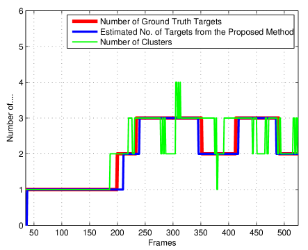
Figure 7: The graph shows the actual number of targets, estimated number of targets by using the proposed method and the number of clusters as a function of video frames for sequence “seq45-3p-1111_cam3_divx_audio” of the AV16.3 dataset.

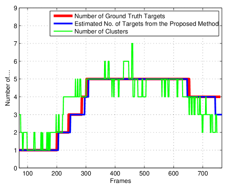
Figure 8: The graph shows the actual number of targets, estimated number of targets by using the proposed method and the number of clusters as a function of video frames for sequence “ThreePastShop2cor” of the CAVIAR dataset.

It is apparent from Figs. 7 and 8 that the number of targets does not always match the number of clusters and hence it is difficult to train the system to estimate the number of targets on the basis of the number of clusters. In the proposed algorithm, instead of using the number of clusters we have exploited the size and location of clusters to estimate the number of targets on all the sequences. This leads to accurate estimation of the number of targets and is demonstrated on Figs. 7 and 8 for two different data sets and in Figs. 9, 10 and 11.

VI-E Tracking Results

A minimum mean square error (MMSE) particle filter is used to estimate the states of the multiple targets. When a new target enters the room, the algorithm automatically initializes it with the help of the data association results by using the mean value of the cluster assigned to that target. Similarly, the algorithm removes the target which leaves the room. The particle size $N_{s}$ is chosen to be equal to $60$ and the number $S$ of social links are updated at every time step. Table I shows the values of the other parameters used in the social force model. The prediction step is performed by the social force model, described in Section II-A.

TABLE I: Parameters of social force model

Symbol	Definition	Value
$b$	Boundary of social force in metres	3m
$r_{i}$	Radius of target’s influence in metres	0.2m
$m$	Mass of target	80kg
$f_{a}$	Magnitude of attractive force	500N
$f_{r}$	Magnitude of repulsive force	500N
$\Delta t$	Time interval	${1}/{25}$

The tracking results for a few selected frames from AV16.3, CAVIAR and PETS2006 datasets are given in Figs. 9, 10 and 11 respectively. Blue, red, green, magenta and cyan ellipses represent first, second, third, fourth and fifth targets, respectively. Fig. 9 shows that the algorithm has successfully initialized new targets in frames $225$ and $278$. In frame $278$ it can be seen that the algorithm can cope with the occlusions between target $1$ and target $2$. Frame $288$ shows that the tracker keeps tracking all targets even when they are very close to each other. Frames $320$ and $326$ show that the algorithm has successfully handled the occlusion between targets $2$ and $3$. In frame $375$ we can see that target $2$ has left the room and the algorithm has automatically removed its tracker, which is started again when the target has returned back in frame $420$. Success in dealing with occlusions between targets $3$ and $1$ can be seen in frames $389$ and $405$.

$\begin{array}[]{c@{\hspace{0.35in}}c@{\hspace{0.35in}}c@{\hspace{0.35in}}c@{\hspace{0.35in}}c}\includegraphics[width=72.26999pt]{fig4a.pdf}\hfil\hskip 25.29494pt&\includegraphics[width=72.26999pt]{fig4b.pdf}\hfil\hskip 25.29494pt&\includegraphics[width=72.26999pt]{fig4c.pdf}\hfil\hskip 25.29494pt&\includegraphics[width=72.26999pt]{fig4d.pdf}\hfil\hskip 25.29494pt&\includegraphics[width=72.26999pt]{fig4e.pdf}\\ \mbox{(a) Frame 124}\hfil\hskip 25.29494pt&\mbox{(b) Frame 225}\hfil\hskip 25.29494pt&\mbox{(c) Frame 278}\hfil\hskip 25.29494pt&\mbox{(d) Frame 288}\hfil\hskip 25.29494pt&\mbox{(e) Frame 320}\\[8.5359pt] \end{array}$ $\begin{array}[]{c@{\hspace{0.35in}}c@{\hspace{0.35in}}c@{\hspace{0.35in}}c@{\hspace{0.35in}}c}\includegraphics[width=72.26999pt]{fig4f.pdf}\hfil\hskip 25.29494pt&\includegraphics[width=72.26999pt]{fig4g-imp.pdf}\hfil\hskip 25.29494pt&\includegraphics[width=72.26999pt]{fig4h-imp.pdf}\hfil\hskip 25.29494pt&\includegraphics[width=72.26999pt]{fig4i-imp.pdf}\hfil\hskip 25.29494pt&\includegraphics[width=72.26999pt]{fig4j-imp.pdf}\\ \mbox{(f) Frame 326}\hfil\hskip 25.29494pt&\mbox{(g) Frame 375}\hfil\hskip 25.29494pt&\mbox{(h) Frame 389}\hfil\hskip 25.29494pt&\mbox{(i) Frame 405}\hfil\hskip 25.29494pt&\mbox{(j) Frame 420}\end{array}$

Figure 9: Tracking results for certain frames of sequence “seq45-3p-1111_cam3_divx_audio” of the AV16.3 dataset with a variable number of targets while handling complex occlusions. (a) tracking of one target, (b), (c) and (j) show that the algorithm successfully initializes the new tracker, (g) shows that the tracker is deleted when the target leaves the room, (c)-(i) show successful occlusion handling.

$\begin{array}[]{c@{\hspace{0.35in}}c@{\hspace{0.35in}}c@{\hspace{0.35in}}c@{\hspace{0.35in}}c}\includegraphics[width=72.26999pt]{t153.pdf}\hfil\hskip 25.29494pt&\includegraphics[width=72.26999pt]{t332.pdf}\hfil\hskip 25.29494pt&\includegraphics[width=72.26999pt]{t377.pdf}\hfil\hskip 25.29494pt&\includegraphics[width=72.26999pt]{t409.pdf}\hfil\hskip 25.29494pt&\includegraphics[width=72.26999pt]{t440.pdf}\\ \mbox{(a) Frame 152}\hfil\hskip 25.29494pt&\mbox{(b) Frame 334}\hfil\hskip 25.29494pt&\mbox{(c) Frame 379}\hfil\hskip 25.29494pt&\mbox{(d) Frame 409}\hfil\hskip 25.29494pt&\mbox{(e) Frame 440}\end{array}$

$\begin{array}[]{c@{\hspace{0.35in}}c@{\hspace{0.35in}}c@{\hspace{0.35in}}c@{\hspace{0.35in}}c}\includegraphics[width=72.26999pt]{t452.pdf}\hfil\hskip 25.29494pt&\includegraphics[width=72.26999pt]{t475.pdf}\hfil\hskip 25.29494pt&\includegraphics[width=72.26999pt]{t497.pdf}\hfil\hskip 25.29494pt&\includegraphics[width=72.26999pt]{t524.pdf}\hfil\hskip 25.29494pt&\includegraphics[width=72.26999pt]{t572.pdf}\\ \mbox{(f) Frame 452}\hfil\hskip 25.29494pt&\mbox{(g) Frame 476}\hfil\hskip 25.29494pt&\mbox{(h) Frame 497}\hfil\hskip 25.29494pt&\mbox{(i) Frame 524}\hfil\hskip 25.29494pt&\mbox{(j) Frame 572}\end{array}$

Figure 10: Tracking results for certain frames of sequence “ThreePastShop2cor” of the CAVIAR dataset : the proposed tracking algorithm can successfully track a variable number of targets while handling complex occlusions.

$\begin{array}[]{c@{\hspace{0.35in}}c@{\hspace{0.35in}}c@{\hspace{0.35in}}c@{\hspace{0.35in}}c}\includegraphics[width=72.26999pt]{o85.pdf}\hfil\hskip 25.29494pt&\includegraphics[width=72.26999pt]{o273.pdf}\hfil\hskip 25.29494pt&\includegraphics[width=72.26999pt]{o292.pdf}\hfil\hskip 25.29494pt&\includegraphics[width=72.26999pt]{o310.pdf}\hfil\hskip 25.29494pt&\includegraphics[width=72.26999pt]{o327.pdf}\\ \mbox{(a) Frame 85}\hfil\hskip 25.29494pt&\mbox{(b) Frame 273}\hfil\hskip 25.29494pt&\mbox{(c) Frame 292}\hfil\hskip 25.29494pt&\mbox{(d) Frame 310}\hfil\hskip 25.29494pt&\mbox{(e) Frame 327}\end{array}$

$\begin{array}[]{c@{\hspace{0.35in}}c@{\hspace{0.35in}}c@{\hspace{0.35in}}c@{\hspace{0.35in}}c}\includegraphics[width=72.26999pt]{o359.pdf}\hfil\hskip 25.29494pt&\includegraphics[width=72.26999pt]{o379.pdf}\hfil\hskip 25.29494pt&\includegraphics[width=72.26999pt]{o996.pdf}\hfil\hskip 25.29494pt&\includegraphics[width=72.26999pt]{o1026.pdf}\hfil\hskip 25.29494pt&\includegraphics[width=72.26999pt]{o1038.pdf}\\ \mbox{(f) Frame 359}\hfil\hskip 25.29494pt&\mbox{(g) Frame 379}\hfil\hskip 25.29494pt&\mbox{(h) Frame 996}\hfil\hskip 25.29494pt&\mbox{(i) Frame 1026}\hfil\hskip 25.29494pt&\mbox{(j) Frame 1038}\end{array}$

Figure 11: Tracking results for certain frames of sequence “S1-T1-C” of the PETS2006 dataset: the proposed tracking algorithm can successfully track a variable number of targets while handling complex occlusions.

Results in Fig. 10 demonstrate that new target appearing in frame $334$ is initialized. In frame $476$ it can be seen that the tracker has solved the occlusion between target three and four. Similarly, frames $524$ and $572$ show that the tracker copes with occlusion between target three and five. A similar behavior is also observed in Fig. 11.

VI-E1 CLEAR MOT matrices

The tracking performance of the proposed algorithm is measured based on two different performance measures: CLEAR multiple object tracking (MOT) matrices [37] and OSPAMT [38]. The performance is compared with the methods proposed in [4], [1] and [35].

The CLEAR MOT measure includes the multiple object tracking precision (MOTP) matrix, miss detection rate, false positive rate and mismatch rate.

Let ${\bf G}_{k}=[({\bf g}_{k}^{1})^{T},\cdots,({\bf g}_{k}^{i})^{T},\cdots,({\bf g}_{k}^{N})^{T}]^{T}$ be the ground truth at time $k\in[k_{s},k_{e}]$, where $k_{s}$ and $k_{e}$ are respectively the starting and ending points of the observation interval. Each ground truth vector component ${\bf g}_{k}^{i}=({\bf{p}}_{k}^{i},{I}_{i})$ contains the actual position and identity of the target $i$. Similarly, ${\bf O}_{k}=[({\bf o}_{k}^{1})^{T},\cdots,({\bf o}_{k}^{i})^{T},\cdots,({\bf o}_{k}^{N})^{T}]^{T}$ represents the output of the tracking algorithm at time $k$, where each ${\bf o}_{k}^{i}=({\hat{\bf{p}}}_{k}^{i},\hat{{I}}_{i})$ represents the estimated location vector and identity variable of target $i$. At every time $k$ the error is defined as:

• Missed detections corresponding to the number of missed targets, calculated based on the difference between the ground truth and the estimates from the developed technique.

• Mismatch corresponding to the number of targets which have given a wrong identity.

• False positives corresponding to the estimated target locations which are not associated with any of the targets.

The threshold is set at $45cm$, which is the distance between the estimated position of a target and its ground truth beyond which it is considered as a missed detection.

If we assume that ${m}_{k}$, ${mme}_{k}$, ${fp}_{k}$ and ${gt}_{k}$ are respectively the total number of missed detections, mismatches, false positives and ground truths at time $k$, the errors are calculated as [37]

$$\overline{m}=\frac{\sum_{k}{m}_{k}}{\sum_{k}{gt}_{k}},\overline{mme}=\frac{\sum_{k}{mme}_{k}}{\sum_{k}{gt}_{k}},\overline{fp}=\frac{\sum_{k}{fp}_{k}}{\sum_{k}{gt}_{k}}.$$ (72)

The precision is calculated as [37]

$$MOTP=\frac{\sum_{k,i}{d}_{i,k}}{\sum_{k,i}{c}_{k}},$$ (73)

where ${d}_{i,k}$ is the distance between the estimated location and the ground truth location of target $i$ and ${c}_{k}$ is the total number of matches found at time step $k$. Table II presents the performance result of the proposed algorithm and the tracking algorithms proposed in [4], [1] and [35]. The performance results are obtained by using $45$ sequences from AV16.3, CAVIAR and PETS2006 datasets. All three datasets have different environments and backgrounds.

TABLE II: Comparison of performance of the proposed tracking algorithm with the approach of [4], [1] and [35]

Method	$\overline{m}(\%)$	$\overline{mme}(\%)$	$\overline{fp}(\%)$
Tracking algorithm [1]	6.41	9.32	3.92
Tracking algorithm [35]	9.38	5.15	5.08
Tracking algorithm [4]	5.41	4.57	1.95
Proposed algorithm	5.04	1.31	0.33

The results show that the proposed algorithm has significantly improved performance compared with other techniques [4], [1] and [35]. Table II shows that there is a significant reduction in missed detections, mismatches and false positives. The reduction in the missed detections is mainly due to the proposed clustering based approach along with the new social force model based estimation technique. A simple particle filter based algorithm without any interaction model proposed by [35] shows the worst results mainly due to the highest number of mismatches. The algorithm proposed in [1] shows better results because of a better interaction model. However, the number of missed detections, mismatches and false positives are higher than that of [4]. This is because [1] does not propose a solution when two targets partially occlude each other or appear again after full occlusion. The technique proposed in [4] gives improved results due to the clustering and the JPDAF however fails when targets reappear after occlusion. This is due to the fact that only location information is used for data association and a simple constant velocity model is used for state prediction. Our proposed algorithm improves the tracking accuracy by reducing the number of missed detections, mismatches and false positives. Reduction in the number of missed detections is mainly due to the proposed particle filter based force model for particles predictions, while the proposed data association technique reduces the chances of mismatches. This improvement is thanks to the utilization of both feature information of targets along with their locations together with the location of clusters.

There is a significant $3.26\%$ reduction in the wrong identifications which has improved the overall accuracy of the tracker. Average precision results for the video sequences from AV16.3, CAVIAR and PETS2006 data sets are shown in Table III.

TABLE III: Comparison of precision of the proposed tracking algorithm with the approach of [4], [1] and [35]

Method	Dataset	MOTP(cm)
	AV16.3	9.07
Tracking algorithm [1]	CAVIAR	11.15
	PETS2006	11.02
	AV16.3	7.12
Tracking algorithm [35]	CAVIAR	9.45
	PETS2006	8.99
	AV16.3	5.85
Tracking algorithm [4]	CAVIAR	7.13
	PETS2006	7.01
	AV16.3	3.97.
Proposed algorithm	CAVIAR	5.52
	PETS2006	5.13

Precision plots for two video sequences against the video frame are shown in Fig. 12. Results show that the MOTP remains less than $4$cm for most of the frames. It increases to $12$cm for the frames where occlusions occur but it again drops when targets emerge from occlusion.

$\begin{array}[]{c@{\hspace{0.32in}}c}\includegraphics[width=216.81pt]{motp1.pdf}\hfil\hskip 23.12692pt\\ \small{\mbox{(a)}}\hfil\hskip 23.12692pt\end{array}$ $\begin{array}[]{c@{\hspace{0.32in}}c}\includegraphics[width=216.81pt]{motp2.pdf}\hfil\hskip 23.12692pt\\ \small\small{\mbox{(b)}}\hfil\hskip 23.12692pt\end{array}$ $\begin{array}[]{c@{\hspace{0.32in}}c}\includegraphics[width=216.81pt]{motp3.pdf}\hfil\hskip 23.12692pt\\ \small\small{\mbox{(c)}}\hfil\hskip 23.12692pt\end{array}$

Figure 12: Precision plot against the video frames of sequences: (a) “seq45-3p-1111_cam3_divx_audio” of the AV16.3 dataset (b)“ThreePastShop2cor” of the CAVIAR dataset (c) “S1-T1-C” of the PETS2006 dataset

VI-E2 OSPAMT

A new performance metric, optimal subpattern assignment metric for multiple tracks (OSPAMT) [38] is also used to evaluate the performance of the proposed technique and approach of [4]. The OSPAMT metric calculates the localization distance $\mathcal{D}_{k}^{Loc}(\omega,\omega^{\prime})$ between a set of true tracks $\omega$ and a set of estimated tracks $\omega^{\prime}$ at time step $k$ as follows

$$\mathcal{D}^{Loc}_{k}(\omega,\omega^{\prime})=\biggr{[}\frac{1}{n_{t}}\sum_{i=1}^{|\omega|}d_{k}(\tau_{i}^{\omega},\omega^{\prime})\biggr{]}^{1/p},$$ (74)

where $n_{t}=\max\{n_{t}^{\omega},n_{t}^{\omega^{\prime}}\}$ and $n_{t}^{\omega}$ and $n_{t}^{\omega^{\prime}}$ are the number of targets in true and estimated set of tracks, respectively, at time step $k$. The distance $d_{t}(\tau_{i}^{\omega},\omega^{\prime})$ is between the $i^{th}$ true track and the set of estimated tracks $\omega^{\prime}$, complete explanation of which can be found in Section IV of [38]. The distance $\mathcal{D}^{Card}_{k}(\omega,\omega^{\prime})$ at time index $k$ is calculated as

$$\mathcal{D}^{Card}_{k}(\omega,\omega^{\prime})=\biggr{[}\frac{1}{n_{t}}\mathcal{S}_{k}\biggr{]}^{1/p},$$ (75)

where $\mathcal{S}_{t}$ is defined as follows

$$\begin{split}\mathcal{S}_{k}=\sum_{i=1}^{|\omega|}|\tau_{i}^{\omega}(k)|\max\{\bar{n}_{k,i}^{\lambda}-1,0\}(\Delta^{p}+c^{p})+\\ c^{p}(n_{k}-\sum_{i=1}^{|\omega|}\bar{n}_{k,i}^{\lambda}|\tau_{i}^{\omega}(k)|),\end{split}$$ (76)

where $\bar{n}_{k,i}^{\lambda}$ is the number of targets at time $k$ in $\omega^{\prime}$ assigned to target $i$ in $\omega$, $\lambda$ represents an assignment between tracks in $\omega^{\prime}$ and the tracks in $\omega$, $\Delta$ is the assignment parameter, $c$ is the cutoff parameter and $p=2$. Details about all these parameters and the OSPAMT metric can be found in [38]. For results in Figures 13 and 14 we have used $c=80$ and $\Delta=10$. Note that $\mathcal{D}^{Card}_{k}(\omega,\omega^{\prime})$ is basically a distance between the objects. Figures 13 and 14 show the OSPAMT distances, (75) and (76), respectively, plotted against the video frame index. Figure 13 shows low localization errors compared to the technique proposed in [4]. Figure 14 indicates a peak dynamic error when a new target enters the field of view which is between frame numbers $63$ and $65$.

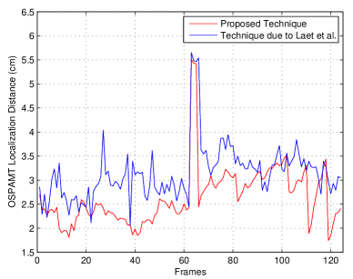
Figure 13: OSPAMT localization distance plot against the video frames of sequence “ThreePastShop2cor” of the CAVIAR dataset

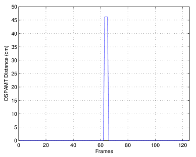
Figure 14: OSPAMT distance plot against the video frames of sequence “ThreePastShop2cor” of the CAVIAR dataset.

VI-F Computational complexity

A variable measurement size technique reduces significantly the computational complexity. The measurement size is increased or decreased on the basis of the distance between the targets. Downsampling of foreground pixels is performed when the distance between targets becomes $80$cm or less. The decrease in the measurement size reduces the time and number of iterations for reaching clustering convergence which results in improved computational complexity. This is shown in Table IV with the help of a few selected frames from sequence “seq45-3p-1111_cam3_divx_audio” of the AV16.3 dataset.

TABLE IV: Comparison of convergence iterations for different measurement sizes

Frame	Minimum	Measurement Size		Convergence Iterations
No.	Distance	Original	Reduced	Original	Reduced
210	227.33	11439	1255	193	15
218	201.01	14496	1614	389	20
221	186.85	15887	1780	282	25
225	159.64	17792	1966	279	29
228	137.60	17819	1964	334	40

Table IV also demonstrates that the proposed technique reduces the number of iterations needed for achieving convergence. The reduction in the number of iterations for convergence improves the run-time of the tracking algorithm. The average run-time (calculated using $45$ video sequences from three datasets) of the proposed algorithm due to the reduction in number of iterations is $0.587$ seconds per frame, as compared to the run-time without measurement reduction which is $2.611$ seconds per frame. The run-time of the approach of [4] is $1.417$ seconds per frame. This run-time comparison is made by implementing the algorithms on MATLAB (version R2012a) with a $3.2$GHz I5 processor.

VI-G Summary

Successful background subtraction is achieved with the help of the codebook background subtraction technique and the results are shown in Figs. 1-3. Grouping foreground pixels into clusters with the help of the proposed variational Bayesian technique is presented in Figs. 4-6. Tracking results are shown in Figs. 9-11. The variational Bayesian clustering improves the overall tracking results especially during close inter-target occlusions. The JPDAF based technique proposed in [4] does not always assign the appropriate clusters to the targets and hence results in tracking failures while solving the complex occlusions.

The graphical results shown in Figs. 7 and 8 indicate that estimating the number of targets on the basis of the number of clusters does not produce accurate results because the number of clusters does not always vary with the number of targets. Figs. 9, 10 and 11 show that accurate target number estimation results are achieved by the proposed technique thanks to exploiting the sizes and locations of clusters, and the estimated state of the targets at the previous time step.

The results in Tables II and III confirm that the overall performance of the proposed tracking algorithm results in an improvement as compared with the recently proposed techniques [4], [1] and [35].

VII Discussion

The quality of the clustering results influences the proposed data association technique. We initialize the clusters on the basis of the estimated locations of targets and by taking into account merging and splitting of targets. The motion of people is predicted with the social force model. This yields accurate clustering results in scenarios where one cluster contains regions of multiple targets. Therefore, the proposed data association technique performs well even during close interactions of targets. It associates multiple clusters to targets with the correct proportion of probability. These association results help in achieving highly accurate tracking of multiple targets even during their close interactions and partial occlusions. The extensive evaluation of the proposed technique on $45$ sequences from three very different datasets validates the tracking accuracy of the proposed algorithm in such scenarios.

A further improvement in accuracy of cluster-to-target association can be achieved by calculating joint associations between multiple clusters. A several-to-one or several-to-several correspondence strategy can be adopted. However, for these strategies the association problem is combinatorial and complexity may become intractable because it will grow geometrically. The cluster-to-target association can also be improved by considering the regions of multiple targets in a cluster as unique identities and associating those regions to respective targets [27].

VIII Conclusions

A learned variational Bayesian clustering and social force model algorithm has been presented for multi-target tracking by using multiple measurements originating from a target. An improved data association technique is developed that exploits the clustering information to solve complex inter-target occlusions. The algorithm accurately and robustly handles a variable number of targets. Its is compared extensively with recent techniques [1], [4] and [35].

Acknowledgment: We are grateful to the support from the UK EPSRC via grant EP/K021516/1, Bayesian Tracking and Reasoning over Time (BTaRoT). We greatly appreciate the constructive comments of the Associate Editor and anonymous reviewers helping us to improve this paper.

Appendices

VIII-A Derivation of equation (45)

The presented derivation is for time index $k$ and for simplicity we omit the index $k$ from the equations. According to (42) we can write

$$\ln\mathcal{Q}^{*}({\bf B})=E_{{\bf C},\boldsymbol{\mu},\boldsymbol{\Sigma}}[\ln p({\tilde{\bf y}},{\bf B},{\bf C},\boldsymbol{\mu},\boldsymbol{\Sigma})]+Const.$$ (77)

and using the decomposition of equation (37) we have

$$\begin{split}\ln\mathcal{Q}^{*}({\bf B})=E_{{\bf C},\boldsymbol{\mu},\boldsymbol{\Sigma}}[\ln p({\tilde{\bf y}}|{\bf B},{\boldsymbol{\mu}},{\bf\Sigma})+\ln p({\bf B}|{\bf C})+\\ \ln p({\bf C})+\ln p({\boldsymbol{\mu}}|{\bf\Sigma})+\ln p({\bf\Sigma})]+Const.\end{split}$$ (78)

The optimal distribution over ${\bf B}$ is calculated by considering different forms of $q({\bf B})$ and by keeping the remaining terms constant. Therefore, quantities not depending on ${\bf B}$ will merge into the constant and we can write equation (78) as

$$\begin{split}\ln\mathcal{Q}^{*}({\bf B})=E_{{\bf C},\boldsymbol{\mu},\boldsymbol{\Sigma}}[\ln p({\tilde{\bf y}}|{\bf B},{\boldsymbol{\mu}},{\bf\Sigma})+\ln p({\bf B}|{\bf C})]+Const.\\ =E_{\boldsymbol{\mu},\boldsymbol{\Sigma}}[\ln p({\tilde{\bf y}}|{\bf B},{\boldsymbol{\mu}},{\bf\Sigma})]+E_{{\bf C}}[\ln p({\bf B}|{\bf C})]+Const.\end{split}$$ (79)

By using equations (32) and (33) we can write

$$\begin{split}\ln\mathcal{Q}^{*}({\bf B})=E_{\boldsymbol{\mu},\boldsymbol{\Sigma}}\biggr{[}\ln\prod_{j=1}^{M}\prod_{q=1}^{\kappa}\mathcal{N}{({\tilde{\bf y}}^{j}|{\boldsymbol{\mu}}^{q},{\bf\Sigma}^{q})}^{b^{j,q}}\biggr{]}+~{}~{}~{}~{}~{}~{}~{}~{}\\ E_{{\bf C}}\biggr{[}\ln\prod_{j=1}^{M}\prod_{q=1}^{\kappa}{(C^{q})}^{b^{j,q}}\biggr{]}+Const.\\ =\sum_{j=1}^{M}\sum_{q=1}^{\kappa}{b^{j,q}}E_{\boldsymbol{\mu},\boldsymbol{\Sigma}}[\ln\mathcal{N}{({\tilde{\bf y}}^{j}|{\boldsymbol{\mu}}^{q},{\bf\Sigma}^{q})}]+~{}~{}~{}~{}~{}~{}~{}~{}\\ \sum_{j=1}^{M}\sum_{q=1}^{\kappa}{{b^{j,q}E_{{\bf C}}\ln(C^{q})}}+Const.\\ =\sum_{j=1}^{M}\sum_{q=1}^{\kappa}{b^{j,q}}E_{\boldsymbol{\mu},\boldsymbol{\Sigma}}\biggr{[}\ln\biggr{\{}\frac{1}{(2\pi)^{D/2}|\boldsymbol{\Sigma}^{q}|^{1/2}}~{}~{}~{}~{}~{}~{}~{}~{}~{}\\ \exp\biggr{(}-\frac{1}{2}({\tilde{\bf y}}^{j}-{\boldsymbol{\mu}}^{q})^{T}(\boldsymbol{\Sigma}^{q})^{-1}({\tilde{\bf y}}^{j}-{\boldsymbol{\mu}}^{q})\biggr{)}\biggr{\}}\biggr{]}+\\ \sum_{j=1}^{M}\sum_{q=1}^{\kappa}{{b^{j,q}E_{{\bf C}}\ln(C^{q})}}+Const.\\ =\biggr{[}\sum_{j=1}^{M}\sum_{q=1}^{\kappa}{b^{j,q}}E_{\boldsymbol{\mu},\boldsymbol{\Sigma}}\biggr{[}-\frac{D}{2}\ln{(2\pi)}-\frac{1}{2}\ln|\boldsymbol{\Sigma}^{q}|~{}~{}~{}~{}~{}\\ -\frac{1}{2}({\tilde{\bf y}}^{j}-{\boldsymbol{\mu}}^{q})^{T}(\boldsymbol{\Sigma}^{q})^{-1}({\tilde{\bf y}}^{j}-{\boldsymbol{\mu}}^{q})\biggr{]}+\\ {b^{j,q}E_{{\bf C}}\ln(C^{q})}\biggr{]}+Const.\\ =\sum_{j=1}^{M}\sum_{q=1}^{\kappa}{b^{j,q}}\biggr{[}-\frac{D}{2}\ln{(2\pi)}-\frac{1}{2}E_{\boldsymbol{\Sigma}}[\ln|\boldsymbol{\Sigma}^{q}|]~{}~{}~{}~{}~{}~{}~{}\\ -\frac{1}{2}E_{\boldsymbol{\mu},\boldsymbol{\Sigma}}[({\tilde{\bf y}}^{j}-{\boldsymbol{\mu}}^{q})^{T}(\boldsymbol{\Sigma}^{q})^{-1}({\tilde{\bf y}}^{j}-{\boldsymbol{\mu}}^{q})]+\\ E_{{\bf C}}\ln(C^{q})\biggr{]}+Const.\end{split}$$ (80)

Considering that

$$\begin{split}\ln{{\rho}}^{j,q}=-\frac{D}{2}\ln{(2\pi)}-\frac{1}{2}E_{\boldsymbol{\Sigma}}[\ln|\boldsymbol{\Sigma}^{q}|]~{}~{}~{}~{}~{}~{}~{}~{}~{}~{}~{}~{}~{}~{}~{}~{}~{}~{}~{}~{}~{}~{}~{}~{}~{}~{}~{}\\ -\frac{1}{2}E_{\boldsymbol{\mu},\boldsymbol{\Sigma}}[({\tilde{\bf y}}^{j}-{\boldsymbol{\mu}}^{q})^{T}(\boldsymbol{\Sigma}^{q})^{-1}({\tilde{\bf y}}^{j}-{\boldsymbol{\mu}}^{q})]+E_{{\bf C}}\ln(C^{q})\end{split}$$ (81)

we get

$$\begin{split}\ln\mathcal{Q}^{*}({\bf B})=\sum_{j=1}^{M}\sum_{q=1}^{\kappa}{b^{j,q}}\ln{{\rho}}^{j,q}+Const.\\ =\prod_{j=1}^{M}\prod_{q=1}^{\kappa}({{\rho}}^{j,q})^{b^{j,q}}+Const.\end{split}$$ (82)

where according to [32]

$$\begin{split}E_{\boldsymbol{\Sigma}}[\ln|\boldsymbol{\Sigma}^{q}|]=\sum_{\tilde{i}}^{D}{\tilde{\psi}\biggr{(}\frac{\upsilon+1-\tilde{i}}{2}}\biggr{)}+D\ln 2+ln|{\bf W}_{q}|\\ E_{\boldsymbol{\mu},\boldsymbol{\Sigma}}[({\tilde{\bf y}}^{j}-{\boldsymbol{\mu}}^{q})^{T}(\boldsymbol{\Sigma}^{q})^{-1}({\tilde{\bf y}}^{j}-{\boldsymbol{\mu}}^{q})]=D\beta_{q}^{-1}+\upsilon_{q}({\tilde{\bf y}}^{j}-{\bf m}_{q})^{T}\\ {\bf W}_{q}({\tilde{\bf y}}^{j}-{\bf m}_{q})~{}~{}~{}~{}~{}~{}~{}~{}~{}~{}~{}~{}~{}\\ E_{{\bf C}}\ln(C^{q})=\tilde{\psi}(\alpha^{q})-\tilde{\psi}(\tilde{\alpha})~{}~{}~{}~{}~{}~{}~{}~{}~{}~{}~{}~{}~{}~{}~{}~{}~{}~{}~{}~{}~{}~{}~{}~{}~{}~{}~{}~{}~{}~{}~{}\end{split}$$ (83)

where $\tilde{\alpha}=\sum_{q=1}^{\kappa}\alpha^{q}$ and $\tilde{\psi}(\cdot)$ is the digamma function. We can write

$$\mathcal{Q}^{*}({\bf B})\propto\prod_{j=1}^{M}\prod_{q=1}^{\kappa}({{\rho}}^{j,q})^{b^{j,q}}$$ (84)

Requiring that this distribution be normalized,

$${r}^{j,q}=\frac{{\boldsymbol{\rho}}^{j,q}}{\sum_{q=1}^{\kappa}{\boldsymbol{\rho}}^{j,q}},$$ (85)

VIII-B Derivation of equation (48)

Using again equation (41) we can write

$$\ln\mathcal{Q}^{*}({\bf C},{\boldsymbol{\mu}},\boldsymbol{\Sigma})=E_{{\bf B}}[\ln p({\tilde{\bf y}},{\bf B},{\bf C},\boldsymbol{\mu},\boldsymbol{\Sigma})]+Const.$$ (86)

According to the decomposition of equation (37) we have

$$\begin{split}\ln\mathcal{Q}^{*}({\bf C},{\boldsymbol{\mu}},\boldsymbol{\Sigma})=E_{{\bf B}}[\ln p({\tilde{\bf y}}|{\bf B},{\boldsymbol{\mu}},{\bf\Sigma})+\ln p({\bf B}|{\bf C})\\ +\ln p({\bf C})+\ln p({\boldsymbol{\mu}}|{\bf\Sigma})+\ln p({\bf\Sigma})]+Const.\end{split}$$ (87)

$$\begin{split}\ln\mathcal{Q}^{*}({\bf C},{\boldsymbol{\mu}},\boldsymbol{\Sigma})=\ln p({\bf C})+E_{{\bf B}}[\ln p({\bf B}|{\bf C})]+\ln p({\boldsymbol{\mu}}|{\bf\Sigma})+\\ \ln p({\bf\Sigma})+E_{{\bf B}}[\ln p({\tilde{\bf y}}|{\bf B},{\boldsymbol{\mu}},{\bf\Sigma})]+Const.\end{split}$$ (88)

which can also be written as

$$\begin{split}\ln\mathcal{Q}^{*}({\bf C},{\boldsymbol{\mu}},\boldsymbol{\Sigma})=\ln p({\bf C})+E_{{\bf B}}[\ln p({\bf B}|{\bf C})]+\ln p({\boldsymbol{\mu}},{\bf\Sigma})\\ +E_{{\bf B}}[\ln p({\tilde{\bf y}}|{\bf B},{\boldsymbol{\mu}},{\bf\Sigma})]+Const.\end{split}$$ (89)

By using equation (33), we can write the above equation as

$$\begin{split}\ln\mathcal{Q}^{*}({\bf C},{\boldsymbol{\mu}},\boldsymbol{\Sigma})=\ln p({\bf C})+E_{{\bf B}}[\ln p({\bf B}|{\bf C})]+\ln p({\boldsymbol{\mu}},{\bf\Sigma})\\ +E_{{\bf B}}\biggr{[}\ln\prod_{j=1}^{M}\prod_{q=1}^{\kappa}\mathcal{N}{({\tilde{\bf y}}^{j}|{\boldsymbol{\mu}}^{q},{\bf\Sigma}^{q})}^{b^{j,q}}\biggr{]}+Const.\end{split}$$ (90)

Also

$$\begin{split}\ln\mathcal{Q}^{*}({\bf C},{\boldsymbol{\mu}},\boldsymbol{\Sigma})=\ln p({\bf C})+E_{{\bf B}}[\ln p({\bf B}|{\bf C})]+\sum_{q=1}^{\kappa}\ln p({\boldsymbol{\mu}}^{q},{\bf\Sigma}^{q})+\\ \sum_{j=1}^{M}\sum_{q=1}^{\kappa}E_{{\bf B}}[{b^{j,q}}\ln\mathcal{N}{({\tilde{\bf y}}^{j}|{\boldsymbol{\mu}}^{q},{\bf\Sigma}^{q})}]+Const.\end{split}$$ (91)

We know that the right-hand side of this expression decomposes into a sum of terms involving only ${\bf C}$ and the terms only involving $\boldsymbol{\mu}$ and ${\boldsymbol{\Sigma}}$ which implies that $p({\bf C},\boldsymbol{\mu},\boldsymbol{\Sigma})$ factorizes to give $p({\bf C})p(\boldsymbol{\mu},\boldsymbol{\Sigma})$.

$$p({\boldsymbol{\mu}},{\bf\Sigma},{\bf C})=p({\bf C})p({\boldsymbol{\mu}},{\bf\Sigma})$$ (92)

By keeping only those terms of (91) which depend on ${\bf C}$ we get

$$\ln\mathcal{Q}^{*}({\bf C})=\ln p({\bf C})+E_{{\bf B}}[\ln p({\bf B}|{\bf C})]+Const.$$ (93)

From equation (46), we know

$$p({\bf C})=Dir({\bf C}|\alpha_{\circ})=\prod_{q=1}^{\kappa}({\bf C}^{q})^{(\alpha_{\circ}-1)}$$ (94)

and therefore

$$\ln p({\bf C})={(\alpha_{\circ}-1)}\sum_{q=1}^{\kappa}\ln{\bf C}^{q}.$$ (95)

According to equation (43)

$$p({\bf B}|{\bf C})=\prod_{j=1}^{M}\prod_{q=1}^{\kappa}{({\bf C}^{q})}^{b^{j,q}}.$$ (96)

Using equation (95) and (96) in (93) we get

$$\begin{split}\ln\mathcal{Q}^{*}({\bf C})={(\alpha_{\circ}-1)}\sum_{q=1}^{\kappa}\ln{\bf C}^{q}+E_{{\bf B}}\biggr{[}\sum_{j=1}^{M}\sum_{q=1}^{\kappa}{{b^{j,q}}\ln({\bf C}^{q})}\biggr{]}\\ +Const.\end{split}$$ (97)

$$\begin{split}\ln\mathcal{Q}^{*}({\bf C})\!=\!\!\!{(\alpha_{\circ}-1)}\sum_{q=1}^{\kappa}\ln{\bf C}^{q}\!+\!\sum_{j=1}^{M}\sum_{q=1}^{\kappa}{E_{\bf B}[{b^{j,q}}\ln({\bf C}^{q})}]\!\!+\!Const.\end{split}$$ (98)

For the discrete distribution $\mathcal{Q}^{*}({\bf B})$ we have the standard result (a similar representation is shown in equation (10.50) of [32]), and $E_{\bf B}[b^{j,q}]=r^{j,q}$. Therefore

$$\ln\mathcal{Q}^{*}({\bf C})={(\alpha_{\circ}-1)}\sum_{q=1}^{\kappa}\ln{\bf C}^{q}+\sum_{j=1}^{M}\sum_{q=1}^{\kappa}{r^{j,q}}\ln({\bf C}^{q})+Const.$$ (99)

by taking the exponential on both sides

$$\mathcal{Q}^{*}({\bf C})=\prod_{q=1}^{\kappa}({\bf C}^{q})^{(\alpha_{\circ}-1)}\prod_{j=1}^{M}\prod_{q=1}^{\kappa}({\bf C}^{q})^{r^{j,q}}+Const.$$ (100)

$$\mathcal{Q}^{*}({\bf C})=\prod_{q=1}^{\kappa}({\bf C}^{q})^{(\alpha_{\circ}-1)}\prod_{q=1}^{\kappa}({\bf C}^{q})^{\sum_{j=1}^{M}{r^{j,q}}}+Const.$$ (101)

$$\mathcal{Q}^{*}({\bf C})=\prod_{q=1}^{\kappa}({\bf C}^{q})^{(\alpha_{\circ}-1}({\bf C}^{q})^{\sum_{j=1}^{M}{r^{j,q}}}+Const.$$ (102)

Suppose ${\sum_{j=1}^{M}{r^{j,q}}}=N^{q}$, then

$$\mathcal{Q}^{*}({\bf C})=\prod_{q=1}^{\kappa}({\bf C}^{q})^{(\alpha_{\circ}-1)}({\bf C}^{q})^{N^{q}}+Const.$$ (103)

$$\mathcal{Q}^{*}({\bf C})=\prod_{q=1}^{\kappa}({\bf C}^{q})^{(\alpha_{\circ}-1)+{N^{q}}}+Const.$$ (104)

by comparing it with equation (94), $\mathcal{Q}^{*}({\bf C})=Dir({\bf C}|\alpha),$ where $\alpha={(\alpha_{\circ}-1)+{N^{q}}}$.

VIII-C Derivation of equation (52)

Consider again the factorization of $p({\bf C},\boldsymbol{\mu},\boldsymbol{\Sigma})$ to give $p({\bf C}),p(\boldsymbol{\mu},\boldsymbol{\Sigma})$. By keeping only those terms of equation (91) which depend on ${\boldsymbol{\mu}}$ and ${\boldsymbol{\Sigma}}$ we get

$$\begin{split}\ln\mathcal{Q}^{*}({\boldsymbol{\mu}},\boldsymbol{\Sigma})=\sum_{q=1}^{\kappa}\ln p({\boldsymbol{\mu}}^{q},{\bf\Sigma}^{q})+~{}~{}~{}~{}~{}~{}~{}~{}~{}~{}~{}~{}~{}~{}~{}~{}~{}~{}~{}~{}~{}~{}~{}~{}~{}~{}\\ \sum_{j=1}^{M}\sum_{q=1}^{\kappa}E_{{\bf B}}[{b^{j,q}}\ln\mathcal{N}{({\tilde{\bf y}}^{j}|{\boldsymbol{\mu}}^{q},{\bf\Sigma}^{q})}]+Const.\end{split}$$ (105)

According to equation (51)

$$p({\boldsymbol{\mu}},{\bf\Sigma})=\prod_{q=1}^{\kappa}\mathcal{N}({\boldsymbol{\mu}}^{q}|{\bf m}_{\circ},\beta_{\circ}^{-1}{\bf\Sigma}^{q})\mathcal{W}({\bf\Sigma}^{q}|{\bf W}_{\circ},\upsilon_{\circ})$$ (106)

therefore

$$\begin{split}\ln\mathcal{Q}^{*}({\boldsymbol{\mu}},\boldsymbol{\Sigma})=\sum_{q=1}^{\kappa}\ln\mathcal{N}({\boldsymbol{\mu}}^{q}|{\bf m}_{\circ},\beta_{\circ}^{-1}{\bf\Sigma}^{q})+\ln\mathcal{W}({\bf\Sigma}^{q}|{\bf W}_{\circ},\upsilon_{\circ})\\ +\sum_{j=1}^{M}\sum_{q=1}^{\kappa}E_{{\bf B}}[{b^{j,q}}\ln\mathcal{N}{({\tilde{\bf y}}^{j}|{\boldsymbol{\mu}}^{q},{\bf\Sigma}^{q})}]+Const.\end{split}$$ (107)

whereas the Wishart distribution can be defined as

$$\mathcal{W}({\bf\Sigma}^{q}|{\bf W}_{\circ},\upsilon_{\circ})=\frac{({\bf\Sigma}^{q})^{(\upsilon_{\circ}-D-1)}\\ \exp(\frac{-1}{2}T_{r}({\bf W}_{\circ}({\bf\Sigma}^{q})^{-1}))}{2^{\upsilon_{\circ}D/2}|{\bf W}_{\circ}|^{\upsilon_{\circ}/2}T_{D}(\upsilon_{\circ}/2)}$$ (108)

also

$$\begin{split}\mathcal{N}({\boldsymbol{\mu}}^{q}|{\bf m}_{\circ},\beta_{\circ}^{-1}{\bf\Sigma}^{q})=\biggr{[}\ln\biggr{\{}\frac{1}{(2\pi)^{D/2}(\beta_{\circ}^{-1}|\boldsymbol{\Sigma}^{q}|)^{1/2}}\\ \exp\biggr{(}-\frac{1}{2}({\boldsymbol{\mu}}^{q}-{\bf m}_{\circ})^{T}\beta_{\circ}\boldsymbol{\Sigma}_{q}^{-1}({\boldsymbol{\mu}}^{q}-{\bf m}_{\circ})\biggr{)}\biggr{\}}\biggr{]}\end{split}$$ (109)

Using these equations in (107), keeping only the terms which contain $\boldsymbol{\mu}$ and $\boldsymbol{\Sigma}$ we get the final expression for (52) where $\beta_{q},{\bf m}_{q},{\bf W}_{q}$ and $\upsilon_{q}$ are defined in (53)-(57).

Ata-ur-Rehman received the B.Eng. degree in electronic engineering from Air University, Islamabad, Pakistan in 2006. He then joined the University of Engineering and Technology, Lahore, Pakistan, as a Lecturer/Lab Engineer in 2007. He moved to Loughborough University, U.K., in 2009 where he received his M.Sc. degree with distinction in Digital Communication Systems in 2010. He received his Ph.D degree in Signal Processing from Loughborough University, UK in 2014. Since December 2013 he is a PDRA at the Department of ACSE, The University of Sheffield. His main area of research is multi-target tracking.

Mohsen Naqvi (S’06-M’09-SM’14) received Ph.D. degree in Signal Processing from Loughborough University, UK in 2009. Where he was a PDRA on the EPSRC UK funded projects and REF Lecturer from July 2009 to July 2015. Dr Naqvi is a Lecturer in Signal and Information Processing at the School of Electrical and Electronic Engineering, Newcastle University, UK and Fellow of the Higher Education Academy. His research interests include multimodal processing for human behavior analysis, multi-target tracking and source separation, all for machine learning.

Lyudmila Mihaylova (M’98, SM’2008) is Associate Professor (Reader in Advanced Signal Processing and Control) at the Department of Automatic Control and Systems Engineering at the University of Sheffield, United Kingdom. Her research is in the areas of machine learning and autonomous systems with various applications such as navigation, surveillance and sensor network systems. Dr Mihaylova is an Associate Editor of the IEEE Transactions on Aerospace and Electronic Systems and of the Elsevier Signal Processing Journal.

Jonathon A. Chambers (S’83-M’90-SM’98-F’11) received the Ph.D. and D.Sc. degrees in signal processing from the Imperial College of Science, Technology and Medicine (Imperial College London), London, U.K., in 1990 and 2014, respectively. He is a Professor of signal and information processing within the School of Electrical and Electronic Engineering, Newcastle University, U.K., and a Fellow of the Royal Academy of Engineering, U.K.. He has also served as an Associate Editor for the IEEE TRANSACTIONS ON SIGNAL PROCESSING over the periods 1997-1999, 2004-2007, and as a Senior Area Editor 2011-15.

References

• [1] Z. Khan, T. Balch, and F. Dellaert, “MCMC-Based particle filtering for tracking a variable number of interacting targets,” IEEE Trans. Pattern Analysis and Machine Intelligence, vol. 27, no. 11, pp. 1805–1819, 2005.
• [2] B. Ristic, S. Arulampalam, and N. Gordon, Beyond the Kalman Filter: Particle Filter for Tracking Applications.   Boston—London: Artech House Publishers, 2004.
• [3] S. M. Naqvi, M. Yu, and J. A. Chambers, “A multimodal approach to blind source separation of moving sources,” IEEE J. Selected Topics in Signal Processing, vol. 4, no. 5, pp. 895–910, 2010.
• [4] T. D. Laet, H. Bruyninckx, and J. D. Schutter, “Shape-based online multi-target tracking and detection for targets causing multiple measurements: Variational Bayesian clustering and lossless data association,” IEEE Trans. Pattern Analysis and Machine Intelligence, vol. 33, pp. 2477–2491, 2011.
• [5] M. Montemerlo, W. Whittaker, and S. Thrun, “Particle filters for simultaneous mobile robot localization and people-tracking,” in Proc. IEEE Int. Conf. Robotics and Automation, 2002, pp. 695–701.
• [6] S. Velipasalar and W. Wolf, “Multiple object tracking and occlusion handling by information exchange between uncalibrated cameras,” in Proc. IEEE Int. Conf. Image Processing, vol. 2, 2005, pp. 418–421.
• [7] T. Zhao and R. Nevatia, “Tracking multiple humans in crowded environment,” in Proc. IEEE Computer Society Conf. Computer Vision and Pattern Recognition, vol. 2, 2004, pp. 406–413.
• [8] A. M. Elgammal, R. Duraiswami, and L. S. Davis, “Efficient non-parametric adaptive color modeling using fast Gauss transform,” in Proc. IEEE Conf. Computer Vision Pattern Recognition, vol. 2, 2001, pp. 563–570.
• [9] P. Brasnett, L. Mihaylova, D. Bull, and N. Canagarajah, “Sequential Monte Carlo tracking by fusing multiple cues in video sequences,” Image and Vision Computing, vol. 25, no. 8, pp. 1217–1227, 2007.
• [10] J. Vermaak, S. J. Godsill, and P. Perez, “Monte Carlo filtering for multi-target tracking and data association,” IEEE Trans. Aerospace and Electronic systems, vol. 41, pp. 309–332, 2005.
• [11] S. M. Naqvi, W. Wang, M. S. Khan, M. Barnard, and J. A. Chambers, “Multimodal (audio-visual) source separation exploiting multi-speaker tracking, robust beamforming, and time-frequency masking,” IET Signal Processing, vol. 6, pp. 466–477, 2012.
• [12] K. Nummiaro, E. Koller-Meier, and L. V. Gool, “An adaptive color based particle filter,” Image and Vision Computing, vol. 21, no. 1, pp. 99–110, 2003.
• [13] B. Habtemariam, R. Tharmarasa, T. Thayaparan, M. Mallick, and T. Kirubarajan, “A multiple-detection joint probabilistic data association filter,” IEEE J. Selected Topics in Signal Processing, vol. 7, no. 3, pp. 461–471, 2013.
• [14] H. Benoudnine, M. Keche, A. Ouamri, and M. S. Woolfson, “New efficient schemes for adaptive selection of the update time in the IMM-PDAF ,” IEEE Trans. Aerospace and Electronic Systems, vol. 48, no. 1, pp. 197–214, 2012.
• [15] S. K. Pang, J. Li, and S. J. Godsill, “Detection and tracking of coordinated groups,” IEEE Trans. Aerospace and Electronic Systems, vol. 47, no. 1, pp. 472–502, 2011.
• [16] S. Ali, K. Nishino, D. Manocha, and M. Shah, Modeling, Simulation and Visual Analysis of Crowds.   Springer, 2013.
• [17] D. Helbing and P. Molnár, “Social force model for pedestrian dynamics,” Physical Review E, vol. 51, pp. 4282–4286, 1995.
• [18] R. Mazzon and A. Cavallaro, “Multi-camera tracking using a multi-goal social force model,” Neurocomputing, vol. 100, pp. 41–50, 2013.
• [19] S. Pellegrini, A. Ess, K. Schindler, and L. V. Gool, “You’ll never walk alone: Modeling social behavior for multi-target tracking,” in Proc. IEEE Int. Conf. Computer Vision, 2009, pp. 261–268.
• [20] F. Septier, S. K. Pang, A. Carmi, and S. Godsill, “On MCMC based particle methods for Bayesian filtering: application to multi-target tracking,” in Proc. IEEE Int. Workshop on Computational Advances in Multi-sensor Adaptive Processing, 2009, pp. 360–363.
• [21] R. P. S. Mahler, Statistical Multisource-Multitarget Information Fusion.   Artech House, 2007.
• [22] B. Ristic, J. Sherrah, and Á. F. García-Fernández, “Performance evaluation of random set based pedestrian tracking algorithms,” in Proc. Intelligent Sensors, Sensor Networks and Information Processing, 2013.
• [23] M. S. Arulampalam, S. Maskell, N. Gordon, and T. Clapp, “A tutorial on particle filters for online nonlinear/non-Gaussian Bayesian tracking,” IEEE Trans. Signal Processing, vol. 50, no. 2, pp. 174–188, 2002.
• [24] K. Kim, T. Chalidabhongse, D. Harwood, and L. Davis, “Real-time foreground-background segmentation using codebook model,” Int. J. Real-Time Imaging, vol. 11, pp. 172–185, 2005.
• [25] X. Yan, I. Kakadiaris, and S. Shah, “Modeling local behavior for predicting social interactions towards human tracking,” Pattern Recognition, vol. 47, no. 4, pp. 1626 – 1641, 2014.
• [26] R. Hartley and A. Zisserman, Multiple View Geometry in Computer Vision.   Cambridge University Press, 2001.
• [27] Y. Ma, Q. Yu, and I. Cohen, “Target tracking with incomplete detection,” Computer Vision and Image Understanding, vol. 113, no. 4, pp. 580 – 587, 2009.
• [28] Y. Bar-Shalom and T. Fortman, Tracking and Data Association.   New York: Academic Press, 1988.
• [29] K. G. Murty, “An algorithm for ranking all the assignments in order of increasing cost,” Operations Research, vol. 16, no. 3, pp. 682–687.
• [30] I. J. Cox, “A review of statistical data association techniques for motion correspondence,” Int. J. Computer Vision, vol. 10, pp. 53–66, 1993.
• [31] A. Bhattacharayya, “On a measure of divergence between two statistical populations defined by their probability distributions,” Bulletin of Calcutta Mathematical Society, vol. 35, pp. 99–110, 1943.
• [32] C. M. Bishop, Pattern Recognition and Machine Learning.   Springer, 2006.
• [33] D. Schulz, W. Burgard, D. Fox, and A. B. Cremers, “People tracking with mobile robots using sample-based joint probabilistic data association filters,” The Int. J. Robotics Research, vol. 22, no. 2, pp. 99 –116, 2003.
• [34] W. Ng, J. Li, S. Godsill, and S. K. Pang, “Multi-target initiation, tracking and termination using Bayesian Monte Carlo methods,” Comput. J., vol. 50, no. 6, pp. 674–693, Nov. 2007.
• [35] J. Czyz, B. Ristic, and B. Macq, “A particle filter for joint detection and tracking of color objects,” Image and Vision Computing, vol. 25, no. 8, pp. 1271 – 1281, 2007.
• [36] M. Yu, A. Rhuma, S. M. Naqvi, L. Wang, and J. A. Chambers, “Posture recognition based fall detection system for monitoring an elderly person in a smart home environment,” IEEE Trans. Information Technology in Biomedicine, vol. 16, pp. 1274–1286, 2012.
• [37] K. Bernardin and R. Stiefelhagen, “Evaluating multiple object tracking performance: The clear mot metrics,” J. Image Video Process., vol. 2008, pp. 1–10, 2008.
• [38] T. Vu and R. Evans, “A new performance metric for multiple target tracking based on optimal subpattern assignment,” in Proc. Int. Conf. Information Fusion, July 2014, pp. 1–8.