Guarantees of Riemannian Optimization for Low Rank Matrix Recovery

Abstract

We establish theoretical recovery guarantees of a family of Riemannian optimization algorithms for low rank matrix recovery, which is about recovering an $m\times n$ rank $r$ matrix from $p<mn$ number of linear measurements. The algorithms are first interpreted as iterative hard thresholding algorithms with subspace projections. Based on this connection, we show that provided the restricted isometry constant $R_{3r}$ of the sensing operator is less than $C_{\kappa}/\sqrt{r}$, the Riemannian gradient descent algorithm and a restarted variant of the Riemannian conjugate gradient algorithm are guaranteed to converge linearly to the underlying rank $r$ matrix if they are initialized by one step hard thresholding. Empirical evaluation shows that the algorithms are able to recover a low rank matrix from nearly the minimum number of measurements necessary.

Keywords. Matrix recovery, low rank matrix manifold, Riemannian optimization, gradient descent and conjugate gradient descent methods, restricted isometry constant

Mathematics Subject Classification. 15A29, 41A29, 65F10, 68Q25, 15A83, 53B21, 90C26, 65K05

1 Introduction

Many applications of interest require acquisition of very high dimensional data which can be prohibitively expensive if no simple structures of the data are known. In contrast, data with an inherent low dimensional structure can be acquired more efficiently by exploring the simplicity of the underlying structure. For instance, in compressed sensing [23, 19, 13], a high dimensional vector of length $n$ with only a few nonzero entries can be encoded by $p<n$ linear measurements, where $p$ is essentially determined by the number of nonzero entries. Moreover, the vector can be reconstructed from the measurements by computationally efficient algorithms. Another natural representation of data is matrix which can be imposed other different simple structures in addition to few nonzero entries. A particularly interesting notion of matrix simplicity is low rank.

Low rank matrices can be used to model datasets from a wide range of applications, such as model reduction [39], pattern recognition [24], and machine learning [4, 5]. In this paper, we are interested in the problem of recovering a low rank matrix from a set of linear measurements. Let $X\in\mathbb{R}^{m\times n}$ and assume $\mbox{rank}(X)=r<\min(m,n)$. Let $\mathcal{A}\left(\cdot\right):\mathbb{R}^{m\times n}\rightarrow\mathbb{R}^{p}$ be a linear map from $m\times n$ matrices to $p$ dimensional vectors of the form

$$\mathcal{A}\left(Z\right)_{\ell}=\left\langle A_{\ell},Z\right\rangle,\quad\ell=1,\cdots,p.$$ (1)

We take $p<mn$ linear measurements of $X$ via $y=\mathcal{A}(X)$. To recover the low rank matrix $X$ from the measurement vector $y$, it is natural to seek the lowest rank matrix consistent with the measurements by solving a rank minimization problem

$$\min\mbox{rank}(Z)\mbox{ subject to }\mathcal{A}(Z)=y.$$ (2)

There are two typical sensing operators. One is dense sensing, where each $A_{\ell}$ is a dense matrix, for example, a Gaussian random matrix. The other one is entry sensing with the sensing matrices $A_{\ell}$ only having one nonzero entry equal to one, which corresponds to measuring the entries of a matrix directly. When a subset of the matrix entries are directly measured, seeking a low rank matrix consistent with the known entries is typically referred to as matrix completion [18]. Recovering a low rank matrix when each sensing matrix is dense is usually referred to as low rank matrix recovery [17]. This paper investigates recovery guarantees of the Riemannian optimization algorithms for low rank matrix recovery.

Notice that (2) is a non-convex optimization problem and computationally intractable. One of the well studied approaches is to replace the rank objective in (2) with its nearest convex relaxation, the nuclear norm of matrices which is the sum of the singular values, and then solve the following nuclear norm minimization problem

$$\min\left\|Z\right\|_{*}\mbox{ subject to }\mathcal{A}(Z)=y.$$ (3)

The equivalence of solutions between (2) and (3) for low rank matrix recovery can be established in terms of the restricted isometry constant of the sensing operator which was first introduced in [20] for compressed sensing and subsequently extended to low rank matrix recovery in [48].

Definition 1.1 (Restricted Isometry Constant (RIC) [48]).

Let $\mathcal{A}(\cdot)$ be a linear operator from $m\times n$ matrices to vectors of length $p$. For any integer $0<r\leq\min(m,n)$, the restricted isometry constant, $R_{r}$, is defined as the smallest number such that

$$\left(1-R_{r}\right)\left\|Z\right\|_{F}^{2}\leq\left\|\mathcal{A}\left(Z\right)\right\|_{2}^{2}\leq\left(1+R_{r}\right)\left\|Z\right\|_{F}^{2}$$ (4)

holds for all the matrices $Z$ of rank at most $r$.

It has been proven that if the RIC of $\mathcal{A}\left(\cdot\right)$ with rank $5r$ is less than a small constant, nuclear norm minization (3) is guaranteed to recover any measured rank $r$ matrix [48]. Furthermore, this condition can be satisfied with overwhelmingly high probability for a large family of random measurement matrices, for example the normalized Gaussian and Bernoulli matrices, provided $p\geq C\cdot(m+n-r)r\log^{\alpha}\left(\max\left(m,n\right)\right)$ for some numerical constants $C>0,~{}\alpha\geq 0$ [48, 17]. However, for the entry sensing operator, it cannot have a small RIC for any $r>0$, and more quantitative and probabilistic sampling complexity has been established for (3) based on the notion of incoherence [18, 21, 47, 28].

Nuclear norm minimization is amenable to detailed analysis [48, 18, 21, 47, 28, 49, 46, 33, 3]. However, finding the solution to (3) by the interior-point methods needs to solve systems of linear equations to compute the Newton direction in each iteration, which limits its applicability for large $m$ and $n$. First-order methods for solving (3) usually invoke the singular value thresholding [11]. Alternative to convex relaxation, there have been many algorithms which are designed to target (2) directly, including iterative hard thresholding [7, 30, 37, 52], alternating minimization [29, 59, 53] , and Riemannian optimization [55, 44, 40, 41, 42, 12]. In this paper, we study a family of Riemannian optimization algorithms on the embedded manifold of rank $r$ matrices. We first establish their connections with iterative hard thresholding algorithms. Then we prove local convergence of the Riemannian gradient descent algorithm in terms of the restricted isometry constant of the sensing operator. As a result, the algorithm is guaranteed to converge linearly to the measured low rank matrix if it is initialized by one step hard thresholding. For the Riemannian conjugate gradient descent algorithm, we introduce a restarted variant for which a similar recovery guarantee can be established while the computational efficiency is maintained.

The rest of this paper is organized as follows. In Sec. 2, we briefly review iterative hard thresholding algorithms for low rank matrix recovery and show their connections with the Riemannian optimization algorithms on the embedded manifold of low rank matrices. Then we present the main results of this paper. In Sec. 3, empirical results are presented, which demonstrate the efficiency of the Riemannian optimization algorithms for matrix recovery. Section 4 presents the proofs of the main results and Sec. 5 concludes the paper with future research directions.

2 Algorithms and Main Results

2.1 Iterative Hard Thresholding and Riemannian Optimization

Iterative hard thresholding is a family of simple yet efficient algorithms for compressed sensing [9, 10, 7, 8] and low rank matrix recovery [7, 30, 37, 52]. The simplest iterative hard thresholding algorithm for matrix recovery is the normalized iterative hard thresholding (NIHT [52], also known as SVP [30] or IHT [26] when the stepsize is fixed), see Alg. 1. NIHT applies the projected gradient descent method to a reformulation of (2)

$$\min_{Z\in\mathbb{R}^{m\times n}}\frac{1}{2}\left\|y-\mathcal{A}\left(Z\right)\right\|_{2}^{2}~{}\mbox{ subject to }~{}\mbox{rank}(Z)=r.$$ (5)

Algorithm 1 Normalized Iterative Hard Thresholding (NIHT [52])

  Initilization: $X_{0}$ and its top $r$ left singular vector space $U_{0}$

  for $l=0,1,\cdots$ do

     1. $G_{l}=\mathcal{A}^{*}\left(y-\mathcal{A}\left(X_{l}\right)\right)$

     2. $\alpha_{l}=\frac{\left\|\mathcal{P}_{U_{l}}\left(G_{l}\right)\right\|_{F}^{2}}{\left\|\mathcal{A}\mathcal{P}_{U_{l}}\left(G_{l}\right)\right\|_{2}^{2}}$

     3. $W_{l}=X_{l}+\alpha_{l}G_{l}$

     4. $X_{l+1}=\mathcal{H}_{r}(W_{l})$

  end for

In each iteration of NIHT, the current estimate $X_{l}$ is updated along the gradient descent direction $G_{l}$ with the locally steepest descent stepsize $\alpha_{l}$ defined as

$$\alpha_{l}:=\operatorname*{arg\,min}_{\alpha}\frac{1}{2}\left\|y-\mathcal{A}\left(X_{l}+\alpha\mathcal{P}_{U_{l}}\left(G_{l}\right)\right)\right\|_{F}^{2},$$ (6)

where $\mathcal{P}_{U_{l}}=U_{l}U_{l}^{*}$ denotes the projection to the left singular vector subspace of $X_{l}$. Then the new estimate $X_{l+1}$ is obtained by thresholding $W_{l}$ to the set of rank $r$ matrices. In Alg. 1, $\mathcal{H}_{r}(\cdot)$ denotes the hard thresholding operator which first computes the singular value decomposition of a matrix and then sets all but the $r$ largest singular values to zero

$$\mathcal{H}_{r}(Z):=U\Sigma_{r}V^{*}\quad\mbox{where}\quad\Sigma_{r}(i,i):=\begin{cases}\Sigma(i,i)&i\leq r\\ 0&i>r.\end{cases}$$ (7)

When there are singular values of $Z$ with multiplicity more than one, $\mathcal{H}_{r}(Z)$ can use any one of the repeated singular values and the corresponding singular vectors. In this case, it still returns the best (though not unique) rank $r$ approximation of $Z$ in the Frobenius norm.

NIHT has been proven to be able to recover a rank $r$ matrix if the RIC of $\mathcal{A}(\cdot)$ satisfies $R_{3r}\leq 1/5$ [52]. Despite the optimal recovery guarantee of NIHT, it suffers from the slow asymptotic convergence rate of the gradient descent method. Other sophisticated variants have been designed to overcome the slow asymptotic convergence rate of NIHT. For example in SVP-Newton [30], a least square subproblem restricted onto the current iterate subspace is solved in each iteration. In [7], a family of conjugate gradient iterative hard thresholding (CGIHT) algorithms have been developed for low rank matrix recovery which combines the fast asymptotic convergence rate of more sophisticated algorithms and the low per iteration complexity of NIHT, see Alg. 2 for the non restarted CGIHT.

Algorithm 2 Conjugate Gradient Iterative Hard Thresholding (CGIHT [7])

  Initilization: $X_{0}$ and its top $r$ left singular vector space $U_{0}$, $P_{-1}=0$

  for $l=0,1,\cdots$ do

     1. $G_{l}=\mathcal{A}^{*}\left(y-\mathcal{A}\left(X_{l}\right)\right)$

     2. $\beta_{l}=-\frac{\left\langle\mathcal{A}\mathcal{P}_{U_{l}}\left(G_{l}\right),\mathcal{A}\mathcal{P}_{U_{l}}\left(P_{l-1}\right)\right\rangle}{\left\|\mathcal{A}\mathcal{P}_{U_{l}}\left(P_{l-1}\right)\right\|_{2}^{2}}$

     3. $P_{l}=G_{l}+\beta_{l}P_{l-1}$

     4. $\alpha_{l}=\frac{\left\langle\mathcal{P}_{U_{l}}\left(G_{l}\right),\mathcal{P}_{U_{l}}\left(P_{l}\right)\right\rangle}{\left\|\mathcal{A}\mathcal{P}_{U_{l}}\left(P_{l}\right)\right\|_{2}^{2}}$

     5. $W_{l}=X_{l}+\alpha_{l}P_{l}$

     6. $X_{l+1}=\mathcal{H}_{r}(W_{l})$

  end for

In each iteration of CGIHT, the current estimate $X_{l}$ is updated along the search direction $P_{l}$ with the locally steepest descent stepsize $\alpha_{l}$ defined in a similar way to (6). The current search direction $P_{l}$ is a linear combination of the gradient descent direction and the previous search direction. The selection of the orthogonalization weight $\beta_{l}$ in Alg. 2 ensures that $P_{l}$ is conjugate orthogonal to the $P_{l-1}$ when restricted to the current subspace determined by $U_{l}$. It has been proven that a projected variant of Alg. 2 has the nearly optimal recovery guarantee based on the RIC of the sensing operator [7].

In NIHT and CGIHT, the current estimate is updated along a line search direction which departs from the manifold of rank $r$ matrices. The singular value decomposition is required in each iteration to project the estimate back onto the rank $r$ matrix manifold. The SVD on a full $m\times n$ matrix is typically needed as the search direction is a global gradient descent or conjugate gradient descent direction which does not belong to any particular low dimensional subspace. The computational complexity of the SVD on an $m\times n$ matrix is $O(n^{3})$ when $m$ is proportional to $n$ which is computationally expensive. However, if the estimate is updated along a search direction in a low dimensional subspace, the intermediate matrix $W_{l}$ may also be a low rank matrix. So it is possible to work on a matrix of size much smaller than $m$ and $n$ when truncating $W_{l}$ to its nearest rank $r$ approximation. The generalized NIHT and CGIHT for low rank matrix recovery [56] are presented in Algs. 3 and 4 respectively, which explore the idea of projecting the search direction onto a low dimensional subspace associated with the current estimate.

Algorithm 3 Riemannian Gradient Descent (RGrad)

  Initilization: $X_{0}$

  for $l=0,1,\cdots$ do

     1. $G_{l}=\mathcal{A}^{*}\left(y-\mathcal{A}\left(X_{l}\right)\right)$

     2. $\alpha_{l}=\frac{\left\|\mathcal{P}_{\mathcal{S}_{l}}\left(G_{l}\right)\right\|_{F}^{2}}{\left\|\mathcal{A}\mathcal{P}_{\mathcal{S}_{l}}\left(G_{l}\right)\right\|_{2}^{2}}$

     3. $W_{l}=X_{l}+\alpha_{l}\mathcal{P}_{\mathcal{S}_{l}}\left(G_{l}\right)$

     4. $X_{l+1}=\mathcal{H}_{r}(W_{l})$

  end for

Algorithm 4 Riemannian Conjugate Gradient Descent (RCG)

  Initilization: $X_{0}$, $\beta_{0}=0$ and $P_{-1}=0$

  for $l=0,1,\cdots$ do

     1. $G_{l}=\mathcal{A}^{*}\left(y-\mathcal{A}\left(X_{l}\right)\right)$

     2. $\beta_{l}=-\frac{\left\langle\mathcal{A}\mathcal{P}_{\mathcal{S}_{l}}\left(G_{l}\right),\mathcal{A}\mathcal{P}_{\mathcal{S}_{l}}\left(P_{l-1}\right)\right\rangle}{\left\|\mathcal{A}\mathcal{P}_{\mathcal{S}_{l}}\left(P_{l-1}\right)\right\|_{2}^{2}}$

     3. $P_{l}=\mathcal{P}_{\mathcal{S}_{l}}\left(G_{l}\right)+\beta_{l}\mathcal{P}_{\mathcal{S}_{l}}\left(P_{l-1}\right)$

     4. $\alpha_{l}=\frac{\left\langle\mathcal{P}_{\mathcal{S}_{l}}\left(G_{l}\right),\mathcal{P}_{\mathcal{S}_{l}}\left(P_{l}\right)\right\rangle}{\left\|\mathcal{A}\mathcal{P}_{\mathcal{S}_{l}}\left(P_{l}\right)\right\|_{2}^{2}}$

     5. $W_{l}=X_{l}+\alpha_{l}P_{l}$

     6. $X_{l+1}=\mathcal{H}_{r}(W_{l})$

  end for

Compared with NIHT in Alg. 1, the major difference in Alg. 3 is at step $3$, where the current estimate is updated along a projected gradient descent direction rather than the gradient descent direction. The search stepsize in Alg. 3 is selected to be the steepest descent stepsize along the projected gradient descent direction. In Alg. 4, the search direction is selected to be an appropriate linear combination of the projected gradient descent direction and the previous search direction projected onto the current iterate subspace. As in Alg. 2, the selection of $\beta_{l}$ in Alg. 4 guarantees that the new search direction $P_{l}$ is conjugate orthogonal to the previous search direction $P_{l-1}$ when projected onto the subspace $\mathcal{S}_{l}$. Motivated by non-linear conjugate gradient method in optimization, there are other choices for $\beta_{l}$ [1], including

$$\mbox{Fletcher-Reeves}\qquad\beta_{l}^{\mbox{FR}}=\frac{\left\|\mathcal{P}_{\mathcal{S}_{l}}\left(G_{l}\right)\right\|_{F}^{2}}{\left\|\mathcal{P}_{\mathcal{S}_{l-1}}\left(G_{l-1}\right)\right\|_{F}^{2}},$$

$$\mbox{Polak-Ribi\`{e}re}\qquad\beta_{l}^{\mbox{PR}}=\frac{\left\langle\mathcal{P}_{\mathcal{S}_{l}}\left(G_{l}\right),\mathcal{P}_{\mathcal{S}_{l}}\left(G_{l}\right)-\mathcal{P}_{\mathcal{S}_{l}}\left(P_{\mathcal{S}_{l-1}}\left(G_{l-1}\right)\right)\right\rangle}{\left\|\mathcal{P}_{\mathcal{S}_{l-1}}\left(G_{l-1}\right)\right\|_{F}^{2}},$$ (8)

$$\mbox{Polak-Ribi\`{e}re+}\qquad\beta_{l}^{\mbox{PR+}}=\max\{\beta_{l}^{\mbox{PR}},0\}.$$

2.2 Selection of the Subspace $\mathcal{S}_{l}$

Let $X_{l}$ be the current rank $r$ estimate in Algs. 3 or 4 and $X_{l}=U_{l}\Sigma_{l}V_{l}^{*}$ be the reduced singular value decomposition with $U_{l}\in\mathbb{R}^{m\times r},~{}\Sigma\in\mathbb{R}^{r\times r}$ and $V_{l}\in\mathbb{R}^{n\times r}$. If $\mathcal{S}_{l}$ is selected to be the column space of $X_{l}$

$$\mathcal{S}_{l}=\left\{Z\in\mathbb{R}^{m\times n}:~{}Z=U_{l}R^{*}\mbox{ with }R\in\mathbb{R}^{n\times r}\right\},$$ (9)

then the intermediate matrix $W_{l}\in\mathcal{S}_{l}$ is already a rank $r$ matrix and $\mathcal{S}_{l}$ remains unchanged during all the iterations. So no hard thresholding is needed to project $W_{l}$ to its nearest rank $r$ approximation. However, if $X\not\in\mathcal{S}_{0}$, the algorithm will never converge to $X$, but to a locally optimal solution.

Similar conclusion can be drawn when $\mathcal{S}_{l}$ is selected to be the row space of $X_{l}$

$$\mathcal{S}_{l}=\left\{Z\in\mathbb{R}^{m\times n}:~{}Z=LV_{l}^{*}\mbox{ with }L\in\mathbb{R}^{m\times r}\right\}.$$ (10)

So it is desirable to use a larger $\mathcal{S}_{l}$ in each iteration so that the subspace can be updated and can capture more and more information of the underlying low rank matrix. A potential choice is the direct sum of the column and row subspaces

$$\mathcal{S}_{l}=\left\{Z\in\mathbb{R}^{m\times n}:~{}Z=U_{l}R^{*}+LV_{l}^{*}\mbox{ with }L\in\mathbb{R}^{m\times r},~{}R\in\mathbb{R}^{n\times r}\right\}.$$ (11)

The subspace $\mathcal{S}_{l}$ in (11) turns out to be the tangent space of the smooth manifold of rank $r$ matrices at the current estimate $X_{l}$ [55]. It is well known that all the $m\times n$ rank $r$ matrices form a smooth manifold of dimension $(m+n-r)r$ [55], which coincides with the dimension of $\mathcal{S}_{l}$. With this subspace selection, Algs. 3 and 4 are indeed the Riemannian gradient descent and conjugate gradient descent algorithms on the embedded manifold of rank $r$ matrices under the metric of canonical matrix inner product. The projection of the previous search direction onto the current tangent subspace, $\mathcal{P}_{\mathcal{S}_{l}}P_{l-1}$, corresponds to “vector transport” in Riemannian optimization and the hard thresholding operator corresponds to a type of “retraction”. The Riemannian conjugate gradient algorithm for matrix completion developed in [55] can be recovered from Alg. 4 with the selection of $\beta_{l}$ being replaced by $\beta^{\mbox{PR+}}$ in (8). For more details about Riemannian optimization, we refer the reader to [1]. In particular, the differential geometry interpretations of the Riemannian optimization algorithms on the embedded manifold of low rank matrices can be found in [55].

2.3 SVD of $W_{l}$ with $O(r^{3})$ Complexity

In the sequel, we assume $\mathcal{S}_{l}$ is selected to be the tangent space specified in (11), unless stated otherwise. So Algs. 3 and 4 are the Riemannian gradient descent and conjugate gradient descent algorithms. First notice that the matrices in $\mathcal{S}_{l}$ are at most rank $2r$. In addition, for any matrix $Z\in\mathbb{R}^{m\times n}$, the projection of $Z$ onto $\mathcal{S}_{l}$ can be computed as

$$\mathcal{P}_{\mathcal{S}_{l}}\left(Z\right)=U_{l}U_{l}^{*}Z+ZV_{l}V_{l}^{*}-U_{l}U_{l}^{*}ZV_{l}V_{l}^{*}.$$ (12)

In Algs. 3 and 4, the SVD is still required when projecting $W_{l}$ onto the rank $r$ manifold since it is not a rank $r$ matrix. However, as $W_{l}$ is in the low dimensional subspace $\mathcal{S}_{l}$, the SVD of $W_{l}$ can be computed from the SVD of a smaller size matrix. To see this, notice that the intermediate matrix $W_{l}$ in Algs. 3 and 4 has the form

$$W_{l}=X_{l}+\mathcal{P}_{\mathcal{S}_{l}}\left(Z_{l}\right),$$

where $Z_{l}=\alpha_{l}G_{l}$ in Alg. 3 and $Z_{l}=\alpha_{l}\left(G_{l}+\beta_{l}P_{l-1}\right)$ in Alg. 4. So direct calculation gives

$$W_{l} =X_{l}+\mathcal{P}_{\mathcal{S}_{l}}\left(Z_{l}\right)$$

$$=U_{l}\Sigma_{l}V_{l}^{*}+U_{l}U_{l}^{*}Z_{l}+Z_{l}V_{l}V_{l}^{*}-U_{l}U_{l}^{*}Z_{l}V_{l}V_{l}^{*}$$

$$=U_{l}\Sigma_{l}V_{l}^{*}+U_{l}U_{l}^{*}Z_{l}V_{l}V_{l}^{*}+U_{l}U_{l}^{*}Z_{l}-U_{l}U_{l}^{*}Z_{l}V_{l}V_{l}^{*}+Z_{l}V_{l}V_{l}^{*}-U_{l}U_{l}^{*}Z_{l}V_{l}V_{l}^{*}$$

$$=U_{l}\left(\Sigma_{l}+U_{l}^{*}Z_{l}V_{l}\right)V_{l}^{*}+U_{l}U_{l}^{*}Z_{l}\left(I-V_{l}V_{l}^{*}\right)+\left(I-U_{l}U_{l}^{*}\right)Z_{l}V_{l}V_{l}^{*}$$

$$:=U_{l}\left(\Sigma_{l}+U_{l}^{*}Z_{l}V_{l}\right)V_{l}^{*}+U_{l}Y_{1}^{*}+Y_{2}V_{l}^{*}.$$

Let $Y_{1}=Q_{1}R_{1}$ and $Y_{2}=Q_{2}R_{2}$ be the QR factorizations of $Y_{1}$ and $Y_{2}$ respectively. Then we have $U_{l}^{*}Q_{2}=0$, $V_{l}^{*}Q_{1}=0$ and $W_{l}$ can be rewritten as

$$W_{l} =U_{l}\left(\Sigma_{l}+U_{l}^{*}Z_{l}V_{l}\right)V_{l}^{*}+U_{l}R_{1}^{*}Q_{1}^{*}+Q_{2}R_{2}V_{l}^{*}$$

$$=\begin{bmatrix}U_{l}&Q_{2}\end{bmatrix}\begin{bmatrix}\Sigma_{l}+U_{l}^{*}Z_{l}V_{l}&R_{1}^{*}\\ R_{2}&0\end{bmatrix}\begin{bmatrix}V_{l}^{*}\\ Q_{1}^{*}\end{bmatrix}$$

$$:=\begin{bmatrix}U_{l}&Q_{2}\end{bmatrix}M_{l}\begin{bmatrix}V_{l}^{*}\\ Q_{1}^{*}\end{bmatrix},$$

where $M_{l}$ is a $2r\times 2r$ matrix. Since $\begin{bmatrix}U_{l}&Q_{2}\end{bmatrix}$ and $\begin{bmatrix}V_{l}&Q_{1}\end{bmatrix}$ are both orthogonal matrices, the SVD of $W_{l}$ can be obtained from the SVD of $M_{l}$, which can be computed using $O(r^{3})$ floating point operations (flops) instead of $O(n^{3})$ flops.

2.4 Main Results

We first present recovery guarantee of the Riemannian gradient descent algorithm (Alg. 3) in terms of the restricted isometry constant of the sensing operator.

Theorem 2.1 (Recovery guarantee of Riemannian gradient descent (Alg. 3) for low rank matrix recovery).

Let $\mathcal{A}(\cdot)$ be a linear map from $\mathbb{R}^{m\times n}$ to $\mathbb{R}^{p}$ with $p<mn$, and $y=\mathcal{A}(X)$ with $\mbox{rank}(X)=r$. Define the following constant

$$\gamma=\frac{4R_{2r}+2R_{3r}}{1-R_{2r}}+\frac{4R_{2r}}{\sigma_{\min}\left(X\right)}\left\|X\right\|_{F}.$$ (13)

Then provided $\gamma<1$, the iterates of Alg. 3 with initial point $X_{0}=\mathcal{H}_{r}\left(\mathcal{A}^{*}\left(y\right)\right)$ satisfy

$$\left\|X_{l}-X\right\|_{F}\leq\mu^{l}\left\|X_{0}-X\right\|_{F},$$ (14)

where $\mu=\gamma$. In particular, $\gamma<1$ can be satisfied if

$$R_{3r}\leq\frac{\sigma_{\min}\left(X\right)}{\sigma_{\max}\left(X\right)}\cdot\frac{1}{12\sqrt{r}}.$$ (15)

For the Riemannian conjugate gradient descent method, we consider a restarted variant of Alg. 4. In the restarted Riemannian conjugate gradient descent algorithm, $\beta_{l}$ is set to zero and restarting occurs whenever one of the following two conditions is violated

$${\frac{\left|\left\langle\mathcal{P}_{\mathcal{S}_{l}}\left(G_{l}\right),\mathcal{P}_{\mathcal{S}_{l}}\left(P_{l-1}\right)\right\rangle\right|}{\left\|\mathcal{P}_{\mathcal{S}_{l}}\left(G_{l}\right)\right\|_{F}\left\|\mathcal{P}_{\mathcal{S}_{l}}\left(P_{l-1}\right)\right\|_{F}}\leq\kappa_{1}}\quad\mbox{and}\quad\left\|\mathcal{P}_{\mathcal{S}_{l}}\left(G_{l}\right)\right\|_{F}\leq\kappa_{2}\left\|\mathcal{P}_{\mathcal{S}_{l}}\left(P_{l-1}\right)\right\|_{F},$$ (16)

where $0<\kappa_{1}<1$ and $\kappa_{2}\geq 1$ are numerical constants; otherwise, $\beta_{l}$ is computed using the formula in Alg. 4. We want to emphasize that the restarting conditions are introduced not only for the sake of proof, but also to improve the robustness of the non-linear conjugate gradient method [45, 55]. The first condition guarantees that the residual should be substantially orthogonal to the previous search direction when projected onto the current iterate subspace so that the new search direction can be sufficiently gradient related. In the classical conjugate gradient method for least square systems, the current residual is exactly orthogonal to the previous search direction. The second condition implies that the current residual cannot be too large when compared with the projection of the previous search direction which is in turn proportional to the projection of the previous residual. In our implementations, we take $\kappa_{1}=0.1$ and $\kappa_{2}=1$.

Theorem 2.2 (Recovery guarantee of restarted Riemannian conjugate gradient descent (Alg. 4) for low rank matrix recovery).

Let $\mathcal{A}(\cdot)$ be a linear map from $\mathbb{R}^{m\times n}$ to $\mathbb{R}^{p}$ with $p<mn$, and $y=\mathcal{A}(X)$ with $\mbox{rank}(X)=r$. Define the following constants

$$\varepsilon_{\alpha}=\frac{R_{2r}}{(1-R_{2r})-\kappa_{1}(1+R_{2r})},\quad\varepsilon_{\beta}=\frac{\kappa_{2}R_{2r}}{1-R_{2r}}+\frac{\kappa_{1}\kappa_{2}}{1-R_{2r}},$$

$${\tau_{1}=2(R_{2r}+R_{3r})(1+\varepsilon_{\alpha})+2\varepsilon_{\alpha}+\frac{4R_{2r}}{\sigma_{\min}\left(X\right)}\left\|X\right\|_{F}+\varepsilon_{\beta}},$$

$$\tau_{2}=2\varepsilon_{\beta}\left(1+\varepsilon_{\alpha}\right)\left(1+R_{2r}\right),$$

$$\gamma=\tau_{1}+\tau_{2}.$$ (17)

Then provided $\gamma<1$, the iterates of the restarted conjugate gradient descent algorithm (Alg. 4 restarting subject to the conditions listed in (16)) with initial point $X_{0}=\mathcal{H}_{r}\left(\mathcal{A}^{*}\left(y\right)\right)$ satisfy

$$\left\|X_{l}-X\right\|_{F}\leq\mu^{l}\left\|X_{0}-X\right\|_{F},$$ (18)

where $\mu=\frac{1}{2}\left(\tau_{1}+\sqrt{\tau_{1}^{2}+4\tau_{2}}\right)<1$. Moreover, when $\kappa_{1}=\kappa_{2}=0$, $\gamma$ in (17) is equal to that in (13). On the other hand, we have

$$\lim_{R_{2r},R_{3r}\rightarrow 0}\gamma=3\kappa_{1}\kappa_{2},$$

So whenever $\kappa_{1}\kappa_{2}<1/3$, $\gamma$ can be less than $1$ if the restricted isometry constants $R_{2r}$ and $R_{3r}$ of the sensing operator are small. In particular, if $\kappa_{1}=0.1$ and $\kappa_{2}=1$, a sufficient condition for $\gamma<1$ is

$$R_{3r}\leq\frac{\sigma_{\min}\left(X\right)}{\sigma_{\max}\left(X\right)}\cdot\frac{1}{25\sqrt{r}}.$$ (19)

Remark 1.

The RIC conditions in Thms. 2.1 and 2.2 are more stringent than conditions of the form $R_{3r}<c$, where $c>0$ is a universal numerical constant, but how much stringent is it? Let us consider a random measurement model which satisfies the concentration inequality (II.2) in [17]. Then the proof of Thm. 2.3 in [17] reveals that (15) and (19) will hold with high probability if the number of measurements is $O\left(\max(m,n)r\log\left(\frac{\sigma_{\max}\left(X\right)}{\sigma_{\min}\left(X\right)}\sqrt{r}\right)\right)$, which implies the sampling complexity is nearly optimal up to a logarithm factor.

Remark 2.

As stated previously, the entry sensing operator in matrix completion cannot have a small RIC for any $r>0$. So Thms. 2.1 and 2.2 cannot be applied to justify the success of the Riemannian gradient descent and conjugate gradient algorithms for matrix completion. Recently, Wei et al. [58] provided the first recovery guarantees of Algs. 3 and 4 for matrix completion. In a nutshell, if the number of known entries is $O(\max(m,n)r^{2}\log^{2}(\max(m,n)))$, Algs. 3 and 4 with good initial guess are able to recover an incoherent low rank matrix with high probability.

Remark 3.

If we first run $O(\log r)+O(\log(\sigma_{\max}(X)/\sigma_{\min}(X)))$ iterations of Alg. 1 until

$$\frac{2}{\sigma_{\min}\left(X\right)}\left\|X_{l}-X\right\|_{F}<1,$$

and then switch to Alg. 3, we have

$$\frac{4R_{2r}+2R_{3r}}{1-R_{2r}}+\frac{2}{\sigma_{\min}\left(X\right)}\left\|X_{l}-X\right\|_{F}<1$$

if $R_{3r}<c$ for a sufficiently small numerical constant $c>0$. So it follows from (33) that the sufficient condition for successful recovery of Alg. 3 can be reduced to $R_{3r}<c$. Similar initialization scheme can be applied to Alg. 4. However, this is not advocated as it is difficult to determine the switching point in practice.

Remark 4.

In Sec. 2.2, we have noted that if the subspace $\mathcal{S}_{l}$ is selected to be the column space or the row space of $X_{l}$, Algs. 3 and 4 will not work. Here it is worth pointing out why the proofs for Thms. 2.1 and 2.2 no longer hold if the tangent space is replaced by either the column space or the row space of the current iterate. The key to the proofs of Thms. 2.1 and 2.2 is that $\left\|\left(I-\mathcal{P}_{\mathcal{S}_{l}}\right)\left(X_{l}-X\right)\right\|_{F}=o\left(\left\|X_{l}-X\right\|_{F}\right)$. However, if for example $\mathcal{S}_{l}$ is selected to be the column space of $X_{l}$, then

$$\left\|\left(I-\mathcal{P}_{\mathcal{S}_{l}}\right)\left(X_{l}-X\right)\right\|_{F} = \left\|\left(I-\mathcal{P}_{U_{l}}\right)X\right\|_{F}$$

$$= \left\|\left(UU^{*}-U_{l}U_{l}^{*}\right)X\right\|_{F}\leq\left\|UU^{*}-U_{l}U_{l}^{*}\right\|_{F}\left\|X\right\|_{2}$$

$$\leq \frac{\sqrt{2}\left\|X_{l}-X\right\|_{F}\left\|X\right\|_{2}}{\sigma_{\min}\left(X\right)},$$

where last inequality follows from Lem. 4.2. This implies $\left\|\left(I-\mathcal{P}_{\mathcal{S}_{l}}\right)\left(X_{l}-X\right)\right\|_{F}$ is no longer a lower order of $\left\|X_{l}-X\right\|_{F}$ when $\mathcal{S}_{l}$ is the column space of $X_{l}$.

Remark 5.

There has been a growing interest in investigating recovery guarantees of fast non-convex algorithms for both low rank matrix recovery [54, 22, 62, 50, 6, 61, 60, 32] and matrix completion [58, 35, 36, 51, 34, 32, 31]. We compare the results in Thms. 2.1 and 2.2 with those in [32, 54] where theoretical guarantees are established for other recovery algorithms using restricted isometry constant, and indirect comparisons can be made from them. It has been proven in [32] that if $R_{2r}\leq\frac{\sigma^{2}_{\min}\left(X\right)}{\sigma^{2}_{\max}\left(X\right)}\cdot\frac{1}{100r}$, alternating minimization initialized by one step hard thresholding is guaranteed to recover the underlying low rank matrix. This result is similar to recovery guarantees in Thms. 2.1 and 2.2 if interpreted in terms of the sampling complexity (see Remark 1). The gradient descent algorithm based on the product factorization of low rank matrices is shown to be able to converge linearly to the measured rank $r$ matrix if $R_{6r}<\frac{1}{10}$ and the algorithm is initialized by running (N)IHT for a logarithm number of iterations [54]. Remark 3 shows that this is also true for the Riemannian gradient descent and conjugate gradient descent algorithms. For theoretical comparisons between the algorithms discussed in this paper and other algorithms in literature on matrix completion, we refer the reader to [58].

3 Numerical Experiments

In this section, we present empirical observations of the Riemannian gradient descent and conjugate gradient descent algorithms. The numerical experiments are conducted on a Mac Pro laptop with 2.5GHz quad-core Intel Core i7 CPUs and 16 GB memory and executed from Matlab 2014b. The tests presented in this section focus on square matrices as is typical in the literature.

3.1 Empirical Phase Transition

A central question in matrix recovery is that given a triple $(m,n,r)$ how many of measurements are needed in order for an algorithm to be able to reliably recover a low rank matrix. Though the theoretical results in Thms. 2.1 and 2.2 can provide sufficient conditions for recovery, they are typically pessimistic when compared with the empirical observations. In practice, we evaluate the recover ability of an algorithm in the phase transition framework, which compares the number of measurements, $p$, the size of an $m\times n$ matrix, $mn$, and the minimum number of measurements required to recover a rank $r$ matrix, $(m+n-r)r$, through the undersampling and oversampling ratios

$$\delta=\frac{p}{mn},\quad\rho=\frac{(m+n-r)r}{p}.$$ (20)

The phase transition curve separates the $(\delta,\rho)\in[0,1]^{2}$ plane into two regions. For problem instances with $(\delta,\rho)$ below the phase transition curve, the algorithm is observed to be able to converge to the measured matrix. On the other hand, for problem instances with $(\delta,\rho)$ above the phase transition curve, the algorithm is observed to return a solution that does not match the measured matrix.

Recall that in matrix recovery a linear operator consists of a number of measurement matrices, each of which returns a measurement by taking inner product with the measured matrix. Though the model of entry sensing does not satisfy the RIC condition, the algorithms work equally well for it. So we conduct tests on the following two representative sensing operators:

• $\mathcal{G}$: each entry of the sensing matrix is sampled from the standard Gaussian distribution $\mathcal{N}(0,1)$;

• $\mathcal{E}$: a subset of entries of the measured matrix are sampled uniformly at random.

The test rank $r$ matrix $X\in\mathbb{R}^{m\times n}$ is formed as the product of two random rank $r$ matrices; that is $X=LR$, where $L\in\mathbb{R}^{m\times r}$ and $R\in\mathbb{R}^{r\times n}$ with $L$ and $R$ having their entries sampled from the standard Gaussian distribution $\mathcal{N}(0,1)$. In the tests, an algorithm is considered to have successfully recovered the rank $r$ matrix $X$ if it returns a matrix $X_{l}$ which satisfies

$$\frac{\left\|X_{l}-X\right\|_{F}}{\left\|X\right\|_{F}}\leq 10^{-2}.$$

We present the empirical phase transition of the Riemannian gradient descent algorithm and the Riemannian conjugate gradient descent algorithms with and without restarting. In the restarted Riemannian conjugate gradient algorithm, we set $\kappa_{1}=0.1$ and $\kappa_{2}=1$. The tests are conducted with the undersampling ratio $\delta=p/mn$ taking $18$ equispaced values from $0.1$ to $0.95$. For Gaussian sensing, we conduct tests with $m=n=80$ while for entry sensing $m=n=800$. For each triple $(m,n,p)$, we start from a rank $r$ that is sufficiently small so that the algorithm can recover all the test matrices in ten random tests. Then we increase the rank by $1$ until it reaches a value such that the algorithm fails to recover each of the ten test matrices. We refer to the largest rank that the algorithm succeeds in recovering all the test matrices as $r_{\min}$, and the smallest rank that the algorithm fails all the tests as $r_{\max}$. The values of $r_{min}$, $r_{max}$ and the associated $\rho_{min}$, $\rho_{max}$ computed through (20) are listed in Tab. 1 for Gaussian sensing and in Tab. 2 for entry sensing. Figure 1 presents the average empirical phase transition curves of the tested algorithms on the $(\delta,\rho)$ plane, where we use $r=(r_{\min}+r_{\max})/2$ to compute the oversampling ratio $\rho$.

Table 1: Phase transition table for Gaussian sensing with $m=n=80$. For each $(m,n,p)$ with $p=\delta\cdot mn$, the algorithm can recover all of the ten random test matrices when $r\leq r_{\min}$, but fails to recover each of the randomly drawn matrices when $r\geq r_{\max}$.

	RGrad				RCG				RCG restarted
$\delta$	$r_{\min}$	$r_{\max}$	$\rho_{\min}$	$\rho_{\max}$	$r_{\min}$	$r_{\max}$	$\rho_{\min}$	$\rho_{\max}$	$r_{\min}$	$r_{\max}$	$\rho_{\min}$	$\rho_{\max}$
0.1	3	4	0.74	0.97	3	4	0.74	0.97	3	4	0.74	0.97
0.15	4	6	0.65	0.96	4	6	0.65	0.96	4	6	0.65	0.96
0.2	6	8	0.72	0.95	6	8	0.72	0.95	6	8	0.72	0.95
0.25	8	10	0.76	0.94	8	10	0.76	0.94	8	10	0.76	0.94
0.3	11	12	0.85	0.93	11	13	0.85	1	11	13	0.85	1
0.35	12	15	0.79	0.97	12	15	0.79	0.97	11	15	0.73	0.97
0.4	14	17	0.8	0.95	14	17	0.8	0.95	14	17	0.8	0.95
0.45	17	19	0.84	0.93	17	19	0.84	0.93	17	19	0.84	0.93
0.5	20	22	0.88	0.95	20	22	0.88	0.95	20	22	0.88	0.95
0.55	22	24	0.86	0.93	22	24	0.86	0.93	22	24	0.86	0.93
0.6	25	27	0.88	0.94	26	28	0.91	0.96	26	28	0.91	0.96
0.65	28	30	0.89	0.94	28	32	0.89	0.98	28	32	0.89	0.98
0.7	31	33	0.89	0.94	31	35	0.89	0.98	31	35	0.89	0.98
0.75	34	36	0.89	0.93	35	38	0.91	0.97	35	38	0.91	0.97
0.8	38	40	0.91	0.94	40	42	0.94	0.97	40	42	0.94	0.97
0.85	42	44	0.91	0.94	44	47	0.94	0.98	44	47	0.94	0.98
0.9	47	50	0.92	0.95	50	53	0.95	0.98	50	53	0.95	0.98
0.95	52	54	0.92	0.94	57	61	0.97	0.99	57	61	0.97	0.99

Tables 1, 2 and Fig. 1 show that all the three tested algorithms are able to recover a rank $r$ matrix from $p=C\cdot(m+n-r)r$ number of measurements with $C$ being slightly larger than $1$. The ability of reconstructing a low rank matrix from nearly the minimum number of measurements has been previously reported in [52, 53, 7] for other algorithms on low rank matrix recovery and matrix completion. To be more precise, Fig. 1 shows that the phase transition curves of RCG and RCG restarted are almost indistinguishable to each other, which shows the effectiveness of our restarting conditions. For Gaussian sensing, the phase transition curves of RCG and RCG restarted are slightly higher than that of RGrad when $\delta\geq 0.6$, while for entry sensing RGrad has a slightly higher phase transition curve when $\delta$ is small. Despite that, Tabs. 1 and 2 show that their recovery performance only differs by one or two ranks. The erratic behavior of the phase transition curves for Gaussian sensing is due to the small value of $m=n=80$ and associated large changes in $\rho$ for a rank one change.

Table 2: Phase transition table for entry sensing with $m=n=800$. For each $(m,n,p)$ with $p=\delta\cdot mn$, the algorithm can recover all of the ten random test matrices when $r\leq r_{\min}$, but failes to recover each of the randomly drawn matrices when $r\geq r_{\max}$.

	RGrad				RCG				RCG restarted
$\delta$	$r_{\min}$	$r_{\max}$	$\rho_{\min}$	$\rho_{\max}$	$r_{\min}$	$r_{\max}$	$\rho_{\min}$	$\rho_{\max}$	$r_{\min}$	$r_{\max}$	$\rho_{\min}$	$\rho_{\max}$
0.1	36	38	0.88	0.93	35	37	0.86	0.9	36	37	0.88	0.9
0.15	55	59	0.89	0.95	55	57	0.89	0.92	55	57	0.89	0.92
0.2	76	78	0.9	0.93	74	77	0.88	0.92	74	77	0.88	0.92
0.25	97	99	0.91	0.93	96	98	0.9	0.92	96	98	0.9	0.92
0.3	119	121	0.92	0.93	117	119	0.9	0.92	117	119	0.9	0.92
0.35	142	143	0.92	0.93	140	142	0.91	0.92	140	142	0.91	0.92
0.4	166	167	0.93	0.93	163	166	0.91	0.93	163	166	0.91	0.93
0.45	190	192	0.93	0.94	188	191	0.92	0.93	188	191	0.92	0.93
0.5	217	219	0.94	0.95	214	217	0.93	0.94	214	217	0.93	0.94
0.55	244	248	0.94	0.95	242	246	0.93	0.95	242	245	0.93	0.94
0.6	274	276	0.95	0.95	272	274	0.94	0.95	272	274	0.94	0.95
0.65	306	308	0.95	0.96	302	306	0.94	0.95	304	306	0.95	0.95
0.7	340	343	0.96	0.96	338	340	0.95	0.96	338	340	0.95	0.96
0.75	378	380	0.96	0.97	374	378	0.96	0.96	374	378	0.96	0.96
0.8	418	422	0.96	0.97	416	420	0.96	0.97	416	420	0.96	0.97
0.85	466	470	0.97	0.98	464	468	0.97	0.97	464	468	0.97	0.97
0.9	524	527	0.98	0.98	522	526	0.98	0.98	522	526	0.98	0.98
0.95	600	604	0.99	0.99	600	604	0.99	0.99	600	604	0.99	0.99

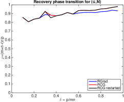
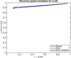
(a)	(b)

Figure 1: Empirical phase transition curves for matrix recovery algorithms: RGrad, RCG, RCG started. Horizontal axis $\delta$ and vertical axis $\rho$ as defined in (20). (a) $\mathcal{G}$ with $m=n=80$, (b) $\mathcal{E}$ with $m=n=800$.

3.2 Computation Time

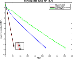
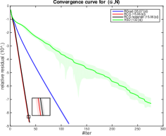
(a)	(b)
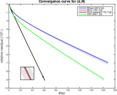
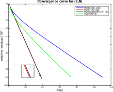
(c)	(d)

Figure 2: Relative residual (mean and standard deviation over ten random tests) as function of number of iterations for Gaussian sensing ((a) and (b)) and entry sensing ((c) and (d)). In Gaussian sensing, $m=n=80$, $r=10$, $1/\rho=2$ (a) or $1/\rho=3$ (b). In entry sensing, $m=n=8000$, $r=100$, $1/\rho=2$ (c) or $1/\rho=3$ (d). The values after each algorithm are the average computational time (seconds) for convergence.

Many algorithms have been designed for the matrix recovery problem, for example [7, 30, 37, 52, 38, 29, 59, 53, 55, 44, 40, 41], just to name a few. Exhaustive comparisons with all those algorithms are impossible. In this section, we will compare RGrad, RCG, RCG restarted with the alternating steepest descend (ASD) method developed in [53]. ASD takes advantage of the product factorization of low rank matrices and minimizes the bi-quadratic function

$$f(L,R)=\frac{1}{2}\left\|y-\mathcal{A}(LR)\right\|_{2}^{2}$$

alternatively with $L$ and $R$, where $L\in\mathbb{R}^{m\times r}$ and $R\in\mathbb{R}^{r\times n}$. In each iteration of ASD, it applies a step of steepest gradient descent on one factor matrix while the other one is held fixed. The efficiency of ASD has been reported in [53] for its low per iteration computational complexity. Indirect comparisons with other algorithms can be made from [53] and references therein.

We compare the algorithms on both Gaussian sensing and entry sensing. For Gaussian sensing, the tests are conducted for $m=n=80$, $r=10$ and $1/\rho\in\{2,3\}$; and for entry sensing, the tests are conducted for $m=n=8000$, $r=100$ and $1/\rho\in\{2,3\}$. The algorithms are terminated when the relative residual is less than $10^{-9}$. The relative residual plotted against the number of iterations is presented in Fig. 2. First it can be observed that the convergence curves for RCG and RCG restarted are almost indistinguishable, differing only in one or two iterations, which again shows the effectiveness of the restarting conditions. A close look at the computational results reveals that restarting usually occurs in the first few iterations for RCG restarted. Moreover, RCG and RCG restarted are sufficiently faster than RGrad and ASD both in terms of the convergence rate and in terms of the average computation time.

4 Proofs of Main Results

4.1 A Key Lemma

The following lemma will be used repeatedly, which contains the second order information of the smooth low rank matrix manifold, see Fig. 3.

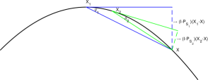
Figure 3: The set of low rank matrices forms a continuous manifold (denoted by a curve here) in the ambient space. From the plot, it is clear that $\left\|\left(I-\mathcal{P}_{\mathcal{S}_{1}}\right)\left(X_{1}-X\right)\right\|_{F}=\left\|X_{1}-X\right\|_{F}\cdot\sin\theta_{1}$ and $\left\|\left(I-\mathcal{P}_{\mathcal{S}_{2}}\right)\left(X_{2}-X\right)\right\|_{F}=\left\|X_{2}-X\right\|_{F}\cdot\sin\theta_{2}$. As $X_{l}$ approaches $X$ ($l=1,2$), the angle also decreases. So $\left\|\left(I-\mathcal{P}_{\mathcal{S}_{l}}\right)\left(X_{l}-X\right)\right\|_{F}=o(\left\|X_{l}-X\right\|_{F})$.

Lemma 4.1.

Let $X_{l}=U_{l}\Sigma_{l}V_{l}$ be a rank $r$ matrix, and $\mathcal{S}_{l}$ be the tangent space of the rank $r$ matrix manifold at $X_{l}$. Let $X$ be another rank $r$ matrix. Then

$$\left\|\left(I-\mathcal{P}_{\mathcal{S}_{l}}\right)X\right\|_{F} \leq\frac{1}{\sigma_{\min}\left(X\right)}\left\|X_{l}-X\right\|_{2}\left\|X_{l}-X\right\|_{F}$$ (21)

$$\leq\frac{1}{\sigma_{\min}\left(X\right)}\left\|X_{l}-X\right\|_{F}^{2}.$$ (22)

The proof of Lem. 4.1 relies on the following result which bounds the projection distance of the singular vector subspaces of two matrices.

Lemma 4.2.

Let $X_{l}=U_{l}\Sigma_{l}V_{l}^{*}$ and $X=U\Sigma V^{*}$ be two rank $r$ matrices. Then

$$\left\|U_{l}U_{l}^{*}-UU^{*}\right\|_{2}\leq\frac{\left\|X_{l}-X\right\|_{2}}{\sigma_{\min}\left(X\right)}\quad\mbox{and}\quad\left\|V_{l}V_{l}^{*}-VV^{*}\right\|_{2}\leq\frac{\left\|X_{l}-X\right\|_{2}}{\sigma_{\min}\left(X\right)};$$ (23)

$$\left\|U_{l}U_{l}^{*}-UU^{*}\right\|_{F}\leq\frac{\sqrt{2}\left\|X_{l}-X\right\|_{F}}{\sigma_{\min}\left(X\right)}\quad\mbox{and}\quad\left\|V_{l}V_{l}^{*}-VV^{*}\right\|_{F}\leq\frac{\sqrt{2}\left\|X_{l}-X\right\|_{F}}{\sigma_{\min}\left(X\right)}.$$ (24)

The proof of Lem. 4.2 is presented in Appendix A.

Proof of Lemma 4.1.

Let $\mathcal{S}$ be the tangent space of the rank $r$ matrix manifold at $X$ as defined in (11). Clearly we have $\mathcal{P}_{\mathcal{S}}\left(X\right)=X$. So

$$\left(I-\mathcal{P}_{\mathcal{S}_{l}}\right)X =\left(\mathcal{P}_{\mathcal{S}}-\mathcal{P}_{\mathcal{S}_{l}}\right)X$$

$$=UU^{*}X+XVV^{*}-UU^{*}XVV^{*}-U_{l}U_{l}^{*}X-XV_{l}V_{l}^{*}+U_{l}U_{l}^{*}XV_{l}V_{l}^{*}$$

$$=\left(UU^{*}-U_{l}U_{l}^{*}\right)X+X\left(VV^{*}-V_{l}V_{l}^{*}\right)$$

$$\quad-UU^{*}XVV^{*}+UU^{*}XV_{l}V_{l}^{*}-UU^{*}XV_{l}V_{l}^{*}+U_{l}U_{l}^{*}XV_{l}V_{l}^{*}$$

$$=\left(UU^{*}-U_{l}U_{l}^{*}\right)X+X\left(VV^{*}-V_{l}V_{l}^{*}\right)$$

$$\quad-\left(UU^{*}-U_{l}U_{l}^{*}\right)XV_{l}V_{l}^{*}-UU^{*}X\left(VV^{*}-V_{l}V_{l}^{*}\right)$$

$$=\left(UU^{*}-U_{l}U_{l}^{*}\right)X\left(I-V_{l}V_{l}^{*}\right)+\left(I-UU^{*}\right)X\left(VV^{*}-V_{l}V_{l}^{*}\right)$$

$$=\left(UU^{*}-U_{l}U_{l}^{*}\right)X\left(I-V_{l}V_{l}^{*}\right)$$

$$=\left(UU^{*}-U_{l}U_{l}^{*}\right)(X-X_{l})\left(I-V_{l}V_{l}^{*}\right),$$ (25)

where the last two equalities follow from the fact $\left(I-UU^{*}\right)X=0$ and $X_{l}(I-V_{l}V_{l}^{*})=0$. Taking the Frobenius norm on both sides of (25) gives

$$\left\|\left(I-\mathcal{P}_{\mathcal{S}_{l}}\right)X\right\|_{F} \leq\left\|UU^{*}-U_{l}U_{l}^{*}\right\|_{2}\left\|X_{l}-X\right\|_{F}\left\|I-V_{l}V_{l}^{*}\right\|_{2}$$

$$\leq\frac{1}{\sigma_{\min}\left(X\right)}\left\|X_{l}-X\right\|_{2}\left\|X_{l}-X\right\|_{F},$$

which completes the proof of (21). Inequality (22) follows directly from the fact $\left\|X_{l}-X\right\|_{2}\leq\left\|X_{l}-X\right\|_{F}$. ∎

4.2 Proof of Theorem 2.1

Though Alg. 3 can be viewed as a restarted variant of Alg. 4 in which restarting occurs in each iteration, we choose to provide a separated proof to Thm. 2.1 in order to highlight the main architecture of the proof. We first list two useful lemmas.

Lemma 4.3.

Let $Z_{1},~{}Z_{2}$ be two low rank matrices. Suppose $\left\langle Z_{1},Z_{2}\right\rangle=0$ and $\mbox{rank}(Z_{1})+\mbox{rank}(Z_{2})\leq\min\left(m,n\right)$. Then

$$\left|\left\langle\mathcal{A}\left(Z_{1}\right),\mathcal{A}\left(Z_{2}\right)\right\rangle\right|\leq R_{\mbox{rank}(Z_{1})+\mbox{rank}(Z_{2})}\left\|Z_{1}\right\|_{F}\left\|Z_{2}\right\|_{F}.$$

This lemma is analogous to Lem. $2.1$ in [14] for compressed sensing. The proof for the low rank matrix version can be found in [17]. We repeat the proof in Appendix B to keep the paper self-contained.

Lemma 4.4.

Let $X_{l}=U_{l}\Sigma_{l}V_{l}^{*}$ be a rank $r$ matrix with the tangent space $\mathcal{S}_{l}$. Let $X$ be another rank $r$ matrix. Then the Frobenius norm of $\mathcal{P}_{\mathcal{S}_{l}}\mathcal{A}^{*}\mathcal{A}\left(I-\mathcal{P}_{\mathcal{S}_{l}}\right)X$ can be bounded as

$$\left\|\mathcal{P}_{\mathcal{S}_{l}}\mathcal{A}^{*}\mathcal{A}\left(I-\mathcal{P}_{\mathcal{S}_{l}}\right)(X)\right\|_{F}\leq R_{3r}\left\|\left(I-\mathcal{P}_{\mathcal{S}_{l}}\right)(X)\right\|_{F}.$$

The proof of Lem. 4.4 is also presented in Appendix B.

Proof of Theorem 2.1.

The proof begins with the following inequality

$$\left\|X_{l+1}-X\right\|_{F}\leq\left\|X_{l+1}-W_{l}\right\|_{F}+\left\|W_{l}-X\right\|_{F}\leq 2\left\|W_{l}-X\right\|_{F},$$

where the last inequality follows from the fact that $X_{l+1}$ is the best rank $r$ approximation of $W_{l}$ in the Frobenius norm. Substituting $W_{l}=X_{l}+\alpha_{l}\mathcal{P}_{\mathcal{S}_{l}}\left(G_{l}\right)$ into the above inequality gives

$$\left\|X_{l+1}-X\right\|_{F} \leq 2\left\|X_{l}+\alpha_{l}\mathcal{P}_{\mathcal{S}_{l}}\left(G_{l}\right)-X\right\|_{F}$$

$$=2\left\|X_{l}+\alpha_{l}\mathcal{P}_{\mathcal{S}_{l}}\mathcal{A}^{*}\left(y-\mathcal{A}\left(X_{l}\right)\right)-X\right\|_{F}$$

$$=2\left\|X_{l}-X-\alpha_{l}\mathcal{P}_{\mathcal{S}_{l}}\mathcal{A}^{*}\mathcal{A}\left(X_{l}-X\right)\right\|_{F}$$

$$\leq 2\left\|X_{l}-X-\alpha_{l}\mathcal{P}_{\mathcal{S}_{l}}\mathcal{A}^{*}\mathcal{A}\mathcal{P}_{\mathcal{S}_{l}}\left(X_{l}-X\right)\right\|_{F}$$

$$\quad+2\alpha_{l}\left\|\mathcal{P}_{\mathcal{S}_{l}}\mathcal{A}^{*}\mathcal{A}\left(I-\mathcal{P}_{\mathcal{S}_{l}}\right)\left(X_{l}-X\right)\right\|_{F}$$

$$\leq 2\left\|\mathcal{P}_{\mathcal{S}_{l}}\left(X_{l}-X\right)-\alpha_{l}\mathcal{P}_{\mathcal{S}_{l}}\mathcal{A}^{*}\mathcal{A}\mathcal{P}_{\mathcal{S}_{l}}\left(X_{l}-X\right)\right\|_{F}$$

$$\quad+2\left\|\left(I-\mathcal{P}_{\mathcal{S}_{l}}\right)\left(X_{l}-X\right)\right\|_{F}$$

$$\quad+2\alpha_{l}\left\|\mathcal{P}_{\mathcal{S}_{l}}\mathcal{A}^{*}\mathcal{A}\left(I-\mathcal{P}_{\mathcal{S}_{l}}\right)\left(X_{l}-X\right)\right\|_{F}$$

$$=2\left\|\left(\mathcal{P}_{\mathcal{S}_{l}}-\alpha_{l}\mathcal{P}_{\mathcal{S}_{l}}\mathcal{A}^{*}\mathcal{A}\mathcal{P}_{\mathcal{S}_{l}}\right)\left(X_{l}-X\right)\right\|_{F}+2\left\|\left(I-\mathcal{P}_{\mathcal{S}_{l}}\right)\left(X\right)\right\|_{F}$$

$$\quad+2\left|\alpha_{l}\right|\left\|\mathcal{P}_{\mathcal{S}_{l}}\mathcal{A}^{*}\mathcal{A}\left(I-\mathcal{P}_{\mathcal{S}_{l}}\right)\left(X\right)\right\|_{F}$$

$$:=I_{1}+I_{2}+I_{3},$$ (26)

where the last inequality follows from the fact $\left(I-\mathcal{P}_{\mathcal{S}_{l}}\right)\left(X_{l}\right)=0$. In the following, we will bound $I_{1}$, $I_{2}$ and $I_{3}$ one by one.

Bound of $I_{1}$. We first consider the spectral norm of $\mathcal{P}_{\mathcal{S}_{l}}-\mathcal{P}_{\mathcal{S}_{l}}\mathcal{A}^{*}\mathcal{A}\mathcal{P}_{\mathcal{S}_{l}}$. Since it is a symmetric operator, we have

$$\left\|\mathcal{P}_{\mathcal{S}_{l}}-\mathcal{P}_{\mathcal{S}_{l}}\mathcal{A}^{*}\mathcal{A}\mathcal{P}_{\mathcal{S}_{l}}\right\| =\sup_{\left\|Z\right\|_{F}=1}\left|\left\langle\left(\mathcal{P}_{\mathcal{S}_{l}}-\mathcal{P}_{\mathcal{S}_{l}}\mathcal{A}^{*}\mathcal{A}\mathcal{P}_{\mathcal{S}_{l}}\right)\left(Z\right),Z\right\rangle\right|$$

$$=\sup_{\left\|Z\right\|_{F}=1}\left|\left\|\mathcal{P}_{\mathcal{S}_{l}}\left(Z\right)\right\|_{F}^{2}-\left\|\mathcal{A}\mathcal{P}_{\mathcal{S}_{l}}\left(Z\right)\right\|_{2}^{2}\right|$$

$$\leq\sup_{\left\|Z\right\|_{F}=1}R_{2r}\left\|\mathcal{P}_{\mathcal{S}_{l}}\left(Z\right)\right\|_{F}^{2}\leq R_{2r},$$ (27)

where the first inequality follows the RIC bound of the sensing operator by noting that $\mbox{rank}\left(\mathcal{P}_{\mathcal{S}_{l}}\left(Z\right)\right)~{}\leq~{}2r$. The RIC based bound for the descent stepsize $\alpha_{l}$ can be obtained as

$$\frac{1}{1+R_{2r}}\leq\alpha_{l}=\frac{\left\|\mathcal{P}_{U_{l}}\left(G_{l}\right)\right\|_{F}^{2}}{\left\|\mathcal{A}\mathcal{P}_{U_{l}}\left(G_{l}\right)\right\|_{2}^{2}}\leq\frac{1}{1-R_{2r}}.$$ (28)

Immediately we have

$$\left|\alpha_{l}-1\right|\leq\frac{R_{2r}}{1-R_{2r}}$$ (29)

Combining (27) and (29) gives the bound of the spectral norm of $\mathcal{P}_{\mathcal{S}_{l}}-\alpha_{l}\mathcal{P}_{\mathcal{S}_{l}}\mathcal{A}^{*}\mathcal{A}\mathcal{P}_{\mathcal{S}_{l}}$

$$\left\|\mathcal{P}_{\mathcal{S}_{l}}-\alpha_{l}\mathcal{P}_{\mathcal{S}_{l}}\mathcal{A}^{*}\mathcal{A}\mathcal{P}_{\mathcal{S}_{l}}\right\| \leq\left\|\mathcal{P}_{\mathcal{S}_{l}}-\mathcal{P}_{\mathcal{S}_{l}}\mathcal{A}^{*}\mathcal{A}\mathcal{P}_{\mathcal{S}_{l}}\right\|+|1-\alpha_{l}|\left\|\mathcal{P}_{\mathcal{S}_{l}}\mathcal{A}^{*}\mathcal{A}\mathcal{P}_{\mathcal{S}_{l}}\right\|$$

$$\leq R_{2r}+\frac{R_{2r}}{1-R_{2r}}\left(1+R_{2r}\right)=\frac{2R_{2r}}{1-R_{2r}}.$$

Thus $I_{1}$ can be bounded as

$$I_{1}\leq\frac{4R_{2r}}{1-R_{2r}}\left\|X_{l}-X\right\|_{F}.$$ (30)

Bound of $I_{2}$. The second term $I_{2}$ can be bounded as

$$I_{2}\leq\frac{2}{\sigma_{\min}\left(X\right)}\left\|X_{l}-X\right\|_{F}^{2}.$$ (31)

by Lem. 4.1.

Bound of $I_{3}$. The third term $I_{3}$ can be bounded by applying Lem 4.4 as follows

$$I_{3} \leq\frac{2R_{3r}}{1-R_{2r}}\left\|\left(I-\mathcal{P}_{\mathcal{S}_{l}}\right)\left(X\right)\right\|_{F}\leq\frac{2R_{3r}}{1-R_{2r}}\left\|X_{l}-X\right\|_{F},$$ (32)

where the second inequality follows from the fact $\left(I-\mathcal{P}_{\mathcal{S}_{l}}\right)\left(X_{l}\right)=0$.

Inserting (30), (31) and (32) into (26) gives

$$\left\|X_{l+1}-X\right\|_{F}\leq\left(\frac{4R_{2r}+2R_{3r}}{1-R_{2r}}+\frac{2}{\sigma_{\min}\left(X\right)}\left\|X_{l}-X\right\|_{F}\right)\left\|X_{l}-X\right\|_{F}.$$ (33)

Initialization. Let $X_{0}=\mathcal{H}_{r}(\mathcal{A}^{*}\left(y\right))$ and $U_{0}\in\mathbb{R}^{m\times r}$ be its left singular vectors. Define $Q_{0}\in\mathbb{R}^{m\times 2r}$ as an orthogonal matrix which spans the column subspaces of $X_{0}$ and $X$. Let $Q_{0}^{\perp}$ be the complement of $Q_{0}$. Since

$$\left\|X_{0}-\mathcal{A}^{*}\left(y\right)\right\|_{F}^{2}=\left\|X_{0}-\mathcal{P}_{Q_{0}}\left(\mathcal{A}^{*}\left(y\right)\right)\right\|_{F}^{2}+\left\|\mathcal{P}_{Q_{0}^{\perp}}\left(\mathcal{A}^{*}\left(y\right)\right)\right\|_{F}^{2}$$

and

$$\left\|X-\mathcal{A}^{*}\left(y\right)\right\|_{F}^{2} =\left\|X-\mathcal{P}_{Q_{0}}\left(\mathcal{A}^{*}\left(y\right)\right)\right\|_{F}^{2}+\left\|\mathcal{P}_{Q_{0}^{\perp}}\left(\mathcal{A}^{*}\left(y\right)\right)\right\|_{F}^{2},$$

the inequality $\left\|X_{0}-\mathcal{A}^{*}\left(y\right)\right\|_{F}\leq\left\|X-\mathcal{A}^{*}\left(y\right)\right\|_{F}$ implies

$$\left\|X_{0}-\mathcal{P}_{Q_{0}}\left(\mathcal{A}^{*}\left(y\right)\right)\right\|_{F}\leq\left\|X-\mathcal{P}_{Q_{0}}\left(\mathcal{A}^{*}\left(y\right)\right)\right\|_{F}.$$ (34)

So we have

$$\left\|X_{0}-X\right\|_{F} \leq\left\|X_{0}-\mathcal{P}_{Q_{0}}\left(\mathcal{A}^{*}\left(y\right)\right)\right\|_{F}+\left\|\mathcal{P}_{Q_{0}}\left(\mathcal{A}^{*}\left(y\right)\right)-X\right\|_{F}$$

$$\leq 2\left\|\mathcal{P}_{Q_{0}}\left(\mathcal{A}^{*}\left(y\right)\right)-X\right\|_{F}$$

$$=2\left\|\left(\mathcal{P}_{Q_{0}}-\mathcal{P}_{Q_{0}}\mathcal{A}^{*}\mathcal{A}\mathcal{P}_{Q_{0}}\right)\left(X\right)\right\|_{F}$$

$$\leq 2R_{2r}\left\|X\right\|_{F},$$ (35)

where the last inequality follows from the RIC based bound of $\mathcal{P}_{Q_{0}}-\mathcal{P}_{Q_{0}}\mathcal{A}^{*}\mathcal{A}\mathcal{P}_{Q_{0}}$ which can be similarly obtained as in (27).

Define

$$\gamma=\frac{4R_{2r}+2R_{3r}}{1-R_{2r}}+\frac{4R_{2r}}{\sigma_{\min}\left(X\right)}\left\|X\right\|_{F}.$$ (36)

If $\gamma<1$, inserting (35) into (33) and proof by induction gives

$$\left\|X_{l+1}-X\right\|_{F}\leq\gamma\left\|X_{l}-X\right\|_{F}.$$ (37)

Moreover, if

$$R_{3r}\leq\frac{\sigma_{\min}\left(X\right)}{\sigma_{\max}\left(X\right)}\cdot\frac{1}{12\sqrt{r}},$$

we have

$$\gamma\leq\frac{6R_{3r}}{1-R_{3r}}+\frac{4R_{3r}\sqrt{r}\sigma_{\max}\left(X\right)}{\sigma_{\min}\left(X\right)}<1,$$ (38)

where we have utilized the fact $R_{2r}\leq R_{3r}$ following from Def. 1.1 and the inequality $\left\|X\right\|_{F}\leq\sqrt{r}\sigma_{\max}\left(X\right)$. ∎

4.3 Proof of Theorem 2.2

The following technical lemma which can be found for example in [7] establishes the convergence of a three term recurrence relation.

Lemma 4.5.

Suppose $c_{0}$, $\tau_{1},~{}\tau_{2}\geq 0$ and let $\mu=\frac{1}{2}\left(\tau_{1}+\sqrt{\tau_{1}^{2}+4\tau_{2}}\right)$. Assume $0\leq c_{1}\leq\mu c_{0}$ and define $0\leq c_{l}\leq\tau_{1,l-1}c_{l-1}+\tau_{2,l-2}c_{l-2}$ with $\tau_{1,l-1}\leq\tau_{1}$ and $\tau_{2,l-2}\leq\tau_{2}$ for $l\geq 2$. If $\tau_{1}+\tau_{2}<1$, then $\mu<1$ and

$$c_{l}\leq\mu^{l}c_{0}.$$ (39)

Lemma 4.6.

When the inequalities in Eq. (16) are satisfied, we have

$$|\beta_{l}|\leq\frac{\kappa_{2}R_{2r}}{1-R_{2r}}+\frac{\kappa_{1}\kappa_{2}}{1-R_{2r}}\quad\mbox{and}\quad|\alpha_{l}-1|\leq\frac{R_{2r}}{(1-R_{2r})-\kappa_{1}(1+R_{2r})}.$$ (40)

Notice that when restarting occurs we have $\beta_{l}=0$ and $\alpha_{l}$ can be bounded as in (29). So the bounds in (40) still apply since $\kappa_{1}\geq 0$ and $\kappa_{2}\geq 0$.

Proof of Lemma 4.6.

We first bound $\beta_{l}$ as follows

$$\left|\beta_{l}\right| =\left|\frac{\left\langle\mathcal{A}\mathcal{P}_{\mathcal{S}_{l}}\left(G_{l}\right),\mathcal{A}\mathcal{P}_{\mathcal{S}_{l}}\left(P_{l-1}\right)\right\rangle}{\left\|\mathcal{A}\mathcal{P}_{\mathcal{S}_{l}}\left(P_{l-1}\right)\right\|_{2}^{2}}\right|$$

$$=\left|\frac{\left\langle\mathcal{P}_{\mathcal{S}_{l}}\left(G_{l}\right),\mathcal{P}_{\mathcal{S}_{l}}\mathcal{A}^{*}\mathcal{A}\mathcal{P}_{\mathcal{S}_{l}}\left(P_{l-1}\right)\right\rangle}{\left\|\mathcal{A}\mathcal{P}_{\mathcal{S}_{l}}\left(P_{l-1}\right)\right\|_{2}^{2}}\right|$$

$$\leq\left|\frac{\left\langle\mathcal{P}_{\mathcal{S}_{l}}\left(G_{l}\right),\left(\mathcal{P}_{\mathcal{S}_{l}}-\mathcal{P}_{\mathcal{S}_{l}}\mathcal{A}^{*}\mathcal{A}\mathcal{P}_{\mathcal{S}_{l}}\right)\left(\mathcal{P}_{\mathcal{S}_{l}}P_{l-1}\right)\right\rangle}{\left\|\mathcal{A}\mathcal{P}_{\mathcal{S}_{l}}\left(P_{l-1}\right)\right\|_{2}^{2}}\right|+\left|\frac{\left\langle\mathcal{P}_{\mathcal{S}_{l}}\left(G_{l}\right),\mathcal{P}_{\mathcal{S}_{l}}\left(P_{l-1}\right)\right\rangle}{\left\|\mathcal{A}\mathcal{P}_{\mathcal{S}_{l}}\left(P_{l-1}\right)\right\|_{2}^{2}}\right|$$

$$\leq\frac{R_{2r}}{1-R_{2r}}\frac{\left\|\mathcal{P}_{\mathcal{S}_{l}}\left(G_{l}\right)\right\|_{F}}{\left\|\mathcal{P}_{\mathcal{S}_{l}}\left(P_{l-1}\right)\right\|_{F}}+\frac{1}{1-R_{2r}}\left|\frac{\left\langle\mathcal{P}_{\mathcal{S}_{l}}\left(G_{l}\right),\mathcal{P}_{\mathcal{S}_{l}}\left(P_{l-1}\right)\right\rangle}{\left\|\mathcal{P}_{\mathcal{S}_{l}}\left(P_{l-1}\right)\right\|_{F}^{2}}\right|$$

$$=\frac{R_{2r}}{1-R_{2r}}\frac{\left\|\mathcal{P}_{\mathcal{S}_{l}}\left(G_{l}\right)\right\|_{F}}{\left\|\mathcal{P}_{\mathcal{S}_{l}}\left(P_{l-1}\right)\right\|_{F}}+\frac{1}{1-R_{2r}}\left|\frac{\left\langle\mathcal{P}_{\mathcal{S}_{l}}\left(G_{l}\right),\mathcal{P}_{\mathcal{S}_{l}}\left(P_{l-1}\right)\right\rangle}{\left\|\mathcal{P}_{\mathcal{S}_{l}}\left(G_{l}\right)\right\|_{F}\left\|\mathcal{P}_{\mathcal{S}_{l}}\left(P_{l-1}\right)\right\|_{F}}\right|\frac{\left\|\mathcal{P}_{\mathcal{S}_{l}}\left(G_{l}\right)\right\|_{F}}{\left\|\mathcal{P}_{\mathcal{S}_{l}}\left(P_{l-1}\right)\right\|_{F}}$$

$$\leq\frac{\kappa_{2}R_{2r}}{1-R_{2r}}+\frac{\kappa_{1}\kappa_{2}}{1-R_{2r}},$$

where the second inequality follows from the RIC bounds of $\mathcal{P}_{\mathcal{S}_{l}}-\mathcal{P}_{\mathcal{S}_{l}}\mathcal{A}^{*}\mathcal{A}\mathcal{P}_{\mathcal{S}_{l}}$ (see (27)) and $\mathcal{A}\mathcal{P}_{\mathcal{S}_{l}}$, and the last inequality follows from (16). To bound $\alpha_{l}$, first note

$$\left|\beta_{l}\left\langle\mathcal{P}_{\mathcal{S}_{l}}\left(G_{l}\right),\mathcal{P}_{\mathcal{S}_{l}}\left(P_{l-1}\right)\right\rangle\right| =\left|\frac{\left\langle\mathcal{A}\mathcal{P}_{\mathcal{S}_{l}}\left(G_{l}\right),\mathcal{A}\mathcal{P}_{\mathcal{S}_{l}}\left(P_{l-1}\right)\right\rangle}{\left\|\mathcal{A}\mathcal{P}_{\mathcal{S}_{l}}\left(P_{l-1}\right)\right\|_{2}^{2}}\left\langle\mathcal{P}_{\mathcal{S}_{l}}\left(G_{l}\right),\mathcal{P}_{\mathcal{S}_{l}}\left(P_{l-1}\right)\right\rangle\right|$$

$$\leq\frac{1+R_{2r}}{1-R_{2r}}\frac{\left\|\mathcal{P}_{\mathcal{S}_{l}}\left(G_{l}\right)\right\|_{F}}{\left\|\mathcal{P}_{\mathcal{S}_{l}}\left(P_{l-1}\right)\right\|_{F}}\left|\left\langle\mathcal{P}_{\mathcal{S}_{l}}\left(G_{l}\right),\mathcal{P}_{\mathcal{S}_{l}}\left(P_{l-1}\right)\right\rangle\right|$$

$$\leq\frac{\kappa_{1}\left(1+R_{2r}\right)}{1-R_{2r}}\left\|\mathcal{P}_{\mathcal{S}_{l}}\left(G_{l}\right)\right\|_{F}^{2},$$

where the last inequality follows from (16). Consequently,

$$\left|\left\langle\mathcal{P}_{\mathcal{S}_{l}}\left(P_{l}\right),\mathcal{P}_{\mathcal{S}_{l}}\left(G_{l}\right)\right\rangle\right| \geq\left\|\mathcal{P}_{\mathcal{S}_{l}}\left(G_{l}\right)\right\|_{F}^{2}-\left|\beta_{l}\left\langle\mathcal{P}_{\mathcal{S}_{l}}\left(G_{l}\right),\mathcal{P}_{\mathcal{S}_{l}}\left(P_{l-1}\right)\right\rangle\right|$$

$$\geq\left(1-\frac{\kappa_{1}\left(1+R_{2r}\right)}{1-R_{2r}}\right)\left\|\mathcal{P}_{\mathcal{S}_{l}}\left(G_{l}\right)\right\|_{F}^{2}$$

and the application of the Cauchy-Schwarz inequality gives

$$\left\|\mathcal{P}_{\mathcal{S}_{l}}\left(G_{l}\right)\right\|_{F}\leq\frac{1}{1-\frac{\kappa_{1}\left(1+R_{2r}\right)}{1-R_{2r}}}\left\|\mathcal{P}_{\mathcal{S}_{l}}\left(P_{l}\right)\right\|_{F}.$$

Since $\alpha_{l}$ can be rewritten as

$$\alpha_{l} =\frac{\left\langle\mathcal{P}_{\mathcal{S}_{l}}\left(G_{l}\right),\mathcal{P}_{\mathcal{S}_{l}}\left(P_{l}\right)\right\rangle}{\left\|\mathcal{A}\mathcal{P}_{\mathcal{S}_{l}}\left(P_{l}\right)\right\|_{2}^{2}}$$

$$=1+\frac{\left\langle\mathcal{P}_{\mathcal{S}_{l}}\left(G_{l}\right),\mathcal{P}_{\mathcal{S}_{l}}\left(P_{l}\right)\right\rangle-\left\langle\mathcal{A}\mathcal{P}_{\mathcal{S}_{l}}\left(G_{l}\right),\mathcal{A}\mathcal{P}_{\mathcal{S}_{l}}\left(P_{l}\right)\right\rangle}{\left\|\mathcal{A}\mathcal{P}_{\mathcal{S}_{l}}\left(P_{l}\right)\right\|_{2}^{2}}$$

$$=1+\frac{\left\langle\mathcal{P}_{\mathcal{S}_{l}}\left(G_{l}\right),\left(\mathcal{P}_{\mathcal{S}_{l}}-\mathcal{P}_{\mathcal{S}_{l}}\mathcal{A}^{*}\mathcal{A}\mathcal{P}_{\mathcal{S}_{l}}\right)\mathcal{P}_{\mathcal{S}_{l}}\left(P_{l}\right)\right\rangle}{\left\|\mathcal{A}\mathcal{P}_{\mathcal{S}_{l}}\left(P_{l}\right)\right\|_{2}^{2}},$$

it follows that

$$\left|\alpha_{l}-1\right|\leq\frac{R_{2r}}{1-R_{2r}}\frac{\left\|\mathcal{P}_{\mathcal{S}_{l}}\left(G_{l}\right)\right\|_{F}}{\left\|\mathcal{P}_{\mathcal{S}_{l}}\left(P_{l}\right)\right\|_{F}}\leq\frac{R_{2r}}{\left(1-R_{2r}\right)-\kappa_{1}\left(1+R_{2r}\right)},$$

which completes the proof. ∎

Proof of Theorem 2.2.

Analogous to (26), we have

$$\left\|X_{l+1}-X\right\|_{F} \leq 2\left\|X_{l}+\alpha_{l}P_{l}-X\right\|_{F}$$

$$=2\left\|X_{l}-X-\alpha\mathcal{P}_{\mathcal{S}_{l}}\mathcal{A}^{*}\mathcal{A}\left(X_{l}-X\right)+\alpha_{l}\beta_{l}\mathcal{P}_{\mathcal{S}_{l}}\left(P_{l-1}\right)\right\|_{F}$$

$$\leq 2\left\|\left(\mathcal{P}_{\mathcal{S}_{l}}-\alpha_{l}\mathcal{P}_{\mathcal{S}_{l}}\mathcal{A}^{*}\mathcal{A}\mathcal{P}_{\mathcal{S}_{l}}\right)\left(X_{l}-X\right)\right\|_{F}+2\left\|\left(I-\mathcal{P}_{\mathcal{S}_{l}}\right)\left(X\right)\right\|_{F}$$

$$\quad+2\left|\alpha_{l}\right|\left\|\mathcal{P}_{\mathcal{S}_{l}}\mathcal{A}^{*}\mathcal{A}\left(I-\mathcal{P}_{\mathcal{S}_{l}}\right)\left(X\right)\right\|_{F}+2\left|\alpha_{l}\right|\left|\beta_{l}\right|\left\|\mathcal{P}_{\mathcal{S}_{l}}\left(P_{l-1}\right)\right\|_{F}$$

$$:=I_{4}+I_{5}+I_{6}+I_{7}.$$

The bound for $I_{5}$ is exactly the same as the bound for $I_{2}$, while $I_{4}$ and $I_{6}$ can be similarly bounded as $I_{1}$ and $I_{3}$, differing only in the bound for $\alpha_{l}$. Combining the bounds for $\alpha_{l}$ (40) and the spetral norm of $\mathcal{P}_{\mathcal{S}_{l}}-\mathcal{P}_{\mathcal{S}_{l}}\mathcal{A}^{*}\mathcal{A}\mathcal{P}_{\mathcal{S}_{l}}$ (27) together gives the bound for the spectral norm of $\mathcal{P}_{\mathcal{S}_{l}}-\alpha_{l}\mathcal{P}_{\mathcal{S}_{l}}\mathcal{A}^{*}\mathcal{A}\mathcal{P}_{\mathcal{S}_{l}}$

$$\left\|\mathcal{P}_{\mathcal{S}_{l}}-\alpha_{l}\mathcal{P}_{\mathcal{S}_{l}}\mathcal{A}^{*}\mathcal{A}\mathcal{P}_{\mathcal{S}_{l}}\right\| \leq\left\|\mathcal{P}_{\mathcal{S}_{l}}-\mathcal{P}_{\mathcal{S}_{l}}\mathcal{A}^{*}\mathcal{A}\mathcal{P}_{\mathcal{S}_{l}}\right\|+\left(1-\alpha_{l}\right)\left\|\mathcal{P}_{\mathcal{S}_{l}}\mathcal{A}^{*}\mathcal{A}\mathcal{P}_{\mathcal{S}_{l}}\right\|$$

$$\leq R_{2r}+\varepsilon_{\alpha}\left(1+R_{2r}\right),$$

where

$$\varepsilon_{\alpha}:=\frac{R_{2r}}{(1-R_{2r})-\kappa_{1}(1+R_{2r})}.$$

So $I_{4}$ can be bounded as

$$I_{4}\leq 2\left(R_{2r}+\varepsilon_{\alpha}\left(1+R_{2r}\right)\right)\left\|X_{l}-X\right\|_{F}.$$ (41)

Inserting the bound for $\alpha_{l}$ into $I_{6}$, together with Lem. 4.4 gives

$$I_{6} \leq 2R_{3r}\left(1+\varepsilon_{\alpha}\right)\left\|\left(I-\mathcal{P}_{\mathcal{S}_{l}}\right)\left(X\right)\right\|_{F}\leq 2R_{3r}\left(1+\varepsilon_{\alpha}\right)\left\|X_{l}-X\right\|_{F}.$$ (42)

To bound $I_{7}$, first note that $\beta_{l}\mathcal{P}_{\mathcal{S}_{l}}P_{l-1}$ can be expressed in terms of all the previous gradients

$$\beta_{l}\mathcal{P}_{\mathcal{S}_{l}}P_{l-1}=\sum_{j=0}^{l-1}\prod_{q=j+1}^{l}\beta_{q}\prod_{k=j}^{l}\mathcal{P}_{\mathcal{S}_{k}}\left(G_{j}\right),\quad l\geq 1.$$ (43)

Inserting (43) into $I_{7}$ gives

$$I_{7} \leq 2\left|\alpha_{l}\right|\sum_{j=0}^{l-1}\prod_{q=j+1}^{l}\left|\beta_{q}\right|\left\|\mathcal{P}_{\mathcal{S}_{j}}\left(G_{j}\right)\right\|_{F}$$

$$\leq 2\left(1+\varepsilon_{\alpha}\right)\sum_{j=0}^{l-1}\varepsilon_{\beta}^{l-j}\left\|\mathcal{P}_{\mathcal{S}_{j}}\mathcal{A}^{*}\mathcal{A}\left(X_{j}-X\right)\right\|_{F}$$

$$\leq 2\left(1+\varepsilon_{\alpha}\right)\left(1+R_{2r}\right)\sum_{j=0}^{l-1}\varepsilon_{\beta}^{l-j}\left\|X_{j}-X\right\|_{F},$$

where in the second inequality

$$\varepsilon_{\beta}:=\frac{\kappa_{2}R_{2r}}{1-R_{2r}}+\frac{\kappa_{1}\kappa_{2}}{1-R_{2r}},$$

and the third inequality follows from

$$\left\|\mathcal{P}_{\mathcal{S}_{j}}\mathcal{A}^{*}\mathcal{A}\left(X_{j}-X\right)\right\|_{F} =\sup_{\left\|Z\right\|_{F}=1}\left\langle\mathcal{P}_{\mathcal{S}_{j}}\mathcal{A}^{*}\mathcal{A}\left(X_{j}-X\right),Z\right\rangle$$

$$=\sup_{\left\|Z\right\|_{F}=1}\left\langle\mathcal{A}\left(X_{j}-X\right),\mathcal{A}\mathcal{P}_{\mathcal{S}_{j}}\left(Z\right)\right\rangle$$

$$\leq\sup_{\left\|Z\right\|_{F}=1}\left\|\mathcal{A}\left(X_{j}-X\right)\right\|_{F}\left\|\mathcal{A}\mathcal{P}_{\mathcal{S}_{j}}\left(Z\right)\right\|$$

$$\leq\sup_{\left\|Z\right\|_{F}=1}\left(1+R_{2r}\right)\left\|X_{j}-X\right\|_{F}\left\|\mathcal{P}_{\mathcal{S}_{j}}\left(Z\right)\right\|_{F}$$

$$\leq\left(1+R_{2r}\right)\left\|X_{j}-X\right\|_{F}.$$

Combining the bounds for $I_{4},~{}I_{5},~{}I_{6}$ and $I_{7}$ together gives

$$\left\|X_{l+1}-X\right\|_{F} \leq\left(2(R_{2r}+R_{3r})(1+\varepsilon_{\alpha})+2\varepsilon_{\alpha}+\frac{2}{\sigma_{\min}\left(X\right)}\left\|X_{l}-X\right\|_{F}\right)\left\|X_{l}-X\right\|_{F}$$

$$\quad+2\left(1+\varepsilon_{\alpha}\right)\left(1+R_{2r}\right)\sum_{j=0}^{l-1}\varepsilon_{\beta}^{l-j}\left\|X_{j}-X\right\|_{F},\quad l\geq 1.$$

When $l=0$, Alg. 4 is exactly the same as Alg. 3, so it follows from (33) that

$$\left\|X_{1}-X\right\|_{F}\leq\left(\frac{4R_{2r}+2R_{3r}}{1-R_{2r}}+\frac{2}{\sigma_{\min}\left(X\right)}\left\|X_{0}-X\right\|_{F}\right)\left\|X_{0}-X\right\|_{F}.$$ (44)

Define $c_{0}=\left\|X_{0}-X\right\|_{F}$,

$$c_{1}=\left(\frac{4R_{2r}+2R_{3r}}{1-R_{2r}}+\frac{2}{\sigma_{\min}\left(X\right)}c_{0}\right)c_{0}$$ (45)

and

$$c_{l+1} =\left(2(R_{2r}+R_{3r})(1+\varepsilon_{\alpha})+2\varepsilon_{\alpha}+\frac{2}{\sigma_{\min}\left(X\right)}c_{l}\right)c_{l}$$

$$\quad+2\left(1+\varepsilon_{\alpha}\right)\left(1+R_{2r}\right)\sum_{j=0}^{l-1}\varepsilon_{\beta}^{l-j}c_{j},\quad l\geq 1,\quad l\geq 1.$$ (46)

Then it is clear that $c_{l}\geq\left\|X_{l}-X\right\|_{F}$ for all $l\geq 0$. Morover, Eq. (46) can be rewritten in a three term recurrence relation

$$c_{l+1} =\left(\varepsilon_{l}+\varepsilon_{\beta}\right)c_{l}+\varepsilon_{\beta}\left(2\left(1+\varepsilon_{\alpha}\right)\left(1+R_{2r}\right)-\varepsilon_{l-1}\right)c_{l-1}$$

$$\leq\left(\varepsilon_{l}+\varepsilon_{\beta}\right)c_{l}+2\varepsilon_{\beta}\left(1+\varepsilon_{\alpha}\right)\left(1+R_{2r}\right)c_{l-1},$$ (47)

where

$$\varepsilon_{0}=\frac{4R_{2r}+2R_{3r}}{1-R_{2r}}+\frac{2}{\sigma_{\min}\left(X\right)}c_{0},$$

$$\varepsilon_{l}=2(R_{2r}+R_{3r})(1+\varepsilon_{\alpha})+2\varepsilon_{\alpha}+\frac{2}{\sigma_{\min}\left(X\right)}c_{l},\quad l\geq 1$$

Define

$${\tau_{1}=2(R_{2r}+R_{3r})(1+\varepsilon_{\alpha})+2\varepsilon_{\alpha}+\frac{4R_{2r}}{\sigma_{\min}\left(X\right)}\left\|X\right\|_{F}+\varepsilon_{\beta}},$$

$$\tau_{2}=2\varepsilon_{\beta}\left(1+\varepsilon_{\alpha}\right)\left(1+R_{2r}\right),$$

$$\mu=\frac{1}{2}\left(\tau_{1}+\sqrt{\tau_{1}^{2}+4\tau_{2}}\right).$$

Inequality (35) implies $c_{0}\leq 2R_{2r}\left\|X\right\|_{F}$. So together with the right inequality of (40), we have $\varepsilon_{0}\leq\tau_{1}<\mu$. Thus if

$$\gamma:=\tau_{1}+\tau_{2}<1,$$ (48)

we have $\mu<1$, and $c_{1}<c_{0}$, which in turn implies

$$\varepsilon_{1}+\varepsilon_{\beta}\leq\left(2(R_{2r}+R_{3r})(1+\varepsilon_{\alpha})+2\varepsilon_{\alpha}+\frac{2}{\sigma_{\min}\left(X\right)}c_{0}\right)+\varepsilon_{\beta}<\tau_{1}.$$

Therefore the application of Lem. 4.5 together with proof by induction implies

$$c_{l}\leq\mu^{l}c_{0}$$

which completes the proof of the first part of Thm. 2.2.

When $\kappa_{1}=0.1$ and $\kappa_{2}=1$, the sufficient condition for $\gamma<1$ can be verified similarly to (38). ∎

5 Discussion and Future Direction

This paper presents theoretical recovery guarantees of a class of Riemannian gradient descent and conjugate gradient algorithms for low rank matrix recovery in terms of the restricted isometry constant of the sensing operator. The main results in Thms. 2.1 and  2.2 depend on the condition number and the rank of the measured matrix. To eliminate the dependence on the condition number, the deflation or stagewise technique in [32] may be similarly applicable for Algs. 3 and 4. However, it should be interesting to develop and analyse preconditioned Riemannian gradient descent and conjugate gradient descent algorithms since they are more favourable in practice. On the other hand, to eliminate the dependence on $\sqrt{r}$, it may be necessary to study the convergence rate of the Riemannian optimization algorithms in terms of the matrix operator norm rather than the Frobenius norm. However, the contraction of iterates under the matrix operator norm remains a question. In this paper, we have discussed a restarted variant of the Riemannian conjugate gradient descent algorithm with the selection of $\beta_{l}$ being developed in [7], and guarantee analysis for the other selections of $\beta_{l}$ in (8) as well as for different Riemannian metric [43, 40] is also an interesting research topic.

The Riemannian gradient descent and conjugate gradient descent algorithms presented in this paper apply equally to other low rank recovery problems with difference measurement models, such as phase retrieval [25, 16, 15, 57] and blind deconvolution [2] where the underlying matrix after lifting is rank one. This line of research will be pursued independently in the future. Since the condition number of a rank one matrix is always equal to one, it is worth investigating whether we can obtain similar recovery guarantees for phase retrieval and blind deconvolution, but directly in terms of the sampling complexity and without explicit dependence on the condition number of the underlying matrix. Finally, it may be possible to generalize the notion in low rank matrix manifold, for example the restricted isometry constant, to the abstract framework of Riemannian manifold and then extend the analysis in this paper to more general Riemannian gradient descent and conjugate gradient descent algorithms.

Appendix A Proof of Lemma 4.2

We only prove the left inequalities in (23) and (24) and the right inequalities can be similarly established. The left inequality of (23) follows from direct calculations

$$\left\|U_{l}U_{l}^{*}-UU^{*}\right\|_{2} =\left\|UU^{*}\left(I-U_{l}U_{l}^{*}\right)\right\|_{2}=\left\|\left(I-U_{l}U_{l}^{*}\right)UU^{*}\right\|_{2}$$

$$=\left\|\left(I-U_{l}U_{l}^{*}\right)XV\Sigma^{-1}U^{*}\right\|_{2}$$

$$=\left\|\left(I-U_{l}U_{l}^{*}\right)\left(X_{l}-X\right)V\Sigma^{-1}U^{*}\right\|_{2}$$

$$\leq\left\|I-U_{l}U_{l}^{*}\right\|_{2}\left\|X_{l}-X\right\|_{2}\left\|V\right\|_{2}\left\|\Sigma^{-1}\right\|_{2}\left\|U^{*}\right\|_{2}$$

$$=\frac{\left\|X_{l}-X\right\|_{2}}{\sigma_{\min}\left(X\right)},$$

where the first equality follows from a standard result in textbook, see for example [27, Thm. 2.6.1], and the fourth equality follows from the fact $\left(I-U_{l}U_{l}^{*}\right)X_{l}=0$.

To prove the left inequality of (24), we first show that

$$\left\|\left(I-U_{l}U_{l}^{*}\right)UU^{*}\right\|_{F}=\left\|U_{l}U_{l}^{*}\left(I-UU^{*}\right)\right\|_{F}.$$ (49)

Equality (49) can be obtained by noting that

$$\left\|\left(I-U_{l}U_{l}^{*}\right)UU^{*}\right\|_{F}^{2} =\left\langle\left(I-U_{l}U_{l}^{*}\right)UU^{*},\left(I-U_{l}U_{l}^{*}\right)UU^{*}\right\rangle$$

$$=\left\langle I-U_{l}U_{l}^{*},UU^{*}\right\rangle=r-\left\langle U_{l}U_{l}^{*},UU^{*}\right\rangle$$

and

$$\left\|U_{l}U_{l}^{*}\left(I-UU^{*}\right)\right\|_{F}^{2} =\left\langle U_{l}U_{l}^{*}\left(I-UU^{*}\right),U_{l}U_{l}^{*}\left(I-UU^{*}\right)\right\rangle$$

$$=\left\langle U_{l}U_{l}^{*},I-UU^{*}\right\rangle=r-\left\langle U_{l}U_{l}^{*},UU^{*}\right\rangle.$$

So it follows that

$$\left\|U_{l}U_{l}^{*}-UU^{*}\right\|_{F} =\sqrt{2}\left\|\left(I-U_{l}U_{l}^{*}\right)UU^{*}\right\|_{F}$$

$$=\sqrt{2}\left\|\left(I-U_{l}U_{l}^{*}\right)XV\Sigma^{-1}U^{*}\right\|_{F}$$

$$=\sqrt{2}\left\|\left(I-U_{l}U_{l}^{*}\right)\left(X_{l}-X\right)V\Sigma^{-1}U^{*}\right\|_{F}$$

$$\leq\sqrt{2}\left\|I-U_{l}U_{l}^{*}\right\|_{2}\left\|X_{l}-X\right\|_{F}\left\|V\right\|_{2}\left\|\Sigma^{-1}\right\|_{2}\left\|U^{*}\right\|_{2}$$

$$=\frac{\sqrt{2}\left\|X_{l}-X\right\|_{F}}{\sigma_{\min}\left(X\right)}.$$

Appendix B Proofs of Lemmas 4.3 and 4.4

Proof of Lemma 4.3.

The proof follows that for [14, Lem. 2.1] in compressed sensing. Without loss of generality, assume $\left\|Z_{1}\right\|_{F}=1$ and $\left\|Z_{2}\right\|_{F}=1$. Then the application of the RIC bounds gives

$$\left(1-R_{rank(Z_{1})+rank(Z_{2})}\right)\left\|Z_{1}\pm Z_{2}\right\|_{F}^{2}\leq\left\|\mathcal{A}\left(Z_{1}\pm Z_{2}\right)\right\|_{2}^{2},$$

$$\left(1+R_{rank(Z_{1})+rank(Z_{2})}\right)\left\|Z_{1}\pm Z_{2}\right\|_{F}^{2}\geq\left\|\mathcal{A}\left(Z_{1}\pm Z_{2}\right)\right\|_{2}^{2}.$$

Since $\left\langle Z_{1},Z_{2}\right\rangle=0$, we have $\left\|Z_{1}\pm Z_{2}\right\|_{F}^{2}=2$. So

$$2\left(1-R_{rank(Z_{1})+rank(Z_{2})}\right)\leq\left\|\mathcal{A}\left(Z_{1}\pm Z_{2}\right)\right\|_{2}^{2}\leq 2\left(1+R_{rank(Z_{1})+rank(Z_{2})}\right).$$

Finally the parallelogram identity gives

$$\left|\left\langle\mathcal{A}\left(Z_{1}\right),\mathcal{A}\left(Z_{2}\right)\right\rangle\right|=\frac{1}{4}\left|\left\|\mathcal{A}\left(Z_{1}+Z_{2}\right)\right\|_{2}^{2}-\left\|\mathcal{A}\left(Z_{1}-Z_{2}\right)\right\|_{2}^{2}\right|\leq R_{rank(Z_{1})+rank(Z_{2})},$$

which completes the proof. ∎

Proof of Lemma 4.4.

$$\left\|\mathcal{P}_{\mathcal{S}_{l}}\mathcal{A}^{*}\mathcal{A}\left(I-\mathcal{P}_{\mathcal{S}_{l}}\right)(X)\right\|_{F} =\sup_{\left\|Z\right\|_{F}=1}\left|\left\langle\mathcal{P}_{\mathcal{S}_{l}}\mathcal{A}^{*}\mathcal{A}\left(I-\mathcal{P}_{\mathcal{S}_{l}}\right)(X),Z\right\rangle\right|$$

$$=\sup_{\left\|Z\right\|_{F}=1}\left|\left\langle\mathcal{A}\left(I-\mathcal{P}_{\mathcal{S}_{l}}\right)(X),\mathcal{A}\mathcal{P}_{\mathcal{S}_{l}}(Z)\right\rangle\right|$$

$$\leq\sup_{\left\|Z\right\|_{F}=1}R_{3r}\left\|\left(I-\mathcal{P}_{\mathcal{S}_{l}}\right)(X)\right\|_{F}\left\|\mathcal{P}_{\mathcal{S}_{l}}(Z)\right\|_{F}$$

$$\leq R_{3r}\left\|\left(I-\mathcal{P}_{\mathcal{S}_{l}}\right)(X)\right\|_{F},$$

where the second to last inequality follows from Lem. 4.3 together with the fact $\mbox{rank}\left(\left(I-\mathcal{P}_{\mathcal{S}_{l}}\right)(X)\right)\leq r$ and $\mbox{rank}\left(\mathcal{P}_{\mathcal{S}_{l}}(Z)\right)\leq 2r$. ∎

References

• [1] P.-A. Absil, R. Mahony, and R. Sepulchre. Optimization Algorithms on Matrix Manifolds. Princeton University Press, 2008.
• [2] A. Ahmed, B. Recht, and J. Romberg. Blind deconvolution using convex programming. IEEE Transactions on Information Theory, 60(3):1711–1732, 2013.
• [3] D. Amelunxen, M. Lotz, M. B. McCoy, and J. A. Tropp. Living on the edge: A geometric theory of phase transitions in convex optimization. Information and Inference, 3(3):224–294, 2014.
• [4] Y. Amit, M. Fink, N. Srebro, and S. Ullman. Uncovering shared structures in multiclass classification. In Proceedings of the 24th International Conference on Machine Learning, 2007.
• [5] A. Argyriou, T. Evgeniou, and M. Pontil. Multi-task feature learning. In Advances in Neural Information Processing Systems, 2007.
• [6] S. Bhojanapalli, A. Kyrillidis, and S. Sanghavi. Dropping convexity for faster semi-definite optimization. arXiv::1509.03917, 2015.
• [7] J. Blanchard, J. Tanner, and K. Wei. CGIHT: Conjugate gradient iterative hard thresholding for compressed sensing and matrix completion. Information and Inference, 4(4):289–327, 2015.
• [8] J. D. Blanchard, J. Tanner, and K. Wei. Conjugate gradient iterative hard thresholding: Observed noise stability for compressed sensing. IEEE Transactions on Signal Processing, 63(2):528–537, 2015.
• [9] T. Blumensath and M. E. Davies. Iterative hard thresholding for compressed sensing. Applied and Computational Harmonic Analysis, 27(3):265–274, 2009.
• [10] T. Blumensath and M. E. Davies. Normalized iterative hard thresholding: Guaranteed stability and performance. IEEE Journal of Selected Topics in Signal Processing, 4(2):298–309, 2010.
• [11] J.-F. Cai, E. J. Candès, and Z. Shen. A singular value thresholding algorithm for matrix completion. SIAM Journal on Optimization, 20(4):1956–1982, 2010.
• [12] L. Cambier and P.-A. Absil. Robust low-rank matrix completion by riemannian optimization. SIAM Journal on Scientific Computing, 2016. To appear.
• [13] E. J. Candès. Compressive sampling. In International Congress of Mathematics, 2006.
• [14] E. J. Candès. The restricted isometry property and its implications for compressed sensing. Comptes Rendus de l’Acandemie Des Sciences, Serie I:589–592, 2008.
• [15] E. J. Candès, Y. Eldar, T. Strohmer, and V. Voroninski. Phase retrieval via matrix completion. SIAM J. on Imaging Sciences, 6(1):199–225, 2013.
• [16] E. J. Candès, X. Li, and M. Soltanolkotabi. Phase retrieval via Wirtinger flow: Theory and algorithms. IEEE Transactions on Information Theory, 61(4):1985–2007, 2015.
• [17] E. J. Candès and Y. Plan. Tight oracle bounds for low-rank matrix recovery from a minimal number of random measurements. IEEE Transactions on Information Theory, 57(4):2342–2359, 2009.
• [18] E. J. Candès and B. Recht. Exact matrix completion via convex optimization. Foundations of Computational Mathematics, 9(6):717–772, 2009.
• [19] E. J. Candès, J. Romberg, and T. Tao. Robust uncertainty principles: Exact signal reconstruction from highly incomplete frequency information. IEEE Transactions on Information Theory, 52(2):489–509, 2006.
• [20] E. J. Candès and T. Tao. Decoding by linear programming. IEEE Transactions on Information Theory, 51(12):4203–4215, 2005.
• [21] E. J. Candès and T. Tao. The power of convex relaxation: Near-optimal matrix completion. IEEE Transactions on Information Theory, 56(5):2053–1080, 2009.
• [22] Y. Chen and M. J. Wainwright. Fast low-rank estimation by projected gradient descent: General statistical and algorithmic guarantees. arXiv:1509.03025, 2015.
• [23] D. L. Donoho. Compressed sensing. IEEE Transactions on Information Theory, 52(4):1289–1306, 2006.
• [24] L. Eldén. Matrix Methods in Data Mining and Pattern Recogonization. SIAM, 2007.
• [25] R. W. Gerchberg and W. O. Saxton. A practical algorithm for the determination of the phase from image and diffraction plane pictures. Optik, 35(237):237–246, 1972.
• [26] D. Goldfarb and S. Ma. Convergence of fixed-point continuation algorithms for matrix rank minimization. Foundations of Computational Mathematics, 11(2):183–210, 2011.
• [27] G. H. Golub and C. F. Van Loan. Matrix Computations. Johns Hopkins Press, 2013.
• [28] D. Gross. Recovering low-rank matrices from few coefficients in any basis. IEEE Transactions on Information Theory, 57(3):1548–1566, 2011.
• [29] J. P. Haldar and D. Hernando. Rank-constrained solutions to linear matrix equations using PowerFactorization. IEEE Signal Processing Letters, 16(7):584–587, 2009.
• [30] P. Jain, R. Meka, and I. Dhillon. Guaranteed rank minimization via singular value projection. In Proceedings of the Neural Information Processing Systems Conference, 2010.
• [31] P. Jain and P. Netrapalli. Fast exact matrix completion with finite samples. JMLR: Workshop and Conference Proceedings, 40:1–28, 2015.
• [32] P. Jain, P. Netrapalli, and S. Sanghavi. Low-rank matrix completion using alternating minimization. arXiv:1212.0467, 2012.
• [33] M. Kabanava, R. Kueng, H. Rauhut, and Ulrich Terstiege. Stable low-rank matrix recovery via null space properties. arXiv:1507.07184, 2015.
• [34] R. H. Keshavan. Efficient algorithms for collaborative filtering. Ph. D. dissertation, Stanford University, 2012.
• [35] R. H. Keshavan, A. Montanari, and S. Oh. Matrix completion from a few entries. IEEE Transactions on Information Theory, 56(6):2980–2998, 2010.
• [36] R. H. Keshavan, A. Montanari, and S. Oh. Matrix completion from noisy entries. Journal of Machine Learning Research, 11:2057–2078, 2010.
• [37] A. Kyrillidis and V. Cevher. Matrix recipes for hard thresholding methods. Journal of Mathematical Imaging and Vision, 48(2):235–265, 2014.
• [38] K. Lee and Y. Bresler. ADMiRA: Atomic decomposition for minimum rank approximation. IEEE Transactions on Information Theory, 128(1):4402–4416, 2010.
• [39] Z. Liu and L. Vandenberghe. Interior-point method for nuclear norm approximation with application to system identification. SIAM Journal on Matrix Analysis and Applications, 31(3):1235–1256, 2009.
• [40] B. Mishra, K. Adithya Apuroop, and R. Sepulchre. A Riemannian geometry for low-rank matrix completion. arXiv:1211.1550, 2012.
• [41] B. Mishra, G. Meyer, S. Bonnabel, and R. Sepulchre. Fixed-rank matrix factorizations and Riemannian low-rank optimization. Computational Statistics, 29(3):591–261, 2014.
• [42] B. Mishra and R. Sepulchre. R3MC: A Riemannian three-factor algorithm for low-rank matrix completion. arXiv:1306.2672, 2013.
• [43] B. Mishra and R. Sepulchre. Riemannian preconditioning. SIAM Journal on optimization, 26(1):635–660, 2016.
• [44] T. Ngo and Y. Saad. Scaled gradients on Grassmann manifolds for matrix completion. In Advances in Neural Information Processing Systems, 2012.
• [45] J. Nocedal and S. J. Wright. Numerical Optimization. Springer, 2006.
• [46] S. Oymak and B. Hassibi. New null space results and recovery thresholds for matrix rank minimization. arXiv:1011.6326, 2010.
• [47] B. Recht. A simpler approach to matrix completion. The Journal of Machine Learning Research, 12:3413–3430, 2011.
• [48] B. Recht, M. Fazel, and P. A. Parrilo. Guaranteed minimum-rank solutions of linear matrix equations via nuclear norm minimization. SIAM Review, 52(3):471–501, 2010.
• [49] B. Recht, W. Xu, and B. Hassibi. Null space conditions and thresholds for rank minimization. Mathematical Programming Series B, 127:175–211, 2011.
• [50] C. De Sa, K. Olukotun, and C. Ré. Global convergence of stochastic gradient descent for some nonconvex matrix problems. In ICML, 2015.
• [51] R. Sun and Z. Luo. Guaranteed matrix completion via non-convex factorization. In FOCS, 2015.
• [52] J. Tanner and K. Wei. Normalized iterative hard thresholding for matrix completion. SIAM Journal on Scientific Computing, 35(5):S104–S125, 2013.
• [53] J. Tanner and K. Wei. Low rank matrix completion by alternating steepest descent methods. Applied and Computational Harmonic Analysis, 40(2):417–429, 2016.
• [54] S. Tu, R. Boczar, M. Simchowitz, M. Soltanolkotabi, and B. Recht. Low-rank solutions of linear matrix equations via Procrustes flow. arXiv:1507.03566, 2016.
• [55] B. Vandereycken. Low rank matrix completion by Riemannian optimization. SIAM Journal on Optimization, 23(2):1214–1236, 2013.
• [56] K. Wei. Efficient algorithms for compressed sensing and matrix completion. Doctoral thesis, University of Oxford, 2014.
• [57] K. Wei. Solving systems of phaseless equations via Kaczmarz methods: A proof of concept study. Inverse Problems, 31(12):125008, 2015.
• [58] K. Wei, J.-F. Cai, T. F. Chan, and S. Leung. Guarantees of Riemannian optimization for low rank matrix completion. arXiv:1603.06610, 2016.
• [59] Z. Wen, W. Yin, and Y. Zhang. Solving a low-rank factorization model for matrix completion by a non-linear successive over-relaxation algorithm. Mathematical Programming Computation, 4(4):333–361, 2012.
• [60] C. D. White, S. Sanghavi, and R. Ward. The local convexity of solving systems of quadratic equations. arXiv::1506.07868, 2015.
• [61] T. Zhao, Z. Wang, and H. Liu. Nonconvex low rank matrix factorization via inexact first order oracle. In NIPS, 2015.
• [62] Q. Zheng and J. Lafferty. A convergent gradient descent algorithm for rank minimization and semidefinite programming from random linear measurements. In NIPS, 2015.