Living in a Superposition

Abstract

This essay considers a model quantum universe consisting of a very large box containing a screen with two slits and an observer (us) that can pass though the slits. We apply the modern quantum mechanics of closed systems to calculate the probabilities for alternative histories of how we move through the universe and what we see. After passing through the screen with the slits, the quantum state of the universe is a superposition of classically distinguishable histories. We are then living in a superposition. Some frequently asked questions about such situations are answered using this model. The model’s relationship to more realistic quantum cosmologies is briefly discussed.

I Introduction

The two-slit thought experiment sketched in Figure 1 is the simplest and clearest way of illustrating the phenomena of quantum coherence and decoherence. The characteristic pattern of places of arrival at the far screen is evidence of quantum interference. Feynman in his basic physics lectures says the two-slit experiment is “at the heart of quantum mechanics …. [containing its] only mystery” Feylect .

This pedagogical essay uses a variation of the two-slit thought experiment to introduce, illustrate and clarify various aspects of the modern formulation of the quantum mechanics of closed systems, most generally the universe as a whole. This formulation is called decoherent (or consistent) histories quantum mechanics (DH) and is the work of many. In applying quantum mechanics to closed systems like the universe DH can be viewed as an extension, clarification, and to some extend a completion of the work begun by Everett Eve57 .

Essential features of DH can already be understood in the context of the two-slit experiment. The most general objective a quantum theory of a closed system is the prediction of probabilities for alternative histories of how it evolves in time — probabilities for the history of what happened in the early universe for example. But quantum interference is an obstacle to assigning probabilities to sets of alternative histories. In the two-slit experiment it is not possible to assign probabilities to the alternative histories in which the electron arrives at $y$ having gone through the upper or lower slit. The probability to arrive at $y$ should be the sum of the probabilities of the two histories. But in quantum mechanics probabilities are squares of amplitudes and $|\psi_{L}(y)+\psi_{U}(y)|^{2}\not=|\psi_{L}(y)|^{2}+|\psi_{U}(y)|^{2}$ because of interference. A different physical situation illustrated in Figure 2 where the electron interacts with apparatus that measures which slit it passed through. Quantum interference is destroyed and the set of two histories is said to decohere. Consistent probabilities can then be assigned to these histories. In a closed system probabilities can be consistently assigned only to sets of histories that decohere as a consequence of the system’s state and Hamiltonian.

Figure 1: The two-slit experiment. An electron gun at left emits an electron which is detected at a point $y$ on a screen after passing through another screen with two slits. The interference pattern in arrival positions that appears on the screen is a consequence of quantum interference between a history where the electron went through the upper slit and a history where it went through the lower slit.

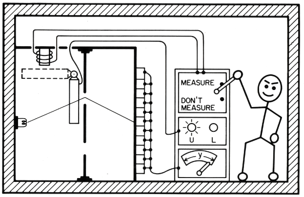
Figure 2: A different model closed system. This picture is meant to suggest a closed system that models a laboratory measurement of a two-slit situation like those referred to in Figure 1. A box contains both a two-slit set-up and an observer reading the results. The observer is outside the two-slit subsystem being measured but inside the box. Measuring whether the electron went through the upper slit destroys the quantum coherence between between histories specifying which slit so that probabilities can be assigned to the outcomes of the measurement. Such models can also be discussed quantum mechanically but in this paper we are discussing observers that are not outside a two-slit system, but rather inside one.

The quantum interference modeled by the two-slit experiment has been seen in many beautiful and important experiments e.g. Ton89 ; AHHZ05 ; hotbucky ; JMMetal12 ; Friedetal00 using increasingly larger interfering systems over time — molecules more than a thousand au for example JMMetal12 . Some distinguished scientists expect quantum coherence to break down for sufficiently large systems (e.g. LG85 ; Pen96 ) but so far there is no evidence for that, and no evidence that quantum interference phenomena could not be seen for much larger systems.

Could we, as human observers, be sent through a very large two-slit experiment as in Figure 3? What would we observe as we travel through the screen with the slits and where would we predict we arrive at the farther screen? This paper addresses such questions in the context of DH utilizing a simple model closed system. We are not discussing the feasibility of carrying out such an experiment. We aim rather at a simple thought experiment to illustrate concretely elements of the quantum mechanics of closed systems.

Beyond calculating predictions for our observations we use this example and DH to answer a number of frequently asked questions: Are we living in a superposition? If so why don’t we see a superposition? Are we smeared out in space? Is the quantum state reduced when we make an observation? etc.

As Feynman emphasized, the essential features of the textbook quantum mechanics of measurement outcomes can be illustrated by the two-slit experiment. Here, we shall find that the essential features of the modern quantum mechanics of closed systems (DH) can be illustrated with the two slit model universe.

The essay is structured as follows: Section II describes the model two-slit universe with an observer carrying a detector. The decoherent histories quantum mechanics of this system is described in Section III and used to calculate the predictions for the our observations in Section IV. The frequently asked questions mentioned above are discussed and answered in Section V. Section VI concludes with a discussion of the relation of this example to realistic quantum cosmology.

II A Model Two-Slit Universe

Imagine a large box containing a very large two-slit apparatus as illustrated in Figure 3 together with a single observer (us) equipped with apparatus for survival and observation as described more fully below. We stress that everything relevant for our discussion is inside the box and that nothing outside is interacting with it. We are not considering a system with an observer outside making measurements on a subsystem as in Figure 2. The box is the universe. We abbreviate ‘two-slit model universe’ by TSMU.

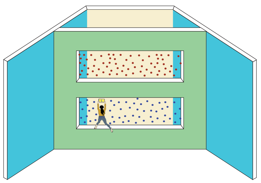
Figure 3: A closed system (TSMU) consisting of a very large two-slit apparatus in a closed box together with an observer (us) carrying a radiation detector that goes through a slit and reaches some point on the farther screen. The top and front of the box have been omitted in the figure to aid visualization but no photons or other information are getting in or out through them. There is a gas of radiation (red) with wavelength $\lambda_{U}$ near the upper slit, and a gas of radiation (blue) with wavelength $\lambda_{L}$ near the lower slit. The observer’s detector records the presence of radiation and its wavelength. As pictured, the observer is going through the lower slit recording the blue radiation there with her detector.

We now specify the contents of the box in a little more detail. In the neighborhood of each slit there is a gas of radiation. Near the upper slit the radiation has wavelength $\lambda_{U}\ll d$ where $d$ is the distance between the slits. The radiation near the lower slit has a different wavelength $\lambda_{L}\ll d$. By measuring the wavelengths on the journey through the slits an observer can tell which slit he or she is passing through.

To make these measurements we suppose that the observer is equipped with detector that can measure which of three states the radiation is in. The three states $\chi_{m}$ are labeled $m=0,1,2$ having energy levels $0,\hbar/\lambda_{U},\hbar/\lambda_{L}$ respectively. The detector starts its journey in the ground state $0$. Levels $1$ and $2$ will be excited if it passes through the upper or lower slit respectively. We assume that the observer’s center of mass degree of freedom is negligibly affected by either kind of radiation.

The excitation of the detector creates a record of which slit the observer passed through. If the excitation is to the level $1$ with energy $\hbar/\lambda_{U}$ then the observer passed through the upper slit, and if to level $2$ with energy $\hbar/\lambda_{L}$ then it was the lower slit. If the decay time of these levels is long compared to the travel time to the farther screen then the observer can be said to have a memory of which slit was passed through. That record constitutes a piece of data on which the observer can condition to construct probabilities for further observations as we see in Section IV.

Eventually the observer and detector reach the screen at the far end of the box. To describe their vertical position there we divide the height up into discrete intervals of length $\Delta$. These are labeled by a discrete variable $Y$, $Y=1,2,\cdots$.

We next discuss the quantum mechanics of this model.

III The Quantum Mechanics of the Model

III.1 The Wave Function of the Universe

The only degrees of freedom that we follow in this model universe are the center of mass position of the observer and the state of the radiation detector. The box, slits, screen, radiation, etc are all considered classically. It would be more realistic to consider them quantum mechanically, but we aim at a simple model. For further simplification we assume symmetry in the direction along the slits. The model is thus effectively two-dimensional as illustrated in Figure 4. The configuration space of the model universe is therefore spanned by the $(x,y)$ coordinates of the observer’s center of mass and the three states of the detector $m=0,1,2$.

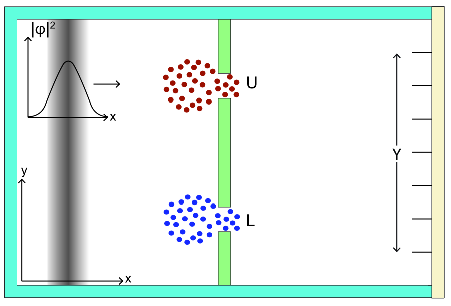
Figure 4: A two dimensional slice through the box in Figure 3. This is useful because we assume symmetry in the transverse direction. The slice is shown at time $t_{0}$ when the wave function of the observer’s center of mass is a narrow wave packet $\phi(x,t)$ in the $x$-direction (inset) (cf (3.2)). The packet is moving toward the right so as to arrive at the slits at time $t_{S}$ and at the farther screen at time $t_{D}$. There is a gas of radiation of wavelength $\lambda_{U}$ near the upper slit (red) and a cloud with a different wavelength $\lambda_{L}$ near the lower slit (blue). We consider a set of alternative histories defined by alternatives at just two times: Whether the observer went though the upper ($U)$ or lower ($L$) slit at time $t_{S}$, and what interval $Y$ the observer arrived at the the farther screen at time $t_{D}$.

The inputs to prediction are the Hamiltonian $H$ and the quantum state of the model universe $|\Psi(t)\rangle$. This is a function of time $t$ in the Schrödinger picture in which we work throughout. The state can be described by a wave function on configuration space, viz.

$$\Psi=\Psi(x,y,m,t).$$ (3.1)

We move back and forth between wave functions like (3.1) and the representation in terms of bras and kets like $|\Psi(t)\rangle$ as convenient.

It is important to note that the observer’s degrees of freedom and the registrations of the apparatus are inside the closed system not outside it. Their degrees of freedom are arguments of the wave function just like any others.

At the starting time $t_{0}$ we take the wave function of the model universe to be

$$\Psi(x,y,m,t_{0})=\phi(x,t_{0})\delta_{0m},\quad t_{0}<t<t_{S}.$$ (3.2)

where $\phi(x,t_{0})$ is a narrow wave packet peaked to the left of the slits but moving to the right so as to reach the slits at time $t_{S}$ and the detecting screen at $t_{D}$ as shown in Figure 4. For simplicity we assume that there is no $y$ dependence of the initial wave function over the height of the box. Thus, progress in $x$ recapitulates evolution in time. The wave function evolves in time by the Schrödinger equation

$$i\hbar\frac{\partial\Psi}{\partial t}=H\Psi$$ (3.3)

where the Hamiltonian $H$ describes the evolution of the observer’s center of mass position in the presence of the impenetrable walls and the interaction of the detector with the radiation. We won’t solve this equation explicitly but rather posit the plausible forms of the solutions.

After passing through the slits the wave function of observer and detector has the form

$$\Psi(x,y,m,t)=\psi_{U}(y,t)\phi(x,t)\delta_{m1}+\psi_{L}(y,t)\phi(x,t)\delta_{m2},\quad t_{S}<t<t_{D}.$$ (3.4)

Here, in the first term $\psi_{U}(y,t)$ is localized near the upper slit at time $t_{S}$ and spreads over a larger region of $y$ by the time $t_{D}$ that the observer hits the detecting screen. The detector is excited to the level $1$ at time $t_{S}$ and remains in that state of excitation for the rest of the journey to the screen at time $t_{D}$. Similarly for the second term.

III.2 Histories

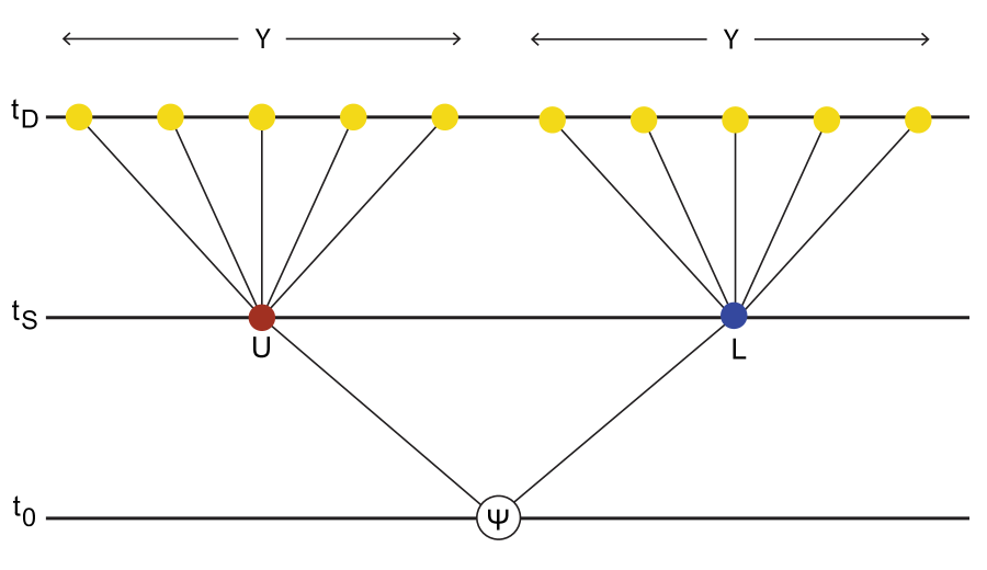
Figure 5: A traditional representation of the set of alternative histories discussed in this section. Time runs upward. Each path from $t_{0}$ to $t_{D}$ corresponds to a history in which the observer and detector went through one slit $S$ ($U$ or $L$) at time $t_{S}$ and arrived at one interval $Y$ at time $t_{D}$. The branching structure of the set is evident. The initial wave function $\Psi$ divides into further branch wave functions at each step. When all the branch wave functions are mutually orthogonal the set of histories decoheres.

Suppose that the observer and detector arrive at position interval $Y$ the screen. What are the probabilities that they went through the upper slit ($U$) or lower slit ($L$) on the way there? These are each the probability of a history — a sequence of events at a series of times. In this case there are just two times — the time $t_{S}$ that the observer and detector reach the slits, and and the time $t_{D}$ that it they reach the screen. The individual histories in an exhaustive set of alternative histories are labeled by $(Y,S)$ where $S$ is $U$ or $L$.

A set of histories like $\{Y,S\}$ has a branching structure illustrated in Figure 5. A wave function called a ‘branch wave function’ can be associated with each history. The initial wave function divides into two branch wave functions at time $t_{S}$ and each of those divides into branches for different $Y$’s at time $t_{D}$. The initial wave function is a sum of all the branch wave functions. As we will discuss in the next section, when it is consistent to assign probabilities to a set of histories their probabilities are norms of corresponding branch wave functions.

There is a general procedure for constructing branch wave functions from projection operators at representing alternatives at different times. But the set $\{Y,S\}$ is so simple we can read the results off of (3.4). The branch wave functions $\Psi_{YS}(x,y,m,t)$ are the two parts of (3.4) restricted to the various values of $Y$.

The restriction to the intervals $Y$ can be made more explicit by introducing projection operators $P_{Y}$ that are 1 for $y$’s inside the interval $Y$ and zero for $y$’s outside it. These satisfy

$$P_{Y}P_{Y^{\prime}}=\delta_{YY^{\prime}},\quad\sum_{Y}P_{Y}=I$$ (3.5)

showing that they are an exclusive and exhaustive set of projections.

The branch wave functions for the set $\{Y,S\}$ at the last time in the histories $t_{D}$ are then, from (3.4),

$$\Psi_{YU}(x,y,m,t_{D})=P_{Y}\psi_{U}(y,t_{D})\phi(x,t_{D})\delta_{m1},$$ (3.6a)

$$\Psi_{YL}(x,y,m,t_{D})=P_{Y}\psi_{U}(y,t_{D})\phi(x,t_{D})\delta_{m2}.$$ (3.6b)

These branch wave functions represent branch state vectors which we write $|\Psi_{Y,U}(t_{D})\rangle$ and $|\Psi_{YL}(t_{D})\rangle$. From (3.5) and (3.4) we have

$$\Psi(x,y,m,t_{D})=\sum_{Y,S}\Psi_{YS}(x,y,m,t_{D}).$$ (3.7)

The wave function of the model universe is the sum of all its branches. We now turn to the probabilities of these histories.

III.3 Decoherent Histories and Probabilities

The natural candidates for the probabilities of the history $(Y,S)$ would be square of the norms of its branch wave functions (3.6), viz

$$p(Y,S)=||\ |\Psi_{YS}(t_{D})\rangle\ ||^{2}.$$ (3.8)

By ‘norm’ here we mean the usual inner product between states represented by wave functions. For two states $|\Phi^{\prime\prime}(t)\rangle$ and $|\Phi^{\prime}(t)\rangle$ with wave functions $\Phi^{\prime\prime}(x,y,m,t)$ and $\Phi^{\prime}x,y,m,t)$ we define

$$\langle\Phi^{\prime\prime}(t)|\Phi^{\prime}(t)\rangle\equiv\sum_{m}\int dxdy\Phi^{{}^{\prime\prime}*}(x,y,m,t)\Phi^{\prime}(x,y,m,t).$$ (3.9)

The norm of a state $|\Phi(t)\rangle$ is then

$$||\ |\Phi(t)\rangle\ ||^{2}\equiv\langle\Phi(t)|\Phi(t)\rangle.$$ (3.10)

The simple example in the Introduction shows that the probabilities (3.8) are not consistent with the rules of probability theory unless the quantum interference between the branches vanishes. More generally the set of histories must decohere to have consistent quantum probabilities.

A set of histories decoheres if the branch state vectors are orthogonal for different histories. For the set $\{Y,S\}$ this is

$$\langle\Psi_{Y^{\prime\prime}S^{\prime\prime}}(t_{D})|\Psi_{Y^{\prime}S^{\prime}}(t_{D})\rangle\propto\delta_{Y^{\prime\prime}Y^{\prime}}\delta_{S^{\prime\prime}S^{\prime}}.$$ (3.11)

for all values of $Y$ and $S$. This orthogonality is the natural notion of the absence of quantum interference between the branches.

It is easy to see from (3.6) giving the branch wave functions that the set $\{Y,S\}$ is decoherent. The branches are orthogonal in $Y$ because $P_{Y^{\prime\prime}}P_{Y^{\prime}}=0$ for differing $Y^{\prime\prime}$ and $Y^{\prime}$ cf (3.5). The branches are orthogonal in $S$ because the detector states $\chi_{m}$ are orthogonal. In the next subsection we will check the resulting consistency of the probabilities (3.8) explicitly.

III.4 Consistency

Suppose we ask just for the probability $p(Y)$ that the observer arrives at the interval $Y$ on the far screen at time $t_{D}$. The branch state vector for this history is cf (3.6)

$$|\Psi_{Y}(t_{D})\rangle=P_{Y}|\Psi(t_{D})\rangle.$$ (3.12)

Evidently from (3.4) and (3.6) we have

$$|\Psi_{Y}(t_{D})\rangle=|\Psi_{YU}(t_{D})\rangle+|\Psi_{YL}(t_{D})\rangle.$$ (3.13)

The probability to arrive at $Y$ is

$$p(Y)=||\ |\Psi_{Y}(t_{D})\rangle||^{2}=||\ |\Psi_{YU}(t_{D})\rangle||^{2}+|\ |\Psi_{YL}(t_{D})\rangle||^{2}.$$ (3.14)

There is no interference term because the two branch state vectors are orthogonal (3.11). The probability distribution just for $Y$ is then just the sum of the probabilities for these two branches these two branches

$$p(Y)=p(Y,U)+p(Y,L)$$ (3.15)

and shown schematically in Figure 6. Decoherence ensures that probabilities are consistent with usual rules of probability theory.

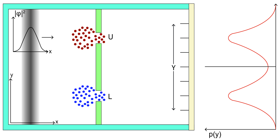
Figure 6: A qualitative representation of the probability $p(Y)$ for the observer and detector to arrive in the position interval $Y$ on the end screen. Because there is a record of which slit the system passed through, the set of histories decoheres, and the probability $p(Y)$ is the sum of the probabilities to go through the upper slit and arrive at $Y$ and the lower slit and arrive at $Y$. The result is not an interference pattern.

III.5 Records

This set of histories decoheres because a record of which slit the observer passed through is created in the state of the detector. This association between records and decoherence is a very general one and a fundamental property of DH. Decoherence implies the existence of records somewhere in the closed system although they may not be in a form that is accessible or useful to us. Conversely the existence of records of histories implies their decoherence as in this example. Indeed in realistic situations many records of the same history will be created (e.g. RZZ13 ).

Note that the set of histories decoheres whether or not the observer looks at the state of excitation. The states $\chi_{1}$ and $\chi_{2}$ are still orthogonal and (3.11) still holds.

The association of decoherence and records has been beautifully demonstrated in the experiment of Hackermüller et al hotbucky : A heated buckyball ($C_{60}$) is passed through a Talbot-Lau interferometer exhibiting a quantum interference pattern. As the temperature is increased the interference pattern dissappears when a temperature is reached where the wavelength of the radiation is short enough that it would contain a record about which slit the buckyball passed through. That is the creation of a record by emission in contrast to the creation by absorption in this toy model. But both bear out the idea that what histories that decohere are histories that are recorded.

III.6 Coarse-grained Histories

The set of histories $\{Y,S\}$ illustrated in Figure 5 is coarse grained. The position of the observer is followed only at two times $t_{S}$ and $t_{D}$ and not at all times. And these positions are not followed to arbitrary accuracy but only to the widths of the slits and of the intervals $Y$. The positions in between are unspecified — a coarse-grained description of the histories. Specifying only the interval of arrival $Y$ at the farther screen would be a coarser-grained description. Specifying more details of the path taken in between would be a finer-grained description. A coarse graining of a decoherent set like $\{Y,S\}$ is again decoherent. But fine-graining risks losing decoherence. Some coarse graining is essential for decoherence. A completely fine grained description would not decohere.

IV Third Person and First Person

In the quantum mechanics of a closed system like TSMU it is useful to distinguish between two kinds of description of the system and correspondingly two kinds of probabilities HS09 ; HH15b .

Third Person Descriptions and Probabilities: Descriptions of what the universe contains and how that evolves — histories of what occurs. Since observers are physical subsystems within the closed system, third person descriptions include a description of the histories of what observers see and how they behave. All of the previous discussion has been about third person histories of one observer and its detector — which slit it goes through, how the detector was excited, where it arrives at the screen, etc. The probabilities for these third person histories are called third person probabilities. They are what is supplied directly by the quantum state of the system and the dynamics. Examples are the probabilities $p(Y,S)$ in (3.8).

First Person Descriptions and Probabilities: Suppose that TSMU is our universe and we are the observer in it. We are interested in the first person probabilities for what we observe — what wavelength radiation we detect, which $Y$ we arrive at etc. Since we are a physical system within the universe first person probabilities can be derived from the third person probabilities for its histories. We don’t observe whole four-dimensional histories, but rather limited features of the universe from an observing situation that is localized in space and time. The first person probabilities for what we observe are necessarily conditioned on the data ${\cal D}$ describing that observational situation including the information about when the observation was made. The first person probability for an observable $\cal O$ is

$$p^{(1p)}({\cal O})=p({\cal O}|{\cal D}).$$ (4.1)

Here is an example: Our detector makes a transition to level $1$ at time $t_{S}$. We then know that we have just passed through the upper slit $U$. That is the data ${\cal D}$. Given that data what do we predict for the probability that we will arrive at position $Y$ on the screen? This is the first person probability

$$p^{(1p)}(Y)=p(Y|U)\equiv p(Y,U)/p(U).$$ (4.2)

Using (3.8) this is

$$p^{(1p)}(Y)=\frac{||\ |\Psi_{YU}(t_{D})\rangle||^{2}}{||\ |\Psi_{U}(t_{D})\rangle||^{2}}.$$ (4.3)

This distribution looks like the top part of the graph of $p(Y)$ vs. $Y$ in Figure 6 but renormalized so that the total probability for some $Y$ is unity.

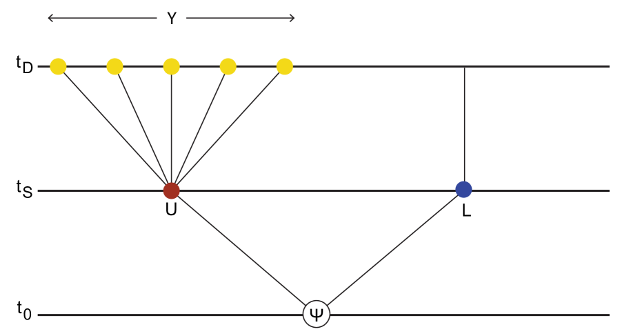
Figure 7: There are different third person descriptions of TSMU at different levels of coarse graining. Suppose at time $t_{S}$ our detector shows we went through the upper slit $U$. We want to predict where we will hit screen a the later time $t_{S}$. We could calculate using the set in Figure 5, but it would be inefficient because that also describes what would have happened if we went through the lower slit. A better set of alternative histories of TSMU is the one shown above that follows which $Y$ is reached only if we go through the upper slit. That is a coarser grained set than the one in Figure 5.

To evaluate (4.3) for $p(Y|U)$ its obviously not necessary to compute the probability of which $Y$ would have been arrived at if we had gone through the lower slit. We only need a set of histories that follows our future observations and ignores (coarse grains) over features of TSMU that are irrelevant for that. Figure 7 shows an example.

The branch wave functions of the histories in Figure 7 are (cf. (3.6))

$$\Psi_{YU}(x,y,m,t_{D}) =P_{Y}\psi_{U}(y,t_{D})\phi(x,t_{D})\delta_{m1},$$ (4.4a)

$$\Psi_{L}(x,y,m,t_{D}) =\psi_{U}(y,t_{D})\phi(x,t_{D})\delta_{m2}.$$ (4.4b)

These are decoherent because of the orthogonality of the $P_{Y}$ and the $\chi$’s.

V Some Frequently Asked Questions

Imagine that we are the observer in TSMU. A number of questions arise about quantum mechanics in this context. Many of these FAQ’s are not clearly defined. We mostly focus on FAQ’s that can be reformulated so that they are answered by appropriate quantum probabilities.

• Are we living in a superposition? Yes. Any state can be expressed as a superposition of other states for example by using a basis. This FAQ is therefore not precisely defined. Probably the question of interest to many is rather whether the state is a superposition of different histories that each can be ‘classically described’ and are ‘macroscopically distinct’. In TSMU after the time $t_{S}$ the state of the universe has evolved to the superposition of the two branches in (3.4). Each of these can described in classical terms and each could be said to constructed from alternatives that are ‘macroscopically distinct’. As the observer in the box, we are living in such a superposition. Schrödinger’s cat also lives in a superposition.

• If we are living in a superposition why arn’t we smeared out? The probability for the observer to be in two places at once is zero because the operators vanish that would represent this kind of situation. For example (3.7) shows that the wave function of the universe is in a superposition of different arrival intervals $Y$. But since $P_{Y}P_{Y^{\prime}}=0$ for $Y\neq Y^{\prime}$ (3.5) it predicts zero probabilities for the observer to be in two intervals at once. It’s the same for the slits.

• If we are living in a superposition why don’t we see a superposition or feel superposed? The detector could be part of the observer’s brain. Registrations of the detector then model a physical realization of ‘see’ and ‘feel’. We only feel going though the upper slit or alternatively feel going through the lower slit even though the quantum state is a superposition of the two. These are exclusive alternatives. The reason we don’t see the superposition is that we are not somehow outside the universe observing whether its state is a superposition of terms. We are inside the universe participating in one of the terms of the superposition.

• Does TSMU model a measurement?: Yes. There is no precise definition of ‘measurement’ in textbook (Copenhagen) quantum mechanics or in DH. But the author would informally characterize the excitation of the detector by the radiation near the slits as ‘a measurement situation’. A variable — the wavelength of the radiation — becomes correlated with an excited state of the detector that can be read by the observer. Certainly TSMU has many similarities with classic measurement models LB39 for instance the one in Figure 2. But it also differs from these models in that what is measured is not fixed, but rather determined by the quantum accident of which slit the observer passed through. Specific measurement situations can be described in DH, and their outcomes predicted, but a precise general notion of measurement is not needed for DH’s formulation.

• Do the predictions of DH differ from those of textbook quantum mechanics. Yes and No. Textbook quantum theory predicts the probabilities for the outcomes of measurements carried out by one subsystem of the universe on another. DH will predict the same probabilities to an excellent approximation. In TSMU DH would yield the same probabilities for the detector’s measurements of the radiation. But DH also predicts probabilities for which measurements are carried out where, and for the motion and fate of the observer — alternatives not considered by textbook quantum theory. Textbook quantum theory is not an alternative to DH but rather contained within it as an approximation appropriate for measurement situations.

• Would anthropic reasoning modify the predictions of TSMU?   No. Anthropic reasoning is automatic in DH through the first person probabilities for observation (Section IV) HH15b . Suppose that the radiation at the upper slit were intense enough to kill the observer. The third person probabilities for the histories $(Y,S)$ of the motion of the observer and the registration of the detector would be unchanged. But the first person probabilities for our observations would be affected assuming that the data ${\cal D}$ contained information that we are alive at the farther screen. The first person probability would be unity that we passed through the lower slit. There is zero first person probability to observe the red radiation which is where we cannot exist.

• Is the quantum state of the universe ever reduced?: No. In Section IV we derived the first person probability $p(Y|{\cal D})$ to arrive at an interval $Y$ on the far screen given data ${\cal D}$ about the detector registration. Suppose these data imply that we passed through the upper slit $U$. Equation (4.3) for this probability can be rewritten as

  $$p(Y|U)=||P_{Y}{\sf U}(t_{D},t_{S})|\Psi_{U}(t_{S})\rangle||^{2}$$ (5.1a)

  where

  $$|\Psi_{U}(t_{S})\rangle\equiv\frac{P_{U}|\Psi(t_{S})\rangle}{||P_{U}|\Psi(t_{S})\rangle||}.$$ (5.1b)

  and ${\sf U}(t_{D},t_{S})$ represents unitary evolution from $t_{S}$ to $t_{D}$ by the Schrödinger equation. Superficially the formulae (5.1) are like those in text book quantum mechanics describing the reduction of the state of a subsystem that occurs when the subsystem undergoes an ‘ideal’ measurement by another subsystem outside it. This was von Neumann’s second law of evolutionvNeu32 . But this resemblance is misleading. The states and operators in these equations are not of a subsystem of the universe being measured, but rather of the whole thing. The Hilbert space includes both what is observed and the system observing it. In the quantum mechanics of the universe there is no ‘other measuring system’ and no ‘second law of evolution’. Eq (5.1b) is not some mysterious feature of a measurement process. Rather it is but a step in the construction of conditional probabilities. It is no different from the ‘reduction’ that occurs in horse racing when a particular horse wins and the probabilities for further races which are conditioned on that event become relevant.

• Does some physical process cause the wave function to branch? No. The branching structure in Figure 5 is a choice of how to describe what goes on in TSMU. Many other descriptions are possible leading to different branching structures. Consider for example the set of histories where only $Y$ is specified and the question of which slit we go through ignored. Then there would be no branching at $t_{S}$. Or consider the set of histories in Figure 7 where there is no branching after going through the lower slit. DH does not prefer one decoherent set of histories over any other. All are in principle available to be used by us in the process of prediction although some will be more useful to human observers than others.

• Is coarse-graining necessary? Yes. Some coarse graining is necessary for decoherence except in trivial cases. Realistic mechanisms of decoherence involve coarse graining. In the classic example of Joos and Zeh JZ85 the histories of the positions of a mm size dust grain deep in intergalactic space decohere because of the vast number of CMB photons that scatter from it every second. A decoherent set of histories follows the positions of the dust grain and ignores (coarse grain over) the photons. More generally ‘environmental decoherence’ results from separating a closed system into a subsystem and an ‘environment’ and then coarse graining over its environment (e.g. GH13 ). It is a remarkable fact that in the quantum mechanics of closed systems some information must be sacrificed in order to have interesting probabilities at all.

VI Quantum Cosmology

It is an inescapable inference from the physics of the last century that we live in a quantum mechanical universe. We perhaps have little evidence of peculiarly quantum mechanical phenomena on large and even familiar scales, but there is no evidence that the phenomena that we do see cannot be described in quantum mechanical terms and explained by quantum mechanical laws. If this inference is correct, then there must be a description of the universe as a whole and everything in it in quantum mechanical terms. The nature of this description and its predictions for observations are the subject of quantum cosmology.

The two-slit universe of this paper is a toy model to illustrate a few aspects of realistic quantum cosmology. We now describe some of the connections between the model and the ongoing program of quantum cosmology.

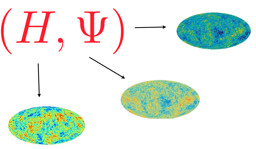
Figure 8: There are two theoretical inputs to the process of prediction in quantum cosmology. First, there is a theory of dynamics like string theory denoted here by $H$. Second is the quantum state of the universe denoted here by $\Psi$. From these third person probabilities for the individual members decoherent sets of alternative histories of the universe can be derived. From these and data describing our observational situation, first person probabilities predicting the results our observations can be calculated. These include predictions for what CMB maps we will observe.

Theoretical Inputs: Cosmology requires a generalization of usual DH to include spacetime geometry as a quantum mechanical variable Har95c . The basic theoretical inputs are a theory of dynamics including spacetime $H$– say some version of string theory — and a theory of the quantum state of the universe $\Psi$ — say Hawking’s no-boundary wave function of the universe HH83 .

Histories: Our observations of the large scale universe are mostly of properties of its classical history. The expansion, the amount of inflation, the formation of the fluctuations we see in the cosmic wave background radiation (CMB), and in the large scale distribution of galaxies today, are all properties of that classical history. Quantum cosmology aims to predict probabilities for these properties by deriving probabilities for alternative classical histories from $(H,\Psi)$ as emphasized in Figure 8.

But classical behavior is not a given in DH. It s a matter of the quantum probabilities of decoherent sets of appropriately coarse grained histories of geometry and field Har10 . A system behaves classically when the probabilities are high for histories that exhibit correlations in time by classical deterministic laws such as the Einstein equation. Classical behavior is not built into the quantum mechanics of closed systems as it was in Copenhagen theory but rather an emergent feature of the probabilities supplied by $(H,\Psi)$.

Observers and Observations: Observers and their apparatus are physical systems within the universe with only a probability to have evolved in any region of spacetime and, in a very large universe, a probability to be replicated in many regions. In TSMU the single observer (us) and detector are physical systems within the universe assumed to exist with unit probability.

3rd and 1st Person Probabilities: In quantum cosmology the theory $(H,\Psi)$ predicts third person probabilities for the history of the universe that occurs. From these probabilities for what we will observe can be predicted. In very large universes the histories most probable to occur may not be the histories that are most probable to be observed HH15b . The branch dependent adaptive coarse grainings discussed briefly in Section IV are essential for cosmology. Our observations of the universe are limited — highly coarse grained. The universe is vast. We can most efficiently calculate the prediction of theory for the outcomes of our observations by using sets of histories that follow what is observed and coarse grain over features of the universe that do not affect these observations (e.g. HHH10b ; HH15a ).

Living in a Superposition: Just like (3.7) of TSMU the quantum state of the universe is a superposition of the branch state vectors for any decoherent set of alternative classical histories. Therefore, just like the observer in TSMU, you and I are living in a superposition. We are all Schrödinger cats in Hawking’s wave function of the universe.

Acknowledgments: The author has had the benefit of discussions with a great many scientists on the work that underlies this paper. The cited papers have those acknowledgments. However, his collaborators on the those papers over a long period of time should be thanked. They are Murray Gell-Mann, Stephen Hawking, Thomas Hertog, and Mark Srednicki. Thanks are due to Mark Srednicki for critical readings of the essay and to Simon Saunders for a careful reading of the text. The work was supported in part by the US NSF grant PHY15-04541.

References

- (1) The Feynman Lectures on Physics vol 3, http://www.feynmanlectures.caltech.edu .
- (2) R.B. Griffiths, Consistent Quantum Theory, Cambridge University Press, Cambridge, UK (2002).
- (3) R. Omnès, Interpretation of Quantum Mechanics, Princeton University Press, Princeton (1994).
- (4) M. Gell-Mann and J.B. Hartle, Quantum Mechanics in the Light of Quantum Cosmology, in Complexity, Entropy, and the Physics of Information, SFI Studies in the Sciences of Complexity, Vol. VIII, ed. by W. Zurek, Addison Wesley, Reading, MA (1990).
- (5) M. Gell-Mann, The Quark and the Jaguar, W.H.. Freeman New York (1994).
- (6) P.C. Hohenberg, An introduction to consistent quantum theory, Rev. Mod. Phys. , 82 2835-2844 (2010).
- (7) The author’s papers on quantum mechanics and quantum cosmology are collected together with some commentary at http://web.physics.ucsb.edu/~quniverse. (Still under construction.)
- (8) J.B. Hartle, The Quantum Mechanics of Closed Systems, in Directions in General Relativity, Volume 1, ed. by B.-L. Hu, M.P. Ryan, and C.V. Vishveshwara, Cambridge University Press, Cambridge (1993), arXiv: gr-qc/9210006.
- (9) H. Everett III, Relative State formulation of Quantum Mechanics, Rev. Mod. Phys, 29, 454 (1957).
- (10) A Tonomura, J. Endo, T. Matsuda, T. Kawasaki, and H. Ezawa, Demonstration of Single Electron Build-Up of an Interference Pattern, Am. J. Phys. 57, 117 (1989).
- (11) M. Arndt, L. Hackermüller, K. Hornberger, and A. Zeilinger, Coherence and Decoherence Experiments with Fullerenes in Decoherence, Entanglement and Information Protection in Complex Quantum Systems, ed. by W.M. Akulin et. al., (Springer, 2005).
- (12) L. Hackermüller, K. Hornberger, B. Brezgus, A. Zeilinger, and M. Arndt, Decoherence of matter waves by thermal emission of radiation, Nature, 427, 711 (2004).
- (13) T. Juffmann, A. Milic, M. Müllerritsch, et al., Real-time single-molecule imaging of quantum interference, Nature Nanotechnology, 7, 297 (2012).
- (14) J. R. Friedman, V. Patel, W. Chen, S. Tolpygo, and J. Leukens, Quantum Superposition of Distinct Macroscopic States, Nature, 406 43 (2000).
- (15) A.J. Leggett and A. Garg, Quantum Mechanics vs. Macroscopic Realism: Is the Flux there when Nobody Looks?, Phys. Rev. Letters 54, 857 (1985).
- (16) R. Penrose, On Gravity’s Role in State Vector Reduction, Gen. Rel. Grav. 28, 581, (1996).
- (17) C. J. Riedel, W. Zurek and M. Zwolak, The Objective Past of a Quantum Universe, Pt. 1 Redundant Records of Consistent Histories, arXiv:1312.0331.
- (18) J.B. Hartle, The Reduction of the State Vector and Limitations on Measurement in the Quantum Mechanics of Closed Systems, in Directions in General Relativity, Volume 2, ed. by B.-L. Hu and T.A. Jacobson, Cambridge University Press, Cambridge (1993); arXiv:gr-qc/9301011.
- (19) M. Srednicki and J.B. Hartle, Science in a Very Large Universe, Phys. Rev. D, 81, 123524 (2010), arXiv:0906.0042, The Xerographic Distribution: Scientific Reasoning in a Large Universe, arXiv:1004.3816.
- (20) J. Hartle and T. Hertog, The Observer Strikes Back, arXiv:1503.07205.
- (21) S.W. Hawking and T. Hertog, Populating the Landscape: A Top Down Approach, Phys. Rev. D 73, 123527 (2006), arXiv:hep-th/0602091.
- (22) M. Gell-Mann and J. Hartle, Adaptive Coarse Graining, Environments, Strong Decoherence, and Quasiclassical Realms, Phys. Rev. A 89, 052125 (2014); arXiv:1312.7454.
- (23) J.B. Hartle, Quantum Physics and Human Language, J. Phys. A: Math. Theor., 40, 3101-3121 (2007), arXiv:quant-ph/0610131.
- (24) F. London and E. Bauer, La théorie de l’observation en mécanique quantique, Hermann, Paris (1939).
- (25) J. von Neumann Mathematische Grundlagen der Quantenmechanik, J. Springer, Berlin (1932). [English trans. Mathematical Foundations of Quantum Mechanics, Princeton University Press, Princeton. (1955)].
- (26) E. Joos and H.D. Zeh, The emergence of classical properties through interaction with the environment, Zeit. Phys. B, 59, 223 (1985).
- (27) J.B. Hartle, Spacetime Quantum Mechanics and the Quantum Mechanics of Spacetime in Gravitation and Quantizations, Proceedings of the 1992 Les Houches Summer School, ed. by B. Julia and J. Zinn-Justin, (North Holland, Amsterdam, 1995); arXiv:gr-qc/9304006.
- (28) J. B. Hartle and S. W. Hawking, The Wave Function of the Universe, Phys. Rev. D 28, 2960-2975 (1983), S.W. Hawking, The Quantum State of the Universe, Nucl. Phys. B, 239, 257-276 (1984).
- (29) J.B. Hartle, The quasiclassical realms of this quantum universe, arXiv:0806.3776. A slightly shorter version is published in Many Worlds? edited by S. Saunders, J. Barrett, A. Kent, and D. Wallace (Oxford University Press, Oxford, 2010), the longer version was published in Foundations of Physics, 41, 982 (2011).
- (30) J. B. Hartle, S. W. Hawking, T. Hertog, Local Observation in Eternal Inflation, Phys. Rev. Lett. 106, 141302 (2011), arXiv:1009.252.
- (31) J.B. Hartle and T. Hertog, One bubble to rule them all, arXiv:1604.03580.