Nonrelativistic Banks–Casher relation and random matrix theory for multi-component fermionic superfluids

Abstract

We apply QCD-inspired techniques to study nonrelativistic $N$-component degenerate fermions with attractive interactions. By analyzing the singular-value spectrum of the fermion matrix in the Lagrangian, we derive several exact relations that characterize the spontaneous symmetry breaking $\text{U}(1)\times\text{SU}(N)\to\text{Sp}(N)$ through bifermion condensates. These are nonrelativistic analogues of the Banks–Casher relation and the Smilga–Stern relation in QCD. Non-local order parameters are also introduced and their spectral representations are derived, from which a nontrivial constraint on the phase diagram is obtained. The effective theory of soft collective excitations is derived and its equivalence to random matrix theory is demonstrated in the $\varepsilon$-regime. We numerically confirm the above analytical predictions in Monte Carlo simulations.

I Introduction

Spontaneous symmetry breaking is a universal concept across broad fields of physics. The Bose–Einstein condensation of atoms is a marked example of quantum phenomena accessible in laboratory experiments Kapitza (1938); Osheroff et al. (1972); Anderson et al. (1995); Davis et al. (1995). Superconductivity of electrons plays an essential role in condensed matter physics and furnishes diverse technological applications Bardeen et al. (1957). Chiral symmetry breaking in quantum chromodynamics (QCD) is a dominant mechanism for mass generation in our universe Nambu (1960); Nambu and Jona-Lasinio (1961a, b). The masses of elementary particles are generated by the Higgs mechanism Higgs (1964a); Englert and Brout (1964); Higgs (1964b).

Spontaneous symmetry breaking is driven by quantum effects. For its exact derivation, the full information of a quantum many-body vacuum is necessary, but it is extremely difficult to obtain. To tackle this difficult problem, many theoretical approaches have been developed in each field. Although they are formulated in different ways among different fields, the underlying physics must be common and an approach that proved successful in one field is expected to be applicable to another field. Such an interdisciplinary endeavor is of vital importance to grasp the true nature of a universal phenomenon.

The target of this paper is spontaneous symmetry breaking in nonrelativistic multi-component degenerate fermions. This occurs in a variety of physical situations in nature. In nuclear physics, an atomic nucleus is composed of protons and neutrons with two spin states, entailing an approximate spin-isospin symmetry Gaponov et al. (1996). In ultracold atomic systems, $\text{SU}(N)$-symmetric ultracold Fermi gases have been experimentally realized Taie et al. (2010). The $\text{SU}(N)$ Hubbard model on a lattice has also attracted attention Honerkamp and Hofstetter (2004a); Taie et al. (2012). We refer to Wu et al. (2003); Honerkamp and Hofstetter (2004b); Veillette et al. (2007); Cherng et al. (2007); Gorshkov et al. (2009); Cazalilla et al. (2009); Szirmai and Lewenstein (2010); Yip (2011); hsuan Hung et al. (2011); Yip et al. (2014); Zhang et al. (2014) for a partial list of works addressing the novel physics of multi-component Fermi gases, and Cazalilla and Rey (2014) for a recent review.

In this work, we apply analytical tools established in the study of spontaneous chiral symmetry breaking in QCD to interacting nonrelativistic fermions with an even number of components. As in QCD, we analyze the eigenvalues (more precisely, the singular values) of the fermion matrix in the Lagrangian formalism. The structure of the spectrum reflects realization of global symmetries in the ground state. We derive some exact relations between the spectrum and symmetry breaking, including the nonrelativistic counterparts of the Banks–Casher relation (Sec. II) and the Smilga–Stern relation (Sec. IV), both of which are well established in studies of the Dirac operator in QCD. In addition, by relating two-point correlation functions of fermion bilinears to the singular-value spectrum, we show in Sec. III that if $\text{U}(1)$ symmetry is spontaneously broken, then $\text{SU}(N)$ symmetry must be broken down to $\text{Sp}(N)$, and vice versa, in $N$-component fermions. A salient feature of the Dirac spectrum in QCD is that it obeys random matrix theory (RMT) in a finite-volume regime called microscopic domain (or $\varepsilon$-regime). In Sec. V we derive the effective theory of soft collective excitations for nonrelativistic multi-component fermions, and identify the correspondence between the singular-value spectrum and RMT. We verify these analytical predictions by path-integral Monte Carlo simulations of nonrelativistic fermions on a lattice, utilizing powerful techniques developed in lattice QCD (Sec. VI). In Appendixes, a few analytical derivations are given for completeness.

II Banks–Casher-type relation

Our main interest is in $N$-component degenerate fermions with $s$-wave contact interactions with $\text{U}(N)$-symmetric theory, where $N=2,4,6,\dots$ is assumed to be even. We will work in $D$-dimensional space with $D=2$ and $3$. The action in the imaginary-time formalism is given (in the unit $\hbar=1$) by

$$S =\int_{x}\left[\sum_{i=1}^{N}\psi_{i}^{*}\left(\partial_{\tau}-\frac{\nabla^{2}}{2m}-\mu\right)\psi_{i}+\frac{c}{2}\,\bigg{(}\sum_{i=1}^{N}\psi^{*}_{i}\psi_{i}\bigg{)}^{2}\right]$$ (1)

with $\int_{x}\equiv\int_{0}^{\beta}\mathrm{d}\tau\int\mathrm{d}^{D}\mathbf{x}$. The coupling $c<0$ ($c>0$) represents an attractive (repulsive) interaction, respectively. The inverse temperature $\beta=1/k_{B}T$ is arbitrary at this stage. The partition function is given by the path integral $Z=\int\mathcal{D}\psi^{*}\mathcal{D}\psi\,\exp(-S)$. At $N=2$, Eq. (1) is reduced to the conventional spin-$1/2$ Fermi gas with $\text{U}(1)\times\text{SU}(2)$ symmetry.

From here on, we concentrate on the attractive interaction and let $g\equiv-c>0$. By means of a Hubbard–Stratonovich transformation, one obtains $Z=\int\mathcal{D}\psi^{*}\mathcal{D}\psi\mathcal{D}\phi\,\exp(-S^{\prime})$ with

$$S^{\prime} =\int_{x}\left[\sum_{i=1}^{N}\psi_{i}^{*}\left(\partial_{\tau}-\frac{\nabla^{2}}{2m}-\mu-g\phi\right)\psi_{i}+\frac{g}{2}\phi^{2}\right]\,,$$ (2)

where $\phi(x)$ is a real bosonic auxiliary field. Now $S^{\prime}$ is bilinear in fermion fields.

If the system develops a fermion pair condensate $\left\langle\psi_{i}\psi_{j}\right\rangle$, it breaks $\text{U}(N)$ symmetry spontaneously. To extract the condensate, it is useful to add the following source term to the action

$$\delta S=-\frac{j}{2}\int_{x}\left(\psi_{i}I_{ij}\psi_{j}+\text{h.c.}\right)\,,$$ (3)

with $I\equiv\begin{pmatrix}0&1\\ -1&0\end{pmatrix}\otimes\mathbb{1}_{N/2}$ . This term breaks $\text{U}(N)$ symmetry down to the unitary symplectic group defined by

$$\text{Sp}(N) =\left\{u\in\text{SU}(N)\,|\,u^{T}Iu=I\right\}\,.$$ (4)

We introduce the source term (3) with $j>0$, and then let $j\to 0$ in the end of calculations. A nonzero condensate in the $j\to 0$ limit signals spontaneous $\text{U}(N)$ symmetry breaking.

Combining Eq. (3) with Eq. (2) and going to the Nambu–Gor’kov representation, one finds

$$S^{\prime}+\delta S$$

$$= \int_{x}\bigg{[}\sum_{k=1}^{N/2}\big{(}\begin{array}[]{cc}\psi^{*}_{2k-1}&\psi_{2k}\end{array}\big{)}\begin{pmatrix}W&j\\ j&-W^{\dagger}\end{pmatrix}\begin{pmatrix}\psi_{2k-1}\\ \psi_{2k}^{*}\end{pmatrix}+\frac{g}{2}\phi^{2}\bigg{]}$$ (6)

with

$$W\equiv\partial_{\tau}-\frac{\nabla^{2}}{2m}-\mu-g\phi\,.$$ (7)

The next step is to integrate out fermions, with the result

$$Z(j) =\int\mathcal{D}\phi~{}{\det}^{N/2}\begin{pmatrix}W&j\\ j&-W^{\dagger}\end{pmatrix}\exp\left(-\frac{g}{2}\int_{x}~{}\phi^{2}\right)$$

$$=\int\mathcal{D}\phi~{}{\det}^{N/2}\left(j^{2}+WW^{\dagger}\right)\exp\left(-\frac{g}{2}\int_{x}~{}\phi^{2}\right)\,.$$ (8)

This form manifestly shows that the path-integral measure is positive definite so that this theory can be simulated with standard Monte Carlo methods. We warn that this is no longer true if $N$ is odd or if the interaction is repulsive.

It is now straightforward to find the fermion condensate by taking the derivative with $j$,

$$\frac{1}{2}\left\langle\psi^{T}I\psi+\text{h.c.}\right\rangle =\lim_{V\to\infty}\frac{1}{\beta V}\frac{\mathrm{d}}{\mathrm{d}j}\log Z(j)$$

$$=\frac{N}{2}\lim_{V\to\infty}\frac{1}{\beta V}\bigg{\langle}\sum_{n}\frac{2j}{j^{2}+\Lambda_{n}^{2}}\bigg{\rangle}$$

$$=\frac{N}{2}\int_{0}^{\infty}\!\!\!\mathrm{d}\Lambda~{}\frac{2j}{j^{2}+\Lambda^{2}}R_{1}(\Lambda),$$ (9)

where $V$ is the spatial volume and $\Lambda_{n}\geq 0$ are square roots of the eigenvalues of $WW^{\dagger}$ (i.e., the singular values of $W$). The spectral density (or one-point function), $R_{1}(\Lambda)$, is defined for $\Lambda\geq 0$ as

$$R_{1}(\Lambda) \equiv\lim_{V\to\infty}\frac{1}{\beta V}\bigg{\langle}\sum_{n}\delta(\Lambda-\Lambda_{n})\bigg{\rangle}$$ (10)

where the average $\left\langle\cdots\right\rangle$ is taken with respect to the measure (8). By taking the limit $j\to 0$, we arrive at

$$\lim_{j\to+0}\frac{1}{2}\left\langle\psi^{T}I\psi+\text{h.c.}\right\rangle=\frac{N}{2}\pi\lim_{j\to+0}R_{1}(0).$$ (11)

This relation, linking the density of small singular values of $W$ to spontaneous symmetry breaking $\text{U}(1)\times\text{SU}(N)\to\text{Sp}(N)$, is the main result of this section. This is a generalization of the celebrated Banks–Casher relation for gauge theories Banks and Casher (1980) to nonrelativistic fermions. Several remarks are in order.

• As is clear from the derivation above, the new relation (11) holds both in the normal phase and in the superfluid phase. The temperature, chemical potential and the interaction strength are arbitrary.

• The action (1) based on the $s$-wave contact interaction has an intrinsic short-distance cutoff scale (i.e., the effective range of the inter-particle potential). This implies that it is not physically meaningful to integrate over $\Lambda$ up to infinity in Eq. (9) beyond the short-distance cutoff. However, a more elaborate treatment of the integral would not change the final formula (11) because all contributions to Eq. (9) from regions away from the origin will eventually drop out in the limit $j\to 0$. Thus Eq. (11) holds irrespective of the detailed short-distance physics.

• We stress that the positivity of the measure is essential for the derivation of Eq. (11). If the measure becomes negative or complex, the spectral density tends to be a violently oscillating function that has no smooth thermodynamic limit Akemann et al. (2005); Osborn et al. (2005); Kanazawa et al. (2011); Kanazawa and Wettig (2014); Verbaarschot and Wettig (2014), so that the last step from Eq. (9) to Eq. (11) replacing $\frac{2j}{j^{2}+\Lambda^{2}}$ with $2\pi\delta(\Lambda)$ is invalidated. This suggests that this kind of an exact formula will not exist in a spin-imbalanced Fermi gas, even though the condensate itself may exist.

• In the free limit $g\to 0$, one can compute $R_{1}(\Lambda)$ analytically, as outlined in Appendix A. In $D=3$ dimensions at $T=0$, we find

  $$R_{1}(\Lambda)\propto\Lambda^{3/2}$$ (12)

  for $\mu=0$ and

  $$R_{1}(\Lambda)\propto\sqrt{\mu}\,\Lambda$$ (13)

  for $\mu\gg\Lambda>0$. In either case $R_{1}(0)=0$ gives a vanishing condensate, but it is worthwhile to note that the density of small eigenvalues is substantially enhanced for $\mu>0$ as compared to $\mu=0$. This means that a positive chemical potential (or the presence of a Fermi surface) acts as a catalyst of spontaneous symmetry breaking. Analogous phenomena occur in the singular-value spectrum of the Dirac operator in dense QCD-like theories Kanazawa et al. (2011) and the Dirac spectrum of QCD in an external magnetic field Shushpanov and Smilga (1997); in both cases the spectral density near the origin is enhanced from $\sim\Lambda^{3}$ to $\sim\Lambda$.

• While the above derivation focuses on the $\text{Sp}(N)$-symmetric condensate $\left\langle\psi^{T}I\psi\right\rangle$, one can also consider $\left\langle\psi^{T}IT^{A}\psi\right\rangle$ and $\left\langle\psi^{\dagger}t^{a}\psi\right\rangle$, where Peskin (1980); Kogut et al. (2000)

  • $\{T^{A}\}\cdots$$N(N-1)/2-1$ generators of the coset space $\text{SU}(N)/\text{Sp}(N)$, normalized as $\operatorname{tr}(T^{A}T^{B})=\frac{1}{2}\delta^{AB}$. $(T^{A})^{T}I=IT^{A}$ holds.

  • $\{t^{a}\}\cdots$$N(N+1)/2$ generators of $\text{Sp}(N)$, normalized as $\operatorname{tr}(t^{a}t^{b})=\frac{1}{2}\delta^{ab}$. $(t^{a})^{T}I=-It^{a}$ holds.

  The former condensate transforms in the rank-2 antisymmetric tensor representation of $\text{Sp}(N)$, while the latter in the adjoint representation of $\text{Sp}(N)$. From the Vafa-Witten theorem Vafa and Witten (1984); Kosower (1984), one can show $\left\langle\psi^{T}IT^{A}\psi\right\rangle=\left\langle\psi^{\dagger}t^{a}\psi\right\rangle=0$ for any $j\neq 0$. This argument assures that $\text{Sp}(N)$ symmetry is unbroken for any $j\neq 0$. Namely, $\text{Sp}(N)$-symmetric states have lower free energy than $\text{Sp}(N)$-breaking states at $j\neq 0$. Then, if any $\text{Sp}(N)$-breaking states are degenerate with $\text{Sp}(N)$-symmetric states in the $j\to 0$ limit, $\text{Sp}(N)$ symmetry could be spontaneously broken. We will assume that $\text{Sp}(N)$ is not spontaneously broken throughout the remainder of this paper.

III $\text{U}(1)$ versus $\text{SU}(N)$ symmetry

While $\left\langle\psi^{T}I\psi\right\rangle\neq 0$ signals spontaneous breakdown of both $\text{U}(1)$ and $\text{SU}(N)$ for even $N\geq 4$, one can in principle also imagine a phase where either $\text{U}(1)$ or $\text{SU}(N)$ is broken but the other is unbroken. Taking such intermediate phases into account leads us to three distinct phase diagrams sketched in Fig. 1.

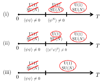
Figure 1: Classification of possible finite-temperature phase diagrams for even $N\geq 4$.

In cases (i) and (ii) there appear phases with partial symmetry breaking, while in case (iii) $\text{U}(1)$ and $\text{SU}(N)$ are simultaneously restored. (Similar diagrams can be drawn for a varying interaction strength.)

In this section, we shall use spectral methods inspired by QCD to argue that such exotic intermediate phases should not arise at least for $N=4$. The key requirement in our analysis is that, to characterize phases with no bilinear condensate, one must consider higher-order condensates containing more than two fermions, as a source of symmetry breaking. We clarify the necessary and sufficient condition for the singular-value spectrum of $W$ to support such higher-order condensates in a phase with $\lim_{j\to 0}R_{1}(0)=0$.

We mention that there are ample literature on symmetry breaking driven by higher-order condensates in high-energy physics. In QCD at finite density, the breaking of $\text{U}(1)$ baryon number symmetry and chiral symmetry in color-superconducting phases is characterized by a six-quark condensate and a four-quark condensate, respectively Rajagopal and Wilczek (2000); Alford et al. (2008). Four-quark condensates also appear in the hypothetical Stern phase of QCD Stern (1998); Kogan et al. (1999); Kanazawa (2015). Non-local four-quark operators play a central role in the debate over effective restoration of the anomalous $\text{U}(1)_{A}$ symmetry at high temperature Shuryak (1994); Cohen (1996); Bernard et al. (1997); Chandrasekharan et al. (1999); Edwards et al. (2000); Kanazawa and Yamamoto (2015). Furthermore, in some inhomogeneous phases of QCD, the bilinear condensate is washed out by strong fluctuations of phonons, so the leading condensate consists of four quarks Hidaka et al. (2015) (see Radzihovsky (2011, 2012) for analogs in condensed matter physics).

Returning to the nonrelativistic $N$-component system of fermions, we define four bilinears as

$$\Pi^{0}(x) \equiv i(\psi^{T}IT^{0}\psi+\psi^{\dagger}T^{0}I\psi^{*})$$ (14a)

$$\Delta^{0}(x) \equiv\psi^{T}IT^{0}\psi-\psi^{\dagger}T^{0}I\psi^{*}$$ (14b)

$$\Pi^{A}(x) \equiv i(\psi^{T}IT^{A}\psi+\psi^{\dagger}T^{A}I\psi^{*})$$ (14c)

$$\Delta^{A}(x) \equiv\psi^{T}IT^{A}\psi-\psi^{\dagger}T^{A}I\psi^{*}$$ (14d)

where $\{T^{A}\}$ are the generators of $\text{SU}(N)/\text{Sp}(N)$ as before, and $T^{0}\equiv\mathbb{1}_{N}/\sqrt{2N}$. These operators are mixed with each other under $\text{U}(1)\times\text{SU}(N)$ transformations, as summarized in Fig. 2.

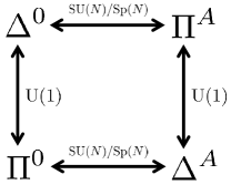
Figure 2: The four fermion bilinears that transform to each other under $\text{U}(1)$ and $\text{SU}(N)/\text{Sp}(N)$ rotations.

We define the integrated connected correlator of a field $X=\{\Pi^{0},\Delta^{0},\Pi^{A},\Delta^{A}\}$ as

$$\mathsf{C}_{X}\equiv\int_{x}\int_{y}\big{\{}\left\langle X(x)X(y)\right\rangle-\left\langle X(x)\right\rangle\left\langle X(y)\right\rangle\big{\}}\,,$$ (15)

where the averages are taken with respect to the measure (8). This is an extensive quantity and must be divided by $\beta V$ when the thermodynamic limit is taken later. The explicit forms of $\mathsf{C}_{X}$ are presented in Appendix B.

Let us introduce non-local observables that are sensitive to the realization of $\text{U}(1)$ and $\text{SU}(N)$ symmetry. Since $\Pi^{0}$ mixes with $\Delta^{A}$ under $\text{SU}(N)$ transformations [cf. Fig. 2], one must have

$$\mathsf{C}_{\Pi^{0}}=\mathsf{C}_{\Delta^{A}}$$ (16)

in the $j\to 0$ limit if $\text{SU}(N)$ is unbroken. This property prompts us to define

$$\begin{split}\omega_{\scriptscriptstyle\text{SU}(N)}&\equiv\frac{1}{\beta V}\sum_{A}(\mathsf{C}_{\Pi^{0}}-\mathsf{C}_{\Delta^{A}})\\ &=\frac{1}{\beta V}\left[\frac{N^{2}-N-2}{2}\mathsf{C}_{\Pi^{0}}-\sum_{A}\mathsf{C}_{\Delta^{A}}\right]\\ &=\frac{2(N^{2}-N-2)}{\beta V}\bigg{\langle}\!\operatorname{tr}\frac{j^{2}}{(W^{\dagger}W+j^{2})^{2}}\bigg{\rangle}\\ &=2(N^{2}-N-2)\int_{0}^{\infty}\!\!\!\mathrm{d}\Lambda\frac{j^{2}}{(\Lambda^{2}+j^{2})^{2}}R_{1}(\Lambda)\,,\end{split}$$ (17)

where formulas in Appendix B have been used repeatedly. Next, Fig. 2 shows that $\Pi^{A}$ and $\Delta^{A}$ mix with each other under $\text{U}(1)$ transformations. Hence one must have

$$\mathsf{C}_{\Pi^{A}}=\mathsf{C}_{\Delta^{A}}$$ (18)

in a phase with unbroken $\text{U}(1)$ symmetry. Let us define

$$\begin{split}\tilde{\omega}_{\scriptscriptstyle\text{U}(1)}&\equiv\frac{1}{\beta V}\sum_{A}(\mathsf{C}_{\Pi^{A}}-\mathsf{C}_{\Delta^{A}})\\ &=2(N^{2}-N-2)\int_{0}^{\infty}\!\!\!\mathrm{d}\Lambda\frac{j^{2}}{(\Lambda^{2}+j^{2})^{2}}R_{1}(\Lambda)\,.\end{split}$$ (19)

Intriguingly, this is exactly equal to Eq. (17). Hence

$$\omega_{\scriptscriptstyle\text{SU}(N)}=\tilde{\omega}_{\scriptscriptstyle\text{U}(1)}$$ (20)

follows. What is the physical meaning of this relation? Let us consider the following two cases separately.

• $N\geq 6$. Since

  $$\qquad\tilde{\omega}_{\scriptscriptstyle\text{U}(1)}\! =-\frac{2}{\beta V}\!\int_{x,y}\!\!\!\!\left\langle\psi^{T}(x)IT^{A}\psi(x)\psi^{T}(y)IT^{A}\psi(y)\right\rangle$$

  $$\quad+\text{h.c.}$$

  is a charge-4 condensate, it must vanish when $\mathbb{Z}_{N}\subset\text{SU}(N)$ with $N\geq 6$ is restored, irrespective of the $\text{U}(1)$ symmetry realization. In other words, unbroken $\text{SU}(N)$ is enough to ensure the degeneracy of $(\Pi^{0},\Delta^{0},\Pi^{A},\Delta^{A})$ even though $\text{U}(1)$ could still be broken by higher order condensates. Thus Eq. (20) does not tell us anything about the interrelation between $\text{U}(1)$ and $\text{SU}(N)$ symmetries — we only learn that the restoration of $\text{SU}(N)$ symmetry requires not only $\lim_{j\to 0}R_{1}(0)=0$ but also

  $$\lim_{j\to 0}\int_{0}^{\infty}\!\!\!\mathrm{d}\Lambda\frac{j^{2}}{(\Lambda^{2}+j^{2})^{2}}R_{1}(\Lambda)=0\,,$$ (21)

  which is a far more stringent condition than $\lim_{j\to 0}R_{1}(0)=0$.

• $N=4$. Unbroken $\text{SU}(4)$ symmetry does not imply $\tilde{\omega}_{\scriptscriptstyle\text{U}(1)}=0$, so $\tilde{\omega}_{\scriptscriptstyle\text{U}(1)}$ can now be treated as a faithful order parameter for $\text{U}(1)$ symmetry breaking. We interpret the coincidence (20) as an indication that $\text{U}(1)$ breaking goes hand-in-hand with $\text{SU}(4)$ breaking. Hence intermediate phases as depicted in Fig. 1 are not expected to arise in the phase diagram.

Since there is no obvious reason to regard the $N=4$ fermion system as exceptional, we conjecture that the simultaneous restoration of $\text{U}(1)$ and $\text{SU}(N)$ would be a generic phenomenon for $N\geq 4$. A further investigation on this issue is left for future work.

Finally we wish to analyze the possibility that both $\text{U}(1)$ and $\text{SU}(N)$ are broken by higher-order condensates despite $\left\langle\psi^{T}I\psi\right\rangle=0$. This hypothetical phase, characterized by $\lim_{j\to 0}R_{1}(0)=0$ and

$$\lim_{j\to 0}\int_{0}^{\infty}\!\!\!\mathrm{d}\Lambda\frac{j^{2}}{(\Lambda^{2}+j^{2})^{2}}R_{1}(\Lambda)>0\,,$$ (22)

is not excluded by the arguments in this section. What is the form of $R_{1}(\Lambda)$ consistent with Eq. (22)? It is readily seen that if $R_{1}(\Lambda)$ is strictly zero in the range $0\leq\Lambda\leq\lambda_{0}$ for some $\lambda_{0}>0$ (as is the case for free fermions at finite temperature), then $\omega_{\scriptscriptstyle\text{SU}(N)}=\tilde{\omega}_{\scriptscriptstyle\text{U}(1)}=\mathcal{O}(j^{2})\to 0$ and the symmetry is restored. Thus a nonzero density of eigenvalues in the infinitesimal vicinity of the origin is a necessary condition for Eq. (22). More precisely, Eq. (22) holds if $R_{1}$ has the form

$$R_{1}(\Lambda) \sim j^{\alpha}\Lambda^{1-\alpha}\qquad\text{for}\quad 0\leq\alpha\leq 1\,.$$ (23)

A somewhat puzzling instance of the behavior (23) is encountered in a free theory at $T=0$, where $R_{1}(\Lambda)\propto\Lambda$ for $\mu>0$ (see Appendix A). Our interpretation is that this is not a true symmetry breaking but rather an indication that free fermions at $\mu>0$ is on the verge of symmetry breaking. At $\mu>0$, a nonzero density of states at the Fermi surface ensures that fermion pairs condense and break symmetries spontaneously for an arbitrarily weak attractive interaction $g>0$, i.e., the Cooper instability. We believe that $\omega_{\scriptscriptstyle\text{SU}(N)}=\tilde{\omega}_{\scriptscriptstyle\text{U}(1)}\neq 0$ at $g=0$ should be seen as an extrapolation of symmetry breaking in the limit $g\to+0$. Note that they vanish as soon as we raise the temperature from zero; namely, the true many-body effect is needed to achieve $\omega_{\scriptscriptstyle\text{SU}(N)}=\tilde{\omega}_{\scriptscriptstyle\text{U}(1)}\neq 0$ at any small but nonzero $T>0$. A quite similar phenomenon is known to occur when Dirac fermions are subjected to an external magnetic field in $2+1$ dimensions: the chiral condensate assumes a nonzero value even in a free theory Gusynin et al. (1994, 1995). This deceiving condensate evaporates at any nonzero temperature Das and Hott (1996), similarly to our case.

IV Smilga–Stern-type relation

One of the defining features of superfluidity is a nonzero stiffness (helicity modulus) Fisher et al. (1973). It is important to understand how the information of the stiffness is imprinted in the spectral density $R_{1}(\Lambda)$. In this section we apply the method of low-energy effective field theory (EFT) to show that, while $\lim_{j\to 0}R_{1}(0)$ is proportional to the condensate, the slope of $\lim_{j\to 0}R_{1}(\Lambda)$ is sensitive to the phase stiffness. This is a generalization of the so-called Smilga–Stern relation Smilga and Stern (1993); Osborn et al. (1999); Toublan and Verbaarschot (1999) in QCD to nonrelativistic superfluids. Our method is applicable to even $N\geq 4$ in the phase where $\left\langle\psi^{T}I\psi\right\rangle\neq 0$. This requires $D=3$ at sufficiently low $T$ or $D=2$ at $T=0$.

EFT is a powerful method enabling a systematic description of low-energy physics based on symmetries. It can be equally applied to systems with or without Lorentz invariance, as has been theoretically demonstrated in Leutwyler (1994); Watanabe and Murayama (2012); Hidaka (2013); Takahashi and Nitta (2015); see Watanabe and Murayama (2014); Andersen et al. (2014) for a comprehensive overview of the subject. In multi-component Fermi gases with even $N\geq 4$, fermions are gapped through $s$-wave pairing and the dominant excitations at low energy are gapless Nambu–Goldstone modes originating from the symmetry breaking $\text{U}(1)\times\text{SU}(N)\to\text{Sp}(N)$. Since the construction of the effective Lagrangian in this case closely parallels previous works in two-color QCD Peskin (1980); Smilga and Verbaarschot (1995); Kogut et al. (1999, 2000); Kanazawa et al. (2009, 2011), we refer to these references for details and only recapitulate the main ideas.

The first step is to generalize the source term (3) to

$$\delta S=-\frac{1}{2}\int_{x}(\psi^{T}J\psi+\text{h.c.})$$ (24)

where

$$J =jI+\sum_{A}j_{A}IT^{A}$$ (25)

is the most general decomposition of an antisymmetric $N\times N$ matrix Kanazawa et al. (2011). Corrections to the effective action due to $J$ can be sorted out in a perturbative manner. At leading order in the number of derivatives ($\partial_{\tau}$, $\nabla$) and the external field ($J$) we obtain

$$\begin{split}\mathcal{L}_{\rm eff}&=F^{2}\!\left[\operatorname{tr}\!\left(\partial_{\tau}\Sigma^{\dagger}\partial_{\tau}\Sigma\right)+v^{2}\operatorname{tr}\!\left(\nabla_{i}\Sigma^{\dagger}\nabla_{i}\Sigma\right)\right]\\ &\quad+\frac{1}{2}\!\left[(\partial_{\tau}\phi)^{2}+\tilde{v}^{2}(\nabla_{i}\phi)^{2}\right]+\Phi\,\mathrm{Re}\operatorname{tr}(J\tilde{\Sigma})\,,\end{split}$$ (26)

which will be valid if $k_{\rm B}T$ is much lower than the gap in the single-particle excitation spectrum.

Several remarks are in order.

• The coset manifold $\text{SU}(N)/\text{Sp}(N)$ is parametrized by $\Sigma(x)=UIU^{T}=U^{2}I$ Kogut et al. (2000) with

  $$U(x) =\exp\left(i\frac{\pi^{A}(x)T^{A}}{2F}\right),$$ (27)

  where $\{\pi^{A}\}$ are the Nambu–Goldstone modes. $\Sigma$ satisfies $\Sigma^{T}=-\Sigma$ and $\Sigma^{\dagger}\Sigma=\mathbb{1}_{N}$. The coefficient of $(\partial_{\tau}\pi^{A})^{2}$ in Eq. (26) is normalized to $1/2$. $v$ denotes the velocity of the $\pi$ fields.

• The superfluid phonon is represented by $\phi(x)$, with the velocity $\tilde{v}$. In $\tilde{\Sigma}$, the phonon is coupled to $\pi$ as

  $$\tilde{\Sigma} =\Sigma\operatorname{e}^{i\phi/f}\,.$$ (28)

  In two-color QCD, $\phi(x)$ is absent because the axial $\text{U}(1)$ symmetry in QCD is violated by chiral anomaly.

• The last term in Eq. (26) containing $J$ breaks the $\text{SU}(N)$ symmetry explicitly and generates a nonzero gap (“mass”) for the Nambu–Goldstone modes. At ${}^{\forall}j_{A}=0$ we have

  $$m_{\pi}^{2}=\frac{j\Phi}{2F^{2}}\quad\text{and}\quad m_{\phi}^{2}=\frac{jN\Phi}{f^{2}}\,.$$ (29)

• Evaluating the derivative of $\log Z$ with $j$ at ${}^{\forall}j_{A}=0$ one finds

  $$\Phi =\lim_{j\to 0}\frac{1}{2N}\left\langle\psi^{T}I\psi+\text{h.c.}\right\rangle\,.$$ (30)

  Combined with our Banks–Casher-type relation (11), this means $\lim_{j\to 0}R_{1}(0)=2\Phi/\pi$. We note that $F,f,v,\tilde{v}$ and $\Phi$ all depend implicitly on $T,\mu,g$ and $N$.

• Generally, in the absence of Lorentz invariance, terms linear in the time derivative can appear in effective Lagrangians and modify dispersion relations of Nambu–Goldstone modes qualitatively Leutwyler (1994); Watanabe and Murayama (2012); Hidaka (2013). This indeed occurs in the three-component fermionic superfluids He et al. (2006); Yip (2011). However this does not occur for even $N$ Yip (2011); Cazalilla and Rey (2014); i.e., the number of Nambu–Goldstone modes is equal to that of broken generators and they all enjoy a linear dispersion. This can be argued as follows. According to Schafer et al. (2001); Watanabe and Murayama (2012); Hidaka (2013), the number of Nambu–Goldstone modes must be equal to the number of broken generators if $\left\langle[Q_{a},Q_{b}]\right\rangle=0$ for all pairs of broken generators $\{Q_{i}\}$. In the case of $N$-component fermions with even $N$, the fact that the coset $\text{SU}(N)/\text{Sp}(N)$ is a symmetric space Peskin (1980) implies that a commutator of broken generators is a linear combination of unbroken generators. Then, if there is a nonzero density of $\text{Sp}(N)$ charges in the ground state, it breaks $\text{Sp}(N)$ and contradicts the assumption of unbroken $\text{Sp}(N)$ symmetry. Hence $\left\langle[Q_{a},Q_{b}]\right\rangle=0$.

• In two-color QCD, a Wess–Zumino–Witten term proportional to $\varepsilon^{\mu\nu\rho\sigma}$ is necessary to account for the axial anomaly at the level of the chiral Lagrangian Duan et al. (2001); Lenaghan et al. (2002). The same term can emerge in our effective theory as well (in $3+1$ dimensions) at the cost of parity, but this term is fourth order in derivatives and can be safely neglected at low energy.

• Suitable extensions of Eq. (26) to the imbalanced case were thoroughly discussed in Kogut et al. (1999, 2000); Splittorff et al. (2001); Brauner (2006); Kanazawa et al. (2009) in the context of two-color QCD.

Having introduced EFT, we are in a position to compute low-energy observables. We calculate the susceptibility

$$\chi_{AB}(j) \equiv\lim_{\forall j_{A}\to 0}\lim_{V\to\infty}\frac{1}{\beta V}\frac{\partial^{2}}{\partial j_{A}\partial j_{B}}\log Z$$ (31)

from both the microscopic action and EFT. In the microscopic theory, we have

$$\chi_{AB}(j) =\frac{\delta_{AB}}{2}\int_{0}^{\infty}\!\!\!\mathrm{d}\Lambda\,\frac{\Lambda^{2}-j^{2}}{(\Lambda^{2}+j^{2})^{2}}R_{1}(\Lambda)\,.$$ (32)

On the EFT side, we find that the leading infrared singularity as $j\to 0$ is given by

$$\chi_{AB}(j) \simeq-\delta_{AB}\,\hat{\chi}\,\log j\,,$$ (33)

with

$$\hat{\chi} \equiv\frac{1}{128\pi^{2}}\frac{\Phi^{2}}{F^{4}}\bigg{[}\frac{(N-4)(N+2)}{8N}\frac{1}{v^{3}}+\frac{4}{v\tilde{v}(v+\tilde{v})}\frac{F^{2}}{f^{2}}\bigg{]}$$ (34)

at $D=3$ and $T=0$. The derivations of Eqs. (32), (33), and (34) are given in Appendix C. The infrared divergence in Eq. (33) must be accounted for by Eq. (32) as well, i.e., for small $j$

$$\int_{0}^{\infty}\!\!\!\mathrm{d}\Lambda\,\frac{\Lambda^{2}-j^{2}}{(\Lambda^{2}+j^{2})^{2}}R_{1}(\Lambda)\simeq-2\hat{\chi}\log j\,.$$ (35)

This constrains the possible form of $R_{1}(\Lambda)$. We note that the constant part of $R_{1}(\Lambda)$ does not contribute to the integral Smilga and Stern (1993), since $\int_{0}^{\infty}\mathrm{d}x\frac{x^{2}-1}{(x^{2}+1)^{2}}=0$. A logarithmic divergence could be reproduced if $R_{1}(\Lambda)-R_{1}(0)$ is linear in $\Lambda$ near the origin. Thus we finally obtain

$$\lim_{j\to 0}R_{1}(\Lambda)=\frac{2}{\pi}\Phi+2\hat{\chi}\Lambda+o(\Lambda).$$ (36)

This is the main result of this section. Equation (36) presents a condensed-matter analogue of the Smilga–Stern relation in QCD Smilga and Stern (1993). This relation holds at $T=0$ in $D=3$ dimensions for $N\geq 4$ even. Derivation of a similar formula for $N=2$ is left as an interesting open problem. Probably this can be handled by means of the supersymmetric method along the lines of Osborn et al. (1999); Toublan and Verbaarschot (1999). In $D=2$, the infrared singularity is even stronger and $\chi_{AB}(j)$ diverges as $\sim 1/\sqrt{j}$. This implies

$$R_{1}(\Lambda)-R_{1}(0) \propto j^{\alpha}\Lambda^{\frac{1}{2}-\alpha}$$ (37)

up to the scale $\Lambda\sim j$, for an arbitrary $0\leq\alpha\leq 1/2$. This is all we can say about the form of $R_{1}$ in $2$ dimensions.

V Random matrix theory

Although not explicitly shown in Eq. (26), there are infinitely many terms in the effective Lagrangian and it is imperative to organize them in a consistent manner. One way to do this is to employ a counting scheme where the derivative ($\partial_{\tau}$, $\nabla$) and the mass term $m_{\pi,\phi}$ are treated as small quantities of the same order. However, there is yet another way of organizing the expansion Gasser and Leutwyler (1987). Suppose the system is put in a box of linear extent $L$ and assume a counting scheme

$$\begin{split}&\qquad\partial_{\tau}\sim\nabla\sim\frac{1}{L}\sim T\sim\mathcal{O}(\varepsilon)\,,\\ &j\sim\mathcal{O}(\varepsilon^{D+1})\quad\text{and}\quad m_{\pi,\phi}\sim\mathcal{O}(\varepsilon^{\frac{D+1}{2}})\,.\end{split}$$ (38)

This is called the $\varepsilon$-regime Gasser and Leutwyler (1987). This can be realized by taking the combined limit $T\to 0$, $L\to\infty$ and $j\to 0$ keeping $\beta V\Phi j\sim 1$. In this expansion, the leading term is given by the mass term in Eq. (26) while all the rest are suppressed by additional powers of $\varepsilon$, implying that the space-time-dependent part of the Nambu–Goldstone modes is suppressed relative to the zero mode $\tilde{\Sigma}=\text{const}$. This leads us to an intriguing observation that the partition function at leading order of the $\varepsilon$-expansion reduces to just a finite-dimensional integral over the coset space:

$$Z =\int\limits_{\text{U}(N)/\text{Sp}(N)}\!\!\!\!\!\!\!\!\mathrm{d}\tilde{\Sigma}\ \exp\big{[}\!-\beta V\Phi\,\mathrm{Re}\operatorname{tr}(J\tilde{\Sigma})\big{]}\,,$$ (39)

which can be computed analytically Smilga and Verbaarschot (1995); Nagao and Nishigaki (2000a).

A more intuitive way of understanding this dramatic reduction is as follows. For $D>1$, the counting (38) implies that a separation of scales

$$\beta\ll\frac{1}{m_{\pi,\phi}}\quad\text{and}\quad L\ll\frac{v}{m_{\pi}},\ \frac{\tilde{v}}{m_{\phi}}$$ (40)

holds. This means that the box size is much shorter than the correlation lengths in both temporal and spatial directions, so that only zero modes of the Nambu–Goldstone modes contribute to the partition function. To avoid confusion, we stress that the domain of validity for the partition function (39) does not overlap with the domain where the Banks–Casher-type relation (11) and the Smilga–Stern-type relation (36) hold. The latter two assume that $j\to 0$ is taken after $\beta V\to\infty$. This is different from the $\varepsilon$-regime where the two limits must be taken simultaneously.

Since the form of the partition function (39) is totally fixed by global symmetries, it embodies the universal nature of the system. Namely, any theory undergoing the same pattern of symmetry breaking should reduce to the same partition function in the $\varepsilon$-regime, regardless of all the complex details of the microscopic Lagrangian. This reasoning suggests that the sigma model representation (39) may result from a much simpler and tractable model. Indeed it has been shown by Verbaarschot et al. Verbaarschot and Zahed (1993); Verbaarschot (1994a, b); Halasz and Verbaarschot (1995) in the context of QCD that Eq. (39) can be reproduced exactly from the random matrix theory (RMT)

$$Z_{\text{RMT}} =\!\!\int\limits_{\mathbb{R}^{n\times n}}\!\!\!\mathrm{d}\hat{W}\ {\det}^{N/2}\!\begin{pmatrix}\hat{j}&\hat{W}\\ -\hat{W}^{T}&\hat{j}\end{pmatrix}\exp\left(-\frac{n}{2}\operatorname{tr}\hat{W}\hat{W}^{T}\right),$$ (41)

where $\hat{W}$ is a real $n\times n$ matrix and the hat $\hat{}$ is attached to dimensionless quantities. In the $n\to\infty$ limit with $n\hat{j}=\mathcal{O}(1)$, $Z_{\text{RMT}}$ reduces to (39) if we identify

$$\beta V\Phi J\Leftrightarrow n\hat{j}I\,.$$ (42)

Equation (41) is called the chiral Gaussian orthogonal ensemble (chGOE) which corresponds to Class BDI in the ten-fold symmetry classification of RMT Zirnbauer (1996); Altland and Zirnbauer (1997). While chGOE was originally proposed to describe the Dirac operator spectra in two-color QCD, it can equally be applied to multi-component Fermi gases due to the coincidence of the global symmetry breaking pattern, $\text{U}(1)\times\text{SU}(N)\to\text{Sp}(N)$. The only notable distinction is that $\text{U}(1)$ is violated by quantum anomaly in QCD but not in Fermi gases, which is reflected in the form of $\hat{W}$: it is a rectangular matrix in applications to QCD but must be a square matrix in our case.

A notable consequence of the above equivalence between RMT and the $\varepsilon$-regime EFT is that the statistical correlations of the near-zero singular values of $W$ (in the full theory) and $\hat{W}$ (in RMT) on the scale of average level spacing should agree exactly. This is an example of spectral universality that emerges in a variety of physical systems Guhr et al. (1998). In the model (41), the average level spacing near zero is of order $\sim 1/n$, so the universal behavior is manifested in the singular value spectrum of $\hat{W}$ (denoted as $\{\hat{\Lambda}_{n}\}$) on the scale $\sim 1/n$. This leads us to define the so-called microscopic spectral density Verbaarschot and Zahed (1993)

$$\rho_{\scriptscriptstyle\text{RMT}}(\lambda) \equiv\lim_{n\to\infty}\frac{1}{n}\bigg{\langle}\sum_{n}\delta\bigg{(}\frac{\lambda}{n}-\hat{\Lambda}_{n}\bigg{)}\bigg{\rangle}.$$ (43)

In chGOE, $\rho_{\scriptscriptstyle\text{RMT}}(\lambda)$ has been computed analytically at $\hat{j}=0$ in Verbaarschot (1994b) and for general $\hat{j}\neq 0$ in Nagao and Nishigaki (2000b). Now, based on the correspondence between RMT and EFT [cf. (42)], we expect that $\rho(\lambda)$ defined in the full theory as

$$\rho(\lambda) \equiv\lim_{\beta V\to\infty}\frac{1}{\beta V\Phi}\bigg{\langle}\sum_{n}\delta\bigg{(}\frac{\lambda}{\beta V\Phi}-\Lambda_{n}\bigg{)}\bigg{\rangle}$$ (44)

must coincide with $\rho_{\scriptscriptstyle\text{RMT}}(\lambda)$ exactly. This coincidence should also occur for higher-order correlation functions and the smallest singular-value distribution $P(\lambda_{\rm min})$. The latter was analytically computed for chGOE by various authors Edelman (1988, 1991); Forrester (1993); Damgaard and Nishigaki (2001); Akemann et al. (2014); Wirtz et al. (2015). In the case of QCD, a quantitative agreement between the Dirac spectrum in QCD and the prediction of RMT for $\rho(\lambda)$ and $P(\lambda_{\rm min})$ has been firmly established through Monte Carlo simulations Berbenni-Bitsch et al. (1998) (see Verbaarschot and Wettig (2000); Verbaarschot (2009) for reviews). Before proceeding, let us give a couple of comments regarding $\rho(\lambda)$:

• One can define the microscopic spectral density only in the symmetry-broken phase. In the symmetric phase, there is no small singular values of order $1/V$ and the correspondence to RMT is lost.

• In numerical simulations in the $\varepsilon$-regime, one needs to rescale the spectrum of dimensionless singular values so as to match $\rho_{\scriptscriptstyle\text{RMT}}(\lambda)$. This procedure allows us to extract the value of $\Phi$ accurately. On the other hand, the Banks–Casher-type relation $\lim_{j\to 0}R_{1}(0)=\frac{2}{\pi}\Phi$ also gives $\Phi$. The values of $\Phi$ obtained in these ways should agree with each other, since $\Phi$ is a physical observable that enters the low-energy effective theory (26). Note however that these measurements cannot be done simultaneously, as they have non-overlapping domains of validity. In practical simulations, the volume is necessarily finite and any measurement is afflicted with finite-volume effects. Of the two methods, one should use the one that receives smaller finite-volume corrections in a given setting.

• Once the symmetry of the action is modified by external perturbations, the corresponding RMT can change from chGOE to something else. For instance, coupling of fermions to an external gauge field would make the matrix $W$ complex. The appropriate RMT is now the chiral Gaussian unitary ensemble (chGUE) Shuryak and Verbaarschot (1993); Verbaarschot (1994a), which has complex matrix elements. In principle one can investigate a crossover between chGOE and chGUE in numerical simulations.

• Yet another perturbation of physical importance is a species imbalance (or polarization). Let us take $N=2$ for illustration. If the chemical potential for up($\uparrow$) fermions is detuned from that of down($\downarrow$) fermions by an amount $\delta\mu\neq 0$, the partition function can no longer be expressed in terms of a single operator $WW^{\dagger}$ as in (8). Instead, one has to handle a complex eigenvalue spectrum of a non-Hermitian operator $W_{\uparrow}W_{\downarrow}$ with $W_{\uparrow}\neq W_{\downarrow}^{\dagger}$. We are then forced to adopt a non-Hermitian extension of chGOE (or a chiral extension of the so-called real Ginibre ensemble Ginibre (1965)) to describe universal correlations of complex eigenvalues of $W_{\uparrow}W_{\downarrow}$. Such an extension of chGOE has already been thoroughly studied and even analytically solved in Akemann et al. (2010); Kanazawa et al. (2010); Akemann et al. (2011), aiming at applications to two-color QCD with baryon chemical potential. Based on the universality of RMT, we believe that the level statistics of the non-Hermitian chGOE should apply to the imbalanced Fermi gases as well.

VI Numerical simulation

We checked a few of the theoretical findings in the former sections by the path-integral Monte Carlo simulation, which is familiar in lattice QCD Rothe (1992). The Monte Carlo configurations are generated on the basis of the measure (8), and then the statistical average over configurations is taken. The operator (7) is discretized on a (3+1)-dimensional lattice as

$$\begin{split}W_{x,x^{\prime}}&=\frac{1}{a}\big{[}\delta_{x,x^{\prime}}-\{1+ga\phi(x)\}\operatorname{e}^{\mu a}\delta_{x-e_{\tau},\,x^{\prime}}\big{]}\\ &\quad-\frac{1}{2ma^{2}}\sum_{i=x,y,z}(\delta_{x+e_{i},\,x^{\prime}}+\delta_{x-e_{i},\,x^{\prime}}-2\delta_{x,x^{\prime}})\,,\end{split}$$ (45)

where $e_{i}$ is the unit lattice vector in the $i$-direction and $a$ is the lattice constant Chen and Kaplan (2004). Boundary conditions are periodic in spatial directions and antiperiodic in the $\tau$-direction. The particle mass and the chemical potential are fixed at $2ma=10$ and $\mu=0$, respectively.

We numerically computed the singular values $\Lambda_{n}$, i.e., the square roots of the eigenvalues of the matrix $WW^{\dagger}$. The configurations for $N=2$ were generated by the Hybrid Monte Carlo algorithm Duane et al. (1987). To measure the spectral density (10), we performed simulations at $L/a=4$, 6, and 8, and then extrapolated the results to the infinite volume limit. The obtained spectral density is shown in Fig. 3. At a low temperature ($Ta=0.05$), the spectral density has a peak at $\Lambda=0$ and $R_{1}(0)$ is clearly nonzero. From the Banks-Casher-type relation (11), this indicates a nonzero fermion condensate in a superfluid phase. At a high temperature ($Ta=0.25$), the spectral density is a slowly increasing function and $R_{1}(0)$ is close to zero. This indicates a normal phase.

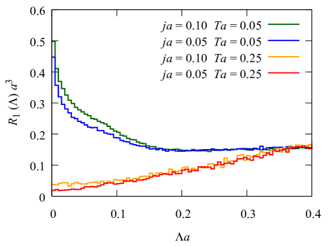
Figure 3: Spectral density $R_{1}(\Lambda)$ in the lattice simulation for $N=2$ and $g/a^{2}=1$. The averages over 500 configurations are shown.

We also checked the correspondence to RMT in a small finite volume $V/a^{3}=4^{3}$. To increase the number of configurations, we adopted the quenched approximation, which is frequently used in lattice QCD to reduce the computational cost Rothe (1992). In the quenched approximation, the fermion determinant in the measure (8) is neglected. The measure is thus given by a product of independent Gaussian weights for $\phi(x)$, which helps to speed up the simulation extremely. Since quenched configurations are independent of $j$, singular-value distributions have no dependence on $j$. In Fig. 4, the microscopic spectral density $\rho(\lambda)$ and the smallest singular-value distribution $P(\lambda_{\rm min})$ are shown. In the quenched chGOE with trivial topology ($\nu=0$), they are analytically given by Verbaarschot (1994b); Forrester et al. (1999)

$$\begin{split}\rho_{\scriptscriptstyle\text{RMT}}(\lambda)=&\frac{\lambda}{2}\{J_{0}(\lambda)^{2}+J_{1}(\lambda)^{2}\}\\ &+\frac{1}{2}J_{0}(\lambda)\bigg{(}1-\int_{0}^{\lambda}\!\!\!\mathrm{d}x~{}J_{0}(x)\bigg{)}\end{split}$$ (46)

and Forrester (1993)

$$P_{\scriptscriptstyle\text{RMT}}(\lambda_{\rm min}) =\frac{2+\lambda_{\rm min}}{4}\exp\left(-\frac{\lambda_{\rm min}^{2}}{8}-\frac{\lambda_{\rm min}}{2}\right),$$ (47)

respectively, which are drawn in Fig. 4 for comparison. Although these analytical solutions of RMT are parameter free if $\Phi$ is known, here $\Phi$ is treated as a fitting parameter. At a low temperature ($Ta=0.05$), the lattice simulation nicely reproduces the predictions of RMT. At a high temperature ($Ta=0.25$), the lattice simulation deviates from RMT and approaches the Poisson distribution

$$P(\lambda_{\rm min})=\exp(-\lambda_{\rm min})\,,$$ (48)

which signals absence of a level correlation.

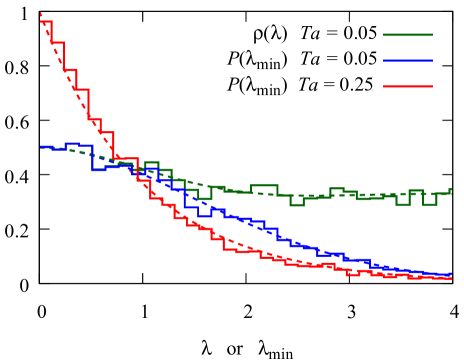
Figure 4: Microscopic spectral density $\rho(\lambda)$ and the smallest singular-value distribution $P(\lambda_{\rm min})$ in the quenched lattice simulation with $g/a^{2}=3$. The green, blue, and red broken curves are the predictions (46) and (47) by RMT and the Poisson statistics (48), respectively. The averages over 5000 configurations are shown.

VII Summary and perspective

In this work, we studied multi-component fermionic superfluids and derived a number of rigorous results by using theoretical methods that hardly appear in conventional studies of nonrelativistic systems but are well established in the field of Quantum Chromodynamics (QCD). By relating the order parameters of spontaneous symmetry breaking to the singular-value spectrum of a single operator $W$ [Eq. (7)] we derived a nonrelativistic analog of the Banks–Casher relation in QCD, which enables us to extract the bifermion condensate $\left\langle\psi\psi\right\rangle$ from the spectrum reliably. Furthermore we have shown, through a spectral analysis of $W$, that $\text{U}(1)$ and $\text{SU}(N)$ symmetry of the $N$-component Fermi gas must be restored/broken simultaneously. This imposes a strong constraint on the phase diagram by precluding intermediate phases where either $\text{U}(1)$ or $\text{SU}(N)$ is broken and the other is not.

We also developed a low-energy effective theory of Nambu–Goldstone modes in the superfluid phase for general even $N$, and rigorously derived a formula which expresses the slope of the spectral density near zero in terms of low-energy constants that enter the effective Lagrangian. This is an analog of the Smilga–Stern relation in QCD. In addition, we pointed out that the effective theory can be mapped to a random matrix theory in the $\varepsilon$-regime. From this correspondence we found an analytical formula for the spectral density near zero. This provides us with a novel, numerically clean method to extract the bifermion condensate through fitting to the numerical data of the spectrum. We confirmed these analytical calculations by the path-integral Monte Carlo simulations.

It should be emphasized that the analysis in this paper involves no uncontrolled approximations and is valid under quite general conditions for temperature, density and the interaction strength, as long as the path-integral measure is positive definite. Our results can be used to benchmark other theoretical methods.

There are various future directions. The multi-component Hubbard model can be studied in the same manner. This may add to our knowledge of the rigorous results of the Hubbard model. It is also worthwhile to extend the present work to other cases of $N$; in particular, the symmetry analysis based on the multi-point correlation functions in Sec. III to $N\geq 6$, the Smilga–Stern-like relation in Sec. IV to $N=2$, and the numerical checks of correspondence to RMT in Sec. VI to unquenched $N\geq 2$. The extension of our framework to theories with odd $N$ or repulsive interactions is a more challenging problem.

Appendix A Spectral density in a free theory

In the free limit $g\to 0$, the spectral density can be obtained analytically. The spectral density is independent of $j$ in a free theory. At $T=0$,

$$\quad R_{1}(\Lambda)$$

$$=\frac{1}{\beta V}\bigg{\langle}\sum_{n}\delta(\Lambda_{n}-\Lambda)\bigg{\rangle}$$

$$=\frac{2\Lambda}{\beta V}\operatorname{tr}\left[\delta(WW^{\dagger}-\Lambda^{2})\right]$$

$$=\frac{2\Lambda}{\beta V}\operatorname{tr}\left[\delta\bigg{(}-\partial_{\tau}^{2}+\left(-\frac{\nabla^{2}}{2m}-\mu\right)^{2}-\Lambda^{2}\bigg{)}\right]$$

$$=2(2m)^{D/2}\Lambda\!\int\!\frac{\mathrm{d}\omega}{2\pi}\!\int\!\!\frac{\mathrm{d}^{D}q}{(2\pi)^{D}}~{}\delta\left(\omega^{2}+(q^{2}-\mu)^{2}-\Lambda^{2}\right)$$

$$=\frac{C_{D}}{(2\pi)^{D}}(2m)^{D/2}\Lambda~{}\times$$

$$\qquad\times\int\!\frac{\mathrm{d}\omega}{2\pi}\!\int_{0}^{\infty}\!\!\!\mathrm{d}r~{}r^{(D-2)/2}~{}\delta\left(\omega^{2}+(r-\mu)^{2}-\Lambda^{2}\right)$$

$$=\frac{C_{D}}{(2\pi)^{D+1}}(2m)^{D/2}\Lambda~{}\times$$

$$\qquad\times\int_{0}^{\infty}\!\!\!\mathrm{d}r~{}r^{(D-2)/2}~{}\frac{\Theta\big{(}\Lambda^{2}-\left(r-\mu\right)^{2}\big{)}}{\sqrt{\Lambda^{2}-\left(r-\mu\right)^{2}}}\,,$$ (49)

where $\Theta(x)$ is a step function and $C_{1}=2$, $C_{2}=2\pi$ and $C_{3}=4\pi$. The integrand of (49) is nonzero for $(r-\mu)^{2}\leq\Lambda^{2}$, i.e., $\mu-\Lambda\leq r\leq\mu+\Lambda$. We divide the $(\mu,\Lambda)$-plane into two regions: $\mu\geq\Lambda$ and $\Lambda\geq\mu$.
$\bullet$ Case I: $\mu\geq\Lambda$
Writing $r=\mu+\Lambda\cos\theta$ ($0\leq\theta\leq\pi$), we obtain

$$\quad R_{1}(\Lambda)$$

$$=\frac{C_{D}}{(2\pi)^{D+1}}(2m)^{D/2}\Lambda\!\int_{\mu-\Lambda}^{\mu+\Lambda}\!\!\!\mathrm{d}r\frac{r^{(D-2)/2}}{\sqrt{\Lambda^{2}-\left(r-\mu\right)^{2}}}$$

$$=\frac{C_{D}}{(2\pi)^{D+1}}(2m)^{D/2}\Lambda\!\int_{0}^{\pi}\!\!\mathrm{d}\theta\left(\mu+\Lambda\cos\theta\right)^{(D-2)/2}$$

$$=\left\{\begin{array}[]{ll}\displaystyle\frac{m}{2\pi}\Lambda&[D=2]\vspace{3pt}\\ \displaystyle\frac{(2m)^{3/2}}{2\pi^{3}}\Lambda\sqrt{\mu+\Lambda}\operatorname*{\mathbf{E}}\left(\frac{2\Lambda}{\mu+\Lambda}\right)&[D=3]\end{array}\right.,$$ (52)

where $\operatorname*{\mathbf{E}}(x)\equiv\int_{0}^{\pi/2}\mathrm{d}\theta\sqrt{1-x\sin^{2}\theta}$ is the complete elliptic integral of the second kind. Interestingly, $R_{1}(\Lambda)$ has no $\mu$-dependence for $D=2$.
$\bullet$ Case II: $\Lambda\geq\mu$

$$\quad R_{1}(\Lambda)$$

$$=\frac{C_{D}}{(2\pi)^{D+1}}(2m)^{D/2}\Lambda\!\int_{0}^{\mu+\Lambda}\!\!\!\mathrm{d}r\frac{r^{(D-2)/2}}{\sqrt{\Lambda^{2}-\left(r-\mu\right)^{2}}}$$

$$=\frac{C_{D}}{(2\pi)^{D+1}}(2m)^{D/2}\Lambda~{}\times$$

$$\qquad\times\int_{0}^{\Xi}\!\!\mathrm{d}\theta\left(\mu+\Lambda\cos\theta\right)^{(D-2)/2}\Big{|}_{\Xi:=\cos^{-1}(-\frac{\mu}{\Lambda})}$$

$$=\left\{\begin{array}[]{ll}\displaystyle\frac{m}{2\pi^{2}}\Xi\Lambda&[D=2]\vspace{3pt}\\ \displaystyle\frac{(2m)^{3/2}}{2\pi^{3}}\Lambda\sqrt{\mu+\Lambda}\operatorname*{\mathbf{E}}\left(\frac{\Xi}{2}\bigg{|}\frac{2\Lambda}{\mu+\Lambda}\right)&[D=3]\end{array}\right.,$$ (55)

where $\operatorname*{\mathbf{E}}(\varphi|x)\equiv\int_{0}^{\varphi}\mathrm{d}\theta\sqrt{1-x\sin^{2}\theta}$ is the incomplete elliptic integral of the second kind. If we formally set $\Xi=\pi$, (55) reduces to (52).

Figure 5 displays $R_{1}(\Lambda)$.

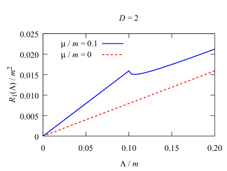
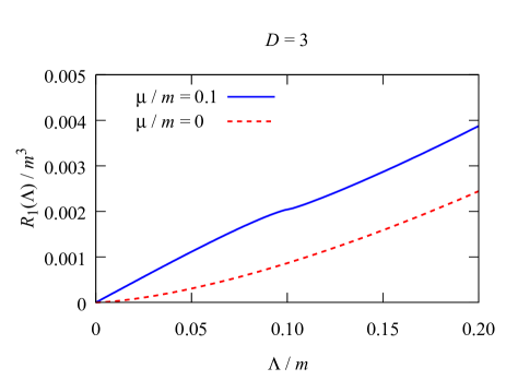
Figure 5: Spectral density in the non-interacting limit at $T=0$ in $2$ (top) and $3$ (bottom) spatial dimensions.

In the limit $\mu\to 0$ (or $\Lambda\gg\mu$), one finds from (55)

$$R_{1}(\Lambda)\sim\left\{\begin{array}[]{ll}\displaystyle\frac{m}{4\pi}\Lambda&~{}[D=2]\vspace{3pt}\\ \displaystyle c\frac{(2m)^{3/2}}{2\pi^{3}}\Lambda\sqrt{\Lambda}&~{}[D=3]\end{array}\right.,\$$ (58)

where $\displaystyle c\equiv\operatorname*{\mathbf{E}}\left(\frac{\pi}{4}\bigg{|}2\right)=0.59907\dots$ is a numerical constant. In contrast, for $\Lambda\ll\mu$, (52) becomes

$$R_{1}(\Lambda)\sim\left\{\begin{array}[]{ll}\displaystyle\frac{m}{2\pi}\Lambda&~{}[D=2]\vspace{3pt}\\ \displaystyle\frac{\pi}{2}\frac{(2m)^{3/2}}{2\pi^{3}}\sqrt{\mu}\,\Lambda&~{}[D=3]\end{array}\right..$$ (61)

At $T>0$, the continuous frequency $\omega$ should be replaced with the Matsubara frequency $\omega_{n}=(2n+1)\pi T$. This means, in a plane basis,

$$WW^{\dagger}=\omega_{n}^{2}+\left(\frac{\bm{p}^{2}}{2m}-\mu\right)^{2}\geq\omega_{0}^{2}=(\pi T)^{2}\,.$$ (62)

Therefore $R_{1}(\Lambda)$ vanishes identically on the interval $\Lambda\in[0,\pi T]$.

Appendix B Correlation functions

In this appendix, we summarize technical formulas of the correlation functions used in Sec. III. The propagators for the theory (8) read

$$\mathchoice{\vbox{\hbox to0.0pt{\kern 0.0pt\kern 3.25696pt\hbox{\vrule width=0.50003pt,height=0.0pt,depth=4.30554pt\vrule width=20.00699pt,height=0.0pt,depth=0.50003pt\vrule width=0.50003pt,height=0.0pt,depth=4.30554pt}\hss}\vskip 2.15277pt\vskip 6.94444pt}}{\vbox{\hbox to0.0pt{\kern 0.0pt\kern 3.25696pt\hbox{\vrule width=0.50003pt,height=0.0pt,depth=4.30554pt\vrule width=20.00699pt,height=0.0pt,depth=0.50003pt\vrule width=0.50003pt,height=0.0pt,depth=4.30554pt}\hss}\vskip 2.15277pt\vskip 6.94444pt}}{\vbox{\hbox to0.0pt{\kern 0.0pt\kern 2.27986pt\hbox{\vrule width=0.50003pt,height=0.0pt,depth=4.30554pt\vrule width=14.00488pt,height=0.0pt,depth=0.50003pt\vrule width=0.50003pt,height=0.0pt,depth=4.30554pt}\hss}\vskip 2.15277pt\vskip 4.8611pt}}{\vbox{\hbox to0.0pt{\kern 0.0pt\kern 1.62848pt\hbox{\vrule width=0.50003pt,height=0.0pt,depth=4.30554pt\vrule width=10.00348pt,height=0.0pt,depth=0.50003pt\vrule width=0.50003pt,height=0.0pt,depth=4.30554pt}\hss}\vskip 2.15277pt\vskip 3.47221pt}}\psi(x)\psi^{\dagger}(y) =\langle x|\frac{\mathbb{1}_{N}}{W^{\dagger}W+j^{2}}W^{\dagger}|y\rangle$$ (63a)

$$\mathchoice{\vbox{\hbox to0.0pt{\kern 0.0pt\kern 3.25696pt\hbox{\vrule width=0.50003pt,height=0.0pt,depth=4.30554pt\vrule width=20.00699pt,height=0.0pt,depth=0.50003pt\vrule width=0.50003pt,height=0.0pt,depth=4.30554pt}\hss}\vskip 2.15277pt\vskip 6.94444pt}}{\vbox{\hbox to0.0pt{\kern 0.0pt\kern 3.25696pt\hbox{\vrule width=0.50003pt,height=0.0pt,depth=4.30554pt\vrule width=20.00699pt,height=0.0pt,depth=0.50003pt\vrule width=0.50003pt,height=0.0pt,depth=4.30554pt}\hss}\vskip 2.15277pt\vskip 6.94444pt}}{\vbox{\hbox to0.0pt{\kern 0.0pt\kern 2.27986pt\hbox{\vrule width=0.50003pt,height=0.0pt,depth=4.30554pt\vrule width=14.00488pt,height=0.0pt,depth=0.50003pt\vrule width=0.50003pt,height=0.0pt,depth=4.30554pt}\hss}\vskip 2.15277pt\vskip 4.8611pt}}{\vbox{\hbox to0.0pt{\kern 0.0pt\kern 1.62848pt\hbox{\vrule width=0.50003pt,height=0.0pt,depth=4.30554pt\vrule width=10.00348pt,height=0.0pt,depth=0.50003pt\vrule width=0.50003pt,height=0.0pt,depth=4.30554pt}\hss}\vskip 2.15277pt\vskip 3.47221pt}}\psi(x)\psi^{T}(y) =\langle x|\frac{jI}{W^{\dagger}W+j^{2}}|y\rangle$$ (63b)

$$\mathchoice{\vbox{\hbox to0.0pt{\kern 0.0pt\kern 3.25696pt\hbox{\vrule width=0.50003pt,height=0.0pt,depth=4.30554pt\vrule width=22.80699pt,height=0.0pt,depth=0.50003pt\vrule width=0.50003pt,height=0.0pt,depth=4.30554pt}\hss}\vskip 2.15277pt\vskip 6.94444pt}}{\vbox{\hbox to0.0pt{\kern 0.0pt\kern 3.25696pt\hbox{\vrule width=0.50003pt,height=0.0pt,depth=4.30554pt\vrule width=22.80699pt,height=0.0pt,depth=0.50003pt\vrule width=0.50003pt,height=0.0pt,depth=4.30554pt}\hss}\vskip 2.15277pt\vskip 6.94444pt}}{\vbox{\hbox to0.0pt{\kern 0.0pt\kern 2.27986pt\hbox{\vrule width=0.50003pt,height=0.0pt,depth=4.30554pt\vrule width=16.00488pt,height=0.0pt,depth=0.50003pt\vrule width=0.50003pt,height=0.0pt,depth=4.30554pt}\hss}\vskip 2.15277pt\vskip 4.8611pt}}{\vbox{\hbox to0.0pt{\kern 0.0pt\kern 1.62848pt\hbox{\vrule width=0.50003pt,height=0.0pt,depth=4.30554pt\vrule width=12.00348pt,height=0.0pt,depth=0.50003pt\vrule width=0.50003pt,height=0.0pt,depth=4.30554pt}\hss}\vskip 2.15277pt\vskip 3.47221pt}}\psi^{*}(x)\psi^{T}(y) =\langle x|-\frac{\mathbb{1}_{N}}{WW^{\dagger}+j^{2}}W|y\rangle$$ (63c)

$$\mathchoice{\vbox{\hbox to0.0pt{\kern 0.0pt\kern 3.25696pt\hbox{\vrule width=0.50003pt,height=0.0pt,depth=4.30554pt\vrule width=22.80699pt,height=0.0pt,depth=0.50003pt\vrule width=0.50003pt,height=0.0pt,depth=4.30554pt}\hss}\vskip 2.15277pt\vskip 6.94444pt}}{\vbox{\hbox to0.0pt{\kern 0.0pt\kern 3.25696pt\hbox{\vrule width=0.50003pt,height=0.0pt,depth=4.30554pt\vrule width=22.80699pt,height=0.0pt,depth=0.50003pt\vrule width=0.50003pt,height=0.0pt,depth=4.30554pt}\hss}\vskip 2.15277pt\vskip 6.94444pt}}{\vbox{\hbox to0.0pt{\kern 0.0pt\kern 2.27986pt\hbox{\vrule width=0.50003pt,height=0.0pt,depth=4.30554pt\vrule width=16.00488pt,height=0.0pt,depth=0.50003pt\vrule width=0.50003pt,height=0.0pt,depth=4.30554pt}\hss}\vskip 2.15277pt\vskip 4.8611pt}}{\vbox{\hbox to0.0pt{\kern 0.0pt\kern 1.62848pt\hbox{\vrule width=0.50003pt,height=0.0pt,depth=4.30554pt\vrule width=12.00348pt,height=0.0pt,depth=0.50003pt\vrule width=0.50003pt,height=0.0pt,depth=4.30554pt}\hss}\vskip 2.15277pt\vskip 3.47221pt}}\psi^{*}(x)\psi^{\dagger}(y) =\langle x|-\frac{jI}{WW^{\dagger}+j^{2}}|y\rangle.$$ (63d)

It is a straightforward exercise to evaluate the integrated connected correlator (15) for the multiplet $(\Pi^{0},\Delta^{0},\Pi^{A},\Delta^{A})$ defined in Eq. (14). Noting that the disconnected piece is nonzero only for $\Delta^{0}$, we find

$$\mathsf{C}_{\Pi^{0}} =2\bigg{\langle}\!\operatorname{tr}\frac{1}{W^{\dagger}W+j^{2}}\bigg{\rangle},$$ (64a)

$$\mathsf{C}_{\Delta^{0}} =2\bigg{\langle}\!\operatorname{tr}\frac{W^{\dagger}W-j^{2}}{(W^{\dagger}W+j^{2})^{2}}\bigg{\rangle}+2N\bigg{\langle}\!\bigg{(}\!\operatorname{tr}\frac{j}{W^{\dagger}W+j^{2}}\bigg{)}^{2}\bigg{\rangle}$$

$$\quad-2N\bigg{\langle}\!\operatorname{tr}\frac{j}{W^{\dagger}W+j^{2}}\bigg{\rangle}^{2},$$ (64b)

$$\mathsf{C}_{\Pi^{A}} =4\operatorname{tr}(T^{A}T^{A})\bigg{\langle}\!\operatorname{tr}\frac{1}{W^{\dagger}W+j^{2}}\bigg{\rangle},$$ (64c)

$$\mathsf{C}_{\Delta^{A}} =4\operatorname{tr}(T^{A}T^{A})\bigg{\langle}\!\operatorname{tr}\frac{W^{\dagger}W-j^{2}}{(W^{\dagger}W+j^{2})^{2}}\bigg{\rangle}.$$ (64d)

In deriving these results we used the identity

$$\operatorname{tr}\frac{j}{WW^{\dagger}+j^{2}}=\operatorname{tr}\frac{j}{W^{\dagger}W+j^{2}}\,.$$ (65)

Note that an analogue of this relation for the Dirac operator does not hold in QCD because of the index theorem. The summation over $A$ can be easily taken with the help of the identity

$$\sum_{A}T^{A}T^{A} =\frac{N^{2}-N-2}{4N}\mathbb{1}_{N}\,.$$ (66)

Appendix C Derivation of $\chi_{AB}(j)$

Here, we derive Eqs. (32), (33), and (34). In the microscopic theory, the partition function (8) is modified by the generalized source term (24) as $Z(j)\to Z(J)$. The susceptibility is

$$\begin{split}\chi_{AB}(j)&\equiv\lim_{\forall j_{A}\to 0}\lim_{V\to\infty}\frac{1}{\beta V}\frac{\partial^{2}}{\partial j_{A}\partial j_{B}}\log Z(J)\\ &=\lim_{\forall j_{A}\to 0}\lim_{V\to\infty}\frac{1}{4\beta V}\int_{x}\int_{y}\left\langle\Delta^{A}(x)\Delta^{B}(y)\right\rangle_{J}\\ &=\frac{\delta_{AB}}{2}\int_{0}^{\infty}\!\!\!\mathrm{d}\Lambda\,\frac{\Lambda^{2}-j^{2}}{(\Lambda^{2}+j^{2})^{2}}R_{1}(\Lambda)\,.\end{split}$$ (67)

This gives Eq. (32). While the average $\left\langle\cdots\right\rangle_{J}$ is taken over the measure with a generalized source term (24), $R_{1}(\Lambda)$ is given by the original measure (8) in the $j_{A}\to 0$ limit.

In EFT, we assume $T=0$ for the sake of simplicity. The $j_{A}$-dependent part of the source term is

$$\mathrm{Re}\operatorname{tr}(J\tilde{\Sigma}) =j_{A}\mathcal{V}^{A}+\dots$$ (68)

with

$$\mathcal{V}^{A} \equiv\frac{1}{4F^{2}}\operatorname{tr}\!\left(T^{A}\{T^{P},T^{Q}\}\right)\pi^{P}\pi^{Q}+\frac{1}{2Ff}\phi\pi^{A}$$ (69)

in the leading order of $\phi$ and $\pi^{A}$. Hence

$$\chi_{AB}(j)=\frac{\Phi^{2}}{\beta V}\int_{x}\int_{y}\left\langle\mathcal{V}^{A}(x)\mathcal{V}^{B}(y)\right\rangle_{\text{1-loop}}$$ (70)

where $\left\langle\mathcal{V}^{A}\right\rangle=0$ was used. The subscript implies we will perform a one-loop analysis, which is sufficient to see the leading infrared behavior. As the cross term $\left\langle\pi^{P}\pi^{Q}\phi\pi^{A}\right\rangle=0$, we get

$$\begin{split}&\chi_{AB}(j)\\ &=\frac{\Phi^{2}}{8F^{4}}\operatorname{tr}\!\left(T^{A}\{T^{P},T^{Q}\}\right)\operatorname{tr}\!\left(T^{B}\{T^{P},T^{Q}\}\right)\times\\ &\qquad\quad\times\int_{p}\frac{1}{(\omega^{2}+v^{2}\bm{p}^{2}+m_{\pi}^{2})^{2}}\\ &\quad+\delta_{AB}\frac{\Phi^{2}}{4F^{2}f^{2}}\int_{p}\frac{1}{\omega^{2}+v^{2}\bm{p}^{2}+m_{\pi}^{2}}\frac{1}{\omega^{2}+\tilde{v}^{2}\bm{p}^{2}+m_{\phi}^{2}}\,,\end{split}$$ (71)

with $\int_{p}\equiv\int\frac{\mathrm{d}\omega}{2\pi}\int\frac{\mathrm{d}^{D}p}{(2\pi)^{D}}$ . We consult Toublan and Verbaarschot (1999) to obtain

$$\operatorname{tr}\!\left(T^{A}\{T^{P},T^{Q}\}\right)\operatorname{tr}\!\left(T^{B}\{T^{P},T^{Q}\}\right)$$

$$\qquad=\frac{(N-4)(N+2)}{8N}\delta_{AB}\,.$$ (72)

The momentum integrals in Eq. (71) are divergent in the limit $j\to 0$ for $D\leq 3$. At $D=3$, the leading singularity in $j\to 0$ is

$$\int_{p}\frac{1}{(\omega^{2}+v^{2}\bm{p}^{2}+m_{\pi}^{2})^{2}}\simeq-\frac{1}{16\pi^{2}}\frac{1}{v^{3}}\log j\,,$$ (73)

$$\int_{p}\frac{1}{\omega^{2}+v^{2}\bm{p}^{2}+m_{\pi}^{2}}\frac{1}{\omega^{2}+\tilde{v}^{2}\bm{p}^{2}+m_{\phi}^{2}}$$

$$\qquad\simeq-\frac{1}{8\pi^{2}}\frac{1}{v\tilde{v}(v+\tilde{v})}\log j\,.$$ (74)

We used $m_{\pi}^{2}=j\Phi/2F^{2}$ and $m_{\phi}^{2}=jN\Phi/f^{2}$. Collecting everything, we obtain Eqs. (33) and (34). In the same way one can show $\chi_{AB}(j)\sim 1/\sqrt{j}$ at $D=2$.

References

- Kapitza (1938) P. Kapitza, Nature 141, 74 (1938).
- Osheroff et al. (1972) D. D. Osheroff, R. C. Richardson, and D. M. Lee, Phys. Rev. Lett. 28, 885 (1972).
- Anderson et al. (1995) M. H. Anderson, J. R. Ensher, M. R. Matthews, C. E. Wieman, and E. A. Cornell, Science 269, 198 (1995).
- Davis et al. (1995) K. B. Davis, M. O. Mewes, M. R. Andrews, N. J. van Druten, D. S. Durfee, D. M. Kurn, and W. Ketterle, Phys. Rev. Lett. 75, 3969 (1995).
- Bardeen et al. (1957) J. Bardeen, L. N. Cooper, and J. R. Schrieffer, Phys. Rev. 108, 1175 (1957).
- Nambu (1960) Y. Nambu, Phys. Rev. 117, 648 (1960).
- Nambu and Jona-Lasinio (1961a) Y. Nambu and G. Jona-Lasinio, Phys. Rev. 122, 345 (1961a).
- Nambu and Jona-Lasinio (1961b) Y. Nambu and G. Jona-Lasinio, Phys. Rev. 124, 246 (1961b).
- Higgs (1964a) P. W. Higgs, Phys. Lett. 12, 132 (1964a).
- Englert and Brout (1964) F. Englert and R. Brout, Phys. Rev. Lett. 13, 321 (1964).
- Higgs (1964b) P. W. Higgs, Phys. Rev. Lett. 13, 508 (1964b).
- Gaponov et al. (1996) Y. V. Gaponov, D. Vladimirov, and J. Bang, Acta Physica Hungarica New Series Heavy Ion Physics 3, 189 (1996).
- Taie et al. (2010) S. Taie, Y. Takasu, S. Sugawa, R. Yamazaki, T. Tsujimoto, R. Murakami, and Y. Takahashi, Physical Review Letters 105, 190401 (2010), arXiv:1005.3670 [cond-mat.quant-gas] .
- Honerkamp and Hofstetter (2004a) C. Honerkamp and W. Hofstetter, Physical Review Letters 92, 170403 (2004a), cond-mat/0309374 .
- Taie et al. (2012) S. Taie, R. Yamazaki, S. Sugawa, and Y. Takahashi, Nature Physics 8, 825 (2012), arXiv:1208.4883 [cond-mat.quant-gas] .
- Wu et al. (2003) C. Wu, J.-p. Hu, and S.-c. Zhang, Phys. Rev. Lett. 91, 186402 (2003), arXiv:cond-mat/0302165 [cond-mat.str-el] .
- Honerkamp and Hofstetter (2004b) C. Honerkamp and W. Hofstetter, Phys. Rev. B70, 094521 (2004b), cond-mat/0403166 .
- Veillette et al. (2007) M. Y. Veillette, D. E. Sheehy, and L. Radzihovsky, Phys. Rev. A75, 043614 (2007), arXiv:cond-mat/0610798 [cond-mat.other] .
- Cherng et al. (2007) R. W. Cherng, G. Refael, and E. Demler, Phys. Rev. Lett. 99,, 130406 (2007), 0705.0347 .
- Gorshkov et al. (2009) A. V. Gorshkov, M. Hermele, V. Gurarie, C. Xu, P. S. Julienne, J. Ye, P. Zoller, E. Demler, M. D. Lukin, and A. M. Rey, Nature Phys. 6,, 289 (2009), 0905.2610 .
- Cazalilla et al. (2009) M. A. Cazalilla, A. F. Ho, and M. Ueda, New Journal of Physics 11,, 103033 (2009), 0905.4948 .
- Szirmai and Lewenstein (2010) E. Szirmai and M. Lewenstein, Europhysics Letters 93,, 66005 (2010), 1009.4868 .
- Yip (2011) S. K. Yip, Phys. Rev. A83, 063607 (2011), 1101.1714 .
- hsuan Hung et al. (2011) H. hsuan Hung, Y. Wang, and C. Wu, Phys. Rev. B 84,, 054406 (2011), 1103.1926 .
- Yip et al. (2014) S. K. Yip, B.-L. Huang, and J.-S. Kao, Phys. Rev. A89, 043610 (2014), 1312.6765 .
- Zhang et al. (2014) X. Zhang, M. Bishof, S. L. Bromley, C. V. Kraus, M. S. Safronova, P. Zoller, A. M. Rey, and J. Ye, Science 345, 1467 (2014), arXiv:1403.2964 [cond-mat.quant-gas] .
- Cazalilla and Rey (2014) M. Cazalilla and A. Rey, Rept. Prog. Phys. 77, 124401 (2014), arXiv:1403.2792 [cond-mat.quant-gas] .
- Banks and Casher (1980) T. Banks and A. Casher, Nucl. Phys. B169, 103 (1980).
- Akemann et al. (2005) G. Akemann, J. C. Osborn, K. Splittorff, and J. J. M. Verbaarschot, Nucl. Phys. B712, 287 (2005), arXiv:hep-th/0411030 [hep-th] .
- Osborn et al. (2005) J. C. Osborn, K. Splittorff, and J. J. M. Verbaarschot, Phys. Rev. Lett. 94, 202001 (2005), arXiv:hep-th/0501210 [hep-th] .
- Kanazawa et al. (2011) T. Kanazawa, T. Wettig, and N. Yamamoto, JHEP 12, 007 (2011), arXiv:1110.5858 [hep-ph] .
- Kanazawa and Wettig (2014) T. Kanazawa and T. Wettig, JHEP 10, 55 (2014), arXiv:1406.6131 [hep-ph] .
- Verbaarschot and Wettig (2014) J. J. M. Verbaarschot and T. Wettig, Phys. Rev. D90, 116004 (2014), arXiv:1407.8393 [hep-th] .
- Shushpanov and Smilga (1997) I. A. Shushpanov and A. V. Smilga, Phys. Lett. B402, 351 (1997), arXiv:hep-ph/9703201 [hep-ph] .
- Peskin (1980) M. E. Peskin, Nucl. Phys. B175, 197 (1980).
- Kogut et al. (2000) J. B. Kogut, M. A. Stephanov, D. Toublan, J. J. M. Verbaarschot, and A. Zhitnitsky, Nucl. Phys. B582, 477 (2000), arXiv:hep-ph/0001171 [hep-ph] .
- Vafa and Witten (1984) C. Vafa and E. Witten, Nucl. Phys. B234, 173 (1984).
- Kosower (1984) D. A. Kosower, Phys. Lett. B144, 215 (1984).
- Rajagopal and Wilczek (2000) K. Rajagopal and F. Wilczek, (2000), arXiv:hep-ph/0011333 [hep-ph] .
- Alford et al. (2008) M. G. Alford, A. Schmitt, K. Rajagopal, and T. Schäfer, Rev. Mod. Phys. 80, 1455 (2008), arXiv:0709.4635 [hep-ph] .
- Stern (1998) J. Stern, (1998), arXiv:hep-ph/9801282 .
- Kogan et al. (1999) I. I. Kogan, A. Kovner, and M. A. Shifman, Phys. Rev. D59, 016001 (1999), arXiv:hep-ph/9807286 .
- Kanazawa (2015) T. Kanazawa, JHEP 10, 010 (2015), arXiv:1507.06376 [hep-ph] .
- Shuryak (1994) E. V. Shuryak, Comments Nucl.Part.Phys. 21, 235 (1994), arXiv:hep-ph/9310253 [hep-ph] .
- Cohen (1996) T. D. Cohen, Phys.Rev. D54, 1867 (1996), arXiv:hep-ph/9601216 [hep-ph] .
- Bernard et al. (1997) C. W. Bernard, T. Blum, C. E. Detar, S. A. Gottlieb, U. M. Heller, J. E. Hetrick, K. Rummukainen, R. Sugar, D. Toussaint, and M. Wingate, Phys. Rev. Lett. 78, 598 (1997), arXiv:hep-lat/9611031 [hep-lat] .
- Chandrasekharan et al. (1999) S. Chandrasekharan, D. Chen, N. H. Christ, W.-J. Lee, R. Mawhinney, and P. M. Vranas, Phys. Rev. Lett. 82, 2463 (1999), arXiv:hep-lat/9807018 [hep-lat] .
- Edwards et al. (2000) R. G. Edwards, U. M. Heller, J. E. Kiskis, and R. Narayanan, Phys. Rev. D61, 074504 (2000), arXiv:hep-lat/9910041 [hep-lat] .
- Kanazawa and Yamamoto (2015) T. Kanazawa and N. Yamamoto, (2015), arXiv:1508.02416 [hep-th] .
- Hidaka et al. (2015) Y. Hidaka, K. Kamikado, T. Kanazawa, and T. Noumi, Phys. Rev. D92, 034003 (2015), arXiv:1505.00848 [hep-ph] .
- Radzihovsky (2011) L. Radzihovsky, Phys. Rev. A 84, 023611 (2011), arXiv:1102.4903 [cond-mat] .
- Radzihovsky (2012) L. Radzihovsky, Physica C: Superconductivity 481, 189 (2012), arXiv:1112.0773 [cond-mat] .
- Gusynin et al. (1994) V. P. Gusynin, V. A. Miransky, and I. A. Shovkovy, Phys. Rev. Lett. 73, 3499 (1994), [Erratum: Phys. Rev. Lett.76,1005(1996)], arXiv:hep-ph/9405262 [hep-ph] .
- Gusynin et al. (1995) V. P. Gusynin, V. A. Miransky, and I. A. Shovkovy, Phys. Rev. D52, 4718 (1995), arXiv:hep-th/9407168 [hep-th] .
- Das and Hott (1996) A. K. Das and M. B. Hott, Phys. Rev. D53, 2252 (1996), arXiv:hep-th/9504086 [hep-th] .
- Fisher et al. (1973) M. E. Fisher, M. N. Barber, and D. Jasnow, Phys. Rev. A8, 1111 (1973).
- Hasenfratz and Leutwyler (1990) P. Hasenfratz and H. Leutwyler, Nucl. Phys. B343, 241 (1990).
- Smilga and Stern (1993) A. V. Smilga and J. Stern, Phys. Lett. B318, 531 (1993).
- Osborn et al. (1999) J. C. Osborn, D. Toublan, and J. J. M. Verbaarschot, Nucl. Phys. B540, 317 (1999), arXiv:hep-th/9806110 .
- Toublan and Verbaarschot (1999) D. Toublan and J. J. M. Verbaarschot, Nucl. Phys. B560, 259 (1999), arXiv:hep-th/9904199 .
- Leutwyler (1994) H. Leutwyler, Phys. Rev. D49, 3033 (1994), arXiv:hep-ph/9311264 [hep-ph] .
- Watanabe and Murayama (2012) H. Watanabe and H. Murayama, Phys. Rev. Lett. 108, 251602 (2012), arXiv:1203.0609 [hep-th] .
- Hidaka (2013) Y. Hidaka, Phys. Rev. Lett. 110, 091601 (2013), arXiv:1203.1494 [hep-th] .
- Takahashi and Nitta (2015) D. A. Takahashi and M. Nitta, Annals Phys. 354, 101 (2015), arXiv:1404.7696 [cond-mat.quant-gas] .
- Watanabe and Murayama (2014) H. Watanabe and H. Murayama, Phys. Rev. X4, 031057 (2014), arXiv:1402.7066 [hep-th] .
- Andersen et al. (2014) J. O. Andersen, T. Brauner, C. P. Hofmann, and A. Vuorinen, JHEP 08, 088 (2014), arXiv:1406.3439 [hep-ph] .
- Smilga and Verbaarschot (1995) A. V. Smilga and J. J. M. Verbaarschot, Phys. Rev. D51, 829 (1995), arXiv:hep-th/9404031 .
- Kogut et al. (1999) J. B. Kogut, M. A. Stephanov, and D. Toublan, Phys. Lett. B464, 183 (1999), arXiv:hep-ph/9906346 [hep-ph] .
- Kanazawa et al. (2009) T. Kanazawa, T. Wettig, and N. Yamamoto, JHEP 08, 003 (2009), arXiv:0906.3579 [hep-ph] .
- He et al. (2006) L. He, M. Jin, and P. Zhuang, Phys. Rev. A74, 033604 (2006), arXiv:cond-mat/0604580 [cond-mat] .
- Schafer et al. (2001) T. Schafer, D. T. Son, M. A. Stephanov, D. Toublan, and J. J. M. Verbaarschot, Phys. Lett. B522, 67 (2001), arXiv:hep-ph/0108210 [hep-ph] .
- Duan et al. (2001) Z.-y. Duan, P. S. Rodrigues da Silva, and F. Sannino, Nucl. Phys. B592, 371 (2001), arXiv:hep-ph/0001303 [hep-ph] .
- Lenaghan et al. (2002) J. T. Lenaghan, F. Sannino, and K. Splittorff, Phys. Rev. D65, 054002 (2002), arXiv:hep-ph/0107099 [hep-ph] .
- Splittorff et al. (2001) K. Splittorff, D. T. Son, and M. A. Stephanov, Phys. Rev. D64, 016003 (2001), arXiv:hep-ph/0012274 [hep-ph] .
- Brauner (2006) T. Brauner, Mod. Phys. Lett. A21, 559 (2006), arXiv:hep-ph/0601010 [hep-ph] .
- Gasser and Leutwyler (1987) J. Gasser and H. Leutwyler, Phys. Lett. B188, 477 (1987).
- Nagao and Nishigaki (2000a) T. Nagao and S. M. Nishigaki, Phys. Rev. D62, 065006 (2000a), arXiv:hep-th/0001137 [hep-th] .
- Verbaarschot and Zahed (1993) J. J. M. Verbaarschot and I. Zahed, Phys. Rev. Lett. 70, 3852 (1993), arXiv:hep-th/9303012 [hep-th] .
- Verbaarschot (1994a) J. J. M. Verbaarschot, Phys. Rev. Lett. 72, 2531 (1994a), arXiv:hep-th/9401059 .
- Verbaarschot (1994b) J. J. M. Verbaarschot, Nucl. Phys. B426, 559 (1994b), arXiv:hep-th/9401092 [hep-th] .
- Halasz and Verbaarschot (1995) A. M. Halasz and J. J. M. Verbaarschot, Phys. Rev. D52, 2563 (1995), arXiv:hep-th/9502096 [hep-th] .
- Verbaarschot et al. (1985) J. J. M. Verbaarschot, H. A. Weidenmuller, and M. R. Zirnbauer, Phys. Rept. 129, 367 (1985).
- Efetov (2012) K. Efetov, Supersymmetry in disorder and chaos (Cambridge Univ. Press, Cambridge, UK, 2012).
- Zirnbauer (1996) M. R. Zirnbauer, J. Math. Phys. 37, 4986 (1996).
- Altland and Zirnbauer (1997) A. Altland and M. R. Zirnbauer, Phys. Rev. B55, 1142 (1997).
- Altland and Zirnbauer (1996) A. Altland and M. R. Zirnbauer, Phys. Rev. Lett. 76, 3420 (1996).
- Guhr et al. (1998) T. Guhr, A. Muller-Groeling, and H. A. Weidenmuller, Phys. Rept. 299, 189 (1998), arXiv:cond-mat/9707301 [cond-mat] .
- Nagao and Nishigaki (2000b) T. Nagao and S. M. Nishigaki, Phys. Rev. D62, 065007 (2000b), arXiv:hep-th/0003009 [hep-th] .
- Edelman (1988) A. Edelman, SIAM J. Matrix Anal. Appl. 9, 543 (1988).
- Edelman (1991) A. Edelman, Lin. Alg. Appl. 159, 55 (1991).
- Forrester (1993) P. J. Forrester, Nucl. Phys. B402, 709 (1993).
- Damgaard and Nishigaki (2001) P. H. Damgaard and S. M. Nishigaki, Phys. Rev. D63, 045012 (2001), arXiv:hep-th/0006111 [hep-th] .
- Akemann et al. (2014) G. Akemann, T. Guhr, M. Kieburg, R. Wegner, and T. Wirtz, Phys. Rev. Lett. 113, 250201 (2014), [Erratum: Phys. Rev. Lett. 114 (2015) 179901], arXiv:1409.0360 [math-ph] .
- Wirtz et al. (2015) T. Wirtz, G. Akemann, T. Guhr, M. Kieburg, and R. Wegner, J. Phys. A48, 245202 (2015), arXiv:1502.03685 [math-ph] .
- Berbenni-Bitsch et al. (1998) M. E. Berbenni-Bitsch, S. Meyer, A. Schafer, J. J. M. Verbaarschot, and T. Wettig, Phys. Rev. Lett. 80, 1146 (1998), arXiv:hep-lat/9704018 [hep-lat] .
- Verbaarschot and Wettig (2000) J. J. M. Verbaarschot and T. Wettig, Ann. Rev. Nucl. Part. Sci. 50, 343 (2000), arXiv:hep-ph/0003017 [hep-ph] .
- Verbaarschot (2009) J. J. M. Verbaarschot, (2009), arXiv:0910.4134 [hep-th] .
- Shuryak and Verbaarschot (1993) E. V. Shuryak and J. J. M. Verbaarschot, Nucl. Phys. A560, 306 (1993), arXiv:hep-th/9212088 [hep-th] .
- Ginibre (1965) J. Ginibre, J. Math. Phys. 6, 440 (1965).
- Akemann et al. (2010) G. Akemann, M. J. Phillips, and H. J. Sommers, J. Phys. A43, 085211 (2010), arXiv:0911.1276 [hep-th] .
- Kanazawa et al. (2010) T. Kanazawa, T. Wettig, and N. Yamamoto, Phys. Rev. D81, 081701 (2010), arXiv:0912.4999 [hep-ph] .
- Akemann et al. (2011) G. Akemann, T. Kanazawa, M. J. Phillips, and T. Wettig, JHEP 03, 066 (2011), arXiv:1012.4461 [hep-lat] .
- Rothe (1992) H. J. Rothe, World Sci. Lect. Notes Phys. 43, 1 (1992), [World Sci. Lect. Notes Phys.82,1(2012)].
- Chen and Kaplan (2004) J.-W. Chen and D. B. Kaplan, Phys. Rev. Lett. 92, 257002 (2004), arXiv:hep-lat/0308016 [hep-lat] .
- Duane et al. (1987) S. Duane, A. D. Kennedy, B. J. Pendleton, and D. Roweth, Phys. Lett. B195, 216 (1987).
- Forrester et al. (1999) P. J. Forrester, T. Nagao, and G. Honner, Nucl. Phys. B553, 601 (1999), cond-mat/9811142 [cond-mat] .