Spectrum and Anisotropy of Turbulence from Multi-Frequency Measurement of Synchrotron Polarization

Abstract

We consider turbulent synchrotron emitting media that also exhibits Faraday rotation and provide a statistical description of synchrotron polarization fluctuations. In particular, we consider these fluctuations as a function of the spatial separation of the direction of measurements and as a function of wavelength for the same line-of-sight. On the basis of our general analytical approach, we introduce several measures that can be used to obtain the spectral slopes and correlation scales of both the underlying magnetic turbulence responsible for emission and the spectrum of the Faraday rotation fluctuations. We show the synergetic nature of these measures and discuss how the study can be performed using sparsely sampled interferometric data. We also discuss how additional characteristics of turbulence can be obtained, including the turbulence anisotropy, the three dimensional direction of the mean magnetic field. We consider both cases when the synchrotron emission and Faraday rotation regions coincide and when they are spatially separated. Appealing to our earlier study in Lazarian & Pogosyan (2012) we explain that our new results are applicable to a wide range of spectral indexes of relativistic electrons responsible for synchrotron emission. We expect wide application of our techniques both with existing synchrotron data sets as well as with big forthcoming data sets from LOFAR and SKA.

1. Introduction

Radio observations of synchrotron emission is an important source of information about astrophysical magnetic fields (see Ginzburg 1981). Diffuse synchrotron emission is observed throughout the ISM and the ICM, as well as in the lobes of radio galaxies (e.g. Westerhout et al. 1962, Carilli et al. 1994, Reich et al. 2001, Wolleben et al. 2006, Haverkorn et al. 2006, Clarke & Enßlin 2006, Schnitzeler et al. 2007, Laing et al. 2008). Observations testify that turbulence is ubiquitous in astrophysics (see Armstrong et al. 1994, Lazarian 2009, Chepurnov & Lazarian 2010). As most astrophysical environments are magnetized and relativistic electrons are in most cases are present, the turbulence results in synchrotron fluctuations, which carry important information, but at the same time, interfere with attempts to measure Cosmic Microwave Background (CMB) with high precision. In addition, synchrotron fluctuations present an impediment for studying fluctuations of atomic hydrogen distribution in the early Universe. The latter has become a direction of intensive discussion recently (see Loeb & Zaldarriaga 2004, Pen et al. 2008, Loeb & Wyithe 2008, Liu, et al. 2009, Ferdinandez et al. 2014). If we know the spectrum of underlying turbulence, these fluctuations can be separated from the CMB signal (see Cho & Lazarian 2010). Better cleaning of the CMB maps is particularly important while analyzing polarized radiation in the search of enigmatic B-modes produced by gravitational waves in the Early Universe. The polarized synchrotron present a important foreground that such studies have to deal with.

A number of earlier studies tried to utilize synchrotron intensity fluctuation to obtain the spectrum and anisotropies of underlying magnetic turbulence (see Getmantsev 1959, Chibisov & Ptuskin 1981, Lazarian & Shutenkov 1990, Lazarian & Chibisov 1991, Chepurnov 1998). In addition, polarization fluctuations were proposed to address the complex issues of measuring magnetic field helicity (Waelkens et al. 2009, Junklewitz & Enßlin 2011). The serious limitation of all the above studies was that it was done for a single spectral index of relativistic electrons that allowed to write the synchrotron emissivity not as generally applicable $i\sim H_{\bot}^{\alpha}$, where $H_{\bot}$ is a perpendicular component of magnetic field and $\alpha$ depends on the spectrum of emitting electrons, but only for $\alpha=2$. In a way, the studies were limited to a single point of a parameter space.

The above deficiency was addressed in our recent study (Lazarian & Pogosyan 2012, henceforth LP12) where we provided the statistical description synchrotron fluctuations for an arbitrary index $\alpha$ corresponding to the actual energy distribution of relativistic electrons. Very importantly, rather than taking a usual ad hoc and incorrect assumption that magnetic field in turbulent media can be presented as $\textbf{H}_{total}=\textbf{H}_{regular}+\textbf{h}_{turbulent}$, i.e. as a superposition of a regular magnetic field $\textbf{H}_{regular}$ and isotropic stochastic magnetic field we used the model of the turbulence for realistic anisotropic magnetic turbulence which corresponds to theoretical expectations (Goldreich & Sridhar 1995, see Brandenburg & Lazarian 2013 for a review) and supported by numerical simulations in Cho & Lazarian (2003) and Kowal & Lazarian (2010). These two advances brought the studies of magnetic turbulence using synchrotron to a new stage. Testing of the expressions obtained in LP12 has been performed with synthetic data in Heron et al. (2015).

The study in LP12 was mostly dealing with synchrotron intensities. Present day telescopes present opportunities to get detailed maps of polarization. In fact, the Position-Position Frequency (PPF) data cubes are getting available with high spatial and spectral resolution. Such data cubes present a good opportunity for studying magnetic turbulence, provided that the description of the relation of the synchrotron polarization statistics and the statistics of the underlying magnetic fields is available.

We also derived correlations of synchrotron polarization but did not deal with the important effect of Faraday rotation of the polarized radiation that arises as radiation propagates in the magnetized plasmas. The angle of polarized radiation rotation is proportional to the $\lambda^{2}\int n_{e}\bf{H}_{total,\|}dz$, where $\lambda$ is the wavelength of the radiation, the integration is done along the line-of-sight, while $\bf{H}_{total,\|}$ is the component of magnetic field along the line-of-sight and $n_{e}$ is the density of electrons in thermal plasmas. In terms of synchrotron polarization the effects of Faraday rotation decrease the polarization and introduce additional fluctuations arising from both fluctuations of parallel component of magnetic field as well as electron density. Therefore ignoring the Faraday rotation while dealing with polarized intensity can only be justified for sufficiently short wavelengths.

Faraday rotation measurements have been extensively used for studying regular and fluctuating components of magnetic fields using radio emission of external sources, e.g. point radio sources. In addition, the effect of Faraday depolarization was used to probe magnetic field at different distances from the observer. Indeed, by changing the wavelength of the radiation one can vary the contribution of polarized synchrotron emission from the regions at different distances along the line of sight. Indeed, using longer the wavelengths one can sample emission from closer emitting volumes. In fact, our present study shows that the criterium for sampling the turbulence with synchrotron polarization is different from the one for intensity studies.

More recently there have been renewed interest to getting detailed maps of diffuse synchrotron emission that experiences Faraday rotation within the emitting volume (Beck et al. 2013). These new studies provide Position-Position-Frequency (PPF) data cubes which exhibit an intricate structure of fluctuations that arise from both the fluctuations of magnetic field and the fluctuations in the Faraday measure. Our paper opens new ways of using these PPF data cubes for studying turbulence by providing the analytical description of fluctuations in these data cubes. In particular, we below we describe techniques for studying polarization fluctuations at a given wavelength as a function of spatial separation. We also explore the potential of the dispersion of the polarized signal when it is studies as a function of frequency. The first technique with separated lines-of-sight some has similarities to the Velocity Channel Analysis (VCA) technique that employs spectral Doppler-shifted lines to study velocity turbulence introduced by us some time ago (Lazarian & Pogosyan 2000, 2004), while the studies of the frequency dependence of the dispersion has some similarities to the Velocity Correlation Spectrum (VCS) technique that was suggested by us later, i.e. in Lazarian & Pogosyan (2006, 2008). Both VCA and VCS make use of Position Position Velocity (PPV) spectral data which is an analog of PPF in the present analysis. Both techniques have been successfully employed to study velocity turbulence data (see Lazarian 2009 for a review). In analogy with these techniques we term the technique based on the analysis of spatial fluctuations of polarization Polarization Spatial Analysis (PSA), which is an analog of VCA for velocity data cubes, and on the analysis of frequency dependence of the polarization variance, Polarization Variance Analysis (PVA), which is an analog of VCS. In view of the revival of interest to the Faraday rotation synthesis technique (Brentjens & Bruyn 2005) we discuss how to use this technique within the PVA approach.

We would like to stress that there are two major advantages of using different techniques for studying turbulence. First of all, they measure different components of turbulent cascade. For instance, it is advantageous to measure independently both the spectrum of velocity and the spectrum of magnetic field. This, for instance, is possible combining VCA and PSA measurements for the same media. Second, combining different techniques it is possible to study whether properties of magnetic turbulence in different media, e.g. to explore the continuity the turbulent cascade in different phases of the ISM and test whether the cascade is these phases corresponds to the Big Power Law in the Sky (Armstrong et al. 1994, Chepurnov & Lazarian 2010).

The present paper follows the pattern of our earlier publications on studying spectrum of turbulence from observations (see Lazarian & Pogosyan 2000, 2004, 2006). We obtain general expressions, but are focused on obtaining the asymptotic regimes for turbulence statistics. While, as we discuss in the paper, these asymptotic expressions are informative, the full expressions may have advantages for the analysis of observational data as was shown in Chepurnov et al. (2010). Indeed, in the latter paper, apart from the spectral slope, the injection scale of turbulence and the turbulence Mach number were obtained. We expect that additional measures, e.g. injection scale and variations of turbulence intensities along different directions, can be available.

In what follows, we discuss the basic statistics of MHD turbulence that we seek to obtain using synchrotron polarization fluctuations in §2, introduce the measures and explore the properties of synchrotron statistics in §3, introduce the correlations of polarization at different spatial points, i.e. PSA technique in §4 and discuss the statistics of measures along the same line of sight in §5. In §6 we discuss additional measures, including spatial correlations of the derivatives of polarization wrt to wavelength, and application to interferometers. On the basis of our formalism we formulate new techniques of turbulence study with synchrotron polarization in §7 and provide the discussion of our results and comparison of the different ways to study magnetic turbulence in §8. The latter section may be the most useful for researchers interested in practical application of the techniques. Our findings are summarized in §9.

2. Spectrum of MHD turbulence

2.1. Importance

This paper deals with developing the technique for obtaining properties of magnetic turbulence from observations. Turbulence in magnetized plasmas plays a crucial role for the processes of cosmic ray propagation (see Schlickeiser 2003, Longair 2011), star formation (see Elmegreen & Scalo 2005, McKee & Ostriker 2007), heat transfer in magnetized plasmas (see Narayan & Medvedev 2001, Lazarian 2006), magnetic reconnection (see Lazarian & Vishniac 1999, Kowal et al. 2009, Eyink et al. 2011, see review Lazarian et al. 2015 and ref. therein). The advantage of statistical description of turbulence is that it allows to reveal regular features within chaotic picture of turbulent fluctuations. Recent reviews on MHD turbulence include Brandenburg & Lazarian (2013) and Beresnyak & Lazarian (2015).

In this paper we use the statistical description of turbulence and claim that it is an adequate and concise way to characterize many essential properties of interstellar turbulence. Indeed, while turbulence is an extremely complex chaotic non-linear phenomenon, it allows for a remarkably simple statistical description (see Biskamp 2003). If the injections and sinks of the energy are correctly identified, we can describe turbulence for arbitrary $Re$ and $Rm$. The simplest description of the complex spatial variations of any physical variable, $X({\bf r})$, is related to the amount of change of $X$ between points separated by a chosen displacement ${\bf l}$, averaged over the entire volume of interest. Usually the result is given in terms of the Fourier transform of this average, with the displacement ${\bf l}$ being replaced by the wavenumber ${\bf k}$ parallel to ${\bf l}$ and $|{\bf k}|=1/|{\bf l}|$. For example, for isotropic turbulence the kinetic energy spectrum, $E(k)dk$, characterizes how much energy resides at the interval $k,k+dk$. At some large scale $L$ (i.e., small $k$), one expects to observe features reflecting energy injection. At small scales, energy dissipation should be seen. Between these two scales we expect to see a self-similar power-law scaling reflecting the process of non-linear energy transfer, which for Kolmogorov turbulence results in the famous $E(k)\sim k^{-5/3}$ relation. However, from the point of view of astrophysics both the injection scale or multiple injection scales (see Yoo & Cho 2014), which are also expected in interstellar medium, as well as dissipation scale are of great interest.

For our statistical description, we need to know what are expected properties of MHD turbulence, e.g. to know which range of spectral indexes we should consider deriving our asymptotic solutions and what other effects, e.g. related to anisotropy we should consider. Apparently, MHD turbulence is more complex than the hydrodynamical one. Magnetic field defines the chosen direction of anisotropy (Montgomery & Turner 1981, Shebalin, Matthaeus & Montgomery 1983, Higdon 1984). For small scale motions this is true even in the absence of the mean magnetic field in the system. In this situation the magnetic field of large eddies defines the direction of anisotropy for smaller eddies. This observation brings us to the notion of local system of reference, which is one of the major pillows of the modern theory of MHD turbulence . Therefore a correct formulation of the theory requires wavelet description (see Kowal & Lazarian 2010). Indeed, a customary description of anisotropic turbulence using parallel and perpendicular wavenumbers assumes that the direction is fixed in space. In this situation, however, the turbulence loses its universality in the sense that, for instance, the critical balance condition of the widely accepted model incompressible MHD turbulence (Goldreich & Sridhar 1995, henceforth GS95) which expresses the equality of the time of wave transfer along the magnetic field lines and the eddy turnover time is not satisfied.

The existence of the local scale dependent anisotropy does not mean that describing synchrotron fluctuations as they are seen by the observer one should use the GS95 description. In fact, the local system of reference in most cases is not available to the observer who measures turbulence in the system of mean magnetic field. In such a system, the anisotropy is also present, but it is independent of scale (see the discussion in Cho et al. 2002) and the perpendicular Alfvénic perturbations absolutely dominate the spectrum of fluctuations from Alfvénic turbulence. Therefore the expected spectrum from GS95 is Kolmogorov-type with $E_{Alf}(k)\sim k^{-5/3}$ (see Cho, Lazarian & Vishniac 2002). The tensor for turbulence with the scale-independent anisotropy in the global system of reference is given in LP12 and discussed for realizations of compressible MHD turbulence.

It is important to understand that, contrary to the entrenched in the community notion, MHD compressible turbulence can be described in simple terms. Numerical studies support the notion that the turbulence of fast modes develops mostly on its own and corresponds to the spectrum of acoustic turbulence, i.e. $E_{fast}\sim k^{-3/2}$ (Cho & Lazarian 2002, 2003, Kowal & Lazarian 2010). The slow mode fluctuations are expected to follow the spectrum of the Alfvén mode (GS95, Lithwick & Goldreich 2001, Cho & Lazarian 2002). Shocks, which are inevitable for highly supersonic turbulence, are expected to induce steeper turbulence with spectrum $E_{shock}\sim k^{-2}$. Steepening of observed velocity fluctuations was reported in Padoan et al. (2009) and Chepurnov et al. (2010). These groups used for their studies the VCS technique ( Lazarian & Pogosyan 2000, 2006). It is interesting to know whether magnetic field fluctuations will also demonstrate the corresponding steepening. Thus the development of the corresponding techniques is important from the point of view of establishing the correct spectral slope of magnetic fluctuations in MHD turbulence.

We should mention that the theory of MHD turbulence is a developing field with its ongoing debates. While we feel that among all the existing models the GS95 provides the best correspondence to the existing numerical and observational data (see Beresnyak & Lazarian 2010, Chepurnov & Lazarian 2010, Beresnyak 2011, 2013), the issue of the actual nature of MHD turbulence requires further research for which observational techniques will play important role. Indeed, the inertial range provided by astrophysical turbulence is much larger than that of numerical simulations. Thus the synchrotron studies may be very useful for getting insight into the nature of MHD turbulence.

The issues of the spectrum of magnetic fluctuations are important for turbulence theory and its implications, e.g. cosmic ray and heat propagation (see Brandenburg & Lazarian 2013). However, for describing many astrophysical processes, the issues of intensity of turbulent fluctuations, degree of turbulence compressibility, degree of magnetization of turbulence, injection and dissipation scales of turbulence are essential. In particular, interstellar medium is a very complex system and therefore one cannot be a priori sure that simple models of isothermal turbulence can be directly applicable to its parts not to speak about the interstellar medium in general. Additional physics, as well as multiple sources of energy injection can affect the shape of the turbulence spectrum and this makes obtaining the turbulence spectrum from observations essential. Within our treatment we do not assume that the spectral index of magnetic fluctuations is $-5/3$, but treat it as a parameter that should be established from observations.

All in all, the techniques that we propose in this paper are important for establishing (a) sources and sinks of turbulent energy, (b) the distribution of turbulence in Galaxy and other astrophysical objects, (c) clarification of the properties of compressible MHD turbulence.

2.2. Shallow and Steep spectra

Magnetic fields that are sampled by synchrotron polarization are turbulent. The prediction for the magnetic turbulence within the GS95 theory is the Kolmogorov spectrum, which is in terms of 3D spectrum corresponds to $k^{-11/3}$. Note, when direction averaged, the spectrum gets another $k^{2}$, which provides the usual value $E(k)\sim k^{-5/3}$, which is a more common reference to the Kolmogorov spectrum. We, however, will use in this paper, similar to our other publications (see LP00) the 3D spectra.

At the same time, in some cases the spectrum of turbulence may be more shallow. This, for instance, corresponds to the magnetic field in the viscosity-damped turbulence, which is the high $k$ regime of turbulence in the fluid where the ratio of viscosity to resistivity is much larger than one (Cho, Lazarian & Vishniac 2002, 2003, Lazarian, Vishniac & Cho 2004). There it was shown that the one-dimensional spectrum can be $E(k)\sim k^{-1}$ which corresponds to the 3D spectrum of magnetic field of $k^{-3}$. The spectrum of $-3$ corresponded to the border-line spectrum of turbulence between the steep and shallow regimes (see LP00) with shallow regime corresponding to most of the turbulent energy being at small scales, while the steep regime corresponds to most of the energy being at large scales. We are not aware of any expectations of the turbulent magnetic spectrum with the index more shallow than this borderline value. Therefore we shall consider only steep magnetic field spectra.

The fluctuations of synchrotron polarization are affected not only by magnetic perturbations, but also by Faraday rotation fluctuations that are proportional to the product of the parallel to the line of sight component of magnetic field and density. Shallow and steep spectra are, however, a confirmed reality of the spectrum of density in MHD turbulence (see Beresnyak, Lazarian & Cho 2005, Kowal, Lazarian & Beresnyak 2007). The spectrum gets shallow as turbulence gets supersonic and more density fluctuations are localized in corrugated structures of shock-compressed gas. This regime in case of interstellar medium is relevant to cold phases of the medium, e.g. to molecular clouds (see Draine & Lazarian 1998 for the list of the idealized phases), but localized ionization sources may result also in a shallow spectrum of random density. The warm interstellar medium responsible for the synchrotron radiation corresponds to transonic turbulence with Mach number of the order of unity (see Burkhart, Lazarian & Gaensler 2010). Nevertheless, Faraday rotation may take place in any media between the observer and the region of region of synchrotron emission, which may include cold high Mach number turbulence. Therefore, in our treatment we consider both shallow and steep spectra of turbulence.

The anisotropy of the density correlations depends on the sonic Mach number. In MHD turbulence at low Mach numbers density follows the velocity scaling and exhibit GS95 type anisotropy, while at large Mach numbers the density gets isotropic (Cho & Lazarian 2003, Beresnyak et al. 2005, Kowal et al. 2007). In this paper we will use only very general spectral properties of the RM correlations, while we continue elsewhere our studies of anisotropies (see Lazarian, Esquivel & Pogosyan 2001, Esquivel & Lazarian 2005, 2009, Lazarian & Pogosyan 2012).

There can be processes that create correlations between the magnetic field and the density of thermal electrons. Such correlations are possible for shocked regions. We consider such correlations. However, as we discuss further, the correlations of the vector, i.e. the line of sight component of magnetic field, and a scalar, i.e. thermal electron density are always zero. Our assumption within the paper is that the squared perpendicular component of magnetic field and the density of cosmic rays are not correlated, as observations are indicative of more isotropic distribution of cosmic electrons. However, this is not a crucial assumption for our work, as we discuss below.

2.3. Statistical description of magnetic fields

MHD turbulence is more complex than the hydrodynamical one. Magnetic field defines the preferred direction (Montgomery & Turner 1981, Shebalin et al. 1983, Higdon 1984) and the statistical properties of magnetized turbulence are anisotropic. For small scale motions this is true even in the absence of the mean magnetic field in the system. The local system of reference that, as we discussed earlier, is fundamental for modern theory of Alfvénic turbulence (see Lazarian & Vishniac 1999, Cho & Vishniac 2000, Maron & Godreich 2001) is not accessible to an observer who deals with projection of magnetic fields from the volume to the pictorial plane. The projection effects inevitably mask the actual direction of magnetic field within individual eddies along the line-of-sight. As the observer maps the projected magnetic field in the global reference frame, e.g. system of reference of the mean field, the anisotropy of eddies becomes scale-independent and the degree of anisotropy gets determined by the anisotropy of the largest eddies which projections are mapped (Cho et al. 2002, Esquivel & Lazarian 2005).

In the presence of the mean magnetic field in the volume under study, an observer will see anisotropic turbulence, where statistical properties of magnetic field differ in the directions orthogonal and parallel to the mean magnetic field that defines the symmetry axis. The description of axisymmetric turbulence was given by Batchelor (1946), Chandrasekhar (1950) and later Matthaeus & Smith (1981) and Oughton (1997). This is the description that was employed in our earlier paper (LP12) for the description of anisotropic fluctuations of the synchrotron emission. The index-symmetric part of the correlation tensor can then be presented in the following form:

$$\langle H_{i}({\bf x_{1}})H_{j}({\bf x_{2}})\rangle=A_{\xi}(r,\mu)\hat{r}_{i}\hat{r}_{j}+B_{\xi}(r,\mu)\delta_{ij}+C_{\xi}(r,\mu)\hat{\lambda}_{i}\hat{\lambda}_{j}+D_{\xi}(r,\mu)\left(\hat{r}_{i}\hat{\lambda}_{j}+\hat{r}_{j}\hat{\lambda}_{i}\right)$$ (1)

where the separation vector ${\bf r}={\bf x}_{1}-{\bf x}_{2}$ has the magnitude $r$ and the direction specified by the unit vector $\hat{\bf r}$. The direction of the symmetry axis set by the mean magnetic field is given by the unit vector $\hat{\bf\lambda}$ and $\mu=\hat{\bf r}\cdot\hat{\bf\lambda}$. The magnetic field correlation tensor may also have antisymmetric, helical part (see Appendix A.3). This part was not considered in LP12 as its contribution to synchrotron intensity fluctuations may be shown to be small. However, as we will discuss in the present paper, this part provides a very distinct response within the polarization studies that we discuss. Therefore, while we do not dwell upon this part within this paper, we would like to stress, that, as we discuss below, with polarization correlations it is feasible to detect the helical part of the tensor. Such a detection would be very important understanding of many problems of magnetic dynamo.

The structure function of the field has the same representation

$$\frac{1}{2}\langle\left(H_{i}({\bf x_{1}})-H_{i}({\bf x_{2}})\right)\left(H_{j}({\bf x_{1}})-H_{j}({\bf x_{2}})\right)\rangle=A(r,\mu)\hat{r}_{i}\hat{r}_{j}+B(r,\mu)\delta_{ij}+C(r,\mu)\hat{\lambda}_{i}\hat{\lambda}_{j}+D(r,\mu)\left(\hat{r}_{i}\hat{\lambda}_{j}+\hat{r}_{j}\hat{\lambda}_{i}\right)$$ (2)

with coefficients $A(r,\mu)=A_{\xi}(0,\mu)-A_{\xi}(r,\mu)~{},\ldots$ etc. In case of power-law spectra, one can use either the correlation function or the structure function, depending on the spectral slope. For the shallow spectrum it is natural to use the correlation function, while for steep one the structure function (see e.g. Lazarian & Pogosyan 2004). In this case the structure function coefficients can be thought of as renormalized correlation coefficients.

Magnetic field spectrum can be obtained by a Fourier transform of correlation and structure functions of magnetic fields (see Monin & Yaglom 1975). First we consider the case when statistics of the magnetic field is isotropic, which may, for instance, correspond to the super-Alfvénic turbulence, i.e. for the turbulence with the injection velocity much in excess of the Alfvénic one. The structure tensor of a Gaussian isotropic vector field, a special case of Eq. (2), is usually written in the form

$$\left\langle\left(H_{i}({\bf x}_{1})-H_{i}({\bf x}_{2})\right)\left(H_{j}({\bf x}_{1})-H_{j}({\bf x}_{2})\right)\right\rangle=\left(D_{LL}-D_{NN}\right)\hat{r}_{i}\hat{r}_{j}+D_{NN}\delta_{ij}\quad,$$ (3)

where $D_{LL}(r)$ and $D_{NN}(r)$ are structure functions that describe, respectively, the correlation of the vector components normal and orthogonal to point separation ${\bf r}$. In case of solenoidal vector field, in particular the magnetic field, two structure functions are related by

$$\frac{d}{dr}D_{LL}=-\frac{2}{r}\left(D_{LL}-D_{NN}\right)$$ (4)

which in the regime of the power-law behaviour $D_{NN}\propto r^{m}$ leads to both functions being proportional to each other $D_{LL}=\frac{2}{2+m}D_{NN}$.

From the point of view of observations, our considerations in §2.1 suggest that the slope of the spectrum is not expected to change when the measurements are done in the system of reference of the mean magnetic field, which is the only system of reference available to the observer. Therefore, if we are interested only in the crude description of turbulence, which includes the spectral slope and approximate measures of the injection/dissipation scales, to use the isotropic description of turbulence. This was the description that we adopted in our earlier papers dealing with velocity spectra (Lazarian & Pogosyan 2000, 2004, 2006, 2008), but it is different from the description adopted for describing anisotropy of synchrotron fluctuations in LP12.

Potentially, our treatment of synchrotron fluctuations may be done for the case of relativistic electrons correlating with the strength of squared component of the magnetic field perpendicular to the line of sight. Then the correlated quantities should be not $H_{\bot}^{2}$, but $n_{CR}H_{\bot}^{2}$.

3. Statistical description of the polarization signal from emitting distributed medium

3.1. Basic definitions

To characterize fluctuations of the synchrotron polarization one can use different combinations of Stokes parameters (see our discussion in LV12). In this paper we shall focus on the complex measure of the linear polarization

$$P\equiv Q+iU~{}.$$ (5)

Other combinations may have their advantages and should be discussed elsewhere.

In case of an extended synchrotron sources, the polarization of the synchrotron emission at the source is characterized by the polarized intensity density $P_{i}({\bf X},z)$, where ${\bf X}$ marks the two-dimensional position of the source on a sky and $z$ is a line-of-sight distance. The polarized intensity detected by an observer in the direction ${\bf X}$ at wavelength $\lambda$

$$P({\bf X},\lambda^{2})=\int_{0}^{L}dzP_{i}({\bf X},z)e^{2i\lambda^{2}\Phi({\bf X},z)}$$ (6)

is a line-of-sight integral over emission at the sources modified by the Faraday rotation of the polarization plane (see Brentjens & Bruyn 2005). Here $L$ is the extent of the source along the line-of-sight and the Faraday rotation measure (RM) is given by

$$\Phi(z)=0.81\int_{0}^{z}n_{e}(z^{\prime})H_{z}(z^{\prime})dz^{\prime}\quad{\rm rad}~{}{\rm m}^{-2}~{}~{},$$ (7)

where $n_{e}$ is the density of thermal electrons in $\mathrm{cm}^{-3}$, $H_{z}$ is the strength of the parallel to the line-of-sight component of magnetic field in $\mu$Gauss, and the radial distance is in $parsecs$.

In general, synchrotron emission intensity depends on the wavelength $\lambda$, as discussed in Appendix A.1. In this study we consider the polarization measure $P$ in which this dependence has been scaled out. This can be accomplished, for instance, by determining the mean wavelength scaling from the total intensity measurements. With such rescaling, polarization at the source $P_{i}(\mathbf{x})$ is treated as wavelength independent, while the observed $P(\mathbf{x},\lambda^{2})$ contains the residual wavelength dependence due to Faraday rotation only.

While Faraday rotation reflects the line-of-sight $H_{\|}=H_{z}$ component of the magnetic field, the intrinsic synchrotron emission at the source is determined locally by its transverse, $H_{\bot}=H_{\bf X}$, part (see § A.1). Clearly both polarization at the source and Faraday rotation influence the observed signal. This makes the analysis of polarization fluctuations much more complicated compared to pure intensity that we studied in LP12.

3.2. Correlations of the Faraday rotation measure

Let us write the Faraday rotation measure as

$$\Phi({\bf X},z)=\kappa\int_{0}^{z}n_{e}H_{z}dz^{\prime}=\int_{0}^{z}\phi({\bf X},z^{\prime})dz^{\prime}$$ (8)

where $\phi({\bf X},z^{\prime})=\kappa n_{e}H_{z}$ denotes the RM per unit length along the line-of-sight.

Electron density $n_{e}$, the line-of-sight component of the magnetic field $H_{z}$ and, correspondingly, $\phi({\bf X},z)$ are spatially local quantities which we assume to be statistically homogeneous. Both density and magnetic field can be presented as a sum of the mean value and a fluctuation. Therefore, the average value of the RM linear density is

$$\bar{\phi}\propto\left\langle n_{e}H_{z}\right\rangle=\left\langle\left(\overline{n}_{e}+\Delta n_{e}\right)\left(\overline{H}_{z}+\Delta H_{z}\right)\right\rangle=\overline{n}_{e}\overline{H}_{z}+\left\langle\Delta n_{e}\Delta H_{z}\right\rangle=\overline{n}_{e}\overline{H}_{z}$$ (9)

where $\Delta n_{e}$ and $\Delta H_{z}$ are zero mean fluctuations of the electron density and the magnetic field. Note that these fluctuations taken at the same point are generally uncorrelated due to the vector nature of the magnetic field and the symmetry under the local reversal of its direction. Thus, it is just the product of the mean $\overline{n}_{e}\overline{H}_{z}$ that defines the mean RM density.

The variance of fluctuations in Faraday RM density is

$$\sigma^{2}_{\phi}\equiv\left\langle\Delta(n_{e}H_{z})^{2}\right\rangle={\overline{H_{z}}}^{2}\left\langle(\Delta n_{e})^{2}\right\rangle+{\overline{n_{e}}}^{2}\left\langle(\Delta H_{z})^{2}\right\rangle+\left\langle\Delta n_{e}^{2}\right\rangle\left\langle\Delta H_{z}^{2}\right\rangle$$ (10)

Correlation properties of the RM density at two points in space are described by the correlation or structure functions

$$\xi_{\phi}({\bf X_{1}-X_{2}},z^{\prime}-z^{\prime\prime}) \equiv \kappa^{2}\left\langle\Delta(n_{e}H_{z})({\bf X_{1}},z^{\prime})\Delta(n_{e}H_{z})({\bf X_{2}},z^{\prime\prime})\right\rangle$$ (11)

$$D_{\phi}({\bf X_{1}-X_{2}},z^{\prime}-z^{\prime\prime}) \equiv \kappa^{2}\left\langle\left((n_{e}H_{z})({\bf X_{1}},z^{\prime})-(n_{e}H_{z})({\bf X_{2}},z^{\prime\prime})\right)^{2}\right\rangle$$ (12)

Assumption of statistical homogeneity of the medium is reflected in the fact that $\xi_{\phi}$ and $D_{\phi}$ depend only on the coordinate difference between the two positions. In what follows we illustrate our treatment of the problem using power-law correlation model

$$\xi_{\phi}(\mathbf{X_{1}-X_{2}},z^{\prime}-z^{\prime\prime}) = \sigma_{\phi}^{2}\frac{{r_{\phi}}^{m_{\phi}}}{{r_{\phi}}^{m_{\phi}}+\left(R^{2}+\Delta z^{2}\right)^{m_{\phi}/2}}$$ (13)

$$D_{\phi}(\mathbf{X_{1}-X_{2}},z^{\prime}-z^{\prime\prime}) = 2\sigma_{\phi}^{2}\frac{\left(R^{2}+\Delta z^{2}\right)^{m_{\phi}/2}}{{r_{\phi}}^{m_{\phi}}+\left(R^{2}+\Delta z^{2}\right)^{m_{\phi}/2}}$$ (14)

where $m_{\phi}$ is the scaling slope and $r_{\phi}$ is the correlation length of RM density, $R=|\mathbf{X}_{1}-\mathbf{X_{2}}|$ and $\Delta z=z^{\prime}-z^{\prime\prime}$. These expressions are not the most general expressions for the correlations in the magnetic field (compare with Eqs. (1),(2)), but they are adequate if we discuss measuring the scaling properties. Similar models were employed e.g. in Lazarian & Pogosyan (2006). In several regimes obtained in this paper, models with $m_{\phi}>1$ produce similar asymptotical behaviour as $m_{\phi}=1$ model, thus we will frequently use the notation

$$\widetilde{m}_{\phi}=\textrm{min}(m_{\phi},1)~{}.$$ (15)

The total RM $\Phi({\bf X},z)$, in contrast to RM density, is not a local but an integral quantity. Its behaviour in $z$ coordinate is not statistically homogeneous, rather it depends on the length of the integration path, which becomes a critical feature in our studies. At the same time the behaviour transverse to the line-of-sight remains statistically homogeneous. In particular, the mean RM is proportional to the distance along the line-of-sight from the emitter at $z$ to the observer

$$\overline{\Phi}(z)\equiv\left\langle\Phi({\bf X},z)\right\rangle=\alpha\langle n_{e}H_{z}\rangle z=\overline{\phi}z$$ (16)

but does not depend on X.

Due to inhomogeneity in $z$, one has to separate the mean Faraday RM and its fluctuations $\Phi(\textbf{X},z)=\overline{\Phi}(z)+\Delta\Phi(\textbf{X},z)$, even when studying the structure functions (normally, insensitive to the mean). The variance of the fluctuation is

$$\sigma^{2}_{\Delta\Phi}(z_{1})\equiv\left\langle\Delta\Phi({\bf X}_{1},z_{1})^{2}\right\rangle=\int_{0}^{z_{1}}\!\!\!\!dz^{\prime}\!\int_{0}^{z_{1}}\!\!\!\!dz^{\prime\prime}\xi_{\phi}(0,z^{\prime}-z^{\prime\prime})~{},$$ (17)

while the structure function for fluctuations in the RM we define as

$$D_{\Delta\Phi}({\bf R},z_{1},z_{2}) \equiv \frac{1}{2}\left\langle\left(\Delta\Phi({\bf X}_{1},z_{1})-\Delta\Phi({\bf X}_{2},z_{2})\right)^{2}\right\rangle$$

$$= \frac{1}{2}\int_{0}^{z_{1}}\!\!\!\!dz^{\prime}\!\int_{0}^{z_{1}}\!\!\!\!dz^{\prime\prime}\xi_{\phi}(0,z^{\prime}-z^{\prime\prime})+\frac{1}{2}\int_{0}^{z_{2}}\!\!\!\!dz^{\prime}\!\int_{0}^{z_{2}}\!\!\!\!dz^{\prime\prime}\xi_{\phi}(0,z^{\prime}-z^{\prime\prime})-\int_{0}^{z_{1}}\!\!\!\!dz^{\prime}\!\int_{0}^{z_{2}}\!\!\!\!dz^{\prime\prime}\xi_{\phi}({\bf X_{1}-X_{2}},z^{\prime}-z^{\prime\prime})~{}.$$

Note the non-standard factor $1/2$ in the definition, which we introduced to simplify the subsequent equations.

Let us study geometrical properties of the above structure function in $(z_{1},z_{2})$ plane. In Figure 1 its behaviour is demonstrated for the power law model given by Eq. (14) and a fixed $R\neq 0$.

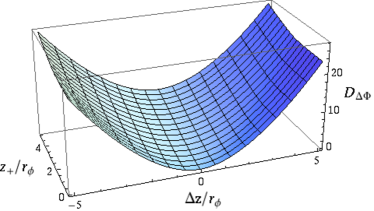
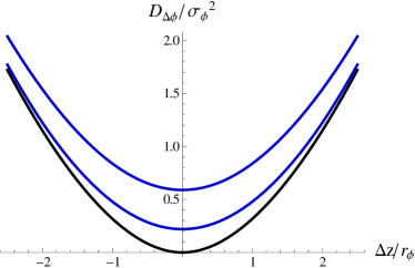
Figure 1.— Left: profile of the structure function of RM fluctuations $D_{\Delta\Phi}({\bf R},z_{1},z_{2})/(\sigma_{\phi}^{2}r_{\phi}^{2})$ in $\Delta z=z_{1}-z_{2}$ and $z_{+}=(z_{1}+z_{2})/2$ space for $R=r_{\phi}$, $m_{\phi}=2/3$. Right: cross-sections of the left panel surface at fixed $z_{+}/r_{\phi}=0,1,2$ (from lower to upper curve, respectively).

It demonstrates a valley shape with the bottom at $z_{1}=z_{2}$ line that slowly rises with $z_{+}=(z_{1}+z_{2})/2$ and steep walls in $\Delta z=z_{1}-z_{2}$ direction. Main conclusion is that the dependence in $\Delta z=z_{1}-z_{2}$ close to the local minima of $D_{\Delta\Phi}$ is primarily simply quadratic due to geometrical reason of different integration lengths.

Analytic considerations in Appendix B suggest the following quadratic approximation

$$D_{\Delta\Phi}({\bf R},z_{1},z_{2})=D_{\Delta\Phi}^{+}({\bf R},z_{+})+\frac{1}{4}(\Delta z)^{2}\Lambda_{-}(R,z_{+})$$ (19)

where along the bottom of the valley $z_{1}=z_{2}$

$$D_{\Delta\Phi}^{+}({\bf R},z_{+})=\int_{0}^{z_{+}}\!\!\!\!dz^{\prime}\!\int_{0}^{z_{+}}\!\!\!\!dz^{\prime\prime}\left(\xi_{\phi}(0,z^{\prime}-z^{\prime\prime})-\xi_{\phi}({\bf R},z^{\prime}-z^{\prime\prime})\right)=2\int_{0}^{z_{+}}dz_{-}(z_{+}-z_{-})\left(\xi_{\phi}(0,z_{-})-\xi_{\phi}({\bf R},z_{-})\right)$$ (20)

and the curvature in $\Delta z\equiv z_{1}-z_{2}$ is

$$\Lambda_{-}(R,z_{+})=\xi_{\phi}(0,z_{+})-\xi_{\phi}({\bf R},z_{+})+2\xi_{\phi}({\bf R},0)$$ (21)

The residual dependence of coefficients on $z_{+}$ is one more manifestation of inhomogeneity of statistical measures in $z$ direction. Figure 2 shows that $D_{\Delta\Phi}^{+}({\bf R},z_{+})$ as a function of $z_{+}$ is initially quadratic but then becomes linear at larger $z_{+}$. However, for $R<r_{\phi}$ both low and high $z_{+}$ asymptotics have $R$ dependence

$$D_{\Delta\Phi}^{+}(\mathbf{R},z_{+}) \sim \sigma_{\phi}^{2}\left(R/r_{\phi}\right)^{\widetilde{m}_{\phi}}z_{+}^{2}~{},\quad\quad\quad\quad\quad~{}\;R<r_{\phi}~{},\quad z_{+}\ll R~{},$$ (22)

$$D_{\Delta\Phi}^{+}(\mathbf{R},z_{+}) \sim \sigma_{\phi}^{2}R\left(R/r_{\phi}\right)^{\widetilde{m}_{\phi}}z_{+}~{},\quad\quad\quad\quad\quad R<r_{\phi}~{},\quad z_{+}\gg R~{},$$ (23)

while for $R>r_{\phi}$ at low $z_{+}$ there is no dependence on $R$ and at high $z_{+}$ $\widetilde{m}_{\phi}$ scaling is inverted

$$D_{\Delta\Phi}^{+}({\bf R},z_{+}) \sim \sigma_{\phi}^{2}z_{+}^{2}~{},~{}~{}\quad\quad\quad\quad\quad\quad\quad\quad\quad\quad R>r_{\phi},\quad z_{+}<r_{\phi}~{},$$ (24)

$$D_{\Delta\Phi}^{+}({\bf R},z_{+}) \sim \sigma_{\phi}^{2}z_{+}^{2}\left(z_{+}/r_{\phi}\right)^{-\widetilde{m}_{\phi}}~{},\quad\quad\quad\quad\quad R>r_{\phi},\quad r_{\phi}<z_{+}<R~{},$$ (25)

$$D_{\Delta\Phi}^{+}({\bf R},z_{+}) \sim \sigma_{\phi}^{2}R\left(R/r_{\phi}\right)^{-\widetilde{m}_{\phi}}z_{+}~{},~{}~{}\quad\quad\quad\quad R>r_{\phi},\quad z_{+}\gg R~{}.$$ (26)

In the subsequent sections we shall use these results extensively to analyze the asymptotics for synchrotron polarization structure functions.

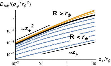
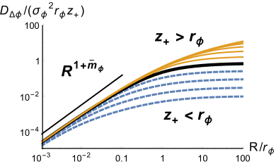
Figure 2.— $\Delta z=0$ valley bottom profile $D_{\Delta\Phi}^{+}(R,z_{+})$ Left: as the function of $z_{+}$ for several $R$ in the range from $0.001\;r_{\phi}$ to $30\;r_{\phi}$ (from bottom to the top, dashed $R<r_{\phi}$, solid $R\geq r_{\phi}$ with the thickest curve corresponding to $R=r_{\phi}$), Right: as the function of $R$ for several $z_{+}$ in the range from $0.01\;r_{\phi}$ to $1000\;r_{\phi}$ (from bottom to the top, dashed $z_{+}<r_{\phi}$, solid $z_{+}\geq r_{\phi}$ with the thickest curve corresponding to $z_{+}=r_{\phi}$),

Important special case is that of a single line-of-sight, ${\bf R}=0$. The approximation Eq. (19) is reduced to $D_{\Delta\Phi}(0,\Delta z)=\frac{1}{2}(\Delta z)^{2}\sigma^{2}_{\phi}$, demonstrating that within its range of validity Faraday effect is dominated by a purely geometrical factor, insensitive to correlations of $nH_{\|}$ quantity. We can study this case in more detail using the exact formula

$$D_{\Delta\Phi}(0,z_{1},z_{2})\equiv\frac{1}{2}\int_{z_{1}}^{z_{2}}\!\!\!\!dz^{\prime}\!\int_{z_{1}}^{z_{2}}\!\!\!\!dz^{\prime\prime}\xi_{\phi}(0,z^{\prime}-z^{\prime\prime})=\frac{1}{2}\left((\Delta z)^{2}\sigma_{\phi}^{2}-\int_{0}^{\Delta z}\!\!dz\;(\Delta z-z)D_{\phi}(0,z)\right)$$ (27)

which explicitly shows that the correlated terms are further and further subdominant to the first geometrical one as $\Delta z\equiv|z_{1}-z_{2}|$ decreases. The exact criterium is that the quadratic geometrical term dominates at $\Delta z<r_{\phi}$, where $r_{\phi}$ is the correlation length of the product of the electron density fluctuations and the parallel component of the magnetic field. At $\Delta z>r_{\phi}$ the Faraday structure function tends to another, linear, universal behaviour $D_{\Delta\Phi}(\Delta z)\propto\sigma^{2}_{\phi}r_{\phi}\Delta z$ that represents a random walk in the value of the Faraday RM accumulated over different intervals of the line-of-sight. This tendency to random walk at large $\Delta z$ is also seen in Figure 2 in the general case of separated lines-of-sight of greatly non-equal lengths. Transition for $\propto\Delta z^{2}$ to $\propto\Delta z$ behaviour depends on the details of correlation of the RM density. Note that statistics of RM fluctuations are homogeneous along a single line-of-sight.

3.3. Correlation of the synchrotron polarization at the source

Magnetic field at the source can be decomposed into regular and random components. The regular component provides mean polarization, while the random component provides fluctuations of polarization. Our study is mostly devoted to the statistical description of the random component of polarization as it is measured by the observer being averaged along the line-of-sight and rotated through Faraday rotation, although the effect of the regular magnetic field is also discussed where appropriate.

The polarization at the source provides an initial polarization in our study, which is described by polarized intensity density denoted as $P_{i}$ in this paper. As we discuss in Appendix A, polarized emissivity depends on the transverse to the line of observation magnetic field $\mathbf{H}_{\perp}$ and the wavelength $\lambda$, $j(\lambda,\mathbf{x})\propto\lambda^{\gamma-1}\left|\mathbf{H}_{\perp}\right|^{\gamma}$. In this paper we shall consider observational measures in which the underlying dependence on the wavelength is scaled out. This can be accomplished, for instance, by measuring the wavelength dependence of the mean intensity of the synchrotron radiation. Thus we consider $P_{i}(\mathbf{x})\propto\lambda^{1-\gamma}j(\lambda,\mathbf{x})$ that is wavelength independent.

Fractional power dependence on the magnetic field $\propto\left|\mathbf{H}_{\perp}\right|^{\gamma}$ is the same for the intensity and polarized intensity. This allows us to apply the results of LP12 to the polarized intensity and express the fluctuation of polarization at the source for an arbitrary index $\gamma$ using the fluctuations of magnetic field obtained for $\mathbf{H}_{\perp}^{2}$.

$$\left[\left\langle P_{i}(\mathbf{x_{1}})P_{i}^{*}(\mathbf{x_{2}})\right\rangle-\left\langle P_{i}\right\rangle\left\langle P_{i}^{*}\right\rangle\right]_{\gamma}\approx A(\gamma)\left[\left\langle P_{i}(\mathbf{x_{1}})P_{i}^{*}(\mathbf{x_{2}})\right\rangle-\left\langle P_{i}\right\rangle\left\langle P_{i}^{*}\right\rangle\right]_{\gamma=2}$$ (28)

Here $A(\gamma)$ is a factor given by the ratio of the variances $A(\gamma)=\langle P^{2}\rangle_{\gamma}/\langle P^{2}\rangle_{\gamma=2}$ which dependence on $\gamma$ is similar to that for the intensity correlations discussed in LP12. In isotropic turbulence, average polarization is zero, unless there is a uniform average component to the magnetic field. If the turbulence is anisotropic, difference between the variances of different components of the magnetic field may contribute to the mean polarization as well.

In terms of $Q$ and $U$ Stokes parameters in the observers frame, the correlation between polarizations at two sources is, in general,

$$\xi_{i}\equiv\left\langle P_{i}(\mathbf{x_{1}})P_{i}^{*}(\mathbf{x_{2}})\right\rangle=\left\langle Q(\mathbf{x_{1}})Q(\mathbf{x_{2}})+U(\mathbf{x_{1}})U(\mathbf{x_{2}})\right\rangle+i\left\langle U(\mathbf{x_{1}})Q(\mathbf{x_{2}})-Q(\mathbf{x_{1}})U(\mathbf{x_{2}})\right\rangle$$ (29)

Two parts of the correlation, real and imaginary, describe correlation invariants with respect to rotation of the observers frame. Explicit expressions via the magnetic field components for $\gamma=2$ are given in Appendix A.3. The real part is the trace of the polarization correlation matrix (see LP12) and imaginary part is the antisymmetric contribution to the correlation. For synchrotron signal, the latter one can be present only if the magnetic field correlation tensor $\left\langle H_{i}(\mathbf{x_{1}})H_{j}(\mathbf{x_{2}})\right\rangle$ has index antisymmetric part, which, in general, is related to the helical correlations (Oughton et al. 1997, also see Appendix A.3). Although we shall not consider these antisymmetric correlations in this paper, we stress that the very detection of helical correlations will be a major discovery.

The main parameters of the correlation function of the polarization at the source is the correlation length $r_{i}$ and the characteristic scaling slope $m$ of its fluctuations, and the relative contribution from the mean and fluctuating polarization. While our subsequent analysis does not rely on a specific shape of $\xi_{i}$, for numerical illustrations we adopt a saturated isotropic power law similar to Eq. (14)

$$\xi_{i}(\mathbf{X}_{1}-\mathbf{X}_{2},z^{\prime}-z^{\prime\prime})=\bar{P}_{i}^{2}+\sigma_{i}^{2}\frac{{r_{i}}^{m}}{{r_{i}}^{m}+\left(R^{2}+\Delta z^{2}\right)^{m/2}}$$ (30)

The mean polarization dominates on all scales if $\bar{P}_{i}^{2}\equiv\left\langle P_{i}\right\rangle\left\langle P_{i}^{*}\right\rangle>\sigma_{i}^{2}$, in which case the functional form for intrinsic correlation effectively corresponds to the infinite correlation length $r_{i}\to\infty$. Otherwise, the mean contribution can be neglected for separations $R<r_{i}(\sigma_{i}^{2}/\bar{P}_{i}^{2}-1)^{1/m}$ which covers all the separations within the correlation length of intrinsic fluctuations if $\bar{P}_{i}^{2}<\frac{1}{2}\sigma_{i}^{2}$.

3.4. Correlation of the observed polarization

The observed polarization is subject to both integration along the line-of-sight and to the Faraday rotation. As a result, the invariant over frame rotation measure of the observed correlation is

$$\left\langle P({\bf X_{1}},\lambda^{2}_{1})P^{*}({\bf X_{2}},\lambda^{2}_{2})\right\rangle=\int_{0}^{L}dz_{1}\int_{0}^{L}dz_{2}\left\langle P_{i}({\bf X_{1}},z_{1})P_{i}^{*}({\bf X_{2}},z_{2})e^{2i\left(\lambda_{1}^{2}\Phi({\bf X_{1}},z_{1})-\lambda_{2}^{2}\Phi({\bf X_{2}},z_{2})\right)}\right\rangle$$ (31)

We shall consider all quantities to be statistically homogeneous in real space, however we do not have homogeneity property in the square-of-wavelength “direction” $\lambda^{2}$. With the mean effect separated, Eq. (31) becomes

$$\left\langle P({\bf X_{1}},\lambda^{2}_{1})P^{*}({\bf X_{2}},\lambda^{2}_{2})\right\rangle=\int_{0}^{L}\!\!dz_{1}\int_{0}^{L}\!\!dz_{2}\;e^{2i\overline{\phi}\left(\lambda_{1}^{2}z_{1}-\lambda_{2}^{2}z_{2}\right)}\left\langle P_{i}({\bf X_{1}},z_{1})P_{i}^{*}({\bf X_{2}},z_{2})e^{2i\left(\lambda_{1}^{2}\Delta\Phi({\bf X_{1}},z_{1})-\lambda_{2}^{2}\Delta\Phi({\bf X_{2}},z_{2})\right)}\right\rangle$$ (32)

The formula represents the general expression for correlation function in PPF (position-position-frequency) data cube and is the starting point for our further study.

Observable correlation function in terms of the Stokes parameters is split again into real and imaginary parts that are separately invariant with respect to frame rotation

$$\left\langle P(\mathbf{X_{1}})P^{*}(\mathbf{X_{2}})\right\rangle=\left\langle Q(\mathbf{X_{1}})Q(\mathbf{X_{2}})+U(\mathbf{X_{1}})U(\mathbf{X_{2}})\right\rangle+i\left\langle U(\mathbf{X_{1}})Q(\mathbf{X_{2}})-Q(\mathbf{X_{1}})U(\mathbf{X_{2}})\right\rangle$$ (33)

In this paper we focus on the symmetric real part $\left\langle Q(\mathbf{X_{1}})Q(\mathbf{X_{2}})+U(\mathbf{X_{1}})U(\mathbf{X_{2}})\right\rangle$ which is easier to determine and which carries the most straightforward information about the magnetized turbulent medium. Antisymmetric imaginary part $\left\langle U(\mathbf{X_{1}})Q(\mathbf{X_{2}})-Q(\mathbf{X_{1}})U(\mathbf{X_{2}})\right\rangle$ potentially reflects helical correlations of the magnetic field, but, as will be shown, can be also generated by Faraday rotation in the anisotropic MHD turbulence. Its measurement in data provides valuable observational constraints on such contributions .

Let us summarize the parameters and scales of the problem that determine the observed synchrotron polarization correlations, subject to Faraday rotation. Long list of parameters and notations is summarized in Table 1, however not all of them determine the results independently. Our problem contains the correlation length of the rotation measure $r_{\phi}$, the correlation length of the transverse magnetic field $r_{i}$, the line-of-sight size of the emitting region $L$ and the separation between two line-of-sight $R$ over which we correlate two polarization polarization measurements. As well we have scaling slopes for RM measure $m_{\phi}$ and intrinsic correlations $m$, amplitude of fluctuations in RM $\sigma_{\phi}$ and intrinsic correlations $\sigma_{i}$, possible mean rotation $\bar{\phi}$ and mean intrinsic polarization $\bar{P}_{i}$, and the wavelength of observations $\lambda$. Among them, $\bar{P}_{i}$ is trivial to account for separately, $\sigma_{i}$ is a simple coefficient the signal is proportional to, while the magnitude of RM, either random $\sigma_{\phi}$ or mean $\bar{\phi}$ together with observation wavelength $\lambda$ determine the characteristic distance ${\cal L}_{\sigma_{\phi},\bar{\phi}}$ (see next section for exact definition) over which Faraday effect rotates the polarization by one radian. As the final tally, we have five scales, ${\cal L}_{\sigma_{\phi},\bar{\phi}}$, $r_{\phi}$, $r_{i}$, $L$, $R$ and two scaling slopes $m_{\phi}$ and $m$.

Parameter		Meaning	First appearance
Scales:
	$\lambda$	wavelength of observations	Eq.   6
	$L$	line-of-sight extent of the emitting region	Eq.   6
	$R$	separation between lines-of-sight	Eq. 14
	$r_{\phi}$	correlation length for Faraday Rotation Measure density	Eq. 14
	$r_{i}$	correlation length for polarization at the source	Eq. 30
	${\cal L}_{\bar{\phi}}$	distance of one rad revolution by random Faraday rotation	Eq. 37
	${\cal L}_{\sigma_{\phi}}$	distance of one rad revolution by mean Faraday rotation	Eq. 39
	${\cal L}_{\sigma_{\phi},\bar{\phi}}$	the smallest of ${\cal L}_{\sigma_{\phi}}$ and ${\cal L}_{\bar{\phi}}$	Eq. 38
Spectral indexes:
	$m_{\phi}$	Correlation index for Faraday RM density	Eq. 14
	$m$	Correlation index for polarization at the source	Eq. 30
Basic statistical:
	$\bar{\phi}$	Mean Faraday RM density	Eq. 9
	$\sigma_{\phi}$	rms Faraday RM density fluctuation	Eq. 10
	$\bar{P}_{i}$	Mean polarization at the source	Eq. 30
	$\sigma_{i}$	rms polarization fluctuation at the source	Eq. 30

Table 1Parameters for correlation studies of the synchrotron polarization from an extended emitting region with Faraday rotation

4. Statistics of the turbulence from single wavelength PPF slice

In this section we study how spatial correlation properties of the observed polarization of synchrotron emission reflect the underlying statistical properties of magnetic and electron density turbulence. Observed polarization correlation properties depend on the separation between the lines-of-sight and the wavelengths of the observation.

Let us consider spatial correlations in polarization maps for measurements at the fixed wavelength. Such approach we shall call Polarization Spatial Analysis (PSA). The signal is accumulated along pairs of lines-of-sight, separated by $R$. The main effect of the Faraday rotation in the sufficiently turbulent (criterium to follow) medium is to suppress the observed correlations by establishing an effective narrow line-of-sight depth over which correlated part of the signal is accumulated. As we shall show, at small separations $R<r_{\phi}$, this depth depends on $R$, resulting in modified scaling of the polarization correlations that reflects the correlation of the Faraday RM density. At large separations, the suppression is uniform, synchrotron correlations are accumulated over an effectively thin slice and reflect the underlaying correlations of the magnetic field.

We make two approximations in our quantitative treatment. First we take $\phi$ to be a Gaussian quantity, definitely good approximation when its fluctuations are dominated by the fluctuations in the magnetic field. Second, we neglect the correlations between the fluctuations in intrinsic polarization at the source $P_{i}$ and the Faraday RM. Here we note that when both are dominated by fluctuations of magnetic field, which may give the most of cross-correlation, these are different (perpendicular and parallel to line-of-sight) components of the magnetic field that define intrinsic polarization and Faraday RM. At small separations between the lines-of-sight the correlation between them is suppressed (and is formally zero along coincident lines-of-sight or between sources at the same distance when turbulence is isotropic or is a strong turbulent mix of Alfvén and slow modes as this is the case of nearly incompressible turbulence (see Goldreich & Sridhar 1995)). Whereas at large separations effect of Faraday rotation is, as we’ll see below, mostly amounts to providing a window over which synchrotron polarization fluctuations are sampled.

Under stated assumptions

$$\left\langle P({\bf X}_{1})P^{*}({\bf X}_{2})\right\rangle = \int_{0}^{L}dz_{1}\int_{0}^{L}dz_{2}\;e^{2i\overline{\phi}\lambda^{2}(z_{1}-z_{2})}\left\langle P_{i}({\bf X}_{1},z_{1})P_{i}^{*}({\bf X}_{2},z_{2})\right\rangle e^{-2\lambda^{4}\left\langle\left(\Delta\Phi({\bf X}_{1},z_{1})-\Delta\Phi({\bf X}_{2},z_{2})\right)^{2}\right\rangle}$$ (35)

$$= \int_{0}^{L}dz_{1}\int_{0}^{L}dz_{2}\;e^{2i\overline{\phi}\lambda^{2}(z_{1}-z_{2})}\xi_{i}(\mathbf{R},z_{1}-z_{2})e^{-4\lambda^{4}D_{\Delta\Phi}(\mathbf{R},z_{1},z_{2})}$$

For observations done at sufficiently long wavelength (criterium to follow), we can use quadratic approximation of Eq. (19)

$$\left\langle P({\bf X}_{1})P^{*}({\bf X}_{2})\right\rangle\approx 2\int_{0}^{L/2}dz_{+}e^{-4\lambda^{4}D_{\Delta\Phi}^{+}(R,z_{+})}\int_{-2z_{+}}^{2z_{+}}\!\!\!d\Delta z\;e^{2i\overline{\phi}\lambda^{2}\Delta z}\xi_{i}({\bf R},\Delta z)e^{-\lambda^{4}\Lambda_{-}({\bf R},z_{+})(\Delta z)^{2}}$$ (36)

According to this formulae, both the mean field and the fluctuating, turbulent Faraday rotation establish an effective width in $\Delta z$ separation over which the polarization correlations are accumulated over. For the mean field, the effective width is

$${\cal L}_{\bar{\phi}}\equiv(\lambda^{2}\bar{\phi})^{-1},$$ (37)

while the one for the fluctuative rotation is ${\cal L}_{\sigma_{\phi}}\approx(\lambda^{2}\sqrt{\Lambda_{-}})^{-1}$, both windows decreasing with the increase in the wavelength of the observations. These scales have the meaning of a line-of-sight distance over which polarization direction rotates by approximately a radian. In what follows we consider the spatial extent of the emitting region to be much larger that the smallest of these two scales, $L\gg{\cal L}_{\sigma_{\phi},{\bar{\phi}}}$, where

$${\cal L}_{\sigma_{\phi},{\bar{\phi}}}\equiv\mathrm{min}({\cal L}_{\bar{\phi}},{\cal L}_{\sigma_{\phi}}).$$ (38)

In the opposite case the effect of Faraday decorrelation can be neglected.

Note that the effect of turbulent rotation can be more dramatic, leading to Gaussian window in comparison to slower oscillatory cutoff from the mean field Faraday rotation. The quadratic approximation Eq. (36) is sufficient when this effective window produced by turbulent component of Faraday rotation ${\cal L}_{\sigma_{\phi}}$ is narrower than the intrinsic correlation length $r_{i}$ of synchrotron fluctuations arising from the magnetic field component $H_{\bot}$, i.e. when $r_{i}\lambda^{2}\sqrt{\Lambda_{-}}>1$. Following Eq. (21), $\Lambda_{-}$ is bounded from below by $2\xi_{\phi}(R,0)$, i.e $\Lambda_{-}\approx 2\sigma^{2}_{\phi}$ for $R<r_{e}$ and $\Lambda_{-}>2\sigma^{2}_{\phi}(r_{\phi}/R)^{m}$ at $R>r_{\phi}$. Thus the required criterium is $\sqrt{2}\lambda^{2}r_{i}\sigma_{\phi}>1$ with line-of-sight separation $R<(\lambda^{2}\sigma_{\phi}r_{i})^{\frac{1}{m}}r_{\phi}$. This criterium can also be written in terms of scales as $r_{i}>{\cal L}_{\sigma_{\phi}}$ and $R<(r_{i}/{\cal L}_{\sigma_{\phi}})^{1/m}r_{\phi}$ where we define

$${\cal L}_{\sigma_{\phi}}\equiv(\sqrt{2}\lambda^{2}\sigma_{\phi})^{-1},$$ (39)

which is the quantity that will be used through the rest of our paper.

4.1. Dominance of turbulent rotation, ${\cal L}_{\sigma_{\phi}}<{\cal L}_{\bar{\phi}}$

We first consider the case when $\bar{\phi}<\sigma_{\phi}$. This is the case of either weak regular magnetic field, with respect to its fluctuations, or of strongly inhomogeneous distribution of electron density, or both. The problem is complex, having five scales involved, namely the scale for Faraday rotation ${\cal L}_{\sigma_{\phi}}$, the correlation length of the rotation measure $r_{\phi}$, the correlation length of the transverse magnetic field $r_{i}$, the line-of-sight size of the emitting region $L$ and the separation between two line-of-sight $R$ over which we correlate to polarization signal. We shall always consider the extent $L$ to exceed the correlation length of the polarization fluctuations at the source, $r_{i}<L$ and we limit our studies to $R<L$. This leaves us with two parameters ${\cal L}_{\sigma_{\phi}}/r_{i}$ and $r_{\phi}/r_{i}$ to study polarization correlation as a function of $R/r_{i}$. We expect $r_{\phi}\leq r_{i}$ which in case of inequality will give rise to the intermediate regime $r_{\phi}<R<r_{i}$ which can be potentially used to investigate two correlation lengths separately. In the limiting case when polarization at the source is dominated by the mean contribution, we should replace $r_{i}$ by $L$ in all criteria and results that follow.

Now two basic regimes can be distinguished:

(a) the regime of strong Faraday rotation, ${\cal L}_{\sigma_{\phi}}<r_{i}$. In this regime, Faraday rotation does not decorrelate the polarization only from sources with $\Delta z<{\cal L}_{\sigma_{\phi}}<r_{i}$. In the approximation of Eq. (36), the integral over such narrow window of $\Delta z$ gives

$$\left\langle P({\bf X}_{1})P^{*}({\bf X}_{2})\right\rangle \sim \sqrt{\pi}\;\xi_{i}({\bf R},0)\times{\cal L}_{\sigma_{\phi}}\int_{0}^{L}\frac{dz_{+}}{\sqrt{\Lambda_{-}({\bf R},z_{+})/(2\sigma_{\phi}^{2})}}e^{-4\lambda^{4}D_{\Delta\Phi}^{+}({\bf R},z_{+})}$$ (40)

$$= \sqrt{\pi}\;\xi_{i}({\bf R},0)\times{\cal L}_{\sigma_{\phi}}W_{\phi}(R)$$

The remaining line-of-sight integral provides the effective depth along the line-of-sight $W_{\phi}$ over which the signal is accumulated. It depends on $R$ and warrants a detailed examination. For $R=0$ it evaluates simply to $L$ as $D_{\Delta\Phi}^{+}(0,z_{+})=0$ and $\Lambda_{-}(0,z_{+})=2\sigma_{\phi}^{2}$. At finite $R$, however, it is shortened, since Faraday rotation decorrelates the signal as we integrate along two non-coincident lines-of-sight. Mathematically, $D_{\Delta\Phi}^{+}(\mathbf{R},z_{+})$ increases with $z_{+}$ with coefficients that increase with $R$ as described by Eqs. (22,23, 25). To compute the Faraday effective depth, $D_{\Delta\Phi}^{+}(\mathbf{R},z_{+})$ is exponentiated and then integrated over $z_{+}$. Since $D_{\Delta\Phi}^{+}$ is growing in both $R$ and $z_{+}$, small $R$ behaviour of the $W_{\phi}(R)$ will be defined by the functional form of $D_{\Delta\Phi}^{+}(\mathbf{R},z_{+})$ at large $z_{+}$, while large $R$ dependence will be determined by small $z_{+}$. As the result the effective depth decreases with $R$

$$W_{\phi}(R)\propto{\cal L}_{\sigma_{\phi}}^{2}r_{\phi}^{\widetilde{m}_{\phi}}R^{-1-\widetilde{m}_{\phi}}~{},\quad\quad R<r_{\phi}\;\mathrm{min}\left(\left({\cal L}_{\sigma_{\phi}}/r_{\phi}\right)^{\frac{2}{2+\widetilde{m}_{\phi}}},1\right)$$ (41)

from it’s maximum value of $L$ as dictated by Eq. (23) until it becomes effectively constant $W_{\phi}\approx{\cal L}_{\sigma_{\phi}}$ (with weak dependence on $r_{\phi}$ and $m_{\phi}$) at $R\geq r_{\phi}$ as follows from Eq. (25). This behaviour of the Faraday window is summarized in Figure 3.

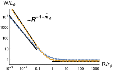
Figure 3.— Effective Faraday depth $W_{\phi}(R)$ in units of ${\cal L}_{\sigma_{\phi}}$ as the function of separation between lines-of-sight $R$ given in units of the Faraday correlation length $r_{\phi}$. Dashed lines correspond to $m_{\phi}=2/3$ and $m_{\phi}=3/2$. Solid lines are asymptotical scalings, $W_{\phi}/{\cal L}_{\sigma_{\phi}}\sim\frac{1}{4}({\cal L}_{\sigma_{\phi}}/r_{\phi})(R/r_{\phi})^{-1-\widetilde{m}_{\phi}}$ at $R\ll r_{\phi}$ and $W_{\phi}\sim\sqrt{\frac{\pi}{4m_{\phi}}}{\cal L}_{\sigma_{\phi}}$ at $R>r_{\phi}$. Here $\widetilde{m}_{\phi}=min(1,m_{\phi})$. Note that for $m_{\phi}=3/2$, the small $R$ asymptotics behaves as if $m_{\phi}=1$.

If $r_{\phi}>{\cal L}_{\sigma_{\phi}}$ one may detect the intermediate asymptotics $W_{\phi}(R)\propto{\cal L}_{\sigma_{\phi}}(r_{\phi}/R)^{m_{\phi}/2}$, over the range of scales $\left[r_{\phi}\left({\cal L}_{\sigma_{\phi}}/r_{\phi}\right)^{\frac{2}{2+\widetilde{m}_{\phi}}},r_{\phi}\right]$, as governed by Eq. (22).

Thus, at $R\ll r_{\phi}$ we have asymptotic behaviour of polarization correlation

$$\left\langle P({\bf X}_{1})P^{*}({\bf X}_{2})\right\rangle \sim {\cal L}_{\sigma_{\phi}}^{2}\xi_{i}({\bf R},0)\frac{{\cal L}_{\sigma_{\phi}}r_{\phi}^{\widetilde{m}_{\phi}}}{R^{1+\widetilde{m}_{\phi}}}\quad\quad\sqrt{2}\lambda^{2}r_{i}\sigma_{\phi}>1,\quad R<r_{\phi}$$ (42)

that is proportional to the underlying turbulent correlations taken in thin, $z=0$ slice, but is modified due to Faraday rotation by $R^{-1-\widetilde{m}_{\phi}}$. Moreover, with $r_{\phi}\leq r_{i}$ as expected, the underlying correlations are almost constant at such small separations, $\xi_{i}(R\ll r_{\phi},0)\approx\bar{P}_{i}^{2}+\sigma_{i}^{2}=const$, and $R^{-1-\widetilde{m}_{\phi}}$ scaling is the dominant one.

Whereas at larger separations, $R\gg r_{\phi}$, the correlation signal is simply accumulated from a thin slice of depth ${\cal L}_{\sigma_{\phi}}$ from the observer and the scaling of the observed polarization reflects that of the intrinsic polarization unmodified

$$\left\langle P({\bf X}_{1})P^{*}({\bf X}_{2})\right\rangle\sim{\cal L}_{\sigma_{\phi}}^{2}\xi_{i}({\bf R},0)\quad\quad\sqrt{2}\lambda^{2}r_{i}\sigma_{\phi}>1,\quad R>r_{\phi}~{}.$$ (43)

In Figure 4 we show the results of numerical integration of Eq. (35) with $\bar{P}_{i}=0$ that demonstrate the discussed regimes. It shows that the regime Eq. (43) remains valid at large $R$ even beyond the range of validity of the quadratic approximation of Eq. (36). Importantly, the change of the correlation slope is expected at $R=r_{\phi}$ which can be used to determine the RM density correlation scale $r_{\phi}$.

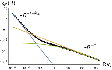
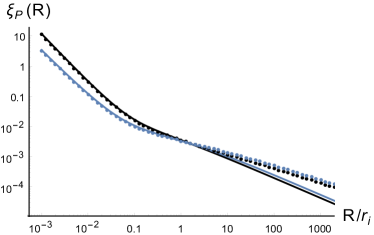
Figure 4.— The correlation function of polarization $\xi_{P}(R)\equiv\left\langle P({\bf X}_{1})P^{*}({\bf X}_{2})\right\rangle$ in the limit of strong turbulent Faraday rotation, ${\cal L}_{\sigma_{\phi}}<r_{i}$, specifically ${\cal L}_{\sigma_{\phi}}=0.07\;r_{i}$. Left: $\xi_{P}$ asymptotic regimes. Dotted line is the numerical evaluation. The correlation follows Eq. (42) at $R<r_{\phi}$ (blue) and Eq. (43) at $R>r_{\phi}$ (green). The latter regime reaches a power law behaviour for $R>r_{i}$ (orange). Here $r_{\phi}=0.1\;r_{i}$ and $\widetilde{m}_{\phi}=min(m_{\phi},1)$. Right: dependence of $\xi_{P}(R)$ on $m$ and $r_{\phi}$; $r_{\phi}=r_{i}$ (black) and $r_{\phi}=0.1\;r_{i}$ (blue); $m=2/3$ (solid) and $m=1/2$ (dotted).

We also see that in the regime of strong random Faraday rotation, 3D statistical anisotropy of the turbulence, if present, is directly mapped into 2D observational statistics via $\xi_{i}({\bf R},0)$.

(b) the weak rotation case, $r_{i}<{\cal L}_{\sigma_{\phi}}$, when the Faraday rotation is small over the distances on which intrinsic polarization is correlated. Eq. (35) asymptotically gives for observed polarization correlation

$$\left\langle P({\bf X}_{1})P^{*}({\bf X}_{2})\right\rangle\approx\int_{0}^{L}\!\!\!d\Delta z\;\xi_{i}({\bf R},\Delta z)\int_{\Delta z/2}^{L-\Delta z/2}\!\!\!dz_{+}\left(1-4\lambda^{4}D_{\Delta\Phi}(R,z_{1},z_{2})\right)$$ (44)

i.e. simply the intrinsic correlations integrated over the line-of-sight with, if the required accuracy warrants it, perturbative correction from Faraday rotation. Using the structure function, the leading behaviour at small scales is

$$\left\langle\left|P({\bf X}_{1})-P({\bf X}_{2})\right|^{2}\right\rangle \sim \sigma_{i}^{2}L^{2-\bar{m}}r_{i}^{\bar{m}}(R/R_{P})^{1+\bar{m}}=\sigma_{i}^{2}LR\left(R/r_{i}\right)^{\bar{m}}~{},\quad\bar{m}\equiv\mathrm{min}(1,m)~{},$$ (45)

where for $m<1$ the observed correlation length $R_{P}$ (defined as the scale where structure function reaches one half of its asymptotic limit $\approx L^{2-\bar{m}}r_{i}^{\bar{m}}$) depends not only on $r_{i}$, but also on the size of the emitting region,

$$R_{P}\approx r_{i}(L/r_{i})^{\frac{1-\bar{m}}{1+\bar{m}}}~{},$$ (46)

and will significantly exceed $r_{i}$ if the emitting volume extend is large, $L\gg r_{i}$. The reason is that for such low $m$ observed correlations are accumulated from pairwise volume correlations at all distance separations up to $L$. For the fixed $L$ and $r_{i}$, the larger the $m$ is, the steeper is the slope and the shorter is the correlation length of the observed correlations. For $m>1$ the observed correlation saturates at quadratic behaviour, which hides the information about the underlying turbulence. While the first expression in Eq. (45) focuses on the asymptotic value of the structure function and the observed correlation length, the second, equivalent, form reminds us that power-law asymptotics is accurate only for $R<r_{i}$. This is illustrated in Fig. 5.

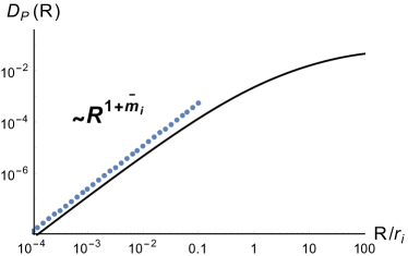
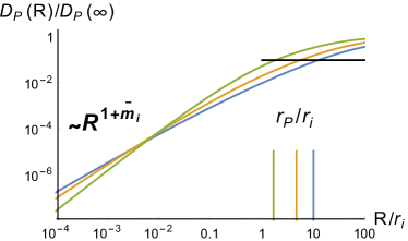
Figure 5.— The structure function of polarization $D_{P}(R)\equiv\left\langle\left|P({\bf X}_{1})-P({\bf X}_{2})\right|^{2}\right\rangle$ in the limit of negligible Faraday rotation. Depth of the emitting region is taken to be $L=100r_{i}$. Left: $D_{P}$ asymptotic regime at $R\ll r_{i}$. Solid line is the full numerical evaluation, specifically for $m=2/3$. Corresponding asymptotic slope (dotted line) is offset for clarity. Right: dependence of $D_{P}(R)$ and the observed correlation length $R_{P}$, given by Eq. (46), on $m$; $m=1/3,1/2,4/5$ – correspondingly from the longest to the shortest correlation lengths, as marked by vertical lines. According to Eq. 45, normalized structure functions intersect at $R/r_{i}\approx r_{i}/L$.

In all the regimes discussed in this section, the intrinsic correlation function $\xi_{i}$ is factorized, thus the effects from the mean intrinsic polarization and its fluctuations are additive in the observational measures. If fluctuating part is negligible, $\xi_{i}\approx\bar{P}_{i}^{2}$, one should replace $r_{i}$ by $L$ in all the above results and criteria. The only interesting case for observations is at short separations $R<r_{\phi}$ under the strong Faraday rotation, where the scaling of the Faraday rotation depth can be determined

$$\left\langle P({\bf X}_{1})P^{*}({\bf X}_{2})\right\rangle\sim{\cal L}_{\sigma_{\phi}}^{2}\bar{P}_{i}^{2}\frac{{\cal L}_{\sigma_{\phi}}r_{\phi}^{\widetilde{m}_{\phi}}}{R^{1+\widetilde{m}_{\phi}}}\quad\quad\sigma_{i}^{2}\ll\bar{P}_{i}^{2},\quad\sqrt{2}\lambda^{2}L\sigma_{\phi}>1,\quad R<r_{\phi},$$ (47)

At large separations or if the Faraday rotation is weak, the observed correlations will exhibit the plateau value, correspondent to the mean observed polarization. It can be subtracted out by measuring the structure function instead.

4.2. Dominance of the mean field in Faraday rotation, ${\cal L}_{\sigma_{\phi}}>{\cal L}_{\bar{\phi}}$

Let us now consider the situation when the RM due to the mean field is much larger than the turbulent contribution. With fluctuations in RM neglected, Eq. (35) can be rearranged as

$$\left\langle P({\bf X}_{1})P^{*}({\bf X}_{2})\right\rangle\approx 2\int_{0}^{L}\!\!\!d\Delta z(L-\Delta z)\left(\cos\left(2\overline{\phi}\lambda^{2}\Delta z\right)\xi_{i}^{e}({\bf R},\Delta z)+i\sin\left(2\overline{\phi}\lambda^{2}\Delta z\right)\xi_{i}^{o}({\bf R},\Delta z)\right)$$ (48)

where $\xi_{i}^{e}({\bf R},\Delta z)=\frac{1}{2}\left(\xi_{i}({\bf R},\Delta z)+\xi_{i}({\bf R},-\Delta z)\right)$ is the even and $\xi_{i}^{o}({\bf R},\Delta z)=\frac{1}{2}\left(\xi_{i}({\bf R},\Delta z)-\xi_{i}({\bf R},-\Delta z)\right)$ is the odd part of the intrinsic correlations with respect to $\Delta z\to-\Delta z$ change. Both parts, however, can be complex, with real part symmetric and imaginary part antisymmetric with respect to $\mathbf{r}\to-\mathbf{r}$ as has been discussed in § 3.3. So for the observable quantities

$$\left\langle Q({\bf X}_{1})Q({\bf X}_{2})+U({\bf X}_{1})U({\bf X}_{2})\right\rangle \approx 2\int_{0}^{L}\!\!\!d\Delta z(L-\Delta z)\left(\cos\left(2\overline{\phi}\lambda^{2}\Delta z\right)\Re\xi_{i}^{e}({\bf R},\Delta z)-\sin\left(2\overline{\phi}\lambda^{2}\Delta z\right)\Im\xi_{i}^{o}({\bf R},\Delta z)\right)$$ (49)

$$\left\langle Q({\bf X}_{1})U({\bf X}_{2})-U({\bf X}_{1})Q({\bf X}_{2})\right\rangle \approx 2\int_{0}^{L}\!\!\!d\Delta z(L-\Delta z)\left(\cos\left(2\overline{\phi}\lambda^{2}\Delta z\right)\Im\xi_{i}^{e}({\bf R},\Delta z)+\sin\left(2\overline{\phi}\lambda^{2}\Delta z\right)\Re\xi_{i}^{o}({\bf R},\Delta z)\right)$$ (50)

In isotropic MHD turbulence with no helical correlations, $\xi_{i}({\bf R},\Delta z)=\xi_{i}(R^{2}+\Delta z^{2})$ is even and real, thus $\Im\xi_{i}^{e}=\xi_{i}^{o}=0$, and no antisymmetric correlations should be observed

$$\left\langle Q({\bf X}_{1})Q({\bf X}_{2})+U({\bf X}_{1})U({\bf X}_{2})\right\rangle \approx 2\int_{0}^{L}\!\!\!d\Delta z(L-\Delta z)\cos\left(2\overline{\phi}\lambda^{2}\Delta z\right)\xi_{i}({\bf R},\Delta z)$$ (51)

$$\left\langle Q({\bf X}_{1})U({\bf X}_{2})-U({\bf X}_{1})Q({\bf X}_{2})\right\rangle = 0\quad.$$ (52)

Helicity in isotropic turbulence contributes only the purely odd $\Im\xi_{i}^{o}$ imaginary part and a correction to $\Re\xi_{i}^{e}$ (see Appendix A.3). Thus, despite leading to antisymmetric correlations between two emitters, it does not give rise to antisymmetric $\left\langle Q({\bf X}_{1})U({\bf X}_{2})-U({\bf X}_{1})Q({\bf X}_{2})\right\rangle$ in the observable polarization from an extended emitting region, whether Faraday rotation is present or not. It modifies the symmetric trace of the correlations only, namely

$$\left\langle Q({\bf X}_{1})Q({\bf X}_{2})+U({\bf X}_{1})U({\bf X}_{2})\right\rangle \approx 2\int_{0}^{L}\!\!\!d\Delta z(L-\Delta z)\left(\cos\left(2\overline{\phi}\lambda^{2}\Delta z\right)\Re\xi_{i}^{e}({\bf R},\Delta z)-\sin\left(2\overline{\phi}\lambda^{2}\Delta z\right)\Im\xi_{i}^{o}({\bf R},\Delta z)\right)$$ (53)

$$\left\langle Q({\bf X}_{1})U({\bf X}_{2})-U({\bf X}_{1})Q({\bf X}_{2})\right\rangle \approx 0$$ (54)

However, in contrast to the random Faraday rotation, the regular rotation can generate the observable antisymmetric correlations from anisotropy of the turbulence. For instance, for axisymmetric turbulence, the 3D correlation functions are real functions of separation magnitude $r=\sqrt{R^{2}+\Delta z^{2}}$ and the modulus of its angle with the symmetry axis $\hat{\lambda}$, $\xi_{i}=\xi_{i}(r,|\mathbf{r}\cdot\hat{\lambda}|)$. Unless the preferred direction is strictly perpendicular, $\hat{\lambda}_{z}=0$, or parallel, $\hat{\lambda}_{x}=\hat{\lambda}_{y}=0$, to the line-of-sight, such correlations, generally, contain the odd in $\Delta z$ contribution, and since $\Im\xi_{i}=0$, lead to

$$\left\langle Q({\bf X}_{1})Q({\bf X}_{2})+U({\bf X}_{1})U({\bf X}_{2})\right\rangle \approx 2\int_{0}^{L}\!\!\!d\Delta z(L-\Delta z)\cos\left(2\overline{\phi}\lambda^{2}\Delta z\right)\xi_{i}^{e}({\bf R},\Delta z)$$ (55)

$$\left\langle Q({\bf X}_{1})U({\bf X}_{2})-U({\bf X}_{1})Q({\bf X}_{2})\right\rangle \approx 2\int_{0}^{L}\!\!\!d\Delta z(L-\Delta z)\sin\left(2\overline{\phi}\lambda^{2}\Delta z\right)\xi_{i}^{o}({\bf R},\Delta z)$$ (56)

for the correlations in $Q,U$ observables.

Following the main line of the paper, let us restrict our considerations to the real, symmetric, part of the correlations as given in Eq. (51). In this problem we have four scales, ${\cal L}_{\bar{\phi}}$, $r_{i}$, $L$ and $R$. We still assume $L\gg r_{i}$, leaving us with ${\cal L}_{\bar{\phi}}/r_{i}$ parameter and $R/r_{i}$ variable. The only new regime is when Faraday rotation is strong again, ${\cal L}_{\bar{\phi}}<r_{i}$, in which case the integral is estimated as

$$\left\langle P({\bf X}_{1})P^{*}({\bf X}_{2})\right\rangle\sim L\;{\cal L}_{\bar{\phi}}\;\xi_{i}({\bf R},0)~{},\quad\quad\lambda^{2}r_{i}\bar{\phi}>1~{}.$$ (57)

This represents the behaviour similar to Eq. (43) for random RM. The difference is the absence of the effect of scale dependent RM density correlations at $R<r_{\phi}$ and the enhanced overall amplitude by $L/{\cal L}_{\bar{\phi}}$ factor. The amplitude that is $\propto(L\;{\cal L}_{\bar{\phi}})$ tells us that the observed correlation is dominated by pairs of emitters at the same (within the window ${\cal L}_{\bar{\phi}}$) line-of-sight distance, but all such pairs throughout the emitting region contribute, not just the “thin” layer closest to the observer as in the case of random Faraday rotation. To neglect any fluctuating component in the RM density is of course, an idealization. Presence of any even small, ${\cal L}_{\sigma_{\phi}}>{\cal L}_{\bar{\phi}}$, random contribution will limit the depth from which polarization correlations are coming to ${\cal L}_{\sigma_{\phi}}$. With the amplitude factored out, the behaviour of $\xi_{P}(R)$ is independent on exact value of ${\cal L}_{\bar{\phi}}/r_{i}$ and is demonstrated in Figure 6.

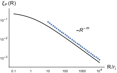
Figure 6.— The correlation function of polarization $\xi_{P}(R)=\left\langle P({\bf X}_{1})P^{*}({\bf X}_{2})\right\rangle$ in the regime of strong mean Faraday rotation, ${\cal L}_{\bar{\phi}}<r_{i}$, ${\cal L}_{\bar{\phi}}<{\cal L}_{\sigma_{\phi}}$. In this plot ${\cal L}_{\bar{\phi}}=0.1\;r_{i}$. $\xi_{P}(R)\propto\xi_{i}(R,0)$ over all range of R and is plotted with $\bar{P}_{i}=0$.

4.3. Antisymmetric correlations: illustration

We can illustrate the effect of antisymmetric correlations that arise in the presence of regular magnetic field using a simple toy model of weak anisotropy, $\xi_{i}(\mathbf{R},\Delta z)=\xi_{0}(r)\left(1+A(\mathbf{\hat{r}}\cdot\hat{\lambda})^{2}\right)$ and power-law $\xi_{0}(r)=(R^{2}+\Delta z^{2})^{-m/2}$. The odd part of 3D correlations is proportional to the degree of anisotropy

$$\xi_{i}^{o}=A\xi_{0}(r)\frac{2R\Delta z}{R^{2}+\Delta z^{2}}\sin 2\theta$$ (58)

and $\sin 2\theta$ of the angle $\phi$ between the direction of the symmetry axis and the line-of-sight. Despite relying here on a specific model, this linear in $\Delta z$ odd behaviour appears naturally in a wider context, as the first, linear term in expansion for small anisotropy. The even part of the correlation, has the main isotropic term, in addition to anisotropic correction proportional to $A\cos 2\theta$.

$$\xi_{i}^{e}=\xi_{0}(r)\left(1+{\cal O}(A\cos 2\theta)\right)$$ (59)

For our power-law $\xi_{0}(r)$ and neglecting boundary effects, Eq. (56) can be transformed by integration by parts in

$$\left\langle Q({\bf X}_{1})U({\bf X}_{2})-U({\bf X}_{1})Q({\bf X}_{2})\right\rangle \approx A\overline{\phi}\lambda^{2}R\sin 2\theta\left[2L\int_{0}^{\infty}\!\!\!d\Delta z\cos\left(2\overline{\phi}\lambda^{2}\Delta z\right)(R^{2}+\Delta z^{2})^{-m/2}\right]$$ (60)

$$\approx A\overline{\phi}\lambda^{2}R\sin 2\theta\left\langle Q({\bf X}_{1})Q({\bf X}_{2})+U({\bf X}_{1})U({\bf X}_{2})\right\rangle$$

where we have left only the leading in anisotropy term in the last expression. This result, with details depending on an exact model of turbulence, shows the main effects that determine the ratio of the imaginary antisymmetric and the real symmetric terms in the polarization correlation. They are the degree of anisotropy, amount of Faraday rotation over the distance of the separation $R$ between the two lines-of-sight, and the dependence on twice the angle between anisotropy preferred axis and the line-of-sight that makes the effect vanishing for $\theta=0$ and $\theta=\pi/2$.

Without analyzing more realistic models we may nevertheless see that the analysis of the imaginary part of the correlations can provide the information about the direction of the angle between the line-of-sight and the anisotropy preferred axis determined by magnetic field. The positional angle in the plane of the sky can be obtained either from the polarization direction or from the anisotropy measurement technique that is described in LP12. Therefore, we may state that the study of synchrotron fluctuations should provide the 3D orientation of the vector of magnetic field, which is very advantageous.

5. Line-of-sight measures

The other regime that we would like to study is the multi-wavelength observations along a fixed line-of-sight. In this section we focus on the statistical measures of polarization along a fixed line-of-sight, but at different wavelengths. Such approach that we shall call Polarization Frequency Analysis (PFA) is complimentary to PSA. Compared to the single wavelength regime, which place demands on the spatial resolution of the measurements, the regime that we study below is essentially spectroscopic, requiring sufficient wavelength resolution and coverage. We remind the reader that the basic $\lambda^{\gamma-1}$ wavelength dependence of synchrotron intensity is assumed to be scaled out in our measures.

5.1. Variance

Along a fixed line-of-sight the correlation of polarization signal measured at different wavelengths (label ${\bf X}$ can be omitted) is

$$\left\langle P(\lambda^{2}_{1})P^{*}(\lambda^{2}_{2})\right\rangle=\int_{0}^{L}dz_{1}\int_{0}^{L}dz_{2}e^{2i\overline{\phi}\left(\lambda_{1}^{2}z_{1}-\lambda_{2}^{2}z_{2}\right)}\left\langle P_{i}(z_{1})P_{i}^{*}(z_{2})e^{2i\left(\lambda_{1}^{2}\Delta\Phi(z_{1})-\lambda_{2}^{2}\Delta\Phi(z_{2})\right)}\right\rangle$$ (61)

The variance is a special case of the correlation function studied in the previous section taken at $R=0$, but it is useful to be looked at separately as a function of $\lambda^{2}$

$$\left\langle P^{2}(\lambda^{2})\right\rangle=\int_{0}^{L}\!\!\!dz_{1}\int_{0}^{L}\!\!\!dz_{2}\;e^{2i\overline{\phi}\lambda^{2}\left(z_{1}-z_{2}\right)}\left\langle P_{i}(z_{1})P_{i}^{*}(z_{2})e^{2i\lambda^{2}\left(\Phi(z_{1})-\Phi(z_{2})\right)}\right\rangle$$ (62)

and, following the discussion preceding Eq. (35)

$$\left\langle P^{2}(\lambda^{2})\right\rangle\approx\int_{0}^{L}\!\!\!dz_{1}\int_{0}^{L}\!\!\!dz_{2}\;e^{2i\overline{\phi}\lambda^{2}\left(z_{1}-z_{2}\right)}\left\langle P_{i}(z_{1})P_{i}^{*}(z_{2})\right\rangle e^{-4\lambda^{4}D_{\Delta\Phi}(0,z_{1}-z_{2})}$$ (63)

In Fig. 7 we plot the results of numerical analysis of Eq. (63) for different ratios of $\sigma_{\phi}/\bar{\phi}$ that characterizes the transition from the case when RM is predominantly stochastic to the case when Faraday rotation is mainly due to the uniform magnetic field and electron distributions.

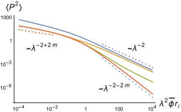
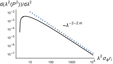
Figure 7.— Left: Polarization variance $\sigma_{P}^{2}(\lambda^{2})\equiv\left\langle PP^{*}\right\rangle$ as the function of the square of the wavelength $\lambda^{2}$. Four curves from top to bottom correspond to decreasing contribution of the turbulent component of Faraday rotation, relative to the mean field effect. The sequence is $\sigma_{\phi}/\bar{\phi}=\infty,1,0.4,0.1$. The values $\sigma_{\phi}/\bar{\phi}<0.1$ give practically the same curve as $0.1$. In case turbulent component of RM dominates, the variance scales with universal $\lambda^{-2}$ slope for $\lambda^{2}\sigma_{\phi}r_{i}>1$. In case mean RM dominates, slope of the variance reveals underlying magnetic field scaling via $\lambda^{-2-2m}$ asymptotical behaviour for $\lambda^{2}\bar{\phi}r_{i}>1$. In the regime of weak, but still present Faraday rotation, $r_{i}<{\cal L}_{\sigma_{\phi},\bar{\phi}}<L$ achieved at small wavelength, the variance shows scales as $\lambda^{-2+2m}$ for $m<1$ and saturates for $m>1$. Right: derivative of the upper curve in the right panel scales as $\lambda^{-2-2m}$ reflecting the magnetic field scaling. In both plots amplitude is in arbitrary units and $r_{\phi}=0.1\;r_{i}$.

One could expect that when Faraday window ${\cal L}_{\sigma_{\phi}}$ or ${\cal L}_{\bar{\phi}}$ is small enough to resolves $r_{i}$ it may be possible to measure the correlations of the underlying magnetic field. Our results show that situation, however, is more complicated.

One indeed recovers asymptotically the transverse magnetic field slope, if Faraday rotation is predominantly uniform $\bar{\phi}>\sigma_{\phi}$. In this case

$$\left\langle P^{2}(\lambda^{2})\right\rangle\propto\lambda^{-2-2m}~{},\quad\lambda^{2}\bar{\phi}r_{i}\gg 1~{}.$$ (64)

However when turbulent rotation dominates, $\bar{\phi}<\sigma_{\phi}$, $\left\langle P^{2}(\lambda^{2})\right\rangle$ follows the universal $\lambda^{-2}$ scaling

$$\left\langle P^{2}(\lambda^{2})\right\rangle\propto\lambda^{-2}~{},\quad\lambda^{2}\sigma_{\phi}r_{i}\gg 1~{},$$ (65)

and it is only its weighted derivative that reflects the turbulent slope of the transverse magnetic field, as shown in the right panel of Fig 7. The transition from one regime to another comes at $\sigma_{\phi}\approx\frac{1}{3}\bar{\phi}$ and is complete as $\sigma_{\phi}$ changes within the decade from $\sigma_{\phi}=0.1\;\bar{\phi}$ to $\sigma_{\phi}=\bar{\phi}$.

Our results can be understood from the following asymptotic considerations. The dominance of geometrical effects at small line-of-sight separations, as reflected in Eq. (27), allows to argue that even a simplified version of Eq. (62)

$$\left\langle P^{2}(\lambda^{2})\right\rangle=\int_{0}^{L}\!\!\!dz_{1}\int_{0}^{L}\!\!\!dz_{2}\;e^{2i\overline{\phi}\lambda^{2}\left(z_{1}-z_{2}\right)}\left\langle P_{i}(z_{1})P_{i}^{*}(z_{2})\right\rangle e^{-2\lambda^{4}\sigma^{2}_{\phi}(z_{1}-z_{2})^{2}}$$ (66)

provides a good approximation to full results as long as observations are carried out at sufficiently long wavelengths that satisfy $\lambda^{2}\sigma_{\phi}r_{\phi}>1$, i.e. ${\cal L}_{\sigma_{\phi}}<r_{\phi}$. Given the expectation that $r_{\phi}<r_{i}$, under this condition one can take $\left\langle P_{i}(z_{1})P_{i}^{*}(z_{2})\right\rangle\propto 1-\left(\frac{|\Delta z|}{r_{i}}\right)^{m}$, i.e. the variance sensitively depends on the spectral index of magnetic field $m$.

On the contrary, when Faraday rotation is dominated by the random part, $\sigma_{\phi}>\bar{\phi}$,

$$\left\langle P^{2}(\lambda^{2})\right\rangle \propto L\int_{0}^{L}\!\!\!d\Delta z(1-\Delta z/L)\left(1-\frac{\Delta z^{m}}{r_{i}^{m}}\right)e^{-2\lambda^{4}\sigma^{2}_{\phi}\Delta z^{2}}$$ (67)

$$\propto \frac{L}{\sqrt{2}\sigma_{\phi}\lambda^{2}}\left(1-\left(\sqrt{2}\lambda^{2}\sigma_{\phi}r_{i}\right)^{-m}\Gamma\left[\frac{1+m}{2}\right]/\sqrt{\pi}\right)~{},\quad\lambda^{2}\sigma_{\phi}r_{i}>1~{},$$

that shows the universal $\lambda^{-2}$ scaling which masks the decreasing with wavelength correction that is sensitive to $m$ slope index. This information is recovered in the derivative

$$\frac{\mathrm{d}\left\langle\lambda^{2}P^{2}(\lambda^{2})\right\rangle}{\mathrm{d}\lambda^{2}}=\frac{m\Gamma\left[\frac{1+m}{2}\right]}{\sqrt{\pi}}Lr_{i}\left(\sqrt{2}\lambda^{2}\sigma_{\phi}r_{i}\right)^{-1-m}$$ (68)

which, however, is more difficult to estimate from the observational data.

If most of the Faraday rotation is due to the mean distribution of $\phi=n_{e}H_{\parallel}$, $\sigma_{\phi}<\bar{\phi}$, we obtain

$$\left\langle P^{2}(\lambda^{2})\right\rangle\propto L\int_{0}^{L}\!\!\!d\Delta z(1-\Delta z/L)\left(1-\frac{\Delta z^{m}}{r_{0}^{m}}\right)\cos\left(2\overline{\Phi}\lambda^{2}\Delta z\right)\sim Lr_{i}(\lambda^{2}\bar{\phi}r_{i})^{-1-m}\frac{\sqrt{\pi}\Gamma\left[\frac{1+m}{2}\right]}{2\Gamma\left[-\frac{m}{2}\right]}$$ (69)

in the limit of large emitting area $L\gg r_{i}>{\cal L}_{\bar{\phi}}$, so the polarization variance is expected to scale with wavelength reflecting the transverse magnetic field component scaling.

Figure 7 also shows the behaviour of $\left\langle P^{2}(\lambda^{2})\right\rangle$ at small wavelength. In this case, Faraday rotation is small, ${\cal L}_{\sigma_{\phi},\bar{\phi}}>r_{i}$. Nevertheless, it still has an effect if $r_{i}\ll{\cal L}_{\sigma_{\phi},\bar{\phi}}<L$, resulting in

$$\left\langle P^{2}(\lambda^{2})\right\rangle \propto\lambda^{-2+2m}~{},\quad\quad\quad~{}~{}m<1~{},\quad\bar{\phi}>\sigma_{\phi}$$ (70)

$$\left\langle P^{2}(\lambda^{2})\right\rangle \propto\lambda^{-2-2am_{\phi}+2m}~{},\quad m<1~{},\quad\bar{\phi}<\sigma_{\phi}$$ (71)

which represents the short wavelength scaling of our expressions. When Faraday rotation is dominated by the $n_{e}H_{\parallel}$ fluctuations, their correlations steepen the shortwave scaling which is reflected in the negative $-am_{\phi}$ contribution to the slope. We have not investigated this effect in detail with asymptotic analysis, but numerical calculations show that $a\approx 1-m$ and from below the slope is limited to $\lambda^{-4}$. For $m\geq 1$ both asymptotics saturate at a constant value.

5.2. Mean polarization

For the sake of completeness, below we provide the expression for the mean polarization that arises in the presence of the mean magnetic field $\overline{H_{\perp}}$ in the volume under study. The fluctuating component of magnetic field is assumed to be present, but the directional averaging of polarization nullifies its contribution. Thus the expression for the mean polarization below is quite general:

$$\left\langle P({\bf X}_{1},\lambda^{2})\right\rangle=\int_{0}^{L}dz\left\langle e^{2i\lambda^{2}\Phi({\bf X}_{1},z)}\right\rangle=\int_{0}^{L}dze^{2i\lambda^{2}\bar{\phi}z}e^{-4\lambda^{4}D_{\Delta\Phi}(0,z)}$$ (72)

This expression assumes that the $x$ axis of the coordinate system is aligned with $\overline{H_{\perp}}$ so that there is a purely $Q$ (set to unity) uniform polarization at the source. Separately for observed $Q$ and $U$ components

$$\left\langle P_{Q}({\bf X}_{1},\lambda^{2})\right\rangle = \int_{0}^{L}dz\cos\left(2i\lambda^{2}\bar{\phi}z\right)e^{-4\lambda^{4}D_{\Delta\Phi}(0,z)}$$ (73)

$$\left\langle P_{U}({\bf X}_{1},\lambda^{2})\right\rangle = \int_{0}^{L}dz\sin\left(2i\lambda^{2}\bar{\phi}z\right)e^{-4\lambda^{4}D_{\Delta\Phi}(0,z)}$$ (74)

Eq (73) is practically identical to Eq. (63) for the variance if we replace in the latter the intrinsic correlation by a constant Thus, the mean polarization scaling can be deduced from the results for the variance by setting $m=0$ in Eqs (64,65,70,71) (due to difference between single and double line-of-sight integrals in Eq (73) and Eq. (63) there is an additional factor $L$ in resulting expressions for the variance ).

$$\left\langle P_{Q}(\lambda^{2})\right\rangle \propto\lambda^{-2}~{},\quad\quad\quad~{}\bar{\phi}>\sigma_{\phi}$$ (75)

$$\left\langle P_{Q}(\lambda^{2})\right\rangle \propto\lambda^{-2}~{},\quad\quad\quad~{}\bar{\phi}<\sigma_{\phi}~{},\quad\quad\quad\lambda^{2}\sigma_{\phi}r_{\phi}\gg 1~{},$$ (76)

$$\left\langle P_{Q}(\lambda^{2})\right\rangle \propto\lambda^{-2-2m_{\phi}}~{},\quad\bar{\phi}<\sigma_{\phi}~{},\quad\quad\quad\lambda^{2}\sigma_{\phi}r_{\phi}\ll 1~{},$$ (77)

The appearance of average $U$ polarization (in the frame oriented with magnetic field) occurs only if the mean rotation is present. Moreover, $Q$ polarization at the source rotates to be almost purely $U$ polarization at the observer if $\bar{\phi}\gg\sigma_{\phi}$, while still scaling as $\lambda^{-2}$

$$\left\langle P_{U}(\lambda^{2})\right\rangle\propto\lambda^{-2}\gg\left\langle P_{Q}(\lambda^{2})\right\rangle~{},\quad\quad\quad~{}\bar{\phi}\gg\sigma_{\phi}~{}.$$ (78)

When the mean Faraday effect is subdominant, the relative magnitude of the $U$ polarization is found numerically to change linearly

$$\frac{\left\langle P_{U}(\lambda^{2})\right\rangle}{\left\langle P_{Q}(\lambda^{2})\right\rangle}\approx A(\lambda)\frac{\bar{\phi}}{\sigma_{\phi}}~{}\,\quad\quad A(\lambda)\approx 1,~{}\quad\lambda^{2}\sigma_{\phi}r_{\phi}\gg 1~{},$$ (79)

but $A(\lambda)$ being scale dependent at small wavelengths $\lambda^{2}\sigma_{\phi}r_{\phi}<1$. The direction of the average magnetic field projected on the sky can be determined by independent techniques, e.g. via studies of the anisotropy of the intensity correlation. Then the ratio between Q and U polarization in its frame may provide the information on $\bar{\phi}$ versus $\sigma_{\phi}$.

5.3. Effect of finite resolution

Realistic observations have finite angular resolution while observing the synchrotron emission from a particular direction. This leads to averaging of the correlation signal over the beam of neighbouring lines-of-sight. Assuming isotropic sensitivity described by the beam $B$ of width $\Delta B$ in the approximation of the parallel lines-of-sight

$$P(\mathbf{X}_{1},\lambda^{2})=\int\!d\mathbf{X}\;B\left(\left|\mathbf{X}_{1}-\mathbf{X}\right|/\Delta B\right)P({\bf X},\lambda^{2})$$ (80)

To study turbulence at short scales where scaling laws are established, the experiment should obviously be able to resolve the $r_{i}$ scale, i.e., $\Delta B<r_{i}$. This, however, is not sufficient as the study of the variance of the polarization exemplifies. The generalization of the approximation Eq. (66) to finite resolution gives

$$\left\langle P^{2}(\lambda^{2})\right\rangle = 4\int_{0}^{\infty}\!\!\!RdRB^{2}(R/\Delta B)\int_{0}^{L}\!\!\!d\Delta z(L-\Delta z)\xi_{i}(R,\Delta z)\cos\left(2\overline{\Phi}\lambda^{2}\Delta z\right)e^{-4\lambda^{4}\xi_{\phi}(R)\Delta z^{2}}~{},$$ (81)

where $B^{2}(R/\Delta B)=\int\!d\mathbf{X}B\left(\left|\mathbf{X}-\frac{1}{2}\mathbf{R}\right|/\Delta B\right)B\left(\left|\mathbf{X}+\frac{1}{2}\mathbf{R}\right|/\Delta B\right)$. Its analysis shows that the scaling regimes in Eqs. (67,69) are recovered when $\Delta B<{\cal L}_{\sigma_{\phi},\bar{\phi}}$. So to summarize, the window of opportunity to recover turbulence statistics with PPF is the range of wavelengths

$$1/r_{i}<\lambda^{2}\mathrm{max}(\sigma_{\phi},\bar{\phi})<1/\Delta B~{}.$$ (82)

We remark that finite resolution does not affect the scaling of the mean polarization with the wavelength.

5.4. Faraday rotation synthesis: example of usage for turbulence study

Faraday rotation synthesis is currently becoming more popular with better frequency coverage available within PPF cubes. Below we consider how to apply our approach using the data subject to the Faraday rotation synthesis. This presentation here serves mostly to illustrate the applicability of of the synthesis within our approach to study turbulence with synchrotron fluctuations. More detailed studies of the synthesis will be provided elsewhere. In the spirit of this section we consider the Faraday rotation synthesis asymptotics for the same line of sight data while in Appendix D we provide a more general formulation of the problem.

In what follows we illustrate the use of Faraday rotation synthesis approach to studying magnetic turbulence by obtaining the Faraday rotation synthesis expression corresponding to the variance that we studied in the previous section. For this purpose we use the Eq. (D6) from Appendix D taking coinciding lines of sight, i.e. $R=0$. Along a fixed line-of-sight $\Psi_{1}-\Psi_{2}$ has the mean value $\overline{\Phi}(z_{1})-\overline{\Phi}(z_{2})=\overline{\phi}\Delta z$ and the variance $2D_{\Delta\Phi}(z_{1}-z_{2})$. Under approximation of independence of $P_{i}$ and $\Phi$ we obtain

$$\xi_{F}(0,\Psi_{1}-\Psi_{2})\approx\frac{1}{2}\int_{0}^{L}\!\!d\Delta z(L-\Delta z)\left\langle P_{i}(H_{\perp 1})P^{*}_{i}(H_{\perp 2})\right\rangle\frac{1}{\sqrt{4\pi D_{\Delta\Phi}(\Delta z)}}e^{-1/2\frac{(\Psi_{1}-\Psi_{2}-\overline{\phi}\Delta z)^{2}}{4D_{\Delta\Phi}(\Delta z)}}$$ (83)

which is an integral transform of the intrinsic polarization line-of-sight correlations. Modeling the latter, for instance, as a saturated power law $\propto\frac{\sigma_{i}^{2}r_{i}^{m}}{(r_{i}^{2}+z^{2})^{m/2}}$ shows that the dispersion function correlations recover the scaling of the underlying turbulence whether the fluctuations in Faraday RM dominate the mean or the mean is more important

$$\sigma_{\phi}>\bar{\phi}: \xi_{F}(0,\Psi_{1}-\Psi_{2})\sim\frac{L\sigma_{i}^{2}}{\sigma_{\phi}}\left(\frac{r_{i}\sigma_{\phi}}{|\Psi_{1}-\Psi_{2}|}\right)^{m-am_{\phi}}\quad\quad\Delta\Psi>r_{i}\sigma_{\phi}$$ (84)

$$\bar{\phi}>\sigma_{\phi}: \xi_{F}(0,\Psi_{1}-\Psi_{2})\sim\frac{L\sigma_{i}^{2}}{\bar{\phi}}\left(\frac{r_{i}\bar{\phi}}{|\Psi_{1}-\Psi_{2}|}\right)^{m}\quad\quad\quad\quad\Delta\Psi>r_{i}\bar{\phi}$$ (85)

The results that we obtained with the Faraday rotation synthesis are reciprocal to the results that we obtained with the variance for the regime of short wavelengths, see Eqs. (70,71). Other regimes (see Table 2) should also be possible to obtain through the Faraday rotation synthesis approach, but we do not provide the corresponding expressions in this paper.

6. Additional ways of polarimetric studies of magnetic turbulence

The formalism that we have developed allows introduction of new measures that can provide additional information about turbulence spectra and can open other ways of studying magnetic field. Some of them are discussed below.

6.1. Correlation of polarization derivative wrt $\lambda^{2}$

In this subsection we introduce a measure that is more sensitive to Faraday rotation. Combining it with the measures in the earlier subsection appears very synergetic.

Multi-wavelength Position-Position-Frequency synchrotron polarization datasets contain more information that just single-frequency sky maps or line-of-sight multi-frequency analysis that we have discussed in the previous sections. Full 3D Position-Position-Frequency analysis is beyond the scope of this paper, but a step towards utilizing frequency information in polarization maps is to study the sky correlation of the derivatives of the measured polarization wrt the (square of) wavelength $\lambda^{2}$.

$$\left\langle\frac{dP({\bf X}_{1})}{d\lambda^{2}}\frac{dP^{*}({\bf X}_{2})}{d\lambda^{2}}\right\rangle = \int_{0}^{L}\!\!dz_{1}\int_{0}^{L}\!\!dz_{2}e^{2i\overline{\phi}\lambda^{2}(z_{1}-z_{2})}\times$$ (86)

$$\times \left\langle P_{i}({\bf X}_{1},z_{1})P_{i}^{*}({\bf X}_{2},z_{2})\Delta\Phi({\bf X}_{1},z_{1})\Delta\Phi({\bf X}_{2},z_{2})e^{-2\lambda^{2}i\left(\Delta\Phi({\bf X}_{1},z_{1})-\Delta\Phi({\bf X}_{2},z_{2})\right)}\right\rangle$$

Again assuming negligible correlation between intrinsic polarization $P_{i}$ and the RM $\Phi$ we have

$$\left\langle\frac{dP({\bf X}_{1})}{d\lambda^{2}}\frac{dP^{*}({\bf X}_{2})}{d\lambda^{2}}\right\rangle = \int_{0}^{L}\!\!dz_{1}\int_{0}^{L}\!\!dz_{2}e^{2i\overline{\phi}\lambda^{2}(z_{1}-z_{2})}\xi_{i}({\bf R},z_{1}-z_{2})\left\langle\Delta\Phi({\bf X}_{1},z_{1})\Delta\Phi({\bf X}_{2},z_{2})e^{-2\lambda^{2}i\left(\Delta\Phi({\bf X}_{1},z_{1})-\Delta\Phi({\bf X}_{2},z_{2})\right)}\right\rangle$$ (87)

$$= \int_{0}^{L}\!\!dz_{1}\int_{0}^{L}\!\!dz_{2}e^{2i\overline{\phi}\lambda^{2}(z_{1}-z_{2})}\xi_{i}({\bf R},z_{1}-z_{2})\times$$

$$\times \left(\xi_{\Delta\Phi}(\mathbf{R},z_{1},z_{2})+\lambda^{4}\left(D_{\Delta\Phi}^{2}(\mathbf{R},z_{1},z_{2})-\frac{1}{4}\left(\sigma^{2}_{\Delta\Phi}(z_{1})-\sigma^{2}_{\Delta\Phi}(z_{2})\right)^{2}\right)\right)e^{-4\lambda^{4}D_{\Delta\Phi}(\mathbf{R},z_{1},z_{2})}$$

Main complexity of this result is that $\Delta\Phi$ is inhomogeneous, e.g. its variance depends on $z$ along the line-of-sight, but also its correlation functions depend on $z_{1}+z_{2}$ as well as $z_{1}-z_{2}$. Several limiting cases are tractable, but the most advantageous is to correlate the derivatives when Faraday rotation is weak, $\lambda^{4}D_{\Delta\Phi}<1$, but still non-vanishing. In this case

$$\left\langle\frac{dP({\bf X}_{1})}{d\lambda^{2}}\frac{dP^{*}({\bf X}_{2})}{d\lambda^{2}}\right\rangle \approx \int_{0}^{L}\!\!dz_{1}\int_{0}^{L}\!\!dz_{2}e^{2i\overline{\phi}\lambda^{2}(z_{1}-z_{2})}\xi_{i}({\bf R},z_{1}-z_{2})\xi_{\Delta\Phi}(\mathbf{R},z_{1},z_{2})$$ (88)

contains information about the RM as well as polarization at the synchrotron sources. This is in contrast with correlation of the polarization itself, which in the limit of weak Faraday rotation given by Eq. (44) is almost insensitive to Faraday rotation. In particular, correlating the derivatives in case of large mean component in distribution of sources, will measure the correlation of RM with asymptotical behaviour for structure function

$$\left\langle\frac{dP({\bf X}_{1})}{d\lambda^{2}}\frac{dP^{*}({\bf X}_{2})}{d\lambda^{2}}\right\rangle\propto R^{1+\widetilde{m}_{\phi}}$$ (89)

that is analogous to Eqs. (45). In general, by combining polarization and its derivative data it is potentially possible to separate the information about sources of synchrotron and RM.

In the absence of the mean magnetic field the correlation of derivatives is manifestly symmetric with respect to intrinsic and Faraday density correlations

$$\left\langle\frac{dP({\bf X}_{1})}{d\lambda^{2}}\frac{dP^{*}({\bf X}_{2})}{d\lambda^{2}}\right\rangle \approx \int_{0}^{L}\!\!dz_{1}\int_{0}^{L}\!\!dz_{2}\int_{0}^{z_{1}}\!\!dz^{\prime}\int_{0}^{z_{2}}\!\!dz^{\prime\prime}\;\xi_{i}({\bf R},z_{1}-z_{2})\xi_{\phi}(\mathbf{R},z^{\prime}-z^{\prime\prime})$$ (90)

$$= \int_{0}^{L}\!\!dz^{\prime}\int_{0}^{L}\!\!dz^{\prime\prime}\int_{0}^{z^{\prime}}\!\!dz_{1}\int_{0}^{z^{\prime\prime}}\!\!dz_{2}\;\xi_{i}({\bf R},z_{1}-z_{2})\xi_{\phi}(\mathbf{R},z^{\prime}-z^{\prime\prime})$$

It is important to note that in this measure the relative importance of contribution from the intrinsic fluctuations of polarization at the source and from turbulent Faraday rotation does not depend on how relatively strong the fluctuations are, i.e on $\sigma_{i}$ versus $\sigma_{\phi}$. It depends only on the interplay of correlation lengths $r_{i},r_{\phi}$ and scalings $m,m_{\phi}$ of the two terms.

While the line-of-sight projections in Eq. 90 complicate the discussion, much of the qualitative result can be understood by considering simply the product of the intrinsic and Faraday correlations. Let us denote

$$r_{m}\equiv\mathrm{min}(r_{i},r_{\phi}),\quad r_{M}\equiv\mathrm{max}(r_{i},r_{\phi})$$ (91)

and correspondent to $r_{m}$ and $r_{M}$ scaling indexes as $m_{m}$ and $m_{M}$ where we can have either $m_{m}\leq m_{M}$ or $m_{m}>m_{M}$ (here and below indexes $m$ and $M$ mark the terms by their respective correlation length). The product of normalized correlations $\widehat{\xi}_{i}=\xi_{i}/\sigma_{i}^{2}$ and $\widehat{\xi}_{\phi}=\xi_{\phi}/\sigma_{\phi}^{2}$ in three principal cases, (a) $r_{m}\ll r_{M}$, $m_{m}\leq m_{M}$, (b) $r_{m}\ll r_{M}$, $m_{m}>m_{M}$ and (c) $r_{m}\approx r_{M}$ is shown in Figure 8.

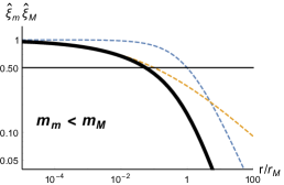
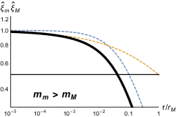
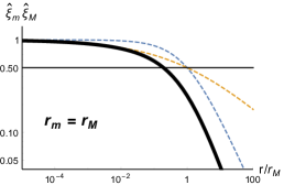
Figure 8.— Product of the two normalized correlation functions (bold solid line) versus individual terms (dashed) lines. Intersections of the dashed lines with the horizontal at $0.5$ value mark correlation lengths $r_{m}$ and $r_{M}$. Scales are given in the units of $r_{M}$, thus $r_{M}=1$. Left: the case $r_{m}\ll r_{M}$, $m_{m}<m_{M}$, here $r_{m}=0.1~{}r_{M}$, $m_{m}=1/3$ and $m_{M}=4/5$. Center: the case $r_{m}\ll r_{M}$, $m_{m}>m_{M}$, here $r_{m}=0.1~{}r_{M}$, $m_{m}=4/5$ and $m_{M}=1/3$. This plot is given in a zoomed version. Right: the degenerate case $r_{m}=r_{M}$, with $m_{m}=1/3$ and $m_{M}=4/5$.

We note two points important for the discussion: First, the combined correlation at the shortest separations follows the term with the shallowest slope. This behaviour extends until $r_{m}$ with slope $m_{m}$ in cases (a) and (c) when the shallowest correlation corresponds also to the shortest or similar correlation length, or until

$$R_{*}\approx r_{M}(r_{m}/r_{M})^{\frac{m_{m}}{m_{m}-m_{M}}}<r_{m}$$ (92)

with the slope $m_{M}$ in case (b) when the shallowest correlation has the longest correlation length. In the latter case scaling at $r_{m}>R>R*$ is determined by steeper $m_{m}$. Secondly, the presence of two effects decorrelates the signal from sources separated by large distances and as the result the overall amplitude of correlations integrated over the line-of-sight will be diminished relative to the result obtained in Eq. 45.

Let us now focus at small separations $R<r_{m}$. The short scale behaviour is best revealed in the measurements of the structure function

$$\left\langle\left|\frac{dP({\bf X}_{1})}{d\lambda^{2}}-\frac{dP({\bf X}_{2})}{d\lambda^{2}}\right|^{2}\right\rangle \approx \sigma_{i}^{2}\sigma_{\phi}^{2}\int_{0}^{L}\!\!dz_{1}\int_{0}^{L}\!\!dz_{2}\int_{0}^{z_{1}}\!\!dz^{\prime}\int_{0}^{z_{2}}\!\!dz^{\prime\prime}\times$$

$$\times \left(\left[\widehat{D}_{i}(R,\Delta z)-\widehat{D}_{i}(0,\Delta z)\right]+\left[\widehat{D}_{\phi}(R,\Delta z^{\prime})-\widehat{D}_{\phi}(0,\Delta z^{\prime})\right]\right.$$

$$- \left.\left[\widehat{D}_{i}(R,\Delta z)\widehat{D}_{\phi}(R,\Delta z^{\prime})-\widehat{D}_{i}(0,\Delta z)\widehat{D}_{\phi}(0,\Delta z^{\prime})\right]\right)$$

where $\widehat{D}\equiv D/(2\sigma^{2})$ are structure functions normalized by the correspondent variances. Since $\widehat{D}<1$, to linear order intrinsic correlations and Faraday rotation contribute additively, thus we will be comparing the full results with individual linear terms. Quadratic correction is important to understand the amplitude of the correlations.

In the first case of $m_{M}>m_{m}$ we can approximate $D_{M}(R<r_{m},z)\approx D_{M}(0,z)$ to obtain the estimate

$$\left\langle\left|\frac{dP({\bf X}_{1})}{d\lambda^{2}}-\frac{dP({\bf X}_{2})}{d\lambda^{2}}\right|^{2}\right\rangle \approx \sigma_{\phi}^{2}\sigma_{i}^{2}\int_{0}^{L}\!\!d\Delta z\widehat{D}_{m}(R,\Delta z)W_{M}(L,\Delta z)$$ (94)

$$W_{M}(L,\Delta z) \equiv \int_{\Delta z/2}^{L-\Delta z/2}\!\!dz_{p}\int_{0}^{z_{p}+\Delta z/2}\!\!dz^{\prime}\int_{0}^{z_{p}-\Delta z/2}\!\!dz^{\prime\prime}\left(1-\widehat{D}_{M}(0,\Delta z^{\prime})\right)~{}.$$ (95)

This result demonstrates that the scaling is determined by the contribution with the shortest correlation length, while the effect of the other term, compressed in $W_{M}$ window, leads to amplitude suppression relative to the uniform limit $r_{M}\to\infty$ when $W_{M}=L^{3}/3$. In detail , for $r_{M}\ll L$ we find $W_{M}\propto L^{3}(r_{M}/L)^{m_{M}}(1-\Delta z/L)^{2}$ which leads to

$$\left\langle\left|\frac{dP({\bf X}_{1})}{d\lambda^{2}}-\frac{dP({\bf X}_{2})}{d\lambda^{2}}\right|^{2}\right\rangle\propto\sigma_{i}^{2}\sigma_{\phi}^{2}L^{3}(r_{M}/L)^{m_{M}}R^{1+m_{m}}/r_{m}^{m_{m}}\quad\quad R<r_{m},\quad m_{m}\leq m_{M}~{}.$$ (96)

In the case $m_{M}<m_{m}$, however, the very short scales $R<R_{*}$ are dominated by the term with the shallowest slope, which in this case is $m_{M}$. The transition scale $R_{*}$, given above in Eq. (92), is estimated from the condition $\widehat{D}_{m}(R_{*})=\widehat{D}_{M}(R_{*})$, and is determined by the underlying correlations scales and not the size of the emitting region. Thus we have two regimes

$$\left\langle\left|\frac{dP({\bf X}_{1})}{d\lambda^{2}}-\frac{dP({\bf X}_{2})}{d\lambda^{2}}\right|^{2}\right\rangle \propto \sigma_{i}^{2}\sigma_{\phi}^{2}L^{3}(r_{m}/L)^{m_{m}}R^{1+m_{M}}/r_{M}^{m_{M}}\quad\quad R<R_{*},~{}\quad\quad\quad m_{m}>m_{M}$$ (97)

$$\propto \sigma_{i}^{2}\sigma_{\phi}^{2}L^{3}(r_{m}/L)^{m_{m}}R^{1+m_{m}}/r_{m}^{m_{m}}\quad\quad R_{*}<R<r_{m},\quad m_{m}>m_{M}$$ (98)

where the first asymptotics is obtained by setting $D_{m}(R<R_{*},z)\approx D_{m}(0,z)$ and the second one by matching at $R_{*}$. Both scalings, for intrinsic polarization at the source and Faraday rotation depth, can potentially be determined in this case. We note that while using $m$ and $M$ indexes highlights the formal symmetry between intrinsic and Faraday depth correlations in our measure, we expect the Faraday depth to have shorter correlation length, thus $r_{m}=r_{\phi}$, $r_{M}=r_{i}$ and $m_{m}=m_{\phi}$, $m_{M}=m$ is a more probable identification. In Figure 9 we illustrate the discussed regimes.

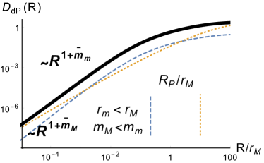
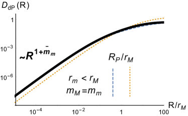
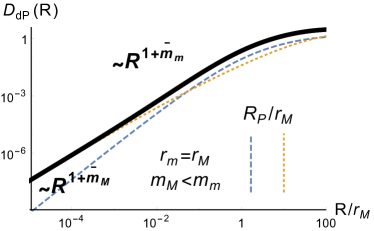
Figure 9.— Structure function of the derivative of the polarization wrt $\lambda^{2}$, $D_{dP}\equiv\left\langle\left|\frac{dP({\bf X}_{1})}{d\lambda^{2}}-\frac{dP({\bf X}_{2})}{d\lambda^{2}}\right|^{2}\right\rangle$, in units of $\sigma_{i}^{2}\sigma_{\phi}^{2}L^{3}$. Example parameters are $r_{i}=r_{M}$, $r_{\phi}=r_{m}=0.1\;r_{i}$, $L=100\;r_{i}$. Bold solid line is full result, in the left column scaled up by $(L/r_{M})^{m_{M}}$ and in the right column scaled up by $(L/r_{m})^{m_{m}}$. Individual contribution from intrinsic ($r_{M}$) and Faraday ($r_{m}$) correlations are shown by dotted and dashed lines, respectively. Vertical lines mark projected correlation lengths $R_{P}$ for the two terms. Top left: $m_{\phi}=1/3$, $m=4/5$, corresponding to the case $m_{M}>m_{m}$. For $R<r_{m}=r_{\phi}$ $D_{dP}$ scaling is determined by Faraday correlations, while for $R>r_{m}$ $D_{dP}$ follows intrinsic correlation scaling. Projected correlation scales $R_{P}$ are inverted relative to 3D ones. Top right: $m_{\phi}=4/5$, $m=1/3$, corresponding to the case $m_{M}<m_{m}$. For $R<R_{*}\approx 10^{-3}r_{i}$ $D_{dP}$ scaling is determined by intrinsic correlations, while for $R>R_{*}$ $D_{dP}$ follows Faraday correlation scaling at an enhanced amplitude. Bottom row: degenerate cases. Bottom left: $m_{\phi}=m=2/3$ corresponding to the case $m_{M}=m_{m}$. $D_{dP}$ is determined by the $r_{m}=r_{\phi}$ contribution everywhere. The difference with the top-left case is that the projected scales $R_{P}$ here follow the order of 3D correlation lengths, which is why $r_{M}$ contribution scaling is not picked up at large separations. Bottom right: $r_{i}=r_{\phi}$ case with $m_{\phi}=4/5$, $m=1/3$, which can be viewed as a continuation of the top-right case.

The result at $R>r_{m}$ has a complicated dependence on $r_{M},r_{m},m_{M},m_{m}$ and $L$, but can always be computed numerically. We notice however from Eq. (6.1) that as soon as $R$ is large enough that one of the structure functions in the integrand saturates, the quadratic correction saturates the full result. Figure 9 confirms that the contribution with the shortest projected correlation length $R_{P}$ determines the large separation behaviour and the correlation length of the polarization derivative signal .

In conclusion, measuring the correlation of the derivative of the polarization with respect to wavelength allows to study weak Faraday rotation effect. Since Faraday depth correlation can be expected to have shorter correlation lengths than intrinsic polarization, Faraday effect may be dominant in this measure, in contrast to correlating the polarization itself.

6.2. Studying turbulence with interferometric data

High resolution synchrotron maps are obtained with interferometers. To get a synthesis of interferometric data obtained for an extended range of baselines is necessary. Obtaining the interferometric measurement to fill the entire UV plane of spatial frequencies is time consuming and sometimes is impossible. At the same time, missing spatial frequencies in the data used to restore the synchrotron polarization maps can interfere with the turbulence studies and distort the output of techniques. Fortunately, as we discuss further, restoring of the synchrotron polarization image is not necessary for turbulence studies. Row interferometric data is sufficient, as we discuss below. In fact, just a few measurements with different baselines are sufficient for finding the turbulence spectra.

In the paper thus far we have discussed the use of spatial correlation functions of polarization $P$ and its derivative $dP/d\lambda^{2}$. Another way to study fluctuations is to use power spectrum:

$$S_{P}({\bf K})=\int d{\bf R}e^{\bf i{\bf KR}}\langle P({\bf X}_{1})P({\bf X}_{2})\rangle$$ (99)

where $\mathbf{R}={\bf X_{1}}-{\bf X}_{2}$. The advantage of this presentation is that $S_{P}$ can be available using raw interferometric data without requiring the full range of spatial frequencies required for restoring the distribution of polarized intensities.

Similarly, we can differentiate the observed visibilities by $\lambda^{2}$ and obtain

$$S_{dP}({\bf K})=\int d{\bf R}e^{\bf i{\bf KR}}\left\langle\frac{dP({\bf X}_{1})}{d\lambda^{2}}\frac{dP^{*}({\bf X}_{2})}{d\lambda^{2}}\right\rangle$$ (100)

As the asymptotics of $\langle P({\bf X}_{1})P({\bf X}_{2})\rangle$ and $\left\langle\frac{dP({\bf X}_{1})}{d\lambda^{2}}\frac{dP^{*}({\bf X}_{2})}{d\lambda^{2}}\right\rangle$ are known, obtaining the relations between the interferometric measurements on one hand, and the underlying magnetic field and Faraday rotation statistics on the other hand is trivial. Let us assume that $r_{\phi}\leq r_{i}$. Using Table 2 for the case of strong rotation ${\cal L}_{\sigma_{\phi},\bar{\phi}}<r_{i}$. we get for the interferometric response for the polarization fluctuations for a fixed frequency, i.e. within the PSA approach,

$$\quad{\cal L}_{\sigma_{\phi}} <{\cal L}_{\bar{\phi}} S_{P}({\bf K}) \sim K^{-1+\widetilde{m}_{\phi}}~{}, K >r_{\phi}^{-1}~{},$$ (101)

$$S_{P}({\bf K}) \sim K^{-2+m}~{}, K <r_{i}^{-1}~{}.$$ (102)

$$\quad{\cal L}_{\sigma_{\phi}} >{\cal L}_{\bar{\phi}} S_{P}({\bf K}) \sim K^{-2-m}~{}, K >r_{i}^{-1}~{},$$ (103)

$$S_{P}({\bf K}) \sim K^{-2+m}~{}, K <r_{i}^{-1}~{}.$$ (104)

Similarly using Eqs. (96), (97) and (98) for $S_{dP}$ in the regime of weak Faraday rotation we find from §6.1

$$m \geq m_{\phi} S_{dP}({\bf K}) \sim K^{-3-\widetilde{m}_{\phi}}~{}, K >r_{\phi}^{-1}~{}.$$ (105)

$$m <m_{\phi} S_{dP}({\bf K}) \sim K^{-3-\widetilde{m}_{\phi}}~{}, R_{*}^{-1}>K >r_{\phi}^{-1}~{},$$ (106)

$$S_{dP}({\bf K}) \sim K^{-3-\widetilde{m}}~{}, K >R_{*}^{-1}~{}.$$ (107)

for the case of dominance of fluctuating component and a rather trivial result that follows from Eq. (89) for the dominance of regular magnetic field

$$S_{dP}({\bf K})\sim K^{-3-\widetilde{m}_{\phi}}~{}.$$ (108)

We see that $S_{P}$ in most cases reflects the statistics of underlying magnetic turbulence that is responsible for the emission, while $S_{dP}$ is more focused on the statistics of Faraday rotation fluctuations. This corresponds to the measures of polarization that $S_{P}$ and $S_{dP}$ present spatial Fourier transforms.

We note that the measures $S_{P}(\mathbf{K})$ and $S_{dP}(\mathbf{K})$ depend also on the direction of $\mathbf{K}$ in respect to the in-plane direction of magnetic field ${\bf H}_{\bot}$. This opens ways for studying ${\bf H}_{\bot}$ direction using sparsely sampled interferometric data. In addition, as we discuss below, with such a data it is possible to study more sophisticated properties of turbulence related to its anisotropy.

6.3. Anisotropy of fluctuations

Our analysis in this paper was focused on the spectrum of the synchrotron fluctuations. The actual spectra of MHD turbulence are anisotropic. This was shown in LP12 to result in anisotropies of synchrotron fluctuations. If we compare the expression for intensity in Eq.(A8) and polarized intensity Eq.(A9) we observed that the fluctuations of the perpendicular component of magnetic field enter the same way in both expressions, i.e. they are both proportional to $\int dz|{\bf H}_{\bot}|^{\gamma}$. The difference arises from the fact that the expression for the polarization has the Faraday phase factor. In terms of correlation properties, this factor, as our analysis above shows, in most cases results in introduction of the window which limits the extent of the region from which the signal is collected. Thus the analysis of anisotropy of synchrotron fluctuations in LP12 is applicable to the correlation functions of the polarized radiation with the caveat that the magnetic field studied this way is not the magnetic field integrated over the line-of-sight through the entire emitting region, but limited by the zone extent of which determined by the Faraday window that we discussed in §4.

This provides a few new effects which are very valuable for magnetic field studies. The analysis of anisotropies in LP12 suggested that the mean magnetic field direction in the entire synchrotron -emitting region can be obtained from the analysis of the quadrupole anisotropy of the synchrotron fluctuations. In view of our earlier discussion this means that determination of the direction of magnetic field is possible within the sub volume of the synchrotron emitting region if fluctuations of polarization are studied. By changing the wavelength of the radiation one can sample the region to a different extent. This allows studying the variations of the direction of the magnetic field along the line-of-sight, which is new valuable information. In addition, LP12 found that the analysis of anisotropies can determine the relative strength of Alfvén, fast and slow modes within MHD turbulence. It is possible to see that the same analysis can be extended to obtain the variations of the corresponding strengths along the line-of-sight if polarized synchrotron emission is used for the cases when the Faraday rotation does not impose the fluctuations of its own. The latter corresponds to the limited parameter space (see left upper part of Table 2). In that special situation the analysis in LP12 should be extended.

A particular case of anisotropy analysis considered in LP12 is the case of studying anisotropies within the Milky Way when the observer is submerged in the emitting synchrotron volume. It was shown there that if the angle $\theta$ between the lines-of-sight along which the synchrotron intensity is collected is sufficiently large, i.e. $\theta$ is much larger than the ratio of the correlation radius of magnetic fluctuations $r_{i}$ to the extent of the emitting volume $L$, then the anisotropy analysis samples correlations of magnetic field only to the extent $r_{i}\theta$, which allows determining magnetic field direction variations within the emitting volume. It is easy to see that the polarization substantially extends this ability of sampling magnetic field and allows studying variations of magnetic field at scales less than $r_{i}$.

The direction of magnetic field that obtained by the correlation anisotropy analysis in LP12 will not coincide, in general, with the direction given by the mean polarization. This arises from the fact that the magnetic eddies tend to get elongated along the mean field. The latter direction is fixed in space and not affected, unlike the synchrotron polarization direction, by Faraday rotation. A comparison of the direction provided by the statistical technique above and the direction of mean polarization can provide an estimate of the mean angle of Faraday rotation for the polarized radiation.

The suggested in LP12 technique of multipole decomposition of the synchrotron radiation potentially opens ways to disentangling the contributions from compressible and incompressible motions. The spectral analysis of the fluctuations of the multipoles obtained as a result of such a decomposition opens an avenue for studies of spectra of magnetic fluctuations corresponding to compressible and incompressible motions separately. In LP12 we assumed that for our study we use single dish data or, equivalently, the interferometric data with the full coverage of spatial frequencies. Within this paper we explored a possibility of studying synchrotron with sparsely sampled interferometric data. We feel that such a data can be used within the multipole decomposition technique. We plan to elaborate the corresponding procedures elsewhere.

7. Major results and prospects of studying turbulence spectra

7.1. Starting point

This paper is the first attempt, as far as we know, to provide the detailed statistical properties of Position-Position-Frequency (PPF) data cubes of polarization data in order to study properties of underlying magnetic turbulence. Synchrotron emission is pretty complex and this probably kept theorists off the subject. For instance, its properties depend on the index of cosmic rays, as a result the intensities of both polarized and unpolarized emission depend on $H_{\bot}^{\gamma}$, where $H_{\bot}$ is the amplitude of magnetic field component perpendicular to the line of sight and $\gamma$ is related to the spectral index of cosmic rays as it is discussed in Appendix A.

This paper continues our study of the statistics of synchrotron radiation that we started in LP12. There we obtained the two point statistics of synchrotron intensities for arbitrary $\gamma$. In this paper we utilized this advance to describe the statistics of polarization in the presence of Faraday rotation. As a result, our results are applicable to a variety of situations characterized by different $\gamma$.

In LP12 we showed that the spectrum of magnetic turbulence within entire synchrotron emitting volume can be determined from synchrotron fluctuations for an arbitrary $\gamma$. The use of polarized fluctuations gives us a possibility to vary the extent of the volume under study. Indeed, we have seen in the previous sections that the Faraday rotation effect limits the extent of the region where magnetic fluctuations are being sampled.

An important finding of the present study is that we found the situations when the correlations of the polarization have imaginary parts. In other words, we found that the real part of the polarization correlations, i.e. $\left\langle Q({\bf X}_{1})Q({\bf X}_{2})+U({\bf X}_{1})U({\bf X}_{2})\right\rangle$ provides the information about the symmetric turbulence of magnetic field and electron density fluctuations, while the imaginary part, i.e. $\left\langle Q({\bf X}_{1})U({\bf X}_{2})-U({\bf X}_{1})Q({\bf X}_{2})\right\rangle$ is may not be zero and can deliver very valuable information about properties of magnetic field and turbulence. For the most part of the paper we concentrate on the real part of polarization correlations, while we briefly discuss that the non-zero imaginary part can inform us about the 3D direction of the magnetic field.

We note that for the practical analysis of the data one can use the expression $\left\langle Q({\bf X}_{1})Q({\bf X}_{2})+U({\bf X}_{1})U({\bf X}_{2})\right\rangle$ to make sure that the antisymmetric part does not contribute to the signal. In fact, this is the expression that one should identify with the analysis of the correlation of fluctuations of polarization that we discussed in the paper. Alternatively, as we discussed earlier, one can use structure functions of the polarization rather than the correlation functions. Finding that the combination $\left\langle Q({\bf X}_{1})U({\bf X}_{2})-U({\bf X}_{1})Q({\bf X}_{2})\right\rangle$ differs from zero in observations will be an important discovery. Depending on the dominant origin of the antisymmetry one can get insight either into the 3D direction of magnetic field in the emitting volume.

7.2. Polarization Spatial analysis (PSA) and Polarization Variance Analysis (PVA)

Naturally, there are different ways of studying fluctuations of polarization. In the present paper we have provided a detailed description of the study of the spatial correlations or polarization measures in spatially separated points $\left\langle P(X_{1})P(X_{2})\right\rangle$ for the same wavelength and the frequency variations of the dispersion of the polarization $\left\langle P(\lambda)\right\rangle$. The technique utilizing the former measure we termed Polarization Spatial Analysis (PSA) and utilizing the latter measure Polarization Variance Analysis (PVA). Table 2 illustrates different regimes of turbulence study that are available with the above techniques. This table also reflects the richness of the PPF data in terms of various scales that are involved and which can be recovered by the analysis of the polarization data (see also Table 1 where these scales are listed).

The variety of the scales involved arises from the fact that the resulting polarization is the outcome of both polarization of synchrotron emission collected along the line of sight and the Faraday rotation of the polarization plane. In the main text of the paper we assumed that the emission and Faraday rotation happen within the same volume. This is the most complex from the mathematical point of view situation. We consider another limiting case of separate regions of emission and Faraday rotation in Appendix C. Naturally, the intermediate cases can be presented as a superposition of these two limiting cases.

With astrophysical environments presenting us with a rich variety of different circumstances, we consider both the situation when most of Faraday rotation arises due to the turbulent field and to the mean field. The former case corresponds to turbulent decorrelation scale ${\cal L}_{\sigma\phi}$ given by Eq. (39) being smaller that the scale of Faraday decorrelation induced by mean magnetic field, i.e. ${\cal L}_{\bar{\phi}}$ given by Eq. (37). The analysis of the data allows distinguishing these two cases.

It is essential to keep in mind that ${\cal L}_{\sigma\phi}$ and ${\cal L}_{\bar{\phi}}$ are all proportional to $\lambda^{2}$ and change with the wavelength. This provides one with an opportunity to sample different volumes along the lines and use synchrotron polarization fluctuations to get unique insight into the distribution of magnetic fields and magnetic turbulence and different distances from the observer. This is the unique feature of using polarized synchrotron emission.

We deal at length with PSA and PVA techniques, as we view them as the simplest techniques involving synchrotron polarization data. At the same time, our approach is not limited to these two techniques. In fact, we also applied our approach to find a few more useful statistical measure that we discuss in the paper.

If we talk about the PSA we have several regimes. It is evident from Table 2 that for sufficiently long wavelengths the Faraday rotation effect is essential (upper left corner of Table 2, corresponding to ${\cal L}_{\sigma_{\phi}}<{\cal L}_{\bar{\phi}}$ and the separation of the lines-of-sight less than the correlation radius of $n_{e}H_{\|}$ fluctuations, i.e. $R<r_{\phi}$. In this regime the statistics of synchrotron polarization fluctuations are both affected through the presence of $\xi({\bf R},0)$ by the fluctuations of underlying perpendicular component of magnetic field $H_{\bot}$ and the fluctuations of $n_{e}H_{\|}$, which for the given example are assumed to have the spectral power law index $m_{\phi}$.

By observing the change of the scaling of the polarization fluctuations from one regime given by Eq. (42) to the other regime given by Eq. (43) which happens as the line separation $R$ becomes comparable with the correlation scale $r_{\phi}$ we can get the characteristic size of the Faraday rotation fluctuations.

In other regimes shown in Table 2 one can obtain $\xi({\bf R},0)$, i.e. to obtain the statistics of magnetic field, which is not distorted by the Faraday rotation fluctuations. Combining that with the result obtained in the regime in the upper left corner of Table 2, one can obtain also the spectral properties of the Faraday rotation fluctuations, e.g. the spectral index $m_{\phi}$.

Depending on the media the fluctuations of $n_{e}H_{\|}$ can be dominated either by electron density fluctuations or the parallel to line-of-sight component of magnetic field fluctuations. In many situations the fluctuations of magnetic field and electron density are not correlated and therefore the correlation is factorized, i.e. can be presented as a product of the electron density and magnetic field correlations. If magnetic field statistics is known through the measurements of $\xi({\bf R},0)$ as we discussed above, then in the case of no density-magnetic field correlations one can get the correlation function of electron density.

Another feature that is obvious from the analysis of Table 2 is that, apart from $r_{\phi}$, measuring of which we discussed above, we get an opportunity to obtain the characteristic correlation scales of the magnetic field $r_{i}$. If within PSA we observe at a given wavelength two regimes depending on the line-of-sight separation, then we can increase the wavelength and suppress the regime influenced by the Faraday rotation fluctuations (see upper left corner of Table 2). The transition will happen at ${\cal L}_{\sigma_{\phi},\bar{\phi}}\sim r_{i}$, which presents an interesting way to determine the correlation length of the magnetic field fluctuations.

In short, when magnetic field fluctuations dominate the Faraday rotation measure and in the case of no assumption of magnetic field and electron density correlation the PSA provides the correlation function of magnetic field and a correlation function of electron density product with magnetic field. If the magnetic field is not correlated with electron density one gets separately the correlation functions of magnetic field and electron density. The observations of the change of the polarization fluctuation slopes provide also the scales $r_{\phi}$ and $r_{i}$. In addition, by exploring the very fact that there is a change of the scalings of the polarization fluctuations (compare upper and lower lines of the left corner of Table 2) allows to establish whether the magnetic fluctuations or regular magnetic field dominate the Faraday effect. If the Faraday rotation is dominated by the regular magnetic rotation, then we have only one regime of study and all the fluctuations naturally arise from the fluctuations of the perpendicular component of magnetic field.

For the PFA, which is complementary to the PSA technique, Table 2 illustrates that the relative effect of the ratio of the mean Faraday measure to its dispersion results in rather conspicuous consequences. Indeed, the universal scaling of the variance as $\lambda^{-2}$ for long $\lambda$ testifies that the Faraday dispersion measure dominates the regular Faraday rotation. To find the underlying magnetic field spectral slope one has to differentiate the variance as it suggested by Eq. (68). Naturally, this procedure increases effects of the noise present in the data and makes recovering of the underlying turbulence statistics more involved.

At the same time, Table 2 shows that within the PFA technique one can change the wavelength to observe the change of the spectral behavior either from $\lambda^{-2}$ to $\lambda^{-2+2m}$ or from $\lambda^{-2-2m}$ to $\lambda^{-2+2m}$ and this transfer will happen at the scale ${\cal L}_{\sigma_{\phi},\bar{\phi}}\sim r_{i}$, i.e. at the correlation scale of magnetic fluctuations. It is evident that the simultaneous use of PSA and PFA increases the reliability of the results on the turbulence statistics that these techniques deliver.

	PSA, $\xi_{P}(\mathbf{R})$					PFA, $\left\langle P^{2}(\lambda^{2})\right\rangle$
	${\cal L}_{\sigma_{\phi},\bar{\phi}}<r_{i}$			${\cal L}_{\sigma_{\phi},\bar{\phi}}>r_{i}$		${\cal L}_{\sigma_{\phi},\bar{\phi}}<r_{i}$		${\cal L}_{\sigma_{\phi},\bar{\phi}}>r_{i}$
${\cal L}_{\sigma_{\phi}}<{\cal L}_{\bar{\phi}}$	$\sim{\cal L}_{\sigma_{\phi}}^{2}\xi_{i}({\bf R},0)\frac{{\cal L}_{\sigma_{\phi}}r_{\phi}^{\widetilde{m}_{\phi}}}{R^{1+\widetilde{m}_{\phi}}}$	$R<r_{\phi}$	Eq. (42)	reflects spectrum $H_{\bot}$		$\propto\lambda^{-2}$	Eq. (65)	$\propto\lambda^{-2-2am_{\phi}+2m}$	Eq. (71)
	$\sim{\cal L}_{\sigma_{\phi}}^{2}\;\xi_{i}({\bf R},0)$	$R>r_{\phi}$	Eq. (43)
${\cal L}_{\sigma_{\phi}}>{\cal L}_{\bar{\phi}}$	$\sim L\;{\cal L}_{\bar{\phi}}\;\xi_{i}({\bf R},0)$		Eq. (57)	reflects spectrum $H_{\bot}$		$\propto\lambda^{-2-2m}$	Eq. (64)	$\propto\lambda^{-2+2m}$	Eq. (70)

Table 2Different regimes of synchrotron polarization correlations in Position-Position-Frequency studies. For additional statistics see §6.

7.3. Other new ways to study turbulence

If one is interested in the Faraday rotation fluctuations, the limitation of PSA technique is that in the case of weak Faraday rotation, the statistics $\left\langle P(X_{1})P(X_{2})\right\rangle$ is only marginally sensitive to the Faraday rotation. To deal with this limitation we proposed a new measure based on the wavelength derivative of polarization $dP/d\lambda^{2}$, namely, the spatial correlations of $dP(X_{1})/\lambda^{2}$. This measure was shown to be sensitive to the fluctuations of Faraday rotation. In the case of weak Faraday rotation the asymptotic solutions are given by Eqs. (89), (96) (97) and (98), the cases for which are explained in § 6.1.

Combining the study of the statistics of $dP/\lambda$ with the statistics of $P$ in the same weak Faraday rotation regime it is possible to get separately both the statistics of underlying magnetic field and Faraday rotation. In may be worth mentioning that the latter statistics in the regime of strong Faraday rotation is important for studying the distribution of magnetic turbulence at different distances from the observer.

For the sake of simplicity, dealing with PVA and PSA techniques as well as with the statistics of $dP/d\lambda^{2}$ we did not account for the actual structure of turbulence, e.g. its anisotropy. From the point of view of power law asymptotics that we were focused on, the anisotropies of the turbulence (see e.g. §2.3) shining via synchrotron do not matter if these anisotropies do not change the spectral index. The arguments that we provided in LP12 suggest that the spectral index does not change in the global system of reference which is available through observations. This can be easily tested observationally by measuring the correlations of polarization for different fixed positional angles in the sky. If changes, in disagreement with the theory, are observed, the averaging should be performed for a fixed positional angle and all the machinery of PSA would stay intact otherwise.

The limitations for the turbulence studies related to the resolution of telescopes can be substantially mitigated with the use of interferometers. An important claim in this paper is that to get a spectrum of magnetic turbulence the full spatial frequency coverage is not necessary. In fact, measuring for a few spatial frequencies may be sufficient. The corresponding measures $S_{P}$ and $S_{d}P$ present the spatial Fourier transforms of fluctuations of $P$ and $dP/d\lambda^{2}$, respectively. The asymptotics of $S_{P}$ is given for different regimes by Eqs. (101), (102), (103), (104) and for $S_{d}P$ by Eqs. (105), (106), (107) and (108).

Within our treatment the study of turbulence using the Faraday rotation synthesis (see §5.4) has a relatively modest role. We did not see any particular advantage of using the synthesis prior to turbulence study. The obtained asymptotics are given by Eqs. (85) and (85).

Anisotropies, as we discussed earlier, are not the main focus of this paper. However, they are very informative and interesting by itself. Our study in LV99 was focused on their study for the case of unpolarized intensity. Polarized radiation opens new windows for studying the anisotropy. In other words, our research opens ways to study anisotropy in the correlation properties of $H_{\bot}$ statistics. Due to the mathematical similarity of such a problem with the one of anisotropy of synchrotron intensity fluctuations that we studied in LP12, we can directly apply the results in the aforementioned work to polarization fluctuations in the regime when the fluctuations of of $H_{\bot}$ dominate the signal (see Table 2), which for the Faraday length being less than the correlation scale of $H_{\bot}$ fluctuations, i.e. ${\cal L}_{\sigma_{\phi},\bar{\phi}}<r_{i}$, satisfies the following conditions: either ${\cal L}_{\sigma\phi}<{\cal L}_{\bar{\phi}}$ and $R>r_{\phi}$ or ${\cal L}_{\sigma_{\phi}}>{\cal L}_{\bar{\phi}}$. In the opposite regime, i.e. ${\cal L}_{\sigma_{\phi},\bar{\phi}}<r_{i}$, Table 2 testifies that the LP12 analysis is directly applicable.

As we discussed above, the change in $\lambda$ allows sampling the synchrotron emitting volume to different depths, which opens ways for the studies of distribution of magnetic turbulence within the emitting volume. This is applicable both to turbulence spectrum and to the anisotropy of magnetic turbulence. We believe that this opens a way to do tomographic analysis of the statistical properties of magnetic turbulence and distribution of magnetic fields at different distances from the observer.

We would like to stress that the condition ${\cal L}_{\sigma_{\phi},\bar{\phi}}>r_{i}$ does not mean that we return within the anisotropy analysis back to the case of intensity studies in LP12. While the aforementioned condition is fulfilled, the Faraday rotation can still determine the volume over which the anisotropies are studied.

Most of our studies are devoted to the general case of the synchrotron emitting region and Faraday rotation regions coinciding. This is the case for the synchrotron emission from the galactic disk, for instance. However, there are situations when the synchrotron emitting and Faraday rotating regions are separated in space. This is the case of the galactic synchrotron halo, which emits synchrotron polarized emission, but does not provide much of Faraday rotation due to the low concentration of thermal electrons, and galactic disk, which may provide substantial Faraday rotation. This case is simpler than the one we studied. Its results are presented in Appendix C. Observations may faces a combination of the two cases above, i.e. some synchrotron emission can be subject to Faraday rotation within the source, some can be coming from the outside and experience Faraday rotation in a localized region. With the two limiting situations quantified in our paper formalism allows modeling such situations. The variety of the measures that we described allows obtaining sufficient constraints for the corresponding numerical studies.

8. Discussion

8.1. Synchrotron statistics

Our present study and LP12 show that synchrotron statistics is very rich and important information about turbulence can be obtained. LP12 outlined perspectives for studying the direction of the mean magnetic field with synchrotron intensity as well as evaluating of the contribution from different modes. The present study employs polarization fluctuations and enables one to get the statistics of synchrotron emission and Faraday rotation at different distances from the observer as well as to estimate the 3D direction of magnetic field. We expect substantial improvements of our knowledge of the galactic and extragalactic magnetic fields from the use of the technique.

The analytical description of synchrotron fluctuations in LP12 and the present study provides an opportunity to describe synchrotron statistics for complex astrophysical situations when the emitting regions and the regions of Faraday rotation are inhomogeneous in space, magnetic field changes in the direction in respect to the line of sight. This is very important for the analysis of galactic and extragalactic synchrotron sources as well as for predicting the statistical properties of synchrotron foregrounds within CMB studies.

Our study is focused on obtaining turbulent spectra both of magnetic field and of Faraday rotation. While studying astrophysical turbulence one should take into account that the properties of turbulence may change along the line of sight and averaged rather than local properties of turbulence are available. This, however, did not prevent substantial progress in the studies of turbulent densities and velocities, as we discuss in the paper. Similarly, magnetic turbulence was also studied successfully using synchrotron intensity fluctuations (see LP12 and ref. therein). We would like to mention, however, that in terms of sampling local properties of magnetic turbulence and getting homogeneous in the statistical sense sample the suggested techniques employing synchrotron polarization have an unquestionable advantage. Indeed, using the Faraday rotation depolarization it is possible to limit the extent of the regions that contribute to the signal. This allows more localized studies of turbulence and also mitigates the problem of the sample inhomogeneity.

In our derivations we used the assumption of magnetic fields being Gaussian. Our recent numerical study (Herron et al. 2015) confirms that even for high Mach number turbulence the magnetic fields preserve Gaussian properties, which is reflected through the skewness and kurtosis calculations.

The last comment is that while the full statistical description of magnetic fields requires the use of anisotropic tensors presented in §2.3, for the limited purpose of obtaining the spectral slope of magnetic turbulence spectrum, the simplified description of turbulence that we adopted for the most part of this paper is adequate.

8.2. Relations between the parameters of the problem

For the most of the paper we consider a homogeneous volume filled with turbulent magnetic fields, relativistic electrons and turbulent thermal plasmas. We also consider in the Appendix a particular case when the thermal plasmas and the volume of synchrotron emission are separated in space. In reality, the actual picture may be a combination of the two cases.

In the present problem of studying magnetic turbulence with synchrotron polarization there are several parameters, the characteristic length of Faraday rotation arising from the mean field ${\cal L}_{\phi}$, the characteristic scale of Faraday rotation arising from the random field ${\cal L}_{\sigma}$, the correlation scale of emitting synchrotron magnetic structures $r_{i}$, the correlation scale of the Faraday rotation fluctuations $r_{\phi}$. separation between the lines-of-sight ${\bf R}$ and the size of the emitting region along the line-of-sight $L$. Both ${\cal L}_{\phi}$ and ${\cal L}_{\sigma}$ are proportional to $\lambda^{2}$. Therefore, by changing the wavelength $\lambda$ is it possible to make these sizes larger or smaller than other sizes involved in the problem. As we discussed earlier, ability to vary $\lambda$ allows to study separately the statistics of fluctuations that arise from the Faraday rotation and arising from variations of perpendicular component of magnetic field ${\bf H}_{\bot}$ responsible for synchrotron polarized emissivity.

To see correlations of synchrotron polarization it is most productive to make the measurements at $R<r_{i}$, as no appreciable correlations is expected when the sampling of independent eddies is involved. We also assumed that the thickness of emitting physical volume along the line-of-sight $L$ is much larger than the separation between the lines-of-sight $R$. This is a natural assumption for studying 3D turbulent volumes. In some particular situations of studying turbulence in thin emitting synchrotron shells, the turbulence can be essentially 2D. For such special cases our analysis can be modified accordingly.

In many cases it is natural to assume that the correlation scale of Faraday rotation fluctuations $r_{\phi}$ should be smaller than the correlation scale of the magnetic field fluctuations $r_{i}$. This is natural if fluctuations of electron density are short correlated. However, there was no particular assumption for the relation between $r_{i}$ and $r_{\phi}$ involved in our derivations.

In some astrophysical settings another parameter related to the optical depth for self-absorption of synchrotron is appropriate. However, in the present study we disregard the effect of self-absorption. This effect will be studied elsewhere.

8.3. Comparison with LP12 and relation to earlier works

All the papers on synchrotron spectra determination (see §1) prior the LP12 study used the simplifying assumption of synchrotron emissivity being proportional to the perpendicular component of magnetic field squared. This meant that the solution was suitable only for a single value of the relativistic electron spectral index. In general, synchrotron emissivity is proportional to $H_{\bot}^{\gamma}$ with $\gamma$ varying within astrophysical objects and also varying with the frequency of synchrotron radiation. This limitation was a serious constraint for the statistical studies and it was overcome in LP12.

Our present study employs the foundations established in LP12. Indeed, studying intensities as in LP12 we demonstrated that one can obtain the spectrum of magnetic fluctuations as well as the direction of the mean magnetic field along the line-of-sight. We also showed that one can find the relative importance of compressible and incompressible modes within magnetic turbulence. Intensities is the simplest emission property to study through observations and it is remarkable that a lot of information can be obtained even using synchrotron intensities alone. The polarization that we deal with in the present paper is a more sophisticated measure. The expressions for the synchrotron polarization are affected by Faraday rotation and the resulting statistics reflects both magnetic and electron density fluctuations. Naturally, for sufficiently small $\lambda$ we are getting expressions which are not affected by the Faraday rotation and the expressions for polarization become similar to those of intensity.

In terms of the analysis of the observational signal we can list a few advantages of using the polarization statistics we employ here compared to that of intensity. The most obvious advantage of the present approach is that we get another parameter that we can vary, namely, the wavelength $\lambda$. This makes the study much more informative as we discuss in §5 and §6. Additional information should be available by fitting of the model of turbulence with its injection and dissipation scales as it is done in Chepurnov et al. (2010, 2015) for the case of spectral line data. For obtaining the spectral slope of turbulence the wavelength information can increase the reliability of the measurement.

The predicted dependence on $\lambda$ is not the only advantage of using polarimetric data compared to pure intensity. The synchrotron radiation is strongly polarized and therefore polarization provides additional way to separate it from unpolarized diffuse radiation, e.g. from the free-free plasma emission. This is important, for instance, in the context of separating foregrounds in Cosmic Microwave Background studies.

In addition, as we discussed above, the advantage of using PPF data cubes is the ability of tomographic study of turbulence that the use of polarization allows. As we have demonstrated in the paper, the polarization signal is being collected from the distances limited by the Faraday depolarization effect. This allows studying turbulence at different distances from the observer.

Last, but not the least is that our study reveals the possibility of studying magnetic turbulence using wavelength information for the measurements taken along the same line-of-sight. This ability is absent for absent for the intensity data.

Our work shows the dependence on the cosmic ray spectral index affects the the polarization measures the same way that it depends intensity. We believe that our approach presents a way to extend the results to the measures that other authors (e.g. Enßlin et al. 2010) employed in the assumption of $\gamma=2$, e.g. the way to determine the “power spectrum of the magnetic tension force” (Enßlin et al. 2010) and other magnetic field statistical measures that can be obtained with synchrotron Stokes measures. Exploring these possibilities deserves a separate study.

This study provides a new approach to studies of turbulent magnetic fields. We should stress that attempts to recover statistical information about the structure of turbulent magnetic fields in the ICM from the Faraday rotation measure (RM) data (Enßlin & Vogt 2003; Vogt & Enßlin 2003, 2005; Govoni et al. 2006; Guidetti et al. 2008), as well as studies of the ISM (Haverkorn et al. 2006, 2008), and the works based on polarized synchrotron emission data (Spangler 1982, 1983, Eilek 1989a,b) can be repeated on the basis of the detailed statistical description of synchrotron polarization that we presented in LP12 and this study.

8.4. Statistics of PPV and PPF data cubes

Our present paper presents the description of the statistics of synchrotron fluctuations in the PPF space. The corresponding description of the statistics of spectral line fluctuations in the Position-Position-Velocity (PPV) space was provided in Lazarian & Pogosyan (2000, 2006). We see both similarities and differences of the aforementioned statistics. We can observe that while the PPV statistics is strongly influenced by both the fluctuations of density and velocity, the statistics of fluctuation in the PPF arise from the fluctuations of magnetic field and those in Faraday rotation. The latter is affected by the product of electron density and parallel component of magnetic field. Thus in both cases we deal with a signal that is affected by different turbulent fields.

At the same time, the properties of PPF and PPV data cubes are different. In PPV cubes we could separate the contributions from velocity and density by changing the thickness of the frequency intervals over which we sampled the cube, i.e. by changing the thickness of velocity slices. In PPF cubes, for a given spatial separation of the correlated points, the low frequency part of PPF depending on the regime (see Table 2) is dominated by both the Faraday rotation fluctuations and fluctuations of magnetic field or just fluctuations of magnetic field, while the higher frequency part of PPF cube arises from only magnetic fluctuations. In other words, the ways of extracting statistical information from PPV and PPF are different. By studying PPF at sufficiently high frequencies the information about $H_{\bot}$ can be obtained, which if combined with the statistics at low frequencies provides the information about $nH_{\|}$. Important difference between the PPV and PPF statistics is that PPV statistics is homogeneous in the velocity direction, while PPF statistics is strongly inhomogeneous. This provides additional information about turbulent volumes. For instance, changing the wavelength it is possible to explore regions at different distances from the observer. This is a capability not available with PPV data cubes. In addition, anisotropy in PPF results in additional effects unique for this space, e.g. in the imaginary part of correlations as it is discussed in §4.3.

Integration over a range of frequencies, or frequency resolution play an important role for VCA, but it is not so important within the PSA if the range of frequencies is within one of the distant regimes of $nH_{\|}$ or $H_{\bot}$ integration (see Figure 3). If, however, the power is integrated over the frequencies includes the range of the transition from one asymptotic regime to another, the resulting behavior will not reflect any of the asymptotics.

Our PFA technique can be considered as the analog of the VCS technique that we developed for the PPV space. Similarly to VCS, this technique does not use spatial information to get the statistics of turbulence. Therefore, we expect that, similar to the VCS, the new technique can get the statistics of turbulence using measurements just along 5-10 lines-of-sight. The latter was established numerically in Chepurnov & Lazarian (2010).

In the paper we were focused on the asymptotic regimes. In this respect our study follows the theoretical approach in our papers dealing with obtaining velocity turbulence using Doppler shifted spectroscopic data (Lazarian & Pogosyan 2000, 2006). However, we also obtained general expressions for the synchrotron polarization in the presence of Faraday rotation. Our corresponding general expressions obtained for the spectroscopic data were used in the study of Chepurnov et al. (2010) to provide a detailed description of turbulence, including In particular, studying HI emission with GALFA data Chepurnov et al. (2010) provided not only slopes of the underlying velocity and density fluctuations, but also the injection scale and other parameters. The fruitfulness of such an approach was shown in the subsequent study by Chepurnov et al. (2015) that revealed that the corresponding properties of turbulence in Small Magellanic Cloud are rather different from those in our galaxy. We feel that a similar approach can be fruitful within our new technique synchrotron polarization technique described in the present paper.

8.5. Variations of cosmic rays distribution

The fact that the expression for synchrotron intensity depends on the spectral index of cosmic rays has been an impediment for the quantitative studies of the statistics of synchrotron variations. Our study shows that cosmic ray spectral variations change only the amplitude of the polarization fluctuation that we discussed. As varying $\lambda$ allows to sample synchrotron emitting regions to different depths, we may encounter the variations of spectral index in the sampled regions. Then the use the correction factors from LP12 can be employed, if necessary.

Our study has been performed in the assumption of no magnetic field correlation with the density of relativistic electrons. This assumption corresponds to observation of much smoother distribution of relativistic electrons compared to the distribution of magnetic fields in the Milky Way. Our formalism, however, may be extended for the case of relativistic electrons correlated with magnetic fields. We do not expect substantial changes in our present conclusions, e.g. in the dependence of synchrotron intensity spectrum on $\gamma$.

8.6. Galaxy and extragalactic sources

With the enhanced resolution of the synchrotron data available it is possible to apply our techniques not only to Milky Way, but also to extragalactic sources, e.g. to nearby galaxies and radio lobes of radio galaxies. For such extragalactic applications, the synchrotron radiation and Faraday rotation of Milky Way acts as a foreground. Incidentally, the usage of the raw interferometric data in order to obtain turbulent spectra is most advantageous for this application as getting turbulence spectra would not require full spectral frequency coverage.

For the two techniques the Milky Way foreground acts differently. It is influence is strongest to the PFA one as the information is collected along a single line-of-sight. For the PSA, if the angular extent of the synchrotron source is relatively small, then the influence of the Milky Way amounts to essentially constant along both lines-of-sight Faraday rotation and synchrotron polarization intensity. Those should not interfere with the analysis. As a result we expect that the technique can study the distribution of turbulence in extragalactic sources.

For the turbulence anisotropy analysis the variations of the Milky way polarization for the beams separated at distances much smaller than $r_{i}$ are expected to be small. Therefore the variations are expected to arise mostly from an extragalactic source and the anisotropy analysis should reveal the magnetic field and its variations within the source.

8.7. Synergetic use of different techniques

Galactic data synchrotron emission presents a natural object for studying with the new technique. However, the technique can be used to measure the statistics of distant objects, e.g. external galaxies and clusters of galaxies as the resolution of instruments increases.

Magnetic fluctuations that are available through the study of PSA and PSF techniques described above are very important for understanding both the fundamental properties of MHD turbulence and its influence on key astrophysical processes, e.g. star formation (see McKee & Ostriker 2007) and cosmic ray propagation (see Schlickeiser 2002, Yan & Lazarian 2008), as well as for the mapping of the sources and sinks of turbulent energy. The synchrotron fluctuations deliver the information on magnetic fluctuations, which is complementary to the velocity statistics that is available by other techniques. The currently alternative way of studying magnetic fluctuations is through using dust polarization signal, which is a technique that is limited by our the ability of dust grains to follow magnetic fields and the uncertainties of the grain alignment theory (see Lazarian 2007 for a review).

The VCA and the VCS techniques that we developed for the analysis of the velocity fluctuations provide the statistics of velocity fluctuations. In MHD turbulence, the velocity and magnetic field statistics are related and therefore the simultaneous use of the two measures is advantageous. In addition, the measures may be very complementary, as spectral lines and velocities may sample different regions along the line-of-sight.

In general, in the presence of the complex, inhomogeneous ISM it is really advantageous to use complementary statistical measures which can provide a better insight into the complexity of the turbulence. Thus combining velocity and magnetic field is synergetic.

In addition to velocity that we can obtain with e.g. VCA and VCS techniques we can use the statistics of density. Those can be obtained using some of the new techniques that have been developed recently. Those include the analysis of moments of the density probabilities (Kowal et al. 2007, Burkhart et al. 2009, 2010), Tsallis statistics (Esquivel & Lazarian 2010, Tauffmire et al. 2011), bispectra and genus (Lazarian 1999, Chepurnov et al. 2008, Burkhart et al. 2009) etc.

Apart for analyzing the density, the aforementioned techniques can be applied to the synchrotron emission distributions. For instance, in Burkhart et al. (2012) used kurtosis, skewness and genus of the polarized intensity gradient distribution to establish the Mach number of turbulence. Such work provides complementary information about the properties of magnetic turbulence under study. We note that the general formalism describing fluctuations of polarization that we developed in this paper can be modified for study spectra of gradients of polarization and the anisotropy of the gradients of polarization. The advantages of using of gradients, e.g. utilizing interferometric data which does not contain single dish observations, are described in Gaensler et al. (2011).

8.8. Utility of the information available

The techniques described above outline new ways of studying anisotropic astrophysical magnetic turbulence both in Milky Way and beyond. The injection and dissipation scales as well as spectral slope of magnetic turbulence provide keys to addressing many problems of turbulence. These properties are necessary for studying cosmic ray transport and cosmic ray acceleration, as well as studying heat and mass transport in astrophysical environments. In addition, studies of turbulence anisotropy open ways for studying turbulence compressibility. Combined with statistical studies of density and velocity, the new techniques allow ways to identify sources of turbulence in different phases of interstellar media over the range of scales from kiloparsecs to astronomical units. The corresponding knowledge is necessary for a wide range of subjects from star formation to interstellar chemistry.

We note, that the interest to properties of magnetic turbulence in Milky Way also arises from its role of inducing fluctuations of foreground radiation. In particular, we discussed potential ways of removing foregrounds if the spectrum of turbulence is known. The application of such an approach for CMB data is discussed in Cho & Lazarian (2010) and for high redshifted atomic hydrogen emission in Cho, Lazarian & Timbie (2012). Last but not the least, the information about turbulence obtained through observations is important for understanding of the enigmatic nature of MHD turbulence.

8.9. Future work

The present paper presents the first to our knowledge detailed statistical description of the synchrotron polarization fluctuations. It capitalizes on our study in LP12, which provided the description of fluctuations for an arbitrary index of cosmic rays. However, this work does not address all the questions. While it provides analytical expressions of the different regimes of the PSA and PFA studies, it explores analytically only one regime of turbulence study within the Faraday rotation synthesis. Naturally, the corresponding work should be extended.

We have noticed in the present paper that the helical correlations should result in distinct signature, making the correlation function of polarization (see Eq. (32) complex. The second term in Eq. (32) contains the valuable information about 3D direction of magnetic field and therefore this term deserves a separate theoretical study.

The effects of self-adsorption is neglected within our treatment. This effect may be important for some data sets and also should be accounted for in future. Our experience with PPV data cubes in Lazarian & Pogosyan (2004) show that absorption can substantially change the observed statistics. Fortunately, effects of self absorption are less common in synchrotron compared to the spectroscopic data.

9. Summary

Motivated by the richness of the synchrotron data available with operating telescopes and the prospects of higher resolution and sensitivity that is going to be available for synchrotron observations in the near future, we proceed with our studies of synchrotron fluctuations Our present study capitalizes on our previous investigation in LP12, which established the way to describe synchrotron fluctuations for the arbitrary index of cosmic ray spectrum. Unlike the LP12 it is aimed on using synchrotron polarization rather than intensity. Synchrotron polarization fluctuations carry information both about the statistics of random magnetic field perpendicular to the line-of-sight as well as of the fluctuations of the product of the electron density and the parallel component of magnetic field. Obtaining these statistics from the statistics of synchrotron polarization fluctuations was our goal in the paper. Within the assumptions discussed throughout the paper we have obtained analytical results which can be briefly summarized in the following way:

• We provided an analytical description of the statistics of synchrotron polarization fluctuations within Position-Position-Frequency (PPF) data cubes and employed this description to develop two complementary techniques to study the spectra of the underlying fluctuations of magnetic field and electron density.

• The first technique that we termed Polarization Spatial Analysis (PSA) employs the correlations of the polarization intensities measured at the same frequency. At high frequencies it samples $H_{\bot}$ fluctuation, while at lower frequencies the technique is also sensitive to the fluctuations of $n_{e}H_{\|}$ measure, provided that these fluctuations dominate Faraday rotation arising from the regular field. We find that the PSA is a powerful technique that can provide the spectrum of magnetic fluctuations, the slope of Faraday rotation fluctuations, the correlation scale of Faraday rotation fluctuations, the correlations scale or magnetic turbulence fluctuations as well as to give insight into the ratio of the regular and random magnetic fields.

• The second technique that we termed Polarization Frequency Analysis (PFA) employs the change of the variance of polarization with frequency. The properties of the variance as a function of frequency were found to depend on whether the rotation measure is dominated by the regular Faraday rotation arising from the mean field or the Faraday rotation is dominated by $n_{e}H_{\|}$ fluctuations. In the former case the dependence of the variance of polarization on frequency reflects the statistics of $H_{\bot}$. In the latter case the variance of polarization exhibits a universal asymptotic but we suggest a measure that uses the derivative of the variance and which reflects the $H_{\bot}$ statistics. By studying the change of the slope one also can determine the correlation length of magnetic field fluctuations.

• Polarization fluctuation are predicted to exhibit anisotropy that arises from the MHD turbulence anisotropy. The technique for such a study is similar to the one in LP12 but has the advantage that the sampling distance along the lines-of-sight can be controlled by changing the wavelength of the radiation. This allows to study the variations of the regular magnetic field along the line-of-sight.

• The imaginary part of the correlation functions of polarization contains the information about the 3D direction of mean magnetic field, which is a very valuable information to be obtained from the PPF studies.

• Our analysis of the effects of the spatial and frequency resolution of the telescopes provides the criteria for the averaging that the finite resolution involves not to distort the results obtained with the techniques.

• We introduced a new measure of polarization statistics $\left\langle\left|\frac{dP({\bf X}_{1})}{d\lambda^{2}}-\frac{dP({\bf X}_{2})}{d\lambda^{2}}\right|^{2}\right\rangle$ which we found is more sensitive to Faraday rotation and therefore is complementary to the polarization correlations used with PSA technique.

• We showed that interferometers can be used directly to study magnetic turbulence and provided the corresponding asymptotics. This extends the possibilities of using synchrotron for studying turbulence in different astrophysical objects, including external galaxies.

Appendix A Synchrotron intensity and synchrotron polarization

A.1. Basics

Synchrotron emission arises from relativistic electron spiraling about magnetic fields. The emission has been discussed in many monographs (see Pacholczyk 1970, Fleishman 2008 and references therein). Careful study of the formation of the synchrotron signal (see Westfold 1959) revealed that the signal is essentially non-linear in the magnetic field $H$ ($B$). The origin of nonlinearity is in relativistic effects. Nonlinearity comes from the fact that the signal is formed only over the narrow fraction of the electron cycle, and the two leading orders in the deviation of the trajectory from the straight line give the same contribution in terms of the inverse of the Lorentz factor $1/\gamma_{L}$. Summation of the result over “flashes” is also non-straightforward, and produces spread frequency spectrum (Westfold 1959). Situation is remarkably different from cyclotron (non relativistic) emission where emission is monochromatic and has intensity just quadratic in the magnetic field.

If the distribution of relativistic electrons in terms of the Lorentz factor is

$$N_{re}(\gamma_{L})d{\gamma_{L}}=N_{0}{\gamma_{L}}^{-p}d{\gamma_{L}}$$ (A1)

where $N_{0}$ is a normalization constant proportional to the density of relativistic electrons and $p$ is the spectral index of the electron distribution, then the observer sees intensity of the synchrotron emission

$$I_{sync}({\bf X})\propto\int dzH_{\perp}^{\gamma}({\bf x})$$ (A2)

where ${\bf X}=(x,y)$ is the 2D position vector on the sky and $H_{\perp}=\sqrt{H_{x}^{2}+H_{y}^{2}}$ is the magnitude of the magnetic field perpendicular to the line-of-sight $z$. Note that $\gamma=\text@frac{1}{2}(p+1)$ is, generally, a fractional power.

The linearly polarized radiation can be characterized by two directional intensities $I^{x}$, $I^{y}$ and the angle of polarization $\xi^{xy}$ that are connected to the Stokes parameters as (see Pacholczyk 1970):

$$I=I^{x}+I^{y}~{},\quad Q=I^{x}-I^{y}~{},\quad U=(I^{x}-I^{y})\mathrm{tan}2\xi^{xy}$$ (A3)

The subject of the LP12 study was the properties of intensity $I$, while the present study is focused on the polarization $Q$ and $U$. In the frame aligned with the direction of $\mathbf{H}_{\perp}$ only Q is present. It is convenient to subdivide the emissivity into two components, respectively perpendicular and parallel to $\mathbf{H}_{\perp}$ (see Rybicki & Lightman 1979)

$$j_{\perp}(\omega,\mathbf{x}) = \left[F(p)+G(p)\right]\omega^{(1-p)/2}|\mathbf{H}_{\perp}(\mathbf{x})|^{\gamma}$$ (A4)

$$j_{\parallel}(\omega,\mathbf{x}) = \left[F(p)-G(p)\right]\omega^{(1-p)/2}|\mathbf{H}_{\perp}(\mathbf{x})|^{\gamma},$$ (A5)

where $\omega=2\pi c/\lambda$, $\lambda$ is the observation wavelength, $c$ is the speed of light, and

$$F(p) = \frac{\sqrt{3\pi}\,e^{3}}{32\pi^{2}m_{e}c^{2}}\left(\frac{2m_{e}c}{3e}\right)^{(1-p)/2}N_{0}\,\Gamma\left(\frac{p}{4}-\frac{1}{12}\right)\frac{2^{(p+1)/2}}{p+1}\Gamma\left(\frac{p}{4}+\frac{19}{12}\right)\frac{\Gamma\left(\frac{p}{4}+\frac{5}{4}\right)}{\Gamma\left(\frac{p}{4}+\frac{7}{4}\right)},$$ (A6)

$$G(p) = \frac{\sqrt{3\pi}\,e^{3}}{32\pi^{2}m_{e}c^{2}}\left(\frac{2m_{e}c}{3e}\right)^{(1-p)/2}N_{0}\,\Gamma\left(\frac{p}{4}-\frac{1}{12}\right)2^{(p-3)/2}\Gamma\left(\frac{p}{4}+\frac{7}{12}\right)\frac{\Gamma\left(\frac{p}{4}+\frac{5}{4}\right)}{\Gamma\left(\frac{p}{4}+\frac{7}{4}\right)},$$ (A7)

where $m_{e}$ is the electron mass, $e$ is its charge, and $N_{0}$ is the prefactor of the electron distribution (Eq. (A1)). Then, the specific intensity ${\rm I}$ and the polarized specific intensity ${\rm PI}=Q+iU$ are (see Waelkens et al. 2009)

$${\rm I}(\omega,\mathbf{X}) = \int_{b}^{a}dz\left[j_{\perp}(\omega,\mathbf{x})+j_{\parallel}(\omega,\mathbf{x})\right],$$ (A8)

$${\rm PI}(\omega,\mathbf{X}) = \int_{b}^{a}dz\left[j_{\perp}(\omega,\mathbf{x})-j_{\parallel}(\omega,\mathbf{x})\right]e^{2i\chi(\mathbf{x})},$$ (A9)

where $a$ and $b$ provide the boundaries of the emitting region along the line-of-sight and

$$\chi(\mathbf{x})=\xi_{0}^{xy}(\mathbf{x})+\lambda^{2}\Phi(\mathbf{x}),$$ (A10)

where $\xi_{0}^{xy}(\mathbf{x})$ is the polarization angle at the source and $\Phi(\mathbf{x})$ (often denoted in the literature by ${\rm RM}(\mathbf{x})$) is the Faraday rotation measure

$$\Phi(\mathbf{x})=\frac{e^{3}}{2\pi m_{e}^{2}c^{4}}\int_{b}^{z}dz^{\prime}\,n_{e}(\mathbf{X},z^{\prime})H_{z}(\mathbf{X},z^{\prime}),$$ (A11)

where $n_{e}$ is the density of thermal electrons and $H_{z}$ is the projection of the magnetic field on the line-of-sight. Taking into account Eqs.(A4), (A5) it is easy to see that expressions for intensity given by Eq. (A8) and polarization given by Eq. (A9) have the same dependence on the power of $H_{\bot}$. This relates the problem of the statistics of emissivity for arbitrary $p$ to the statistic of polarization.

A.2. Emission for fractional p

The relativistic electron power law index $p$ changes from object to object and also varies with energy of electrons. For galactic radio halo tested at meter wavelengths, observations indicate that $p\approx 2.7$ (see Pohl 1996). The index $p$ and therefore $\gamma$ may vary due to processes of acceleration and loses. In reality, the acceleration of particles is a more sophisticated process which in case of a shock includes the formation of the precursor and its interaction with the media (see Beresnyak, Jones & Lazarian 2009) as well as various feedback processes. As a result of these effects and effects of propagation $\gamma$ will vary.

To correlate the measures of polarized intensity, one has to correlate magnetic fields in the power of $\gamma$. This problem was addressed in LP12, where the correlation function of the synchrotron intensity

$$\xi_{sync}({\bf R})\equiv\left\langle I_{sync}({\bf X_{1}})I_{sync}({\bf X_{2}})\right\rangle\propto\int_{0}^{L}dz_{1}\int_{0}^{L}dz_{2}\left\langle H_{\perp}^{\gamma}\left({\bf x}_{1}\right)H_{\perp}^{\gamma}\left({\bf x}_{2}\right)\right\rangle$$ (A12)

were obtained. There the averaging over an ensemble of the pairs of the sky measurements at fixed two dimensional separation ${\bf R}=\bf{X_{1}}-{\bf X_{2}}$ is performed. This function is the projection of the three-dimensional correlation of emissivity

$$\xi_{H_{\perp}^{\gamma}}({\bf R},z)=\left\langle H_{\perp}^{\gamma}\left({\bf x}_{1}\right)H_{\perp}^{\gamma}\left({\bf x}_{2}\right)\right\rangle$$ (A13)

which for homogeneous turbulence depends only on ${\bf x_{1}}-{\bf x_{2}}=({\bf R},z)$.

The structure function is formally related to the correlation one

$$D_{sync}({\bf R})\equiv\left\langle\left(I_{sync}({\bf X_{1}})-I_{sync}({\bf X_{2}})\right)^{2}\right\rangle\propto 2\int_{0}^{L}dz_{1}\int_{0}^{L}dz_{2}\left(\xi_{H_{\perp}^{\gamma}}(0,z_{1}-z_{2})-\xi_{H_{\perp}^{\gamma}}({\bf R},z_{1}-z_{2})\right)$$ (A14)

but it can been sometimes defined even when the correlation function itself is divergent.

This presents one with the problem of describing the correlation between the fractional powers of the magnitudes of the orthogonal projections of a vector field, $\xi_{H_{\perp}^{\gamma}}$. In LP12 where expression for emissivity correlations was obtained:

$$\xi_{H_{\perp}^{\gamma}}({\bf r})\approx{\cal P}(\gamma)\xi_{H_{\perp}^{2}}({\bf r}),\quad\quad D_{H_{\perp}^{\gamma}}({\bf r})\approx{\cal A}(\gamma){\cal P}(\gamma)D_{H_{\perp}^{2}}({\bf r}),$$ (A15)

where the strongly dependent on $\gamma$ amplitude ${\cal P}(\gamma)\equiv\frac{\left\langle(H_{\perp}^{\gamma})^{2}\right\rangle-\left\langle H_{\perp}^{\gamma}\right\rangle^{2}}{\left\langle H_{\perp}^{4}\right\rangle-\left\langle H_{\perp}^{2}\right\rangle^{2}}$ is factorized from the scaling and angular dependences described by $\gamma=2$ term. For the structure function, adjusting the amplitude in a weakly $\gamma$-dependent fashion with ${\cal A}(\gamma)\sim 1$ makes the approximation even more accurate at small scales.

Results in LP12 translate into the observable structure function of synchrotron polarization

$$D_{sync,\gamma}({\bf R})\approx p(\gamma)^{2}{\cal A}(\gamma){\cal P}(\gamma)D_{sync,\gamma=2}({\bf R})$$ (A16)

according to which the scaling and angular dependence of the polarization structure function can be understood from studying $\gamma=2$ case. For isotropic magnetic fields the above expression can be written as (see LP12)

$$D_{sync,\gamma}({\bf R})\approx p(\gamma)^{2}{\cal A}(\gamma)2^{\gamma-2}H^{2\gamma-4}\left(\Gamma\left[1+\gamma\right]-\Gamma\left[1+\text@frac{1}{2}\gamma\right]^{2}\right)D_{sync,\gamma=2}({\bf R})$$ (A17)

In case of axisymmetric turbulence one can choose the $x$ coordinate to be aligned with the sky projection of the symmetry axis. In this frame the covariance of the components of the magnetic field is diagonal, $\sigma_{xy}=0$ and the ratio of the variances $P(\gamma)$ can be expressed via $\sigma^{2}=\sigma_{xx}+\sigma_{yy}$ and $\epsilon\equiv\frac{\sigma_{xx}-\sigma_{yy}}{\sigma_{xx}+\sigma_{yy}}$ to give

$$D_{sync,\gamma}({\bf R}) \approx {\cal A}(\gamma)\sigma^{2\gamma-4}D_{sync,\gamma=2}({\bf R})\times$$

$$\times \frac{\left(1-\epsilon^{2}\right)^{\gamma}}{1+\epsilon^{2}}\left[\left(1-\epsilon^{2}\right)^{\text@frac{1}{2}}\Gamma(1+\gamma)\mbox{}_{2}F_{1}\left(\frac{1}{2}+\frac{\gamma}{2},1+\frac{\gamma}{2},1,\epsilon^{2}\right)-\Gamma\left(1+\frac{\gamma}{2}\right)^{2}\mbox{}_{2}F_{1}\left(\frac{1}{2}+\frac{\gamma}{4},1+\frac{\gamma}{4},1,\epsilon^{2}\right)^{2}\right]$$

Eq. (A.2) relates the structure function of synchrotron intensity for arbitrary index of relativistic electrons, i.e. for arbitrary $\gamma$, with the structure function for synchrotron intensity fluctuations corresponding to $\gamma=2$. The additional factors do not depend on the distance between points for which the correlation is thought, but uniformly change the amplitude of the structure function. Both $\gamma$ and the $\epsilon$ can be obtained independently as (see LP12). It is important to us that Eq. (A.2) allows us to generalize the results obtained for $\gamma=2$ for an arbitrary index $\gamma$.

A.3. Antisymmetric correlations of the magnetic field and polarization

General expression for statistically axisymmetric correlations of the solenoidal vector field, e.g. magnetic field, has been given by Oughton et al. 1997

$$\left\langle H_{i}(\mathbf{x_{1}})H_{j}(\mathbf{x_{2}})\right\rangle=\frac{1}{(2\pi)^{3}}\int d^{3}{\bf k}\;e^{i{\bf k}\cdot(\mathbf{x_{1}}-\mathbf{x_{2}})} \left[E({\bf k})\left(\delta_{ij}-\hat{k}_{i}\hat{k}_{j}\right)\right.$$ (A19)

$$+F({\bf k})\frac{({\bf\hat{k}}\cdot{\bf\hat{\lambda}})^{2}\hat{k}_{i}\hat{k}_{j}+\hat{\lambda}_{i}\hat{\lambda}_{j}-({\bf\hat{k}}\cdot{\bf\hat{\lambda}})(\hat{k}_{i}\hat{\lambda}_{j}+\hat{k}_{j}\hat{\lambda}_{i})}{1-({\bf\hat{k}}\cdot{\bf\hat{\lambda}})^{2}}$$

$$-iC(\mathbf{k})\left(\delta_{i\mu}\epsilon_{j\alpha\beta}+\delta_{j\mu}\epsilon_{i\alpha\beta}\right){\hat{\lambda}}^{\alpha}{\hat{k}}^{\beta}\left({\hat{\lambda}}^{\mu}-{\hat{k}}^{\mu}({\bf\hat{k}}\cdot{\bf\hat{\lambda}})\right)$$

$$+\left.iH({\bf k})\epsilon_{ij\alpha}{\hat{k}}^{\alpha}\right]~{}.$$

where $\hat{\lambda}$ is the direction of the symmetry axis. The correlation is described by four spectral terms, $E,F,C$ and $H$, each defined by its specific tensor structure. In particular, for statistically isotropic field, only $E$ and $H$ spectra are present, with $E$ term describing the energy spectrum and $H$-term the helicity spectrum of the magnetic field. $F$ and $C$ term appear when isotropy is broken, although the anisotropy can also manifest itself in direction dependence of $E$ and $H$ spectral functions. In LP12 we have shown that Alfvén, fast and slow modes of MHD turbulence give naturally rise to $E$ and $F$ type correlations of the magnetic field.

The property important for our discussion here is that $E$, $F$ and $C$ terms lead to index symmetric correlation tensor $\langle H_{i}(\mathbf{x_{1}})H_{j}(\mathbf{x_{2}})\rangle=\langle H_{j}(\mathbf{x_{1}})H_{i}(\mathbf{x_{2}})\rangle$ while the helical term $H$ is the only one that gives antisymmetric contribution to the correlation tensor of the magnetic field. Let us see how it is reflected in the correlations of the polarization of the synchrotron radiation.

The general correlation matrix of the polarization of two emitters in terms of $Q$ and $U$ Stokes parameters defined in a frame with line-of-sight along z coordinate is

$$\left(\begin{array}[]{c c}\left\langle Q_{1}Q_{2}\right\rangle&\left\langle Q_{1}U_{2}\right\rangle\\ \left\langle U_{1}Q_{2}\right\rangle&\left\langle U_{1}U_{2}\right\rangle\end{array}\right)$$ (A20)

where we have used the short-hand index notation $1$ (and, correspondingly, $2$) to designate the 3D position of emitter $\mathbf{x_{1}}=(\mathbf{X_{1}},z_{1})$ at distance $z_{1}$ along the line-of-sight $\mathbf{X_{1}}=(x_{1},y_{1})$. It has two linear in the correlation invariants with respect to rotation of the observer frame in the $(x,y)$ plane. These are the trace $\left\langle Q_{1}Q_{2}\right\rangle+\left\langle U_{1}U_{2}\right\rangle$ and the possible antisymmetric part of the matrix $\left\langle Q_{1}U_{2}\right\rangle-\left\langle U_{1}Q_{2}\right\rangle$. These invariants are conveniently encoded as the real and the imaginary parts of the correlation of the complex polarization $P=Q+iU$ given by Eq. (33).

In the quadratic approximation to synchrotron emissivity, $\gamma=2$, (Waelkens et al. 2009, LP12).

$$Q \propto \left(H_{x}H_{x}-H_{y}H_{y}\right)$$ (A21)

$$U \propto \left(2H_{x}H_{y}\right)$$ (A22)

which gives for the correlations

$$\left\langle Q_{1}Q_{2}\right\rangle+\left\langle U_{1}U_{2}\right\rangle \propto \left(\sigma_{xx}+\sigma_{yy}\right)^{2}+2\left(\left\langle H_{x1}H_{x2}\right\rangle+\left\langle H_{y1}H_{y2}\right\rangle\right)^{2}-2\left(\left\langle H_{y1}H_{x2}\right\rangle-\left\langle H_{x1}H_{y2}\right\rangle\right)^{2}$$ (A23)

$$\left\langle Q_{1}U_{2}\right\rangle-\left\langle U_{1}Q_{2}\right\rangle \propto 4\left(\left\langle H_{x1}H_{x2}\right\rangle+\left\langle H_{y1}H_{y2}\right\rangle\right)\left(\left\langle H_{y1}H_{x2}\right\rangle-\left\langle H_{x1}H_{y2}\right\rangle\right)$$ (A24)

We see that invariants of the polarization correlation at the source are constructed from the respective invariants of the magnetic field correlation tensor. Importantly, antisymmetric term in polarization is only present if the corresponding antisymmetric term $\left\langle H_{y1}H_{x2}\right\rangle-\left\langle H_{x1}H_{y2}\right\rangle$ is non-zero for the magnetic field, i.e. helical correlations are present. For isotropic turbulence, antisymmetric correlation induced by helicity in the magnetic field has the form $\langle H_{i}H_{j}\rangle=\epsilon_{ij\alpha}\xi_{H}(r)r^{\alpha}$, as can be obtained by Fourier transformation of the $H$ term in Eq. (A19). Therefore $\left\langle H_{y1}H_{x2}\right\rangle-\left\langle H_{x1}H_{y2}\right\rangle\propto\xi_{H}(r)\Delta z$ and $\left\langle Q_{1}U_{2}\right\rangle-\left\langle U_{1}Q_{2}\right\rangle$ is an odd function of the line-of-sight separation $\Delta z$. Helical term also contributes an even in $\Delta z$ correction to the trace $\left\langle Q_{1}Q_{2}\right\rangle+\left\langle U_{1}U_{2}\right\rangle$.

Appendix B Quadratic approximation to RM structure function

Here we show that in the general case the RM structure function given by Eq. (3.2) has a valley along the $z_{1}=z_{2}$ line and can be approximated as a quadratic in $\Delta z=z_{1}-z_{2}$ away from it.

Differentiating Eq. (3.2) we find

$$\frac{\partial D_{\Delta\Phi}({\bf R},z_{1},z_{2})}{\partial z_{1}} = \int_{0}^{z_{1}}\!\!\!\!dz^{\prime}\xi_{\phi}(0,z_{1}-z^{\prime})-\int_{0}^{z_{2}}\!\!\!\!dz^{\prime}\xi_{\phi}({\bf R},z_{1}-z^{\prime})$$ (B1)

$$\frac{\partial D_{\Delta\Phi}({\bf R},z_{1},z_{2})}{\partial z_{2}} = \int_{0}^{z_{2}}\!\!\!\!dz^{\prime}\xi_{\phi}(0,z^{\prime}-z_{2})-\int_{0}^{z_{1}}\!\!\!\!dz^{\prime}\xi_{\phi}({\bf R},z^{\prime}-z_{2})$$ (B2)

i.e.

$$\left.\frac{\partial D_{\Delta\Phi}({\bf R},z_{1},z_{2})}{\partial(z_{1}-z_{2})}\right|_{z_{2}=z_{1}}=0$$ (B3)

which signifies the bottom of the valley along $z_{1}=z_{2}$ line. Parameterizing the coordinate along this line with $z_{+}=\frac{1}{2}(z_{1}+z_{2})$, the slope along the bottom becomes

$$\left.\frac{\partial D_{\Delta\Phi}({\bf R},z_{1},z_{2})}{\partial(z_{1}+z_{2})/2}\right|_{z_{2}=z_{1}}=2\int_{0}^{z_{+}}\!\!\!\!dz^{\prime}\left(\xi_{\phi}(0,z_{+}-z^{\prime})-\xi_{\phi}({\bf R},z_{+}-z^{\prime})\right)$$ (B4)

The curvature of $D_{\Delta\Phi}(\textbf{X},z_{1},z_{2})$ surface at the $z_{1}=z_{2}$ line is determined by the Hessian which general expression

$$\frac{\partial^{2}D_{\Delta\Phi}({\bf R},z_{1},z_{2})}{\partial z_{i}\partial z_{j}}=\left(\begin{array}[]{cc}\xi_{\phi}(0,z_{1})-\xi_{\phi}({\bf R},z_{1})+\xi_{\phi}({\bf R},z_{1}-z_{2})&-\xi_{\phi}({\bf R},z_{1}-z_{2})\\ -\xi_{\phi}({\bf R},z_{1}-z_{2})&\xi_{\phi}(0,z_{2})-\xi_{\phi}({\bf R},z_{2})+\xi_{\phi}({\bf R},z_{1}-z_{2})\\ \end{array}\right)$$ (B5)

is reduced at $z_{1}=z_{2}$ to

$$\left.\frac{\partial^{2}D_{\Delta\Phi}({\bf R},z_{1},z_{2})}{\partial z_{i}\partial z_{j}}\right|_{z_{2}=z_{1}}=\left(\begin{array}[]{cc}\xi_{\phi}(0,z_{+})-\xi_{\phi}({\bf R},z_{+})+\xi_{\phi}({\bf R},0)&-\xi_{\phi}({\bf R},0)\\ -\xi_{\phi}({\bf R},0)&\xi_{\phi}(0,z_{+})-\xi_{\phi}({\bf R},z_{+})+\xi_{\phi}({\bf R},0)\\ \end{array}\right)$$ (B6)

The eigenvalues of this Hessian are

$$\Lambda_{-}(R,z_{+}) = \xi_{\phi}(0,z_{+})-\xi_{\phi}({\bf R},z_{+})+2\xi_{\phi}({\bf R},0)$$ (B7)

$$\Lambda_{+}(R,z_{+}) = \xi_{\phi}(0,z_{+})-\xi_{\phi}({\bf R},z_{+})\quad,$$ (B8)

that correspond, respectively, to the eigendirections orthogonal to and parallel to $z_{1}=z_{2}$ line. Direction orthogonal to $z_{1}=z_{2}$ is the direction of the largest curvature, as is attested by the $R=0$ case when the $z_{1}=z_{2}$ valley is exactly flat, $\Lambda_{+}=0$ while $\Lambda_{-}=2\xi_{\phi}(0,0)=2\sigma_{\phi}^{2}$.

Appendix C Separated regions of synchrotron emissivity and Faraday rotation

The focus on this paper was on the most complex situation when the sources of the synchrotron radiation and thermal electrons causing Faraday rotation occupy the same volume. Much simpler, but also astrophysically important is the situation when synchrotron originates in one distinct region while Faraday rotation acts on synchrotron radiation in another region. For instance, in the studies of synchrotron emission from high galactic latitudes one may consider that the synchrotron emission is generated in the galactic halo, while the regions of the galactic disk close to the observer are responsible for the Faraday rotation. Below we cover this special case of synchrotron turbulence study. To do this let us assume that Faraday rotation occurs close to the observer up to distance $L$, while synchrotron is produced in remote region at line-of-sight distances from $L_{s}$ to $L_{f}$, $L_{s},L_{f}>L$. Then, the observed polarization is

$$P({\bf X},\lambda^{2})=\int_{L_{s}}^{L_{f}}dzP_{i}({\bf X},z)e^{2i\lambda^{2}\Phi({\bf X},L)}$$ (C1)

Coming from different regions, polarization at the source and the rotation measure are uncorrelated, thus

$$\left\langle P({\bf X_{1}},\lambda^{2}_{1})P^{*}({\bf X_{2}},\lambda^{2}_{2})\right\rangle=\Xi_{i}({\bf X_{1}}-{\bf X_{2}})\left\langle e^{2i\left(\lambda_{1}^{2}\Phi({\bf X_{1}},L)-\lambda_{2}^{2}\Phi({\bf X_{2}},L)\right)}\right\rangle$$ (C2)

where

$$\Xi_{i}({\bf X_{1}}-{\bf X_{2}})\equiv\int_{0}^{L_{f}-L_{s}}d\Delta z(L_{f}-L_{s}-\Delta z)\xi_{i}(\mathbf{R},\Delta z)$$ (C3)

is the correlation function of the synchrotron integrated over the region of its emission, assumed to be statistically homogeneous. This function has been discussed in LP12 with the focus on anisotropy dependence on the separation vector $\mathbf{R}$. In this paper it has appeared in the discussion of the weak turbulent Faraday limit in § 4.1. In this section we shall consider $\Xi_{i}(\mathbf{R})$ as a given function that describes the 2D sky correlation of synchrotron sources. To be specific, we’ll characterize it by the correlation scale $R_{i}$ and the slope $M_{i}$, so that at $R<R_{i}$

$$\Xi_{i}(\mathbf{R})\approx\Xi_{i}(0)\left(1-(R/R_{i})^{M_{i}}\right).$$ (C4)

Correlating two line-of-sight measurements at the same wavelength we obtain

$$\left\langle P({\bf X_{1}})P^{*}({\bf X_{2}})\right\rangle=\Xi_{i}({\bf R})e^{-4\lambda^{4}D_{\Delta\Phi}(\mathbf{R},L,L)}$$ (C5)

where from Eq. (20)

$$D_{\Delta\Phi}({\bf R},L,L)=2\int_{0}^{L}d\Delta z(L-\Delta z)\left[\xi_{\phi}(0,\Delta z)-\xi_{\phi}({\bf R},\Delta z)\right]$$ (C6)

i.e $D_{\Delta\Phi}({\bf R},L,L)$ is $z_{+}=L$ limit of $D_{\Delta\Phi}^{+}({\bf R},z_{+})$ described in Figure 2 (right panel) and Eqs. (22-26). Thus, in terms of the correlation function, observed polarization correlation is determined by the projected onto the sky correlation of the sources $\Xi(\mathbf{R})$, suppressed by random foreground Faraday rotation, more so larger the separation $R$ is. Naturally, for a negligible Faraday rotation, e.g. in the case of high frequency CMB polarization studies, $\left\langle P({\bf X_{1}})P^{*}({\bf X_{2}})\right\rangle\approx\Xi_{i}(\mathbf{R})$, where $\Xi_{i}(\mathbf{R})$ is given by Eq. (C4). This is the simplest case. We note that the mean foreground Faraday rotation has no effect as long as the depth of the Faraday rotating medium is the same along the two line of sights. and that Faraday rotation does not affect the variance

$$\left\langle P({\bf X})P^{*}({\bf X})\right\rangle=\Xi_{i}(0)~{}.$$ (C7)

The behaviour of the Faraday term can be assembled from $D_{\Delta\Phi}^{+}({\bf R},z_{+})$ asymptotics in Eqs. (22-26), viewed from the point of view of $R$ dependence at fixed $z_{+}=L$. In the case Faraday screen is thick, in the sense of $L>r_{\phi}$, the function $D_{\Delta\Phi}({\bf R},L,L)$ grows with $R$ through the sequence of the regimes

$$D_{\Delta\Phi}(\mathbf{R},L,L) \sim \sigma_{\phi}^{2}LR\left(R/r_{\phi}\right)^{\widetilde{m}_{\phi}}~{},\quad\quad\quad\quad\quad R<r_{\phi}~{},$$ (C8)

$$D_{\Delta\Phi}({\bf R},L,L) \sim \sigma_{\phi}^{2}LR\left(R/r_{\phi}\right)^{-\widetilde{m}_{\phi}}~{},~{}~{}\quad\quad\quad\quad r_{\phi}<R<L~{},$$ (C9)

$$D_{\Delta\Phi}({\bf R},L,L) \sim \sigma_{\phi}^{2}L^{2}\left(L/r_{\phi}\right)^{-\widetilde{m}_{\phi}}~{},\quad\quad\quad\quad\quad R>L~{},$$ (C10)

while in the case the screen is thin, $L<r_{\phi}$, it grows as

$$D_{\Delta\Phi}(\mathbf{R},L,L) \sim \sigma_{\phi}^{2}LR\left(R/r_{\phi}\right)^{\widetilde{m}_{\phi}}~{},\quad\quad\quad\quad\quad R<L~{},$$ (C11)

$$D_{\Delta\Phi}(\mathbf{R},L,L) \sim \sigma_{\phi}^{2}L^{2}\left(R/r_{\phi}\right)^{\widetilde{m}_{\phi}}~{},\quad\quad\quad\quad\quad~{}\;L<R<r_{\phi}~{},$$ (C12)

$$D_{\Delta\Phi}({\bf R},L,L) \sim \sigma_{\phi}^{2}L^{2}~{},\quad\quad\quad\quad\quad\quad\quad\quad\quad\quad R>r_{\phi}~{}.$$ (C13)

The characteristic scale $R_{s}$ above which Faraday rotation suppresses the correlations is determined by the condition $\lambda^{4}D_{\Delta\Phi}(R_{s},L,L)\approx 1$. In particular, when the screen is thick and Faraday rotation is sufficiently strong, namely $(\sqrt{2}\lambda^{2}\sigma_{\phi})^{-1}={\cal L}_{\sigma_{\phi}}<\sqrt{Lr_{\phi}}$, it can be estimated from small $R$ behaviour given by Eq. (C8)

$$R_{s}\approx r_{\phi}\left({\cal L}_{\sigma_{\phi}}/\sqrt{Lr_{\phi}}\right)^{\frac{2}{1+\widetilde{m}_{\phi}}}$$ (C14)

If the RM is uncorrelated, suppression factor is constant and of order $e^{-4\lambda^{4}\sigma_{\phi}^{2}L^{2}}=e^{-2(L/{\cal L}_{\sigma_{\phi}})^{2}}$.

Let us now turn to the small $R<r_{\phi}$ behaviour, for which the structure function is a more appropriate measure With the focus on the case of weak Faraday rotation, $\lambda^{4}D_{\Delta\Phi}(R,L,L)<1$, we can expand the exponent to obtain

$$\left\langle\left|P({\bf X_{1}})-P({\bf X_{2}})\right|^{2}\right\rangle\approx 2\Xi_{i}(0)\left(1-\frac{\Xi_{i}({\bf R})}{\Xi_{i}(0)}+4\lambda^{4}D_{\Delta\Phi}(\mathbf{R},L,L)\right)~{},\quad\quad\lambda^{4}D_{\Delta\Phi}(R,L,L)<1~{}.$$ (C15)

which gives

$$\left\langle\left|P({\bf X_{1}})-P({\bf X_{2}})\right|^{2}\right\rangle \approx \Xi_{i}(0)\left(\left(\frac{R}{R_{i}}\right)^{M_{i}}+2\frac{Lr_{\phi}}{{\cal L}_{\phi}^{2}}\left(\frac{R}{r_{\phi}}\right)^{1+\widetilde{m}_{\phi}}\right)~{},\quad R<\mathrm{min}(r_{\phi},L)~{},\quad{\cal L}_{\sigma_{\phi}}^{2}>L\mathrm{min}(r_{\phi},L)$$ (C16)

$$\left\langle\left|P({\bf X_{1}})-P({\bf X_{2}})\right|^{2}\right\rangle \approx \Xi_{i}(0)\left(\left(\frac{R}{R_{i}}\right)^{M_{i}}+2\left(\frac{L}{{\cal L}_{\phi}}\right)^{2}\left(\frac{R}{r_{\phi}}\right)^{\widetilde{m}_{\phi}}\right)~{},\quad L<R<r_{\phi}~{},\quad\quad{\cal L}_{\sigma_{\phi}}^{2}>L^{2}~{}.$$ (C17)

where the second regime is only present for the thin Faraday screen. Thus, both the source and Faraday correlations contribute to the observed structure function of polarization, however Faraday contribution is suppressed proportionally to $\lambda^{4}$, which is small in the regime of the weak Faraday rotation.

Let us now consider what information can be extracted from the measurements of the derivative of the polarization wrt $\lambda^{2}$

$$\frac{\mathrm{d}P({\bf X},\lambda^{2})}{\mathrm{d}\lambda^{2}}=2i\int_{L_{s}}^{L_{f}}dzP_{i}({\bf X},z)\Phi(\mathbf{X},L)e^{2i\lambda^{2}\Phi({\bf X},L)}$$ (C18)

The correlation function of these derivatives is

$$\left\langle\frac{dP({\bf X}_{1})}{d\lambda^{2}}\frac{dP^{*}({\bf X}_{2})}{d\lambda^{2}}\right\rangle=\Xi_{i}({\bf R})\left(\xi_{\Delta\Phi}(\mathbf{R},L,L)+\lambda^{4}D_{\Delta\Phi}^{2}(\mathbf{R},L,L)\right)e^{-4\lambda^{4}D_{\Delta\Phi}(\mathbf{R},L,L)}$$ (C19)

Perhaps the most interesting regime is when decorrelation due to Faraday effect is small, $\lambda^{4}D_{\Delta\Phi}(\mathbf{R},L,L)\ll 1$, in which case correlating the derivative gives us a product of the source synchrotron and RM correlations

$$\left\langle\frac{dP({\bf X}_{1})}{d\lambda^{2}}\frac{dP^{*}({\bf X}_{2})}{d\lambda^{2}}\right\rangle\approx\Xi_{i}({\bf R})\xi_{\Delta\Phi}(\mathbf{R},L,L)$$ (C20)

Further approximation at small $R<R_{i},r_{\phi}$ gives for the structure function

$$\left\langle\left|\frac{dP({\bf X}_{1})}{d\lambda^{2}}-\frac{dP({\bf X}_{2})}{d\lambda^{2}}\right|^{2}\right\rangle\approx\Xi_{i}(0)D_{\Delta\Phi}(\infty,L,L)\left(1-\frac{\Xi_{i}({\bf R})}{\Xi_{i}(0)}+\frac{D_{\Delta\Phi}(\mathbf{R},L,L)}{D_{\Delta\Phi}(\infty,L,L)}\right)$$ (C21)

This expression is seemingly similar to Eq. (C15) giving the sum of the source and Faraday structure functions with one important difference – Faraday contribution is not suppressed by the small factor $\propto{\cal L}_{\sigma_{\phi}}^{-2}\sim\lambda^{4}$. We have for the thick, $L>r_{\phi}$, Faraday screen

$$\left\langle\left|\frac{dP({\bf X}_{1})}{d\lambda^{2}}-\frac{dP({\bf X}_{2})}{d\lambda^{2}}\right|^{2}\right\rangle \propto \left(\frac{R}{R_{i}}\right)^{M_{i}}+\left(\frac{r_{\phi}}{L}\right)^{1-\widetilde{m}_{\phi}}\left(\frac{R}{r_{\phi}}\right)^{1+\widetilde{m}_{\phi}}~{},\quad R<r_{\phi}~{},\quad{\cal L}_{\sigma_{\phi}}^{2}>Lr_{\phi}$$ (C22)

and for the thin, $L<r_{\phi}$, one

$$\left\langle\left|\frac{dP({\bf X}_{1})}{d\lambda^{2}}-\frac{dP({\bf X}_{2})}{d\lambda^{2}}\right|^{2}\right\rangle \propto \left(\frac{R}{R_{i}}\right)^{M_{i}}+\frac{r_{\phi}}{L}\left(\frac{R}{r_{\phi}}\right)^{1+\widetilde{m}_{\phi}}~{},\quad\quad R<L~{},\quad\quad\quad\quad{\cal L}_{\sigma_{\phi}}^{2}>L^{2}~{},$$ (C23)

$$\left\langle\left|\frac{dP({\bf X}_{1})}{d\lambda^{2}}-\frac{dP({\bf X}_{2})}{d\lambda^{2}}\right|^{2}\right\rangle \propto \left(\frac{R}{R_{i}}\right)^{M_{i}}+\left(\frac{R}{r_{\phi}}\right)^{\widetilde{m}_{\phi}}~{}~{}\quad\quad,\quad\quad L<R<r_{\phi}~{},\quad\quad{\cal L}_{\sigma_{\phi}}^{2}>L^{2}~{}.$$ (C24)

where the balance between the source and Faraday contributions is determined by their respective correlation lengths.

Thus, correlation of the polarization derivatives wrt the wavelength is more sensitive to Faraday rotation. By measuring it together with the correlation of the polarization itself allows in principle to learn separately about correlation of the sources and the Faraday rotation measure in the foreground.

Appendix D Studying Turbulence using Faraday Rotation Synthesis: general approach

One defines the Faraday dispersion function as a Fourier transform of the polarization surface brightness wrt the $\lambda^{2}$ variable

$$F({\bf X},\Psi)\equiv\int P({\bf X},\lambda^{2})e^{-2i\lambda^{2}\Psi}d\lambda^{2}$$ (D1)

which for the model Eq. (6) becomes

$$F({\bf X},\Psi)=\frac{1}{2}\int_{0}^{L}\!dz\;P({\bf X},z)\;\delta_{D}\left(\Phi({\bf X,z})-\Psi\right)$$ (D2)

The correlation of the dispersion function is

$$\left\langle F({\bf X_{1}},\Psi_{1})F^{*}({\bf X_{2}},\Psi_{2})\right\rangle=\frac{1}{4}\int_{0}^{L}dz_{2}\int_{0}^{L}dz_{1}\left\langle P_{i}({\bf X_{1}},z_{1})P^{*}_{i}({\bf X_{2}},z_{2})\delta_{D}\left(\Phi({\bf X_{1},z_{1}})-\Psi_{1}\right)\delta_{D}\left(\Phi({\bf X_{2},z_{2}})-\Psi_{2}\right)\right\rangle$$ (D3)

This expression is very useful if, as in our case, one is able to construct the joint distribution function ${\cal P}(P_{1},P_{2},\Phi_{1},\Phi_{2})$ (here indices $1$ and $2$ refer to two positions in 3D space), In this case, after performing averaging integrations over $\Phi_{1}$ and $\Phi_{2}$ using the $\delta$-functions,we obtain a general form for the statistical average involved in the correlation that is, in principle, tractable.

$$\left\langle F({\bf X_{1}},\Psi_{1})F^{*}({\bf X_{2}},\Psi_{2})\right\rangle=\frac{1}{4}\int_{0}^{L}dz_{2}\int_{0}^{L}dz_{1}\int dP_{1}dP_{2}{\cal P}(P_{1},P_{2},\Psi_{1},\Psi_{2})P_{1}P^{*}_{2}$$ (D4)

To obtain statistics that is homogeneous in $\Psi$ coordinate and to decrease the noise in the estimate, we can average over all values of the sum $\Psi_{1}+\Psi_{2}$, while keeping the difference $\Psi_{1}-\Psi_{2}$ fixed.

$$\xi_{F}(\mathbf{R},\Psi_{1}-\Psi_{2})\equiv\int d(\Psi_{1}+\Psi_{2})\left\langle F({\bf X_{1}},\Psi_{1})F^{*}({\bf X_{2}},\Psi_{2})\right\rangle=\frac{1}{4}\int_{0}^{L}dz_{2}\int_{0}^{L}dz_{1}\int dP_{1}dP_{2}{\cal P}(P_{1},P_{2},\Psi_{1}-\Psi_{2})P_{1}P^{*}_{2}$$ (D5)

Evaluation of $\xi_{P}$ depends on knowing the joint distribution function of only three variables, namely, $P_{i}(1),P_{i}(2)$ and $\Delta\Phi=\alpha\int_{z_{2}}^{z_{1}}n_{e}H_{z}dz^{\prime}$. The correlation function $\xi_{F}(\mathbf{R},\Psi_{1}-\Psi_{2})$ obtained via averaging procedure of Eq. (D5) has a simple relation to the same-wavelength polarization correlations studied in the previous sections. It is the Fourier transform of them with respect to $\lambda^{2}$

$$\xi_{F}(\mathbf{R},\Psi_{1}-\Psi_{2})=\int\left\langle P({\bf X}_{1},\lambda^{2})P^{*}({\bf X}_{2},\lambda^{2})\right\rangle e^{-2i\lambda^{2}(\Psi_{1}-\Psi_{2})}d\lambda^{2}$$ (D6)

The use of the expressions is illustrated in the main text.

References

- Armstrong et al. (1995) Armstrong, J. W., Rickett, B. J., & Spangler, S. R. 1995, ApJ, 443, 209
- Batchelor (1946) Batchelor, G. K. 1946, Royal Society of London Proceedings Series A, 186, 480
- Beck et al. (2013) Beck, R., Anderson, J., Heald, G., et al. 2013, Astronomische Nachrichten, 334, 548
- Beresnyak et al. (2009) Beresnyak, A., Jones, T. W., & Lazarian, A. 2009, ApJ, 707, 1541
- Beresnyak & Lazarian (2010) Beresnyak, A., & Lazarian, A. 2010, ApJ, 722, L110
- Beresnyak & Lazarian (2006) Beresnyak, A., & Lazarian, A. 2006, ApJ, 640, L175
- Beresnyak & Lazarian (2009) Beresnyak, A., & Lazarian, A. 2009, ApJ, 702, 1190
- Beresnyak & Lazarian (2015) Beresnyak, A., & Lazarian, A. 2015, Astrophysics and Space Science Library, 407, 163
- Boldyrev (2006) Boldyrev, S. 2006, Physical Review Letters, 96, 115002
- Boldyrev (2005) Boldyrev, S. 2005, ApJ, 626, L37
- Brandenburg & Lazarian (2013) Brandenburg, A., & Lazarian, A. 2013, Space Sci. Rev., 178, 163
- Brunetti & Lazarian (2007) Brunetti G. & Lazarian A., 2007 MNRAS, 378, 245
- Burkhart et al. (2011) Burkhart, B., Lazarian, A., & Gaensler, B. M. 2011, arXiv:1111.3544
- Burkhart et al. (2009) Burkhart, B., Falceta-Gonçalves, D., Kowal, G., & Lazarian, A. 2009, ApJ, 693, 250
- Burkhart et al. (2010) Burkhart, B., Stanimirović, S., Lazarian, A., & Kowal, G. 2010, ApJ, 708, 1204
- Carilli et al. (1994) Carilli C. L., Perley R. A., Harris D. E., 1994, MNRAS, 270, 173
- Chandrasekhar (1950) Chandrasekhar, S. 1950, Royal Society of London Philosophical Transactions Series A, 242, 557
- Chepurnov (1998) Chepurnov, A. V. 1998, Astronomical and Astrophysical Transactions, 17, 281
- Chepurnov et al. (2008) Chepurnov, A., Gordon, J., Lazarian, A., & Stanimirovic, S. 2008, ApJ, 688, 1021
- Chepurnov & Lazarian (2009) Chepurnov, A., & Lazarian, A. 2009, ApJ, 693, 1074
- Chepurnov & Lazarian (2010) Chepurnov, A., & Lazarian, A. 2010, ApJ, 710, 853
- Chepurnov et al. (2010) Chepurnov, A., Lazarian, A., Stanimirović, S., Heiles, C., & Peek, J. E. G. 2010, ApJ, 714, 1398
- Chepurnov et al. (2015) Chepurnov, A., Burkhart, B., Lazarian, A., & Stanimirovic, S. 2015, ApJ, 810, 33
- Clarke & Enslin (2006) Clarke T. E., Enßlin T. A., 2006, AJ, 131, 2900
- Cho et al. (2002) Cho, J., Lazarian, A., & Vishniac, E. T. 2002, ApJ, 564, 291
- Cho & Lazarian (2002) Cho, J., & Lazarian, A. 2002, Physical Review Letters, 88, 245001
- Cho & Lazarian (2003) Cho, J., & Lazarian, A. 2003, MNRAS, 345, 325
- Cho & Lazarian (2005) Cho, J., & Lazarian, A. 2005, Theoretical and Computational Fluid Dynamics, 19, 127
- Cho & Lazarian (2010) Cho, J., & Lazarian, A. 2010, ApJ, 720, 1181
- Cho et al. (2012) Cho, J., Lazarian, A., & Timbie, P. T. 2012, ApJ, 749, 164
- Cho & Vishniac (2000) Cho, J., & Vishniac, E. T. 2000, ApJ, 539, 273
- de Gouveia dal Pino & Lazarian (2005) de Gouveia dal Pino, E. M., & Lazarian, A. 2005, A&A, 441, 845
- Elmegreen & Scalo (2004) Elmegreen, B. G., & Scalo, J. 2004, ARA&A, 42, 211
- Eilek (1989) Eilek J. A., 1989a, AJ, 98, 244
- Eilek (1989) Eilek J. A., 1989b, AJ, 98, 256
- Esquivel & Lazarian (2005) Esquivel, A., & Lazarian, A. 2005, ApJ, 631, 320
- Esquivel & Lazarian (2010) Esquivel, A., & Lazarian, A. 2010, ApJ, 710, 125
- Esquivel & Lazarian (2011) Esquivel, A., & Lazarian, A. 2011, ApJ, in press
- Esquivel et al. (2007) Esquivel, A., Lazarian, A., Horibe S., Cho J., Ossenkopf V. and Stutzki J. 2007, MNRAS, 381, 1733
- Enßlin et al. (2010) Enßlin, T. A., Clarke, T., Vogt, C., Waelkens, A., & Schekochihin, A. A. 2010, Highlights of Astronomy, 15, 456
- Enßlin et al. (2009) Enßlin, T. A., Clarke, T., Vogt, C., Waelkens, A., & Schekochihin, A. A. 2009, Revista Mexicana de Astronomia y Astrofisica Conference Series, 36, 209
- Enßlin & Vogt (2006) Enßlin, T. A., & Vogt, C. 2006, A&A, 453, 447
- Eyink (2015) Eyink, G. L. 2015, ApJ, 807, 137
- Eyink et al. (2011) Eyink, G. L., Lazarian, A., & Vishniac, E. T. 2011, ApJ, 743, 51
- Fernandez et al. (2014) Fernandez, E. R., Zaroubi, S., Iliev, I. T., Mellema, G., & Jelić, V. 2014, MNRAS, 440, 298
- Falceta-Gonçalves et al. (2008) Falceta-Gonçalves, D., Lazarian, A., & Kowal, G. 2008, ApJ, 679, 537
- Falgarone et al. (1994) Falgarone, E., Lis, D. C., Phillips, T. G., Pouquet, A., Porter, D. H., & Woodward, P. R. 1994, ApJ, 436, 728
- Federrath et al. (2010) Federrath, C., Roman-Duval, J., Klessen, R. S., Schmidt, W., & Mac Low, M.-M. 2010, A&A, 512, A81
- Federrath et al. (2009) Federrath, C., Klessen, R. S., & Schmidt, W. 2009, ApJ, 692, 364
- Federrath et al. (2008) Federrath, C., Klessen, R. S., & Schmidt, W. 2008, ApJ, 688, L79
- Gaensler et al. (2011) Gaensler, B. M., Haverkorn, M., Burkhart, B., et al. 2011, Nature, 478, 214
- Getmantsev (1959) Getmantsev G.G. 1959, Sov. Astron. Journ., 36, 422
- Ginzburg (1981) Ginzburg, V. 1981, Theoretical physics and Astrophysics, Nauka, Moscow
- Goldreich & Sridhar (1995) Goldreich, P., & Sridhar, S. 1995, ApJ, 438, 763
- Govoni et al. (2006) Govoni F., Murgia M., Feretti L., Giovannini G., Dolag K., Taylor G. B., 2006, A&A, 460, 425
- Guidetti et al. (2008) Guidetti D., Murgia M., Govoni F., Parma P., Gregorini L., de Ruiter H. R., Cameron R. A., Fanti R., 2008, A&A, 483, 699
- Haverkorn et al. (2006) Haverkorn M., Gaensler B. M., Brown J. C., Bizunok N. S., McClure-Griffiths N. M., Dickey J. M., Green A. J., 2006, ApJL, 637, L33
- Herron et al. (2015) Herron, C., Burkhart, ’B., Lazarian, A., Gaensler, B., McClure-Griffiths, N. 2015, ApJ, submitted
- Heyer et al. (2008) Heyer, M., Gong, H., Ostriker, E., & Brunt, C. 2008, ApJ, 680, 420
- Higdon (1984) Higdon, J. C. 1984, ApJ, 285, 109
- Junklewitz & Enßlin (2011) Junklewitz, H., & Enßlin, T. A. 2011, A&A, 530, A88
- Kowal & Lazarian (2010) Kowal, G., & Lazarian, A. 2010, ApJ, 720, 742
- Kowal et al. (2009) Kowal, G., Lazarian, A., Vishniac, E. T., & Otmianowska-Mazur, K. 2009, ApJ, 700, 63
- Laing et al. (2008) Laing R. A., Bridle A. H., Parma P., Murgia M., 2008, MNRAS, 391, 521
- Larson (1981) Larson, R. B. 1981, MNRAS, 194, 809
- Lazarian (2009) Lazarian, A. 2009, Space Sci. Rev., 143, 357
- Lazarian (2007) Lazarian, A. 2007, J. Quant. Spec. Radiat. Transf., 106, 225
- Lazarian (2006) Lazarian, A. 2006, ApJ, 645, L25
- Lazarian & Chibisov (1991) Lazarian, A. & Chibisov, G. 1991, Sov. Astron. Lett., 17(3), 208 bibitem[Lazarian et al.(2015)]2015RSPTA.37340144L Lazarian, A., Eyink, G., Vishniac, E., & Kowal, G. 2015, Philosophical Transactions of the Royal Society of London Series A, 373, 40144
- Lazarian & Hoang (2007) Lazarian, A., & Hoang, T. 2007, MNRAS, 378, 910
- Lazarian & Esquivel (2003) Lazarian, A., & Esquivel, A. 2003, ApJ, 592, L37
- Lazarian & Pogosyan (2012) Lazarian, A., & Pogosyan, D. 2012, ApJ, 747, 5, LP12
- Lazarian & Pogosyan (2008) Lazarian, A., & Pogosyan, D. 2008, ApJ, 686, 350
- Lazarian & Pogosyan (2006) Lazarian, A., & Pogosyan, D. 2006, ApJ, 652, 1348
- Lazarian & Pogosyan (2004) Lazarian, A., & Pogosyan, D. 2004, ApJ, 616, 943
- Lazarian & Pogosyan (2000) Lazarian, A., & Pogosyan, D. 2000, ApJ, 537, 720
- Lazarian et al. (2002) Lazarian A., Pogosyan D., Esquivel A., 2002, in: Seeing Through the Dust: The Detection of HI and the Exploration of the ISM in Galaxies. Astronomical Society of the Pacific Conference Series, 276, 182
- Lazarian & Vishniac (1999) Lazarian, A., & Vishniac, E. T. 1999, ApJ, 517, 700
- Lazarian et al. (2001) Lazarian A., Pogosyan D., Vázquez-Semadeni E. & Pichardo B., 2001, ApJ, 555, 130
- Longair (2011) Longair, M. 2011, High Energy Astrophysics, 3d Edition, CUP
- Liu et al. (2009) Liu, A., Tegmark, M., Bowman, J., Hewitt, J., & Zaldarriaga, M. 2009, MNRAS, 398, 401
- Lithwick & Goldreich (2001) Lithwick, Y., & Goldreich, P. 2001, ApJ, 562, 279
- Loeb & Wyithe (2008) Loeb, A. & Wyithe, J. S. B. 2008, Phys. Rev. Letters, 100, 1301
- Loeb & Zaldarriaga (2004) Loeb, A. & Zaldarriaga, M. 2004, Phys. Rev. Letters, 92, 1301
- Maron & Goldreich (2001) Maron, J., & Goldreich, P. 2001, ApJ, 554, 1175
- Matthaeus & Smith (1981) Matthaeus, W. H., & Smith, C. 1981, Phys. Rev. A, 24, 2135
- Matthaeus et al. (1990) Matthaeus, W. H., Goldstein M. L., Roberts D. A., 1990, J. Geophys. Res.95, 20673
- McKee & Ostriker (2007) McKee, C. F., & Ostriker, E. C. 2007, ARA&A, 45, 565
- Montgomery & Turner (1981) Montgomery, D., & Turner, L. 1981, Physics of Fluids, 24, 825
- Narayan & Medvedev (2001) Narayan, R., & Medvedev, M. V. 2001, ApJ, 562, L129
- Oughton et al. (1997) Oughton, S., Rädler, K.-H., & Matthaeus, W. H. 1997, Phys. Rev. E, 56, 2875
- Padoan et al. (2004) Padoan, P., Jimenez, R., Juvela, M., & Nordlund, A. 2004, ApJ, 604, L49
- Padoan et al. (2006) Padoan, P., Juvela, M., Kritsuk, A., & Norman, M.-L. 2006, ApJ, 653, L125
- Padoan et al. (2009) Padoan, P., Juvela, M., Kritsuk, A., & Norman, M. L. 2009, ApJ, 707, L153
- Pen et al. (2008) Pen, U.-L., Staveley-Smith, L. and Peterson, J. & Chang, T.-C. 2008, arXiv 0802.3239
- Pohl (1996) Pohl, M. 1996, A&A, 307, L57
- Reich (2001) Reich P., Testori J. C., Reich W., 2001, A&A, 376, 861
- Rosolowsky et al. (2008) Rosolowsky, E. W., Pineda, J. E., Kauffmann, J., & Goodman, A. A. 2008, ApJ, 679, 1338
- Rosolowsky et al. (1999) Rosolowsky, E. W., Goodman, A. A., Wilner, D. J., & Williams, J. P. 1999, ApJ, 524, 887
- Rybicki & Lightman (1979) Rybicki G. B., Lightman A. P., 1979, Radiative processes in astrophysics. New York, Wiley-Interscience, 1979.
- Shebalin et al. (1983) Shebalin, J. V., Matthaeus, W. H., & Montgomery, D. 1983, Journal of Plasma Physics, 29, 525
- Schlickeiser (2002) Schlickeiser, R. 2002, Cosmic ray astrophysics / Reinhard Schlickeiser, Astronomy and Astrophysics Library; Physics and Astronomy Online Library. Berlin: Springer
- Shnitzeler et al. (2007) Schnitzeler D. H. F. M., Katgert P., Haverkorn M., de Bruyn A. G., 2007, A&A, 461, 963
- Spangler (1982) Spangler S. R., 1982, ApJ, 261, 310
- Spangler (1983) Spangler S. R., 1983, ApJL, 271, L49
- Stutzki (1999) Stutzki, J. 1999, Plasma Turbulence and Energetic Particles in Astrophysics, 48
- Tofflemire et al. (2011) Tofflemire, B. M., Burkhart, B., & Lazarian, A. 2011, arXiv:1103.3299
- Yan & Lazarian (2008) Yan, H., & Lazarian, A. 2008, ApJ, 677, 1401
- Vestuto et al. (2003) Vestuto, J. G., Ostriker, E. C., & Stone, J. M. 2003, ApJ, 590, 858
- Vogt & Enßlin (2003) Vogt C., Enßlin T. A., 2003, A&A, 412, 373
- Vogt & Enßlin (2005) Vogt C., Enßlin T. A., 2005, A&A, 434, 67
- Waelkens et al. (2009) Waelkens, A. H., Schekochihin, A. A., & Enßlin, T. A. 2009, MNRAS, 398, 1970
- Westfold (1959) Westfold, K. C. 1959, ApJ, 130, 241
- Westerhout et al. (1962) Westerhout G., Seeger C. L., Brouw W. N., Tinbergen J., 1962, Bull. Astron. Inst. Netherlands, 16, 187
- Wolleben et al. (2006) Wolleben M., Landecker T. L., Reich W., Wielebinski R., 2006, A&A, 448, 411
- Zank & Matthaeus (1993) Zank, G. P., & Matthaeus, W. H. 1993, Physics of Fluids, 5, 257