X-ray echo spectroscopy

Abstract

X-ray echo spectroscopy, a counterpart of neutron spin-echo, is being introduced here to overcome limitations in spectral resolution and weak signals of the traditional inelastic x-ray scattering (IXS) probes. An image of a point-like x-ray source is defocused by a dispersing system comprised of asymmetrically cut specially arranged Bragg diffracting crystals. The defocused image is refocused into a point (echo) in a time-reversal dispersing system. If the defocused beam is inelastically scattered from a sample, the echo signal acquires a spatial distribution, which is a map of the inelastic scattering spectrum. The spectral resolution of the echo spectroscopy does not rely on the monochromaticity of the x-rays, ensuring strong signals along with a very high spectral resolution. Particular schemes of x-ray echo spectrometers for 0.1–0.02-meV ultra-high-resolution IXS applications (resolving power $>10^{8}$) with broadband $\simeq$ 5–13 meV dispersing systems are introduced featuring more than $10^{3}$ signal enhancement. The technique is general, applicable in different photon frequency domains.

I Introduction

The spectroscopic signal strength decreases abruptly with improving spectral resolution. An x-ray echo spectroscopy, introduced here, offers a potential for achieving much higher, yet unattainable, spectral resolution in the hard x-ray regime without compromising the signal strength.

The origin of the proposed technique is in spin echo, a phenomenon discovered by Erwin Hahn in 1950 Hahn (1950). Spin echo is the refocusing in the time domain of the defocused spin magnetization by time reversal. The spin echo technique is widely used in NMR. There is a photon echo analog in the optics. Neutron spin echo spectroscopy is an inelastic neutron scattering technique invented by Mezei, which uses time reversal of the neutron spin evolution to measure energy loss in an inelastic neutron scattering process Mezei (1980). Photon polarization precession spectroscopy was proposed recently by Röhlsberger Röhlsberger (2014) for studies of spin waves that exhibit similarities to the neutron spin echo. Fung et al. proposed a space-domain analog of the echo spectroscopy for resonant inelastic soft x-ray scattering applications Fung et al. (2004). Defocusing and refocusing of the spectral components is achieved by angular dispersion from curved diffraction gratings. This approach has been recently demonstrated by Lai et al. Lai et al. (2014).

Here, we propose a hard x-ray version of the echo spectroscopy, which can be applied for non-resonant and resonant high-resolution inelastic x-ray scattering applications. Diffraction gratings are not practical in the hard x-ray regime. However, as was demonstrated in Shvyd’ko (2004); Shvyd’ko et al. (2006), the angular dispersion in the hard x-ray regime can be achieved by Bragg diffraction from asymmetrically cut crystals or from special arrangements of asymmetrically cut crystals Shvyd’ko et al. (2013); Shvyd’ko (2015), which are a hard x-ray analog of the optical diffraction gratings and optical prisms. In the space-domain echo-spectrometer proposed here, an image of a point-like x-ray source is defocused by a dispersing system comprised of asymmetrically cut Bragg diffracting crystals. The defocused image is refocused into a point (echo) in a time-reversal dispersing system. We show, if the defocused beam is inelastically scattered from a sample, the echo signal acquires a spatial distribution, which is a map of the energy transfer spectrum in the scattering process. The spectral resolution of the echo spectroscopy does not rely on the monochromaticity of the x-rays, thus ensuring strong signals along with a very high spectral resolution.

In the present paper, we use an analytical ray-transfer matrix approach and the dynamical theory of x-ray diffraction in crystals to calculate and analyze the performance of a generic echo spectrometer comprised of defocusing and refocusing dispersing elements, to derive conditions for refocusing and expressions for the spectral resolution of the echo spectrometer. Specific designs of the hard x-ray echo spectrometers are introduced with a spectral resolution $\Delta\varepsilon=0.1-0.02$ meV at photon energies $E\simeq 9.1$ keV and $E\simeq 4.6$ keV, comprised of defocusing and refocusing systems with multi-crystal inline dispersing elements featuring both large cumulative dispersion rates ${\mathcal{D}}_{\cup}\gtrsim 25-60~{}\mu$rad/meV, transmission bandwidths $\Delta E_{{}_{\cup}}\simeq 5-13$ meV, and a dynamical range $\Delta E_{{}_{\cup}}/\Delta\varepsilon\simeq 100-500$. Because of much greater dispersion rates which are feasible in the crystal systems, as compared to the diffraction gratings, the spectral resolving power in the hard x-ray regime can be as large as $\gtrsim 10^{8}-10^{9}$, i.e., more than three orders of magnitude higher than in the soft x-ray regime.

II Theory

We start here by considering optical systems featuring a combination of focusing and energy dispersing capabilities. We assume that such systems can, first, focus monochromatic x-rays from a source of a linear size $\Delta x_{{}_{0}}$ in a source plane (reference plane $0$ perpendicular to the optical axis $z$ in Fig. 1) onto an intermediate image plane (reference plane $1$ in Fig. 1) with an image linear size $\Delta x_{{}_{1}}=|A|\Delta x_{{}_{0}}$, where $A$ is a magnification factor of the optical system. In addition, the system can disperse photons in such a way that the location of the source image for photons with an energy $E+\delta E$ is displaced in the image plane by $G\delta E$ from the location of the image for photons with energy $E$. Here, $G$ is a linear dispersion rate of the system. As a result, although monochromatic x-rays are focused, the whole spectrum of x-rays is defocused, due to linear dispersion.

We will use the ray-transfer matrix technique Kogelnik and Li (1966); Matsushita and Kaminaga (1980a); Siegman (1986) to propagate paraxial x-rays through such optical systems and to determine linear and angular sizes of the x-ray beam along the optical axis. A paraxial ray in any reference plane is characterized by its distance $x$ from the optical axis, by its angle $\xi$ with respect to that axis, and the deviation $\delta E$ of the photon energy from a nominal value $E$. The ray vector $\mbox{\boldmath$r$}_{{}_{0}}=(x_{{}_{0}},\xi_{{}_{0}},\delta E)$ at an input source plane is transformed to $\mbox{\boldmath$r$}_{{}_{1}}=(x_{{}_{1}},\xi_{{}_{1}},\delta E)=\hat{O}\mbox{\boldmath$r$}_{{}_{0}}$ at the output reference plane (image plane), where $\hat{O}=\{ABG;CDF;001\}$ is a ray-transfer matrix of an optical element placed between the planes . Only elastic processes in the optical systems are taken into account, that is reflected by zero and unity terms in the lowest row of the ray-transfer matrices.

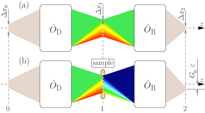
Figure 1: Graphical presentation of the echo spectroscopy principles. (a) Photons from a source with a linear size $\Delta x_{{}_{\mathrm{0}}}$ in the reference source plane $0$ are focused onto a spot $\Delta x_{{}_{\mathrm{1}}}$ in the intermediate image plane $1$ by a focusing-dispersing system $\hat{O}_{{}_{\mathrm{D}}}$. Each spectral component, indicated by different color, is focused at a different location due to dispersion in $\hat{O}_{{}_{\mathrm{D}}}$. All spectral components of the x-rays are refocused by a consecutive time-reversal focusing-dispersing system $\hat{O}_{{}_{\mathrm{R}}}$ onto the same spot $\Delta x_{{}_{\mathrm{2}}}$ (echo) in the image plane $2$. (b) Inelastic x-ray scattering with an energy transfer $\varepsilon$ (indicated by changed color) from a sample in the reference plane $1$ results in a lateral shift $G_{{}_{\mathrm{R}}}\varepsilon$ of the echo signal equal for all spectral components. Here $G_{{}_{\mathrm{R}}}$ is a linear dispersion rate in the time-reversal system $\hat{O}_{{}_{\mathrm{R}}}$. Spectral resolution of the x-ray echo spectrometer is $\Delta\varepsilon=\Delta x_{{}_{\mathrm{2}}}/G_{{}_{\mathrm{R}}}$.

Focusing of the monochromatic spectral components requires that matrix element $B=0$. The ray-transfer matrix of any focusing-dispersing system in a general case therefore reads as

$$\hat{O}=\{A\,0\,G;\,CDF;001\}$$ (1)

with $A$ and $G$ elements defined above. The system blurs the polychromatic source image, because of linear dispersion, as mentioned earlier and graphically presented in Fig. 1(a). However, another focusing-dispersing system can be used to refocus the source onto reference plane 2. Indeed, propagation of x-rays through the defocusing system $\hat{O}_{{}_{\mathrm{D}}}$ and a second system, which we will refer to as a refocusing or time-reversal system $\hat{O}_{{}_{\mathrm{R}}}$ (see Fig. 1) is given by a combined ray-transfer matrix

$$\hat{O}_{{}_{\mathrm{C}}}=\hat{O}_{{}_{\mathrm{R}}}\hat{O}_{{}_{\mathrm{D}}}=\{A_{{}_{\mathrm{C}}}\,0\,G_{{}_{\mathrm{C}}};C_{{}_{\mathrm{C}}}D_{{}_{\mathrm{C}}}F_{{}_{\mathrm{C}}};001\}\\ =\left(\!\!\begin{array}[]{ccc}A_{{}_{\mathrm{R}}}A_{{}_{\mathrm{D}}}&0&A_{{}_{\mathrm{R}}}G_{{}_{\mathrm{D}}}+G_{{}_{\mathrm{R}}}\\ C_{{}_{\mathrm{R}}}A_{{}_{\mathrm{D}}}\!+\!D_{{}_{\mathrm{R}}}C_{{}_{\mathrm{R}}}&D_{{}_{\mathrm{R}}}D_{{}_{\mathrm{D}}}&C_{{}_{\mathrm{R}}}G_{{}_{\mathrm{D}}}\!+\!D_{{}_{\mathrm{R}}}F_{{}_{\mathrm{D}}}\!+\!F_{{}_{\mathrm{R}}}\\ 0&0&1\end{array}\!\!\right),$$ (2)

and by a ray vector $\mbox{\boldmath$r$}_{{}_{2}}=(x_{{}_{2}},\xi_{{}_{2}},\delta E)=\hat{O}_{{}_{\mathrm{C}}}\mbox{\boldmath$r$}_{{}_{0}}$.

Here we arrive at a crucial point. If

$$G_{{}_{\mathrm{C}}}=A_{{}_{\mathrm{R}}}G_{{}_{\mathrm{D}}}+G_{{}_{\mathrm{R}}}=0,$$ (3)

the linear dispersion at the exit of the combined system vanishes, because dispersion in the defocusing system is compensated (time reversed) by dispersion in the refocusing system. As a result, the combined system refocuses all photons independent of the photon energy to the same location, $x_{{}_{2}}$ in image plane $2$, to a spot with a linear size

$$\Delta x_{{}_{2}}=|A_{{}_{\mathrm{R}}}A_{{}_{\mathrm{D}}}|\Delta x_{{}_{0}}\equiv|A_{{}_{\mathrm{R}}}|\Delta x_{{}_{1}},$$ (4)

as shown schematically in Fig. 1(a). Such behavior is an analog of the echo phenomena. Here, however, it takes place in space, rather than in the time domain.

Now, what happens if a sample is placed into the intermediate image plane $1$, [Fig. 1(b)], which can scatter photons inelastically? In an inelastic scattering process, a photon with an arbitrary energy $E+\delta E$, changes its value to $E+\delta E+\varepsilon$. Here $\varepsilon$ is an energy transfer in the inelastic scattering process. The ray vector $\mbox{\boldmath$r$}_{{}_{1}}=(x_{{}_{1}},\xi_{{}_{1}},\delta E)$ before scattering transforms to $\mbox{\boldmath$r$}_{{}_{1}}^{\prime}=(x_{{}_{1}},\xi_{{}_{1}}^{\prime},\delta E+\varepsilon)$ after inelastic scattering. Propagation of $\mbox{\boldmath$r$}_{{}_{1}}^{\prime}$ through the time-reversal system results in a ray vector $\mbox{\boldmath$r$}_{{}_{2}}^{\prime}=(x_{{}_{2}}^{\prime},\xi_{{}_{2}}^{\prime},\delta E+\varepsilon)=\hat{O}_{{}_{\mathrm{R}}}\mbox{\boldmath$r$}_{{}_{1}}^{\prime}$. Assuming that refocusing condition (3) holds, we come to a decisive point: all photons independent of the incident photon energy $E+\delta E$ are refocused to the same location

$$x_{{}_{2}}^{\prime}=x_{{}_{2}}+G_{{}_{\mathrm{R}}}\varepsilon,\hskip 14.22636ptx_{{}_{2}}=A_{{}_{\mathrm{R}}}A_{{}_{\mathrm{D}}}x_{{}_{o}},$$ (5)

which is, however, shifted from $x_{{}_{2}}$ by $G_{{}_{\mathrm{R}}}\varepsilon$, a value proportional to the energy transfer $\varepsilon$ in the inelastic scattering process. The essential point is that, the combined defocusing-refocusing system maps the inelastic scattering spectrum onto image plane $2$. The image is independent of the spectral composition $E+\delta E$ of the photons in the incident beam.

The spectral resolution $\Delta\varepsilon$ of the echo spectrometer is calculated from the condition, that the shift due to inelastic scattering $x_{{}_{2}}^{\prime}-x_{{}_{2}}=G_{{}_{\mathrm{R}}}\varepsilon$ is at least as large as the linear size $\Delta x_{{}_{2}}$ of the echo signal (4):

$$\Delta\varepsilon=\frac{\Delta x_{{}_{2}}}{|G_{{}_{\mathrm{R}}}|}\equiv\frac{|A_{{}_{\mathrm{R}}}|\Delta x_{{}_{1}}}{|G_{{}_{\mathrm{R}}}|}\equiv\frac{|A_{{}_{\mathrm{R}}}A_{{}_{\mathrm{D}}}|\Delta x_{{}_{o}}}{|G_{{}_{\mathrm{R}}}|}.$$ (6)

Here it is assumed that the spatial resolution of the detector is better than $\Delta x_{{}_{2}}$.

These results constitute the underlying principle of x-ray echo spectroscopy. Noteworthy, angular dispersion always results in an inclined intensity front, i.e., in dispersion both perpendicular to and along the beam propagation direction Shvyd’ko and Lindberg (2012). Therefore, x-rays are defocused and refocused also in the time domain, as in spin-echo. As a result, inelastic scattering spectra can be also mapped by measuring time distributions in the detector, given a short-pulse source.

Perfect refocusing takes place if the linear dispersion of the combined system $G_{{}_{\mathrm{C}}}=A_{{}_{\mathrm{R}}}G_{{}_{\mathrm{D}}}+G_{{}_{\mathrm{R}}}$ vanishes, as in Eq. (3). Refocusing can still take place with good accuracy if $|G_{{}_{\mathrm{C}}}|$ is sufficiently small:

$$|G_{{}_{\mathrm{C}}}|\Delta E_{\cup}\ll\Delta x_{{}_{2}}.$$ (7)

Here $\Delta E_{\cup}$ is the bandwidth of x-rays in image plane $2$. Tolerances on the echo spectrometer parameters and on the sample shape can be calculated with Eq. (7).

The above approach is general and applicable to any frequency domain. A particular version was proposed in the soft x-ray domain, for applications in resonant IXS spectroscopy at $L$-edges of $3d$ elements Fung et al. (2004); Lai et al. (2014). The dispersing elements in the soft x-ray and visible light domains are diffraction gratings. with diffraction gratings as dispersing elements Fung et al. (2004); Lai et al. (2014).

III Optical Design

Diffraction gratings are not practical in the hard x-ray regime. Extension into the hard x-ray regime is therefore nontrivial. In this regard, as was demonstrated in Shvyd’ko (2004); Shvyd’ko et al. (2006), the angular dispersion in the hard x-ray regime can be achieved by Bragg diffraction from asymmetrically cut crystals, i.e., from crystals with the reflecting atomic planes not parallel to the entrance surface. This is a hard x-ray analog of the optical diffraction gratings or optical prisms. A large dispersion rate is a key for achieving high spectral resolution in angular-dispersive x-ray spectrometers Shvyd’ko et al. (2014); Shvyd’ko (2015), including echo spectrometers, see Eq. (6). This is achieved, first, by using strongly asymmetric Bragg reflections close to backscattering Shvyd’ko (2004); Shvyd’ko et al. (2006), and, second, by enhancing the single-reflection dispersion rate considerably by subsequent asymmetric Bragg reflections from crystals in special arrangements Shvyd’ko et al. (2013) exemplified below. In the following two steps, we will show how the principle scheme of a generic echo spectrometer presented above, can be realized in the hard x-ray regime by using multi-crystal arrangements as dispersing elements.

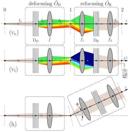
Figure 2: Principle optical scheme of an x-ray echo spectrometer, comprised of the defocusing $\hat{O}_{{}_{\mathrm{D}}}$ and refocusing $\hat{O}_{{}_{\mathrm{R}}}$ dispersing systems; the x-ray source in reference plane $0$; the sample in plane $1$; and the position-sensitive detector in $2$. The spectrometer is shown in the vertical dispersion plane for elastic (v${}_{{}_{\mathrm{e}}}$) and inelastic (v${}_{{}_{\mathrm{i}}}$) scattering, and in the horizontal scattering plane (h) with the refocusing system at a scattering angle $\Phi$. The defocusing system $\hat{O}_{{}_{\mathrm{D}}}$ consists of a dispersing Bragg diffracting (multi)crystal element D${}_{{}_{\mathrm{D}}}$, and of a focusing element $f$. The refocusing system $\hat{O}_{{}_{\mathrm{R}}}$ is of a spectrograph type comprising collimating element $f_{{}_{1}}$; a dispersing Bragg diffracting (multi)crystal element D${}_{{}_{\mathrm{R}}}$; and a focusing element $f_{{}_{2}}$.

In the first step, we propose a principle optical scheme of a hard x-ray echo spectrometer (Fig. 2) comprised of the defocusing $\hat{O}_{{}_{\mathrm{D}}}$ and refocusing $\hat{O}_{{}_{\mathrm{R}}}$ dispersing systems. The x-ray source is in reference plane $0$, the sample is in plane $1$, and the position-sensitive detector is in plane $2$. The defocusing system $\hat{O}_{{}_{\mathrm{D}}}$ is proposed here as a combination of a Bragg (multi)crystal dispersing element D${}_{{}_{\mathrm{D}}}$ and a focusing element $f$. As has been shown in Shvyd’ko (2015), such a system can be represented by a ray-transfer matrix (1) with the magnification $A_{{}_{\mathrm{D}}}$ and linear dispersion $G_{{}_{\mathrm{D}}}$ matrix elements given by

$$A_{{}_{\mathrm{D}}}\!=\!-\frac{1}{b_{\cup_{{}_{D}}}}\!\frac{l_{{}_{3}}}{l_{{}_{12}}},\hskip 5.69046ptG_{{}_{\mathrm{D}}}\!=\!{\mathcal{D}}_{\cup_{{}_{D}}}\frac{l_{{}_{3}}l_{{}_{1}}}{b_{\cup_{{}_{D}}}^{2}l_{{}_{12}}},\hskip 5.69046ptl_{{}_{12}}\!=\!\frac{l_{{}_{1}}}{b_{\cup_{{}_{D}}}^{2}}+l_{{}_{2}}.$$ (8)

Here, $l_{{}_{1}}$, $l_{{}_{2}}$, and $l_{{}_{3}}$, are the distances between the x-ray source, the dispersing element D${}_{{}_{\mathrm{D}}}$, the focusing element $f$ with focal length $f=(l_{{}_{12}}^{-1}+l_{{}_{3}}^{-1})^{-1}$, and the sample in the image plane $1$, respectively (Fig. 2). The dispersing (multi)crystal system D${}_{{}_{\mathrm{D}}}$ is characterized by the cumulative angular dispersion rate ${\mathcal{D}}_{\cup_{{}_{D}}}$, and cumulative asymmetry factor $b_{\cup_{{}_{D}}}$, which are defined in Shvyd’ko (2015) (see also Appendix A and Table 1).

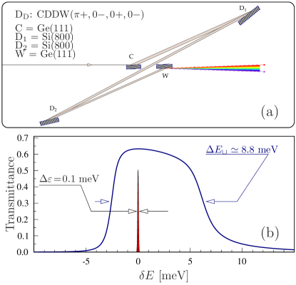
Figure 3: Dispersing element D${}_{{}_{\mathrm{D}}}$ (a) of the defocusing system $\hat{O}_{{}_{\mathrm{D}}}$ (see Fig. 2) and its spectral transmittance function (b). D${}_{{}_{\mathrm{D}}}$ is an example of an in-line four-crystal CDDW-type dispersing optic, comprised of collimating (C), dispersing (D${}_{{}_{1}}$, D${}_{{}_{2}}$), and wavelength-selecting (W) crystals in a ($\pi+$,$0-$,$0+$,$0-$) scattering configuration. With the crystal parameters provided in Table 2 of Appendix B, the dispersing element D${}_{{}_{\mathrm{D}}}$ features a spectral transmission function with a $\Delta E_{{}_{\cup}}=8.8$ meV bandwidth (b), a cumulative angular dispersion rate ${\mathcal{D}}_{\cup_{{}_{D}}}=-25~{}\mu$rad/meV, and a cumulative asymmetry factor $b_{\cup_{{}_{D}}}=1.4$. The sharp line in (b) presents the 0.1-meV spectral resolution of an x-ray echo spectrometer, designed for use with 9.1-keV photons.

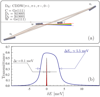
Figure 4: Dispersing element D${}_{{}_{\mathrm{R}}}$ (a) of the refocusing system $\hat{O}_{{}_{\mathrm{R}}}$ (see Fig. 2) and its spectral transmittance function (b). Similar to D${}_{{}_{\mathrm{D}}}$ in Fig. 3, D${}_{{}_{\mathrm{R}}}$ is an example of the in-line four-crystal CDDW-type dispersing optic, but, in a ($\pi+$,$\pi+$,$\pi-$,$0-$) scattering configuration. With the crystal parameters provided in Table 2 of Appendix B, the dispersing element D${}_{{}_{\mathrm{D}}}$ features a spectral transmission function with a $\Delta E_{{}_{\cup}}=5.5$ meV bandwidth (b), a cumulative angular dispersion rate ${\mathcal{D}}_{\cup_{{}_{D}}}=-43~{}\mu$rad/meV, a cumulative asymmetry factor $b_{\cup_{{}_{D}}}=0.36$, and ${\mathcal{D}}_{\cup_{{}_{D}}}/b_{\cup_{{}_{D}}}=-120~{}\mu$rad/meV.

For the spectrometer to feature a large throughput, the refocusing system $\hat{O}_{{}_{\mathrm{R}}}$ has to be capable of collecting x-ray photons in a large solid angle scattered from the sample. For this purpose, we propose using a hard x-ray focusing-dispersing system of a spectrograph-type considered in Shvyd’ko (2015), and schematically shown in Fig 2. A collimating focusing element $f_{{}_{1}}$ collects photons in a large solid angle and makes x-ray beams of each spectral component parallel. The collimated beams impinge upon the Bragg (multi)crystal dispersing element D${}_{{}_{\mathrm{R}}}$ with the cumulative angular dispersion rate ${\mathcal{D}}_{\cup_{{}_{R}}}$, and the cumulative asymmetry factor $b_{\cup_{{}_{R}}}$. The focusing element $f_{{}_{2}}$ focuses x-rays in the vertical dispersion plane onto the detector placed in the image plane $2$. As shown in Shvyd’ko (2015) (see also Appendix A and Table 1) such a system is described by a ray-transfer matrix (1) with the magnification $A_{{}_{\mathrm{R}}}$ and linear dispersion $G_{{}_{\mathrm{R}}}$ matrix elements given by

$$A_{{}_{\mathrm{R}}}=-\frac{b_{\cup_{{}_{R}}}f_{{}_{2}}\!}{f_{{}_{1}}\!},\hskip 14.22636ptG_{{}_{\mathrm{R}}}={\mathcal{D}}_{\cup_{{}_{R}}}f_{{}_{2}}.$$ (9)

Using Eqs. (3), (8), and (9) we obtain for the refocusing condition in the hard x-ray echo spectrometer

$$\frac{l_{{}_{3}}l_{{}_{1}}}{l_{{}_{1}}+b_{\cup_{{}_{D}}}^{2}l_{{}_{2}}}{\mathcal{D}}_{\cup_{{}_{D}}}=f_{{}_{1}}\frac{{\mathcal{D}}_{\cup_{{}_{R}}}}{b_{\cup_{{}_{R}}}}.$$ (10)

The dispersing element D${}_{{}_{\mathrm{D}}}$ can be placed from the source at a large distance $l_{{}_{1}}\gg b_{\cup_{{}_{D}}}^{2}l_{{}_{2}}$. In this case, the refocusing condition (10) reads

$$l_{{}_{3}}{\mathcal{D}}_{\cup_{{}_{D}}}\simeq f_{{}_{1}}\frac{{\mathcal{D}}_{\cup_{{}_{R}}}}{b_{\cup_{{}_{R}}}}.$$ (11)

For the spectral resolution $\Delta\varepsilon$ of a hard x-ray echo spectrometer we obtain from Eqs. (6), (8), and (9):

$$\Delta\varepsilon=\frac{|b_{\cup_{{}_{R}}}|}{|{\mathcal{D}}_{\cup_{{}_{R}}}|}\frac{\Delta x_{{}_{1}}}{f_{{}_{1}}}.$$ (12)

As follows from Eq. (12), the spectral resolution of the echo spectrometer is determined solely by the parameters of the refocusing system, i.e., by the resolution of the hard x-ray spectrograph Shvyd’ko (2015). The parameters of the defocusing system determine only the size of the secondary monochromatic source on the sample $\Delta x_{{}_{1}}=|A_{{}_{\mathrm{D}}}|\Delta x_{{}_{0}}$.

In the second step, we consider the particular optical designs of x-ray echo spectrometers with a very high spectral resolution $\Delta\varepsilon\lesssim 0.1$ meV. For practical reasons, we will assume that the secondary monochromatic source size is $\Delta x_{{}_{1}}\simeq 5~{}\mu$m, and the focal length is $f_{{}_{1}}\simeq 0.4$ m of the collimating element in the refocusing system. Then, Eq. (12) requires the ratio ${|{\mathcal{D}}_{\cup_{{}_{R}}}|}/{|b_{\cup_{{}_{R}}}|}\simeq 125~{}\mu$rad/meV for the dispersive element D${}_{{}_{\mathrm{R}}}$. Assuming the distance $l_{{}_{3}}\simeq 2$ m from the focusing element to the sample in the defocusing system, and $l_{{}_{1}}\gg b_{\cup_{{}_{D}}}^{2}l_{{}_{2}}$, we estimate from Eq. (10) for the required cumulative dispersing rate ${|{\mathcal{D}}_{\cup_{{}_{R}}}|}\simeq 25~{}\mu$rad/meV in the defocusing dispersive element. These are relatively large values. Typically, in a single Bragg reflection, a maximum dispersion rate is ${\mathcal{D}}\simeq 6-8~{}\mu$rad/meV for photons with energy $E\simeq 10$ keV Shvyd’ko et al. (2006, 2011). As mentioned before, multi-crystal arrangements can be used to enhance the dispersion rate Shvyd’ko et al. (2013).

Such large dispersion rates ${\mathcal{D}}_{\cup}$, unfortunately, tend to decrease the transmission bandwidths $\Delta E_{{}_{\cup}}$ of the dispersing elements Shvyd’ko et al. (2013); Shvyd’ko (2015). Achieving strong signals in IXS experiments, however, requires $\Delta E_{{}_{\cup}}\gg\Delta\varepsilon$. Therefore, optical designs of the dispersing elements have to be found featuring both large ${\mathcal{D}}_{\cup}$ and $\Delta E_{{}_{\cup}}$. Figures 3 and 4 show representative examples of multi-crystal CDDW-type inline dispersing elements Shvyd’ko et al. (2011); Stoupin et al. (2013); Shvyd’ko et al. (2014) of the defocusing and refocusing systems, respectively, with the required cumulative dispersion rates, asymmetry factors, and with bandwidths $\Delta E_{{}_{\cup}}\simeq 5.5-9$ meV, i.e., $\Delta E_{{}_{\cup}}/\Delta\varepsilon\simeq 55-90$, designed for use with 9.1-keV photons. These examples are modifications of the dispersing elements designs presented in Shvyd’ko (2015).

The CDDW optic in the ($\pi+$,$0-$,$0+$,$0-$) scattering configuration is preferred for the defocusing dispersing element D${}_{{}_{\mathrm{D}}}$ (Fig. 3) as it provides the required dispersion rate ${|{\mathcal{D}}_{\cup_{{}_{D}}}|}\simeq 25~{}\mu$rad/meV, significant transmission bandwidth $\Delta E_{{}_{\cup}}\simeq 9$ meV, and is compact. The CDDW optic in the ($\pi+$,$\pi+$,$\pi-$,$0-$) configuration is better suited for the refocusing dispersing element D${}_{{}_{\mathrm{R}}}$ (Fig. 4). It provides the large ratio ${|{\mathcal{D}}_{\cup_{{}_{R}}}|}/{|b_{\cup_{{}_{R}}}|}\simeq 120~{}\mu$rad/meV required for the high spectral resolution [see Eq. (12)] and substantial transmission bandwidth $\Delta E_{{}_{\cup}}\simeq 5.5$ meV, although smaller than in the D${}_{{}_{\mathrm{D}}}$-case.

The total beam size on the sample is $\simeq G_{{}_{\mathrm{D}}}\Delta E_{{}_{\cup}}$. For the spectrometer exemplified here, it is estimated to be $\simeq 275~{}\mu$m. Equation (7) together with Eqs. (8) and (9) can be used to estimate tolerances on the admissible variations of the focal distances, sample displacement, sample surface imperfections, etc. As discussed in Appendix D the tolerances are in a millimeter range in the case of the 0.1-meV spectrometer.

Details on the optical designs and examples of the dispersing elements designed for use with a lower photon energy of 4.57 keV and larger $\Delta E_{{}_{\cup}}\simeq 13-10$ meV, can be found in Appendix B. All these examples showcase the applicability of echo spectroscopy in a wide spectral range, and its feasibility both with synchrotron radiation and x-ray free electron laser sources.

The point is that even higher spectral resolution $\Delta\varepsilon\lesssim 0.02$ meV can be achieved with x-ray echo spectrometers by increasing the dispersion rates ${\mathcal{D}}_{\cup}$ in the dispersing elements. This, however, will result in their narrower transmission bandwidths $\Delta E_{{}_{\cup}}$. Still, an approximately constant ratio $\Delta E_{{}_{\cup}}/\Delta\varepsilon$ holds. Alternatively, the spectral resolution can be improved by increasing the focal length $f_{{}_{1}}$ in the refocusing system, see Eq. (12).

The essential feature of the echo spectrometers is that the signal strength, which is proportional to the product of the bandwidths of the photons on the sample and on the detector, is enhanced by $(\Delta E_{{}_{\cup}}/\Delta\varepsilon)^{2}\simeq 10^{3}-10^{4}$ compared to what is possible with the standard scanning-IXS-spectrometer approach.

IV Conclusions

In conclusion, x-ray echo spectroscopy, a counterpart of neutron spin-echo, is introduced here to overcome limitations in spectral resolution and weak signals of the traditional inelastic hard x-ray scattering (IXS) probes. Operational principles, refocusing conditions, and spectral resolutions of echo spectrometers are substantiated by an analytical ray-transfer-matrix approach. A principle optical scheme for a hard x-ray echo spectrometer is proposed with multi-crystal arrangements as dispersing elements. Concrete schemes are discussed with 5–13-meV transmission bandwidths, a spectral resolution of 0.1-meV (extension to 0.02-meV is realistic), and designed for use with 9.1-keV and 4.6-keV photons. The signal in echo spectrometers is enhanced by at least three orders of magnitude compared to what is possible with the standard scanning-IXS-spectrometer approach.

X-ray echo spectrometers require a combination of the CDDW dispersing elements and focusing optics as major optical components. Such components have been experimentally demonstrated recently Shvyd’ko et al. (2013, 2014). Implementation of x-ray echo spectrometers is, therefore, realistic.

V Acknowledgments

Stimulating discussions with D.-J. Huang (NSRRC) are greatly appreciated. S.P. Collins (DLS) is acknowledged for reading the manuscript and for valuable suggestions. Work at Argonne National Laboratory was supported by the U.S. Department of Energy, Office of Science, under Contract No. DE-AC02-06CH11357.

Appendix A Ray-transfer matrices

Ray-transfer matrices $\{A0G,CDF,001\}$ of the defocusing $\hat{O}_{{}_{\mathrm{D}}}$ and refocusing $\hat{O}_{{}_{\mathrm{R}}}$ systems of the x-ray echo spectrometers used in the paper are given in the last two rows of Table 1. They are equivalent to the derived in Ref. Shvyd’ko (2015) ray-transfer matrices of x-ray focusing monochromators and spectrographs. The matrices of the multi-element systems $\hat{O}_{{}_{\mathrm{D}}}$ and $\hat{O}_{{}_{\mathrm{R}}}$ are obtained by successive multiplication of the matrices of the constituent optical elements, which are given in the upper rows of Table 1.

In the first three rows, 1–3, matrices are shown for the basic optical elements, such as propagation in free space $\hat{P}(l)$, thin lens or focusing mirror $\hat{L}(f)$, and Bragg reflection from a crystal $\hat{C}(b,s{\mathcal{D}})$. Scattering geometries in Bragg diffraction from crystals are defined in Fig. 5. In the following rows of Table 1, ray-transfer matrices are shown for arrangements composed of several basic optical elements, such as successive multiple Bragg reflections from crystals $\hat{C}(b_{\cup_{{}_{n}}},{\mathcal{D}}_{\cup_{{}_{n}}})$ and $\hat{K}(b_{\cup_{{}_{n}}},{\mathcal{D}}_{\cup_{{}_{n}}},l)$, rows 4–5; and a focusing system $\hat{F}(l_{{}_{2}},f,l_{{}_{1}})$, row 6.

The matrices of the defocusing $\hat{O}_{{}_{\mathrm{D}}}$ and refocusing $\hat{O}_{{}_{\mathrm{R}}}$ systems presented in Table 1, rows 7 and 8, respectively, are calculated using the multi-crystal matrix $\hat{C}(b_{\cup_{{}_{n}}},{\mathcal{D}}_{\cup_{{}_{n}}})$ from row 4, assuming zero free space between crystals in successive Bragg reflections. Generalization to a more realistic case of nonzero distances between the crystals requires the application of matrix $\hat{K}(b_{\cup_{{}_{n}}},{\mathcal{D}}_{\cup_{{}_{n}}},l)$ from row 5.

We refer to Ref. Shvyd’ko (2015) for details on the derivation of these matrices. Here, we provide only the final results, notations, and definitions.

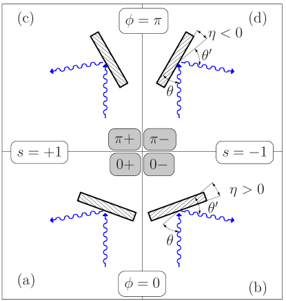
Figure 5: Definitions of scattering geometries in Bragg diffraction from a crystal: (a) $0+$, (b) $0-$, (c) $\pi+$, and (d) $\pi-$.

Optical system	Matrix notation	Ray-transfer matrix	Definitions and remarks
Free space Kogelnik and Li (1966); Hodgson and Weber (2005); Siegman (1986) (1)	$\hat{P}(l)$	$\left(\begin{array}[]{ccc}1&l&0\\ 0&1&0\\ 0&0&1\end{array}\right)$	$l$ – distance
Thin lens Kogelnik and Li (1966); Hodgson and Weber (2005); Siegman (1986) (2)	$\hat{L}(f)$	$\left(\begin{array}[]{ccc}1&0&0\\ -\frac{1}{f}&1&0\\ 0&0&1\end{array}\right)$	$f$ – focal length
Bragg reflection from a crystal Matsushita and Kaminaga (1980a, b) (3)	$\hat{C}(b,s{\mathcal{D}})$	$\left(\begin{array}[]{ccc}{1}/{b}&0&0\\ 0&b&s{\mathcal{D}}\\ 0&0&1\end{array}\right)$	$b=-\frac{\sin(\theta+\eta)}{\sin(\theta-\eta)}$ asymmetry factor; ${\mathcal{D}}=-(1/E)(1+b)\tan\theta$ angular dispersion rate.
Successive Bragg reflections Shvyd’ko (2015) $\hat{C}(\!b_{{}_{n}},s_{{}_{n}}{\mathcal{D}}_{{}_{n}}\!)\dotsb\hat{C}(\!b_{{}_{1}},s_{{}_{1}}{\mathcal{D}}_{{}_{1}}\!)$ (4)	$\hat{C}(b_{\cup_{{}_{n}}},{\mathcal{D}}_{\cup_{{}_{n}}})$	$\left(\begin{array}[]{ccc}1/b_{\cup_{{}_{n}}}&0&0\\ 0&b_{\cup_{{}_{n}}}&{\mathcal{D}}_{\cup_{{}_{n}}}\\ 0&0&1\end{array}\right)$	$b_{\cup_{{}_{n}}}=b_{{}_{1}}b_{{}_{2}}b_{{}_{3}}\dotsc b_{{}_{n}}$ ${\mathcal{D}}_{\cup_{{}_{n}}}=b_{{}_{n}}{\mathcal{D}}_{\cup_{{}_{n-1}}}+s_{{}_{n}}{\mathcal{D}}_{{}_{n}}$ $s_{i}=\pm 1$, $i=1,2,...,n$
Successive Bragg reflections with space between crystals Shvyd’ko (2015) $\hat{C}(\!b_{{}_{n}},s_{{}_{n}}{\mathcal{D}}_{{}_{n}}\!)\dotsb\hat{P}(\!l_{{}_{12}}\!)\hat{C}(\!b_{{}_{1}},s_{{}_{1}}{\mathcal{D}}_{{}_{1}}\!)$ (5)	$\hat{K}(b_{\cup_{{}_{n}}},{\mathcal{D}}_{\cup_{{}_{n}}},l)$	$\left(\begin{array}[]{ccc}1/b_{\cup_{{}_{n}}}&B_{\cup_{{}_{n}}}&G_{\cup_{{}_{n}}}\\ 0&b_{\cup_{{}_{n}}}&{\mathcal{D}}_{\cup_{{}_{n}}}\\ 0&0&1\end{array}\right)$	$B_{\cup_{{}_{n}}}\!=\!\frac{B_{\cup_{{}_{n-1}}}+b_{\cup_{{}_{n-1}}}l_{{}_{n-1n}}}{b_{{}_{n}}}$ $G_{\cup_{{}_{n}}}\!=\!\frac{G_{\cup_{{}_{n-1}}}+{\mathcal{D}}_{\cup_{{}_{n-1}}}l_{{}_{n-1n}}}{b_{{}_{n}}}$ $B_{\cup_{{}_{1}}}\!=\!0,\hskip 14.22636ptG_{\cup_{{}_{1}}}\!=\!0$
Focusing system $\hat{P}(l_{{}_{2}})\hat{L}(f)\hat{P}(l_{{}_{1}})$ (6)	$\hat{F}(l_{{}_{2}},f,l_{{}_{1}})$	$\left(\begin{array}[]{ccc}1-\frac{l_{{}_{2}}}{f}&B_{{}_{\mathrm{F}}}&0\\ -\frac{1}{f}&1-\frac{l_{{}_{1}}}{f}&0\\ 0&0&1\end{array}\right)$	$B_{{}_{\mathrm{F}}}=l_{{}_{1}}l_{{}_{2}}\left(\frac{1}{l_{{}_{1}}}+\frac{1}{l_{{}_{2}}}-\frac{1}{f}\right)$
Defocusing system $\hat{O}_{{}_{\mathrm{D}}}$ Shvyd’ko (2015) $\hat{F}(l_{{}_{3}},f,l_{{}_{2}})\hat{C}(b_{\cup_{{}_{n}}}\!,{\mathcal{D}}_{\cup_{{}_{n}}}\!)\hat{P}(l_{{}_{1}})$ (7)	$\hat{O}_{{}_{\mathrm{D}}}$	$\left(\!\!\begin{array}[]{ccc}\frac{1}{b_{\cup_{{}_{n}}}\!}\!\left(\!1\!-\!\frac{l_{{}_{3}}}{f}\!\right)&0&X{\mathcal{D}}_{\cup_{{}_{n}}}\\ -\frac{1}{fb_{\cup_{{}_{n}}}}&b_{\cup_{{}_{n}}}\!\!\left(\!1\!-\!\frac{l_{12}}{f}\!\right)&\left(\!1\!-\!\frac{l_{{}_{2}}}{f}\!\right)\!{\mathcal{D}}_{\cup_{{}_{n}}}\\ 0&0&1\end{array}\!\!\right)$	$\frac{1}{l_{{}_{12}}}\!+\!\frac{1}{l_{{}_{3}}}\!=\!\frac{1}{f}$ $l_{{}_{12}}=l_{{}_{1}}/b_{\cup_{{}_{n}}}^{2}+l_{{}_{2}}$ $X\!=\!l_{{}_{3}}l_{{}_{1}}\!/(\!b_{\cup_{{}_{n}}}^{2}\!l_{{}_{12}}\!)$
Refocusing system $\hat{O}_{{}_{\mathrm{R}}}$ Shvyd’ko (2015) $\hat{F}(\!f_{{}_{2}}\!,\!f_{{}_{2}}\!,\!l_{{}_{2}}\!)\hat{C}(\!b_{\cup_{{}_{n}}}\!,\!{\mathcal{D}}_{\cup_{{}_{n}}}\!)\hat{F}(\!l_{{}_{1}}\!,\!f_{{}_{1}}\!,\!f_{{}_{1}}\!)$ (8)	$\hat{O}_{{}_{\mathrm{R}}}$	$\left(\!\!\begin{array}[]{ccc}-\frac{b_{\cup_{{}_{n}}}f_{{}_{2}}\!}{f_{{}_{1}}\!}&0&f_{{}_{2}}{\mathcal{D}}_{\cup_{{}_{n}}}\\ \frac{(\!l_{{}_{1}}\!-\!f_{{}_{1}}\!)\!+\!(\!l_{{}_{2}}\!-\!f_{{}_{2}}\!)b_{\cup_{{}_{n}}}^{2}\!}{\!b_{\cup_{{}_{n}}}f_{{}_{1}}f_{{}_{2}}\!}&-\frac{f_{{}_{1}}}{b_{\cup_{{}_{n}}}\!f_{{}_{2}}}&\left(\!1\!-\!\frac{l_{{}_{2}}}{f_{{}_{2}}}\!\right)\!{\mathcal{D}}_{\cup_{{}_{n}}}\!\\ 0&0&1\end{array}\!\!\right)$

Table 1: Ray-transfer matrices $\{ABG,CDF,001\}$ of optical systems used in the paper. The matrices are shown starting with basic ones in rows 1–3. Matrices of combined systems are given in rows 4–6. The ray transfer matrices of the defocusing $\hat{O}_{{}_{\mathrm{D}}}$ and refocusing $\hat{O}_{{}_{\mathrm{R}}}$ systems of x-ray echo spectrometers are presented in rows 7–8. Definition of the glancing angle of incidence $\theta$ to the reflecting crystal atomic planes, the asymmetry angle $\eta$, and the deflection sign $s$ in Bragg diffraction from a crystal, used for the Bragg reflection ray-transfer matrix in row 3, are given in Fig. 5. See Ref. Shvyd’ko (2015) for more details.

Appendix B CDDW optic as dispersing element

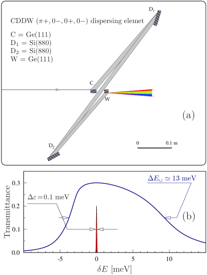
Figure 6: Dispersing element D${}_{{}_{\mathrm{D}}}$ (a) of the defocusing system $\hat{O}_{{}_{\mathrm{D}}}$ (Fig. 2) and its spectral transmittance function (b). D${}_{{}_{\mathrm{D}}}$ is an example of an in-line four-crystal CDDW-type dispersing optic, comprised of collimating (C), dispersing (D${}_{{}_{1}}$, D${}_{{}_{2}}$), and wavelength-selecting (W) crystals in a ($\pi+$,$0-$,$0+$,$0-$) scattering configuration. With the crystal parameters provided in Table 3, the dispersing element D${}_{{}_{\mathrm{D}}}$ features a spectral transmission function with a $\Delta E_{{}_{\cup}}=13$ meV bandwidth (b), a cumulative angular dispersion rate ${\mathcal{D}}_{\cup_{{}_{D}}}=-42~{}\mu$rad/meV, and a cumulative asymmetry factor $b_{\cup_{{}_{D}}}=1.4$. The sharp line in (b) presents the 0.1-meV design spectral resolution of the x-ray echo spectrometer. $E=4.5686$ keV.

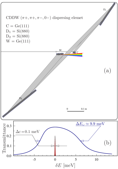
Figure 7: Dispersing element D${}_{{}_{\mathrm{R}}}$ (a) of the refocusing system $\hat{O}_{{}_{\mathrm{R}}}$ (Fig. 2) and its spectral transmittance function (b). Similar to D${}_{{}_{\mathrm{D}}}$ in Fig. 6, D${}_{{}_{\mathrm{R}}}$ is an example of the in-line four-crystal CDDW-type dispersing optic, but, in a ($\pi+$,$\pi+$,$\pi-$,$0-$) scattering configuration. With the crystal parameters provided in Table 3, the dispersing element D${}_{{}_{\mathrm{D}}}$ features a spectral transmission function with a $\Delta E_{{}_{\cup}}=9.9$ meV bandwidth (b), a cumulative angular dispersion rate ${\mathcal{D}}_{\cup_{{}_{D}}}=-64~{}\mu$rad/meV, a cumulative asymmetry factor $b_{\cup_{{}_{D}}}=0.39$, and ${\mathcal{D}}_{\cup_{{}_{D}}}/b_{\cup_{{}_{D}}}=-161~{}\mu$rad/meV. The sharp line in (b) presents the 0.1-meV design spectral resolution of the x-ray echo spectrometer. $E=4.5686$ keV.

In-line four-crystal CDDW-type dispersing optics Shvyd’ko et al. (2011); Stoupin et al. (2013); Shvyd’ko et al. (2014) are proposed in the paper for use as dispersing elements D${}_{{}_{\mathrm{D}}}$, D${}_{{}_{\mathrm{R}}}$ of the defocusing $\hat{O}_{{}_{\mathrm{D}}}$ and refocusing systems $\hat{O}_{{}_{\mathrm{R}}}$ of the echo spectrometer, respectively. The in-line four-crystal CDDW-type dispersing optic (see schematics in Figs. 3-4 and Figs. 6-7), comprises collimating (C), dispersing (D${}_{{}_{1}}$, D${}_{{}_{2}}$), and wavelength-selecting (W) crystals, which can be arranged in different scattering configurations. In a general case, the scattering configuration is defined as $(\phi_{{}_{1}}s_{{}_{1}},\phi_{{}_{2}}s_{{}_{2}},\phi_{{}_{3}}s_{{}_{3}},\phi_{{}_{4}}s_{{}_{4}})$. Here, for each crystal $n=1,2,3,4$ (1=C, 2=D${}_{{}_{1}}$, 3=D${}_{{}_{2}}$, 4=W) the value $\phi_{{}_{n}}=0$ corresponds to the grazing reflection, see Fig. 5(a)-(b); while $\phi_{{}_{n}}=\pi$ corresponds to the grazing incidence, see Fig. 5(c)-(d). The sign $s_{{}_{n}}=+1$ corresponds to a reflection in the counterclockwise direction, see Figs. 5(a),(c); while $s_{{}_{n}}=-1$ means the clockwise direction, see Figs. 5(b),(d). Those scattering geometries have been selected for use as dispersing elements of the x-ray echo spectrometer in the paper, which feature the largest cumulative dispersion rates ${\mathcal{D}}_{\cup_{{}_{n}}}$.

The cumulative dispersion rate ${\mathcal{D}}_{\cup_{{}_{4}}}$ in a four-crystal system is given in a general case by

$${\mathcal{D}}_{\cup_{{}_{4}}}=b_{{}_{4}}b_{{}_{3}}b_{{}_{2}}s_{{}_{1}}{\mathcal{D}}_{{}_{1}}+b_{{}_{4}}b_{{}_{3}}s_{{}_{2}}{\mathcal{D}}_{{}_{2}}+b_{{}_{4}}s_{{}_{3}}{\mathcal{D}}_{{}_{3}}+s_{{}_{4}}{\mathcal{D}}_{{}_{4}},$$ (13)

with the asymmetry parameters $b$ and dispersion rates ${\mathcal{D}}$ defined in Table 1, rows (3) and (4). For the CDDW-type dispersing elements considered in this paper the dispersion rate of the D-crystals ($n=2,3$) is much larger than those of the C- and W-crystals ($n=1,4$), see Tables 2 and 3. In this case, the cumulative dispersion rate can be approximated by ${\mathcal{D}}_{\cup_{{}_{4}}}\simeq b_{{}_{4}}b_{{}_{3}}s_{{}_{2}}{\mathcal{D}}_{{}_{2}}+b_{{}_{4}}s_{{}_{3}}{\mathcal{D}}_{{}_{3}}=b_{{}_{4}}(b_{{}_{3}}s_{{}_{2}}{\mathcal{D}}_{{}_{2}}+s_{{}_{3}}{\mathcal{D}}_{{}_{3}})$. The largest dispersion rates can be achieved in systems, in which the product is $s_{{}_{2}}s_{{}_{3}}{\mathcal{D}}_{{}_{2}}{\mathcal{D}}_{{}_{3}}<0$.

There are four high-dispersion-rate CDDW configurations featuring ${\mathcal{D}}_{{}_{2}}{\mathcal{D}}_{{}_{3}}>0$ and $s_{{}_{2}}s_{{}_{3}}<0$: $(\pi+,\pi-,\pi+,0+)$; $(\pi+,\pi+,\pi-,0-)$; $(\pi+,0-,0+,0-)$; and $(\pi+,0+,0-,0-)$. These configurations are especially interesting because of the incident and transmitted x-rays being parallel (in-line scheme).

There are four other high-dispersion-rate CDDW configurations featuring ${\mathcal{D}}_{{}_{2}}{\mathcal{D}}_{{}_{3}}<0$ and $s_{{}_{2}}s_{{}_{3}}>0$: $(\pi+,\pi-,0-,0-)$; $(\pi+,\pi+,0+,0-)$; $(\pi+,0-,\pi-,0-)$; and $(\pi+,0+,\pi+,0-)$. However, they are not in-line. The angle between the incident and reflected beams is $4(\theta_{\mathrm{D}}-\pi/2)$.

In the present paper, we have chosen the in-line high-dispersion-rate CDDW optic in the ($\pi+$,$0-$,$0+$,$0-$) configuration, as a dispersing element D${}_{{}_{\mathrm{D}}}$ of the defocusing system $\hat{O}_{{}_{\mathrm{D}}}$, see Figs. 3 and 6. The in-line high-dispersion-rate CDDW optic in the ($\pi+$,$\pi+$,$\pi-$,$0-$) configuration, was chosen as a dispersing element D${}_{{}_{\mathrm{R}}}$ of the refocusing system $\hat{O}_{{}_{\mathrm{R}}}$, see Figs. 4 and 7.

Tables 2 and 3 present crystal parameters and cumulative parameters of the dispersing elements designed for operations with x-rays with photon energies of 9.131385 keV and 4.5686 keV, respectively.

crystal	$\mbox{\boldmath$H$}_{{}_{\mathrm{e}}}$	$\eta_{{}_{\mathrm{e}}}$	$\theta_{{}_{\mathrm{e}}}$	$\Delta E_{{}_{\mathrm{e}}}$	$\Delta\theta_{{}_{\mathrm{e}}}$	$b_{{}_{\mathrm{e}}}$	$s_{{}_{\mathrm{e}}}{\mathcal{D}}_{{}_{\mathrm{e}}}$
element (e)
[material]	$(hkl)$	deg	deg	meV	$\mu$rad		$\frac{\mu{\mathrm{rad}}}{\mathrm{meV}}$
D${}_{{}_{\mathrm{D}}}$: CDDW ($\pi+$,$0-$,$0+$,$0-$), Fig. 3
1  C  [Ge]	(1 1 1)	-10.0	12.0	3013	71	-0.09	-0.02
2  D${}_{{}_{1}}$ [Si]	(8 0 0)	77.5	89	27	341	-1.17	-1.07
3  D${}_{{}_{2}}$ [Si]	(8 0 0)	77.5	89	27	341	-1.17	+1.07
4  W  [Ge]	(1 1 1)	10.0	12.0	3013	71	-10.8	-0.22
				$\Delta E_{{}_{\cup}}$	$\Delta\theta_{{}_{\cup}}^{\prime}$	$b_{\cup}$	${\mathcal{D}}_{\cup}$
				meV	$\mu$rad		$\frac{\mu{\mathrm{rad}}}{\mathrm{meV}}$
Cumulative values				8.8	-218	1.38	-25.0
D${}_{{}_{\mathrm{R}}}$: CDDW ($\pi+$,$\pi+$,$\pi-$,$0-$), Fig. 4
1  C  [Ge]	(1 1 1)	-10.0	12.0	3013	71	-0.09	-0.02
2  D${}_{{}_{1}}$ [Si]	(8 0 0)	-86	89	27	341	-0.6	-2.50
3  D${}_{{}_{2}}$ [Si]	(8 0 0)	-86	89	27	341	-0.6	+2.50
4  W  [Ge]	(1 1 1)	10.0	12.0	3013	71	-10.8	-0.22
Cumulative values				5.5	-237	0.36	-43.5

Table 2: Examples of the in-line four-crystal CDDW optics as dispersing elements (“diffraction gratings”) D${}_{{}_{\mathrm{D}}}$, D${}_{{}_{\mathrm{R}}}$ of the defocusing $\hat{O}_{{}_{\mathrm{D}}}$ and refocusing $\hat{O}_{{}_{\mathrm{R}}}$ systems of the echo spectrometer, respectively. For each optic, the table presents crystal elements (e=C,D${}_{{}_{1}}$,D${}_{{}_{2}}$,W) and their Bragg reflection parameters: $(hkl)$, Miller indices of the Bragg diffraction vector $\mbox{\boldmath$H$}_{{}_{\mathrm{e}}}$; $\eta_{{}_{\mathrm{e}}}$, asymmetry angle; $\theta_{{}_{\mathrm{e}}}$, glancing angle of incidence; $\Delta E_{{}_{\mathrm{e}}}^{({\mathrm{s}})}$, $\Delta\theta_{{}_{\mathrm{e}}}^{({\mathrm{s}})}$ are Bragg’s reflection intrinsic spectral width and angular acceptance in symmetric scattering geometry, respectively; $b_{{}_{\mathrm{e}}}$, asymmetry factor; and $s_{{}_{\mathrm{e}}}{\mathcal{D}}_{{}_{\mathrm{e}}}$, angular dispersion rate with deflection sign. For each optic, the table also shows the spectral window of imaging $\Delta E_{{}_{\cup}}$ as derived from the dynamical theory calculations, the angular spread of the dispersion fan $\Delta\theta_{{}_{\cup}}^{\prime}={\mathcal{D}}_{\cup}\Delta E_{{}_{\cup}}$, and the cumulative values of the asymmetry parameter $b_{\cup}$ and the dispersion rate ${\mathcal{D}}_{\cup}$. X-ray photon energy is $E=9.13185$ keV in both cases.

crystal	$\mbox{\boldmath$H$}_{{}_{\mathrm{e}}}$	$\eta_{{}_{\mathrm{e}}}$	$\theta_{{}_{\mathrm{e}}}$	$\Delta E_{{}_{\mathrm{e}}}$	$\Delta\theta_{{}_{\mathrm{e}}}$	$b_{{}_{\mathrm{e}}}$	$s_{{}_{\mathrm{e}}}{\mathcal{D}}_{{}_{\mathrm{e}}}$
element (e)
[material]	$(hkl)$	deg	deg	meV	$\mu$rad		$\frac{\mu{\mathrm{rad}}}{\mathrm{meV}}$
D${}_{{}_{\mathrm{D}}}$: CDDW ($\pi+$,$0-$,$0+$,$0-$), Fig. 6
1  C  [Ge]	(1 1 1)	-22.0	24.60	1542	154	-0.06	-0.09
2  D${}_{{}_{1}}$ [Si]	(4 0 0)	68	88	110	691	-1.19	-1.18
3  D${}_{{}_{2}}$ [Si]	(4 0 0)	68	88	110	691	-1.19	+1.18
4  W  [Ge]	(1 1 1)	22.0	24.55	1542	154	-16.4	-1.53
Cumulative values				13.0	-547	1.44	-41.9
D${}_{{}_{\mathrm{R}}}$: CDDW ($\pi+$,$\pi+$,$\pi-$,$0-$), Fig. 7
1  C  [Ge]	(1 1 1)	-22.0	24.60	1542	154	-0.06	-0.09
2  D${}_{{}_{1}}$ [Si]	(4 0 0)	-81.5	88	110	691	-0.62	-2.37
3  D${}_{{}_{2}}$ [Si]	(4 0 0)	-81.5	88	110	691	-0.62	+2.37
4  W  [Ge]	(1 1 1)	22.0	24.55	1542	154	-16.4	-1.53
Cumulative values				9.9	-638	0.39	-64.0

Table 3: Same as Table 2, however with the multi-crystal CDDW dispersing elements designed for an x-ray photon energy $E=4.5686$ keV.

Appendix C Focusing and collimating optics

Focusing and collimating optic elements are another key components of the x-ray echo spectrometers. There are no principal preferences of using either curved mirrors or compound-refractive lenses (CRL) for this purpose. However, in practical terms, mirrors maybe a preferable choise ensuring higher efficiency, because photoabsorption of 9.1-keV and especially of 4.5-keV photons is substantial in the CRLs Snigirev et al. (1996); Lengeler et al. (1999).

The focusing element $f$ in the defocusing dispersing system $\hat{O}_{{}_{\mathrm{D}}}$ (see Fig. 2) can be a standard K-B mirror system, ensuring a $\Delta x_{{}_{1}}\simeq 5~{}\mu$m vertical spot size in the echo-spectrometer example considered in the present paper. Tight focusing in the horizontal plane is also advantageous to minitage the negative effect on the spectral resolution of a ”projected” scattering source size with increasing scattering angle.

The collimating element $f_{{}_{1}}$ in the refocusing dispersing system $\hat{O}_{{}_{\mathrm{R}}}$ collects photons in a large solid angle $\Omega_{{}_{\mathrm{h}}}\times\Omega_{{}_{\mathrm{v}}}$, with $\Omega_{{}_{\mathrm{h}}}\simeq 10$ mrad, $\Omega_{{}_{\mathrm{h}}}\simeq 1-10$ mrad (depending on the required momentum transfer resolution, and makes the x-ray beam parallel. Laterally graded multilayer Montel mirrors recently proved to be useful exactly in this role Mundboth et al. (2014); Shvyd’ko et al. (2014).

The focusing element $f_{{}_{2}}$ in the refocusing dispersing system $\hat{O}_{{}_{\mathrm{R}}}$ focuses x-rays in the vertical dispersion plane onto the detector. Because the vertical beamsize after the dispersing element D${}_{{}_{\mathrm{R}}}$ is increased by $1/b_{\cup_{{}_{D}}}$ (an inverse of the cumulative asymmetry factor $b_{\cup_{{}_{D}}}$) the $f_{{}_{2}}$ element has to have a relatively large vertical geometrical aperture $\simeq 2-5$ mm (depending on the required spectral resolution). One-dimensional parabolic mirrors should be able to deal effectively with this problem.

Appendix D Echo spectrometer tolerances

Tolerances on the echo spectrometer parameters can be calculated from Eq. (7) in a general case. The equation can be rewritten as

$$|G_{{}_{\mathrm{D}}}+G_{{}_{\mathrm{R}}}/A_{{}_{\mathrm{R}}}|\Delta E_{\cup}\ll\Delta x_{{}_{1}}$$ (14)

using Eq. (3) and the relationship $\Delta x_{{}_{2}}=|A_{{}_{\mathrm{R}}}|\Delta x_{{}_{1}}$ from Eq. (4),

In a particular case of the echo spectrometer, which optical scheme is shown in Fig. 2, the tolerances on the spectrometer parameters can be calculated from equation

$$\left|{\mathcal{D}}_{\cup_{{}_{D}}}\frac{l_{{}_{3}}l_{{}_{1}}}{b_{\cup_{{}_{D}}}^{2}l_{{}_{12}}}-\frac{{\mathcal{D}}_{\cup_{{}_{R}}}f_{{}_{1}}\!}{b_{\cup_{{}_{R}}}\!}\right|\Delta E_{\cup}\ll\Delta x_{{}_{1}}$$ (15)

which is obtained by combining Eq. (15) and Eqs.(8)-(9). If the dispersing element D${}_{{}_{\mathrm{D}}}$ is placed from the source at a large distance $l_{{}_{1}}\gg b_{\cup_{{}_{D}}}^{2}l_{{}_{2}}$, in this case, the tolerance equation simplifies to

$$\left|{\mathcal{D}}_{\cup_{{}_{D}}}l_{{}_{3}}-\frac{{\mathcal{D}}_{\cup_{{}_{R}}}f_{{}_{1}}\!}{b_{\cup_{{}_{R}}}\!}\right|\Delta E_{\cup}\ll\Delta x_{{}_{1}}.$$ (16)

As an example, we assume that the spectrometer parameters are perfectly adjusted, except for the distance $l_{{}_{3}}$ from the focusing mirror to the secondary source (to the sample). The tolerance interval $\Delta l_{{}_{3}}$ in this case can be estimated using Eq. (16) as

$$\left|\Delta l_{{}_{3}}\right|\ll\frac{\Delta x_{{}_{1}}}{|{\mathcal{D}}_{\cup_{{}_{D}}}|\Delta E_{\cup}}.$$ (17)

If the distance $f_{{}_{1}}$ from the secondary source (sample) to the collimating mirror is not perfectly adjusted, the tolerance interval $\Delta f_{{}_{1}}$ can be estimated in this case as

$$\left|\Delta f_{{}_{1}}\right|\ll\frac{\Delta x_{{}_{1}}b_{\cup_{{}_{R}}}}{|{\mathcal{D}}_{\cup_{{}_{R}}}|\Delta E_{\cup}}.$$ (18)

With the parameters of the 0.1-meV-resolution echo spectrometer provided in the paper ($\Delta x_{{}_{1}}=5~{}\mu$m; $\Delta E_{\cup}=5.5$ meV; $|{\mathcal{D}}_{\cup_{{}_{D}}}|=25~{}\mu$rad/meV; $|b_{\cup_{{}_{R}}}/{\mathcal{D}}_{\cup_{{}_{R}}}|=125~{}\mu$rad/meV), these tolerance intervals are estimated to be $\left|\Delta l_{{}_{3}}\right|\ll 36$ mm, and $\left|\Delta f_{{}_{1}}\right|\ll 7$ mm, respectively. These numbers are not extremely demanding.

Since the variations of $l_{{}_{3}}$ and $f_{{}_{1}}$ could be related to sample position displacement and surface imperfections or to the sample being installed at some angle to the incident beam, the above estimated numbers also provide constraints on imperfections in the sample shape in this particular case.

Appendix E Tuning the refocusing condition up

In practice, the refocusing condition given by Eq. (10) can be exactly satisfied by tuning the distance $l_{{}_{3}}$, between the focusing element $f$ and the sample, see Fig. 2. Given that the source-to-sample distance $l=l_{{}_{1}}+l_{{}_{2}}+l_{{}_{3}}$, as well as the focal distance $f=l_{{}_{12}}l_{{}_{3}}/(l_{{}_{12}}+l_{{}_{3}})$ are fixed, the distances $l_{{}_{1}}$ and $l_{{}_{2}}$ also have to be corrected by the positioning of the dispersing system D${}_{{}_{\mathrm{D}}}$, appropriately. The distances $l_{{}_{1}}$ and $l_{{}_{2}}$ are defined from the above mentioned constraints, by solving the equations

$$l_{{}_{1}}+l_{{}_{2}} =l-l_{{}_{3}}$$ (19)

$$\frac{l_{{}_{1}}}{b_{\cup_{{}_{D}}}^{2}}+l_{{}_{2}} =\frac{fl_{{}_{3}}}{l_{{}_{3}}-f}.$$ (20)

Appendix F Spectral window of imaging

The spectral window of the imaging of the echo spectrometer is defined by the bandwidths and their relative shifts of the defocusing and refocusing systems. The shape of the window of imaging can be measured by measuring the elastically scattered signal and scanning one bandwidth against another. The window of imaging can be shifted by shifting one of the bandwidths against another.

References

• Hahn (1950) E. L. Hahn, Phys. Rev. 80, 580 (1950).
• Mezei (1980) F. Mezei, ed., Neutron Spin Echo., vol. 128 of Lecture Notes in Physics (Springer, Berlin, 1980).
• Röhlsberger (2014) R. Röhlsberger, Phys. Rev. Lett. 112, 117205 (2014).
• Fung et al. (2004) H. S. Fung, C. T. Chen, L. J. Huang, C. H. Chang, S. C. Chung, D. J. Wang, T. C. Tseng, and K. L. Tsang, AIP Conf. Proc. 705, 655 (2004).
• Lai et al. (2014) C. H. Lai, H. S. Fung, W. B. Wu, H. Y. Huang, H. W. Fu, S. W. Lin, S. W. Huang, C. C. Chiu, D. J. Wang, L. J. Huang, et al., Journal of Synchrotron Radiation 21, 325 (2014).
• Shvyd’ko (2004) Yu. Shvyd’ko, X-Ray Optics – High-Energy-Resolution Applications, vol. 98 of Optical Sciences (Springer, Berlin Heidelberg New York, 2004).
• Shvyd’ko et al. (2006) Yu. V. Shvyd’ko, M. Lerche, U. Kuetgens, H. D. Rüter, A. Alatas, and J. Zhao, Phys. Rev. Lett. 97, 235502 (2006).
• Shvyd’ko et al. (2013) Yu. Shvyd’ko, S. Stoupin, K. Mundboth, and J. Kim, Phys. Rev. A 87, 043835 (2013).
• Shvyd’ko (2015) Yu. Shvyd’ko, Phys. Rev. A 91, 053817 (2015).
• Kogelnik and Li (1966) H. Kogelnik and T. Li, Appl. Opt. 5, 1550 (1966).
• Matsushita and Kaminaga (1980a) T. Matsushita and U. Kaminaga, Journal of Applied Crystallography 13, 472 (1980a).
• Siegman (1986) A. E. Siegman, Lasers (University Science Books, Sausalito, California, 1986).
• Shvyd’ko and Lindberg (2012) Yu. Shvyd’ko and R. Lindberg, Phys. Rev. ST Accel. Beams 15, 100702 (2012).
• Shvyd’ko et al. (2014) Yu. Shvyd’ko, S. Stoupin, D. Shu, S. P. Collins, K. Mundboth, J. Sutter, and M. Tolkiehn, Nature Communications 5:4219 (2014).
• Shvyd’ko et al. (2011) Yu. Shvyd’ko, S. Stoupin, D. Shu, and R. Khachatryan, Phys. Rev. A 84, 053823 (2011).
• Stoupin et al. (2013) S. Stoupin, Yu. V. Shvyd’ko, D. Shu, V. D. Blank, S. A. Terentyev, S. N. Polyakov, M. S. Kuznetsov, I. Lemesh, K. Mundboth, S. P. Collins, et al., Opt. Express 21, 30932 (2013).
• Hodgson and Weber (2005) N. Hodgson and H. Weber, Laser Resonators and Beam Propagation: Fundamentals, Advanced Concepts and Applications, Optical Sciences (Springer, Berlin Heidelberg New York, 2005).
• Matsushita and Kaminaga (1980b) T. Matsushita and U. Kaminaga, Journal of Applied Crystallography 13, 465 (1980b).
• Snigirev et al. (1996) A. Snigirev, V. Kohn, I. Snigireva, and B. Lengeler, Nature 384, 49 (1996).
• Lengeler et al. (1999) B. Lengeler, C. Schroer, J. Tümmler, B. Benner, M. Richwin, A. Snigirev, I. Snigireva, and M. Drakopoulos, J. Synchrotron Radiation 6, 1153 (1999).
• Mundboth et al. (2014) K. Mundboth, J. Sutter, D. Laundy, S. Collins, S. Stoupin, and Yu. Shvyd’ko, J. Synchrotron Radiation 21, 16 (2014).