PHYSICAL PROPERTIES OF SPECTROSCOPICALLY-CONFIRMED GALAXIES AT $z\geq 6$. III. STELLAR POPULATIONS FROM SED MODELING WITH SECURE Ly$\alpha$ EMISSION AND REDSHIFTS

Abstract

We present a study of stellar populations in a sample of spectroscopically-confirmed Lyman-break galaxies (LBGs) and Ly$\alpha$ emitters (LAEs) at $5.7<z<7$. These galaxies have deep optical and infrared images from Subaru, $HST$, and $Spitzer$/IRAC. We focus on a subset of 27 galaxies with IRAC detections, and characterize their stellar populations utilizing galaxy synthesis models based on the multi-band data and secure redshifts. By incorporating nebular emission estimated from the observed Ly$\alpha$ flux, we are able to break the strong degeneracy of model spectra between young galaxies with prominent nebular emission and older galaxies with strong Balmer breaks. The results show that our galaxies cover a wide range of ages from several to a few hundred million years (Myr), and a wide range of stellar masses from $\sim$10⁸ to $\sim$10${}^{11}\,M_{\sun}$. These galaxies can be roughly divided into an ‘old’ subsample and a ‘young’ subsample. The ‘old’ subsample consists of galaxies older than 100 Myr, with stellar masses higher than $10^{9}\,M_{\sun}$. The galaxies in the ‘young’ subsample are younger than $\sim$30 Myr, with masses ranging between $\sim$10⁸ and $\sim$ $3\times 10^{9}\,M_{\sun}$. Both subsamples display a correlation between stellar mass and star-formation rate (SFR), but with very different normalizations. The average specific SFR (sSFR, derived from a smoothly rising star-formation history) of the ‘old’ subsample is 3–4 Gyr^-1, consistent with previous studies of ‘normal’ star-forming galaxies at $z\geq 6$. The average sSFR of the ‘young’ subsample is an order of magnitude higher, likely due to starburst activity. Our results also indicate little or no dust extinction in the majority of the galaxies, as already suggested by their steep rest-frame UV slopes. Finally, LAEs and LBGs with strong Ly$\alpha$ emission are indistinguishable in terms of age, stellar mass, and SFR.

1. INTRODUCTION

Star-forming galaxies at $z\geq 6$ are natural tools to study the early galaxy formation and explore the history of cosmic reionization. In recent years, with the advances of instrumentation on the Hubble Space Telescope ($HST$) and large ground-based telescopes, the number of galaxies found at $z\geq 6$ has increased dramatically. The majority of these galaxies were photometrically selected Lyman-break galaxies (LBGs) using the dropout technique (e.g., Oesch et al., 2010; Yan et al., 2012; Ellis et al., 2013; Willott et al., 2013; Bouwens et al., 2015; Laporte et al., 2015). Some of them, among the brightest in the optical and near-IR, have been spectroscopically confirmed with deep observations (e.g., Jiang et al., 2011; Curtis-Lake et al., 2012; Ono et al., 2012; Schenker et al., 2012; Finkelstein et al., 2013; Pentericci et al., 2014; Oesch et al., 2015; Watson et al., 2015). A complementary way to find $z\geq 6$ galaxies is the narrow-band (or Ly$\alpha$) technique. This technique has a high success rate of spectroscopic confirmation. More than 200 Ly$\alpha$ emitters (LAEs) at $z\geq 6$ have been spectroscopically identified (e.g., Shimasaku et al., 2006; Hu et al., 2010; Ouchi et al., 2010; Kashikawa et al., 2011; Henry et al., 2012), including several at $z\geq 7$ (e.g., Iye et al., 2006; Rhoads et al., 2012; Shibuya et al., 2012; Konno et al., 2014). Many properties of high-redshift LAEs can be used to probe cosmic reionization (e.g., Silva et al., 2013; Treu et al., 2013; Cai et al., 2014; Dijkstra, 2014; Jensen et al., 2014; Momose et al., 2014).

Meanwhile, the physical properties of $z\geq 6$ galaxies are also being investigated. At $z\geq 6$, the rest-frame UV/optical light moves to the IR range. Therefore, IR observations, including the $HST$ near-IR and Spitzer Space Telescope ($Spitzer$) mid-IR observations, are essential to measure the properties of these galaxies. While properties such as the rest-frame UV slope and galaxy morphology can be directly measured from optical and near-IR images (e.g., McLure et al., 2011; Dunlop et al., 2013; Bouwens et al., 2014; Curtis-Lake et al., 2015; Kawamata et al., 2015), detailed physical properties such as age and stellar mass have to come from SED modeling of stellar populations based on the combination of optical, near-IR, and mid-IR data (Conroy, 2013). The optical data and $HST$ near-IR data measure the slope of the rest-frame UV spectrum, and constrain the properties of young stellar populations. $Spitzer$ IRAC provides mid-IR photometry. When combined with $HST$ near-IR data, it measures the amplitude of the Balmer break and constrains the properties of older stellar populations. Soon after the launch of $Spitzer$, it was found that IRAC is sensitive enough to directly detect luminous $z\geq 6$ LBGs (e.g., Egami et al., 2005; Eyles et al., 2005; Yan et al., 2005). In these early results, $z\simeq 6$ LBGs showed strong IRAC detections, suggesting the existence of established massive stellar populations in their galaxies. Later studies then found that most galaxies were actually not detected in moderately deep IRAC images, meaning that they were considerably younger and less massive (e.g., Yan et al., 2006; Eyles et al., 2007; Pirzkal et al., 2007). Extensive studies are now being carried out with various galaxy samples, and a diversity of physical properties are found (e.g., González et al., 2010; Schaerer & de Barros, 2010; McLure et al., 2011; Labbé et al., 2013; Curtis-Lake et al., 2013; de Barros et al., 2014). These studies are mostly based on photometrically-selected samples, and their galaxies are not spectroscopically confirmed.

This paper is the third in a series presenting the physical properties of a large sample of spectroscopically confirmed galaxies at $z\geq 6$. In the first paper of the series (Jiang et al., 2013a, hereafter Paper I), we presented deep $HST$ and $Spitzer$ observations of 67 spectroscopically-confirmed galaxies at $z\geq 6$. The sample is the largest collection of spectroscopically confirmed galaxies in this redshift range, including 51 LAEs and 16 LBGs. We measured basic properties of the rest-frame UV continuum and Ly$\alpha$ emission in these galaxies. In the second paper of the series (Jiang et al., 2013b, hereafter Paper II), we carried out a structural and morphological study of these galaxies. In this third paper we will fit and model the SEDs of the galaxies, and derive physical parameters such as age, stellar mass, and dust extinction. This is particularly important for high-redshift LAEs. Some early observations (e.g., Malhotra & Rhoads, 2002; Pirzkal et al., 2007) found that $z\geq 4.5$ LAEs consist of young stellar populations with low stellar masses (compared to LBGs). However, this could be due to selection effects (e.g., Dayal & Ferrara, 2012). For LAEs at $z\geq 5.7$, we currently have very little knowledge of their stellar populations. This is because almost all the known LAEs were discovered by ground-based telescopes, and do not have sufficiently deep infrared observations. Our paper includes a large sample of LAEs. This allows us, for the first time, to systematically study stellar populations in $z>5.7$ LAEs.

As mentioned in Paper I, the spectroscopic redshifts of this sample have great advantages for measuring physical properties of high-redshift galaxies. Secure redshifts remove one critical free parameter in the SED modeling. A model spectrum of a bright $z\geq 6$ galaxy is usually derived from 4–5 broad-band photometric points, e.g., 1 optical band, 2 $HST$ bands, 1–2 $Spitzer$ IRAC bands. Given the limited degrees of freedom, a spectroscopic redshift will significantly improve SED modeling, especially when gaseous or nebular emission is considered. It has been clear that strong nebular emission widely exists in high-redshift galaxies. For example, Stark et al. (2013) found that H$\alpha$ contributes more than 30% of the IRAC 1 flux in $4<z<5$ galaxies. In the analysis of a large LBG sample at $3<z<6$, de Barros et al. (2014) estimated that about 60–70% of the LBGs show prominent nebular emission lines. At $z\geq 6$, strong nebular lines such as [O iii] $\lambda$5007, H$\beta$, and H$\alpha$ enter the IRAC 1 and 2 bands (3.6 and 4.5 $\mu$m), which significantly affects the measurements of stellar populations (e.g., Robertson et al., 2010; Schaerer & de Barros, 2010; Finlator et al., 2011; Stark et al., 2013; de Barros et al., 2014). Photometric redshifts with large uncertainties may place these nebular lines in the wrong filter bands during SED fitting. With spectroscopic redshifts, the predicted observed wavelengths of nebular lines are securely known.

The structure of the paper is as follows. In Section 2 we briefly review our galaxy sample and the available data. In Section 3 we perform SED modeling of the galaxies using evolutionary synthesis models. We then present the derived stellar populations of the galaxies in Section 4, and discuss the results in Section 5. We summarize the paper in Section 6. Throughout the paper we adopt a $\Lambda$-dominated flat cosmology with $H_{0}=70$ km s^-1 Mpc^-1, $\Omega_{m}=0.3$, and $\Omega_{\Lambda}=0.7$. All magnitudes are on the AB system (Oke & Gunn, 1983).

2. GALAXY SAMPLE AND DATA

Our galaxy sample consists of 67 spectroscopically confirmed galaxies at $z\geq 6$, including 62 galaxies in the Subaru Deep Field (SDF; Kashikawa et al., 2004) and 5 galaxies in the Subaru XMM-Newton Deep Survey field (SXDS; Furusawa et al., 2008). The SDF sample has 22 LAEs at $z\simeq 5.7$, 25 LAEs at $z\simeq 6.5$, one LAE at $z=6.96$, and 14 LBGs at $5.9\leq z\leq 6.5$. The SXDS sample contains 3 LAEs at $z\simeq 6.5$ and 2 LBGs at $z\simeq 6$. All the LAEs at $z\simeq 5.7$ and 6.5 have a relatively uniform magnitude limit of 26 mag in the narrow bands NB816 and NB921, and thus make a well-defined sample. The LBGs were selected with different criteria, and have rather inhomogeneous depth, so they are not a statistically complete sample. The details of our galaxy sample can be found in Section 2 of Paper I. In the next two subsections we will briefly describe the data used for this paper.

2.1. Optical and Near-IR Imaging Data

The optical imaging data for the two fields SDF and SXDS were obtained with Subaru Suprime-Cam (Kashikawa et al., 2004; Furusawa et al., 2008). They consists of images in a series of broad and narrow bands. In Paper I, we produced a set of stacked images in six broad bands ($BVRi^{\prime}z^{\prime}y$) and three narrow bands (NB816, NB921, and NB973), by including all available data in the archive. Our stacked images have great depth with excellent PSF FWHM of $0\farcs 6-0\farcs 7$. In particular, the total integration time of the SDF $z^{\prime}$ and $y$ band images is 29 hr and 24 hr, corresponding to a depth of 27.1 mag and 26.2 mag, respectively ($5\sigma$ detection in a $2\arcsec$ diameter aperture). For the galaxies at $z<6$, these two bands do not cover the Ly$\alpha$ emission line, so they provide two important photometric points for SED modeling.

We obtained near-IR imaging data for the SDF galaxies in three $HST$ GO programs (11149: PI E. Egami; 12329 and 12616: PI L. Jiang). The $HST$ observations were made with NICMOS and WFC3. The majority of the galaxies were observed with WFC3 in the F125W (hereafter $J_{125}$) and F160W (hereafter $H_{160}$) bands. The typical integration time was two $HST$ orbits (roughly 5400 sec) per band, leading to a depth of $\sim 27.4$ mag ($5\sigma$ detection) in $J_{125}$ and a depth of $\sim 27.1$ mag in $H_{160}$ (see also Windhorst et al., 2011). The remaining several SDF galaxies were observed with NICMOS in the F110W (hereafter $J_{110}$) and $H_{160}$ bands. The typical integration time was also two $HST$ orbits, and the depth in the two bands are $\sim 26.4$ mag and $\sim 26.1$ mag, respectively. The five SXDS galaxies were covered by the UKIDSS Ultra-Deep Survey (UDS). Their $HST$ WFC3 near-IR data were obtained from the Cosmic Assembly Near-infrared Deep Extragalactic Legacy Survey (CANDELS; Grogin et al., 2011; Koekemoer et al., 2011). The exposure depth of the CANDELS UDS data is 1900 sec in $J_{125}$ and 3300 sec in $H_{160}$, slightly shallower than our WFC3 data for the SDF. All the optical and near-IR photometry is listed in Table 1 of Paper I.

Our galaxies represent the most luminous galaxies at $z\geq 6$, in terms of Ly$\alpha$ luminosity (for LAEs) or UV continuum luminosity (for LBGs). They cover the brightest UV luminosity range of $M_{1500}<-19.5$ mag, so the majority of them were detected ($>5\sigma$) in the near-IR images. In Paper I and Paper II we have shown that these galaxies have steep UV continuum slopes $\beta$ with a median value of $\beta=-2.3$. They have moderately strong rest-frame Ly$\alpha$ equivalent width (EW) in the range $\sim$10 to $\sim$200 Å. Their star-formation rates (SFRs) are moderate from a few to a few tens solar masses per year. These galaxies also exhibit a wide range of rest-frame UV continuum morphology in the $HST$ images, from compact features to multiple component systems. In this paper we will measure stellar populations in these galaxies.

2.2. $Spitzer$ Mid-IR Imaging Data

Table 1Mid-IR Photometry of the Galaxies in Our Sample

No.	R.A. (J2000)	Decl. (J2000)	Redshift	IRAC 1	IRAC 2
2	13:23:54.601	+27:24:12.72	5.654	$>$26.85	$\ldots$
3	13:24:16.468	+27:19:07.65	5.665	25.09$\pm$0.21	25.39$\pm$0.33
4	13:24:32.885	+27:30:08.82	5.671	24.78$\pm$0.22	$\ldots$
5	13:24:11.887	+27:41:31.81	5.681	$>$26.64	$\ldots$
10	13:24:33.097	+27:29:38.58	5.696	$>$26.35	$\ldots$
15	13:24:23.705	+27:33:24.82	5.710	24.04$\pm$0.07	24.29$\pm$0.11
17	13:23:44.747	+27:24:26.81	5.716	$>$26.56	$\ldots$
20	13:24:40.527	+27:13:57.91	5.724	25.20$\pm$0.30	$\ldots$
21	13:24:30.633	+27:29:34.61	5.738	$>$26.16	$\ldots$
22	13:24:41.264	+27:26:49.09	5.743	$>$26.43	$\ldots$
23	13:24:18.450	+27:16:32.56	5.922	25.11$\pm$0.16	$\ldots$
24	13:25:19.463	+27:18:28.51	6.002	25.15$\pm$0.22	$\ldots$
25	13:24:26.559	+27:15:59.72	6.032	24.30$\pm$0.07	24.47$\pm$0.13
27	13:24:10.766	+27:19:03.95	6.040	25.70$\pm$0.30	$\ldots$
28	13:24:42.452	+27:24:23.35	6.042	25.59$\pm$0.39	$\ldots$
29	13:24:05.895	+27:18:37.72	6.049	$>$26.56	$\ldots$
30	13:24:00.301	+27:32:37.95	6.062	25.50$\pm$0.35	$\ldots$
31	13:23:45.632	+27:17:00.53	6.112	25.06$\pm$0.20	$\ldots$
33	13:24:20.628	+27:16:40.47	6.269	$>$26.62	$\ldots$
34	13:23:45.757	+27:32:51.30	6.315	23.82$\pm$0.09	$\ldots$
35	13:24:40.643	+27:36:06.94	6.332	23.23$\pm$0.05	23.74$\pm$0.11
36	13:23:45.937	+27:25:18.06	6.482	25.00$\pm$0.19	25.20$\pm$0.28
37	13:24:18.416	+27:33:44.97	6.508	$>$26.61	$\ldots$
39	13:23:43.190	+27:24:52.04	6.534	$>$26.43	$\ldots$
40	13:24:55.772	+27:40:15.31	6.534	$>$26.59	$\ldots$
43	13:23:53.054	+27:16:30.75	6.542	25.30$\pm$0.24	$\ldots$
44	13:24:15.678	+27:30:57.79	6.543	23.77$\pm$0.05	24.02$\pm$0.09
45	13:24:40.239	+27:25:53.11	6.544	$>$26.39	$\ldots$
46	13:23:52.680	+27:16:21.76	6.545	$>$26.38	$\ldots$
47	13:24:10.817	+27:19:28.08	6.547	23.70$\pm$0.05	23.74$\pm$0.09
48	13:23:48.922	+27:15:30.33	6.548	$>$26.35	$\ldots$
49	13:24:17.909	+27:17:45.94	6.548	25.33$\pm$0.24	$\ldots$
50	13:23:44.896	+27:31:44.90	6.550	24.56$\pm$0.16	$\ldots$
52	13:24:35.005	+27:39:57.43	6.554	$>$26.48	$\ldots$
54	13:24:08.313	+27:15:43.49	6.556	25.14$\pm$0.25	25.21$\pm$0.36
58	13:24:43.427	+27:26:32.62	6.583	25.44$\pm$0.26	24.72$\pm$0.23
61	13:25:22.291	+27:35:19.95	6.599	24.08$\pm$0.07	24.50$\pm$0.18
62	13:23:59.766	+27:24:55.75	6.964	24.84$\pm$0.16	25.17$\pm$0.21
63	02:18:00.899	-05:11:37.69	6.023	24.49$\pm$0.12	24.97$\pm$0.25
64	02:17:35.337	-05:10:32.50	6.116	24.90$\pm$0.11	$\ldots$
66	02:18:20.701	-05:11:09.89	6.575	25.90$\pm$0.32	$\ldots$
67	02:17:57.585	-05:08:44.72	6.595	23.72$\pm$0.04	24.25$\pm$0.08

Note. — The sequence numbers of the galaxies in Column 1 correspond to the numbers in Column 1 of Table 1 in Paper I.

Our $Spitzer$ IRAC imaging data for the SDF were obtained from two GO programs 40026 (PI: E. Egami) and 70094 (PI: L. Jiang). Program 40026 was carried out during the $Spitzer$ cryogenic phase, and the other one was carried out in the Warm Mission phase. The two programs imaged roughly 70% of the SDF to a depth of 3–7 hours. They covered all 62 SDF galaxies in our sample with IRAC channel 1 (3.6 $\mu$m), and 51 (out of 62) galaxies with IRAC channel 2 (4.5 $\mu$m). The IRAC data were reduced with the $Spitzer$ Science Center (SSC) pipeline MOPEX. The details of the $Spitzer$ observations and IRAC data reduction were described in Paper I. The final co-added images have a pixel size of $0\farcs 6$, roughly a half of the IRAC native pixel scale.

The IRAC images for the SXDS galaxies were obtained from the Spitzer Extended Deep Survey (SEDS; Ashby et al., 2013). SEDS is a very deep imaging survey in the IRAC 1 and 2 bands over five well-studied fields, including the UDS. With an integration time of 12 hr per pointing, SEDS reaches 26 mag in IRAC 1. The SEDS co-added images also have a pixel scale of $0\farcs 6$. The IRAC thumbnail images of all galaxies are shown in Figure 12 of Paper I.

The IRAC mid-IR photometry is complicated by source confusion. In deep IRAC images, faint galaxies are often blended with nearby neighbors, so reliable photometry usually requires proper deblending and removal of neighbors. We performed source deblending using iGALFIT (Ryan, 2011), an interactive tool to run GALFIT (Peng et al., 2002). For each galaxy in our sample, the basic procedure is as follows. We first modeled its bright neighbors with iGALFIT. The model neighbors were convolved with a PSF image, and were subtracted from the original image. The PSF image was constructed from a number of bright (but unsaturated) point sources. We then carried out aperture photometry for this galaxy on the residual image. We used a 3 pixel ($1\farcs 8$) aperture radius, and computed its background in an annulus from 5 to 10 pixels. Finally we applied an aperture correction (roughly 0.4 mag), which was measured from the PSF image. If a galaxy was isolated from any bright neighboring objects, we performed aperture photometry directly, without removing neighbors.

The results of the above IRAC photometry are shown in Table 1, where we list the magnitudes (or $2\sigma$ upper limits) and errors for 42 (out of 67) galaxies in our sample. We have discarded the galaxies that have less than two broad-band photometric points in the optical and near-IR (too few data points for SED modeling). These discarded galaxies are all very faint in terms of their rest-frame UV continuum emission. They were barely (or not) detected in the $HST$ $J_{125}$ (or $J_{110}$) band, the deepest band that we have. This virtually puts a magnitude limit on our sample: galaxies fainter than $J_{125}\sim 27.2$ mag were discarded. In Table 1, we have also discarded the galaxies that are heavily blended with (or completely covered by) much brighter neighbors in the IRAC images. In these cases, the IRAC photometry of the galaxies is not reliable. In Table 1, the sequence numbers of the galaxies in Column 1 correspond to the numbers in Column 1 of Table 1 in Paper I. Column 2 lists the redshifts. Columns 3 and 4 list the aperture photometry in IRAC 1 and 2 channels. If a galaxy is not detected in IRAC 1, a $2\sigma$ upper limit is given. We do not give upper limits for IRAC 2. Our IRAC 2 data are often significantly shallower than the IRAC 1 data, thus the inclusion of the IRAC 2 upper limits put no significant constraints on SED modeling.

3. SED MODELING

In this section we perform SED modeling using the GALEV evolutionary synthesis models (Kotulla et al., 2009). The GALEV models are similar to other evolutionary synthesis models such as BC03 (Bruzual & Charlot, 2003) and STARBURST99 (Leitherer et al., 1999). One distinct feature of GALEV is that it provides an option to include metallicity-dependent gaseous or nebular emission (both continuum and line emission). As we will see, nebular emission is critical for the SED modeling of our galaxies.

For high-redshift galaxies, the quality of the SED fitting is usually dominated by data quality rather than the quality of synthesis models (e.g. Pirzkal et al., 2012), i.e., it is limited by the number of available photometric data points and photometric uncertainties. The galaxies in our sample, like $z\geq 6$ galaxies in many other samples, have only 3–5 broad-band photometric points available, including 1–2 ground-based optical points, 2 $HST$ near-IR points, and 1–2 IRAC mid-IR points. In addition, these galaxies are faint, with relatively large photometric uncertainties particularly in the IRAC bands. Among 42 galaxies shown in Table 1, 27 galaxies were detected ($>3\sigma$) in our IRAC 1 images, and 13 galaxies were also detected in the IRAC 2 images. In order to account for the associated systematic uncertainties, we model our measurements under a broad range of assumptions, with the view that the true physical parameters of our galaxies lies somewhere within the range of possibilities that we consider.

3.1. Stellar Populations with and without Nebular Emission

Table 2Comparison between the SED-fitting Results from the NoEM Model and the GALEV-EM Model

No.	$M_{\ast}$ ($10^{8}M_{\sun}$)			Age (Myr)			$E(B-V)$			$\chi_{r}^{2}$
	NoEM	EM		NoEM	EM		NoEM	EM		NoEM	EM
3	$62.4_{-24.8}^{+32.0}$	$18.1_{-0.8}^{+0.9}$		$200_{-104}^{+132}$	$40_{-36}^{+152}$		$0.04_{-0.04}^{+0.04}$	$0.02_{-0.02}^{+0.06}$		1.4	1.5
4	$114.0_{-10.0}^{+11.0}$	$3.5_{-0.2}^{+0.2}$		$928_{-316}^{+68}$	$4_{-0}^{+8}$		$0.00_{-0.00}^{+0.04}$	$0.00_{-0.00}^{+0.04}$		23.6	18.8
15	$368.8_{-16.6}^{+35.6}$	$15.7_{-0.7}^{+0.7}$		$976_{-84}^{+20}$	$4_{-0}^{+8}$		$0.04_{-0.04}^{+0.04}$	$0.08_{-0.04}^{+0.04}$		4.3	2.7
20	$166.0_{-45.8}^{+63.2}$	$44.1_{-25.7}^{+77.4}$		$656_{-404}^{+340}$	$88_{-84}^{+420}$		$0.14_{-0.06}^{+0.06}$	$0.16_{-0.06}^{+0.06}$		0.2	0.2
23	$127.5_{-5.7}^{+12.3}$	$7.3_{-0.3}^{+0.3}$		$988_{-276}^{+8}$	$8_{-4}^{+76}$		$0.00_{-0.00}^{+0.04}$	$0.04_{-0.04}^{+0.04}$		1.8	1.2
24	$86.1_{-11.1}^{+12.8}$	$3.8_{-0.2}^{+0.2}$		$632_{-264}^{+364}$	$4_{-0}^{+16}$		$0.00_{-0.00}^{+0.04}$	$0.00_{-0.00}^{+0.06}$		2.4	0.8
25	$356.2_{-16.0}^{+34.4}$	$14.4_{-0.6}^{+0.7}$		$992_{-52}^{+4}$	$4_{-0}^{+8}$		$0.08_{-0.04}^{+0.04}$	$0.12_{-0.04}^{+0.04}$		17.1	13.3
27	$93.1_{-31.6}^{+35.4}$	$3.2_{-0.3}^{+0.3}$		$988_{-468}^{+8}$	$4_{-0}^{+40}$		$0.06_{-0.06}^{+0.06}$	$0.08_{-0.08}^{+0.08}$		3.4	2.4
28	$56.8_{-9.6}^{+41.9}$	$2.8_{-0.4}^{+0.3}$		$536_{-364}^{+460}$	$4_{-0}^{+616}$		$0.00_{-0.00}^{+0.08}$	$0.00_{-0.00}^{+0.08}$		0.4	$<$0.1
30	$86.9_{-21.0}^{+71.2}$	$3.0_{-1.8}^{+1.0}$		$992_{-448}^{+4}$	$4_{-0}^{+24}$		$0.02_{-0.02}^{+0.10}$	$0.04_{-0.04}^{+0.08}$		3.7	2.7
31	$275.6_{-93.5}^{+141.5}$	$8.3_{-5.0}^{+3.7}$		$984_{-384}^{+12}$	$4_{-0}^{+16}$		$0.16_{-0.08}^{+0.08}$	$0.16_{-0.08}^{+0.08}$		1.8	1.0
34	$852.2_{-38.4}^{+82.2}$	$41.0_{-1.8}^{+1.9}$		$992_{-136}^{+4}$	$8_{-4}^{+12}$		$0.14_{-0.04}^{+0.04}$	$0.16_{-0.04}^{+0.06}$		3.2	1.4
35	$3314.4_{-291.6}^{+319.8}$	$102.5_{-4.6}^{+4.8}$		$976_{-112}^{+20}$	$4_{-0}^{+8}$		$0.36_{-0.04}^{+0.04}$	$0.36_{-0.04}^{+0.04}$		68.3	25.0
36	$157.7_{-13.9}^{+15.2}$	$124.9_{-11.0}^{+12.1}$		$992_{-200}^{+4}$	$984_{-392}^{+12}$		$0.02_{-0.02}^{+0.06}$	$0.00_{-0.00}^{+0.06}$		3.5	2.9
43	$129.4_{-26.6}^{+41.2}$	$4.5_{-0.4}^{+0.4}$		$992_{-236}^{+4}$	$4_{-0}^{+12}$		$0.06_{-0.06}^{+0.08}$	$0.08_{-0.08}^{+0.06}$		6.9	3.8
44	$983.9_{-44.3}^{+94.9}$	$68.0_{-3.1}^{+3.2}$		$992_{-96}^{+4}$	$12_{-8}^{+12}$		$0.16_{-0.04}^{+0.04}$	$0.20_{-0.04}^{+0.04}$		10.0	2.3
47	$758.3_{-127.6}^{+153.4}$	$388.1_{-79.8}^{+123.5}$		$440_{-80}^{+60}$	$312_{-84}^{+96}$		$0.18_{-0.04}^{+0.04}$	$0.14_{-0.04}^{+0.04}$		7.1	6.6
49	$207.8_{-42.7}^{+121.6}$	$6.1_{-3.7}^{+0.6}$		$996_{-436}^{+0}$	$4_{-0}^{+992}$		$0.12_{-0.08}^{+0.08}$	$0.12_{-0.08}^{+0.08}$		0.4	0.1
50	$1223.8_{-251.7}^{+389.5}$	$30.6_{-6.3}^{+7.9}$		$996_{-324}^{+0}$	$4_{-0}^{+12}$		$0.36_{-0.06}^{+0.08}$	$0.34_{-0.06}^{+0.08}$		1.5	0.5
54	$144.7_{-29.8}^{+84.7}$	$112.4_{-14.5}^{+42.8}$		$992_{-268}^{+4}$	$972_{-412}^{+24}$		$0.02_{-0.02}^{+0.08}$	$0.00_{-0.00}^{+0.06}$		1.9	1.6
58	$183.4_{-56.5}^{+81.7}$	$178.8_{-43.2}^{+56.9}$		$480_{-216}^{+332}$	$884_{-380}^{+112}$		$0.12_{-0.06}^{+0.06}$	$0.06_{-0.06}^{+0.06}$		1.9	3.1
61	$875.4_{-77.0}^{+129.7}$	$29.2_{-1.3}^{+1.4}$		$984_{-116}^{+12}$	$4_{-0}^{+8}$		$0.20_{-0.04}^{+0.04}$	$0.22_{-0.04}^{+0.04}$		16.4	9.3
62	$194.5_{-47.0}^{+61.9}$	$163.2_{-45.0}^{+62.1}$		$756_{-248}^{+240}$	$656_{-256}^{+304}$		$0.04_{-0.04}^{+0.06}$	$0.04_{-0.04}^{+0.06}$		1.6	1.5
63	$201.7_{-9.1}^{+19.5}$	$7.0_{-0.3}^{+0.3}$		$988_{-148}^{+8}$	$4_{-0}^{+8}$		$0.00_{-0.00}^{+0.04}$	$0.02_{-0.02}^{+0.04}$		6.3	2.9
64	$167.1_{-14.7}^{+16.1}$	$5.0_{-0.2}^{+0.2}$		$992_{-200}^{+4}$	$4_{-0}^{+8}$		$0.00_{-0.00}^{+0.06}$	$0.00_{-0.00}^{+0.06}$		6.5	3.8
66	$113.5_{-53.9}^{+102.8}$	$23.0_{-15.0}^{+56.8}$		$920_{-636}^{+76}$	$96_{-92}^{+900}$		$0.10_{-0.10}^{+0.10}$	$0.12_{-0.10}^{+0.10}$		$<$0.1	$<$0.1
67	$774.8_{-68.2}^{+74.8}$	$27.1_{-1.2}^{+1.3}$		$976_{-108}^{+20}$	$4_{-0}^{+8}$		$0.10_{-0.04}^{+0.04}$	$0.12_{-0.04}^{+0.04}$		27.2	3.3

Note. — This table compares the SED-fitting results from the NoEM Model and from the GALEV-EM Model with rSFH. The minimum and maximum values of age are 4 and 1000 Myr. When an age is close to the two limits, its errors are not reliable because of the lack of dynamic range. In addition, the fitting results with very large or small $\chi_{r}^{2}$ ($\chi_{r}^{2}\gg 1$ or $\chi_{r}^{2}\ll 1$) are not reliable.

Given the limited number of available photometric data points, we use as few free parameters as possible in our SED fitting. Compared to photometric samples, the advantage of our sample are the spectroscopic redshifts that remove one critical free parameter. The other major parameters for SED fitting are metallicity, dust extinction (or reddening), stellar mass, age, and star formation history (SFH). We adopt a Salpeter initial mass function (IMF) with a mass range of 0.1–100 $M_{\sun}$. For metallicity, the GALEV models provide two options: chemically consistent treatment or fixed metallicity values. We choose to use the fixed metallicity values as other synthesis models do. There is a strong age-metallicity degeneracy at young ages (many of our galaxies are young), and our data are not sufficient enough to break this degeneracy. So we fix metallicity to be 0.2 $Z_{\sun}$, which was suggested by the simulations in Finlator et al. (e.g. 2011).

We use two representative SFHs, an exponentially declining SFH and a smoothly rising SFH. For the exponentially declining SFH $\sim{\rm exp}(-t/\tau)$, we fix the decline factor $\tau$ to be 200 million years (Myr) (to reduce the number of free parameters). The SFR of this SFH declines slowly at young ages (younger than $\sim 200$ Myr) and is not sensitive to $\tau$ for $\tau>200$ Myr. At high redshift, a more realistic SFH is probably a smoothly rising SFH (e.g. Finlator et al., 2007, 2011; Papovich et al., 2011). GALEV has not included any rising SFHs yet, so we incorporate the smoothly rising SFH (SFR as a function of age) of Finlator et al. (2011) into the GALEV models. Hereafter we denote the above exponentially declining SFH and smoothly rising SFH as ‘dSFH’ and ‘rSFH’, respectively. Our purpose of using two SFH models is to explore the possible ranges of physical parameters, rather than distinguishing one model from the other. We do not use more complex SFHs that usually introduce new free parameters. We do not consider the simple stellar population (SSP) or an instantaneous burst model. The SSP model is physically difficult to understand our $z\geq 6$ galaxies. These galaxies have strong Ly$\alpha$ emission, and presumably have strong nebular emission (we will discuss this later). But the nebular emission produced by the SSP drops rapidly in the first few Myr, as the instantaneous burst goes off.

From SED modeling, we mainly constrain three physical quantities, including dust reddening $E(B-V)$, stellar mass $M_{\ast}$, and age. We use the reddening law of Calzetti et al. (2000), and allow $E(B-V)$ to range between 0.00 and 0.50 in steps of 0.02. The age provided by the GALEV models starts from 4 Myr in steps of 4 Myr. We allow age to vary between 4 Myr and 1000 Myr, which approaches the age of the universe at $z\sim 6$. For $z\geq 6$ galaxies with the limited number of photometric points, age is usually poorly constrained due to various degeneracies among parameters. On the contrary, mass is the amplitude of a model spectrum, and is thus thought to be more easily constrained (e.g. Papovich et al., 2001; Shapley et al., 2005; Conroy, 2013; Mobasher et al., 2015). In reality, the mass estimate depends on the mass-to-light (M/L) ratio, which in turn depends strongly on the age of stellar populations. The measurement of the M/L ratios in most normal-SED galaxies can be accurate to a level of $\sim 0.3$ dex, if the uncertainty is dominated by systematics (Conroy, 2013). However, the M/L ratios can be very uncertain for certain types of galaxies, or galaxies in certain age ranges (see Conroy (2013) for a review).

The GALEV models provide options to include (or not) nebular line and continuum emission. We use both options for each individual model, and denote models with and without nebular/gaseous emission as ‘EM’ and ‘NoEM’ models, respectively. In the rest of the paper, we mostly discuss the 27 galaxies that were detected in the IRAC 1 band (galaxy parameters cannot be properly constrained for our galaxies without IRAC 1 detections). We fit the models to the SEDs of the galaxies and derive the above parameters by the minimum $\chi^{2}$ method. These results are shown in Table 2. The 1$\sigma$ uncertainties quoted in the table are estimated in a standard way, i.e., allowing all other parameters to vary until $\Delta\chi^{2}=1$. Figure 1 compares the distributions of stellar mass, age, and $E(B-V)$ in the 27 galaxies for different models and SFHs. The two columns of panels from left to right in Figure 1 correspond to the dSFH and the rSFH models, respectively. The grey filled histograms represent the EM models, and the black unfilled histograms represent the NoEM models.

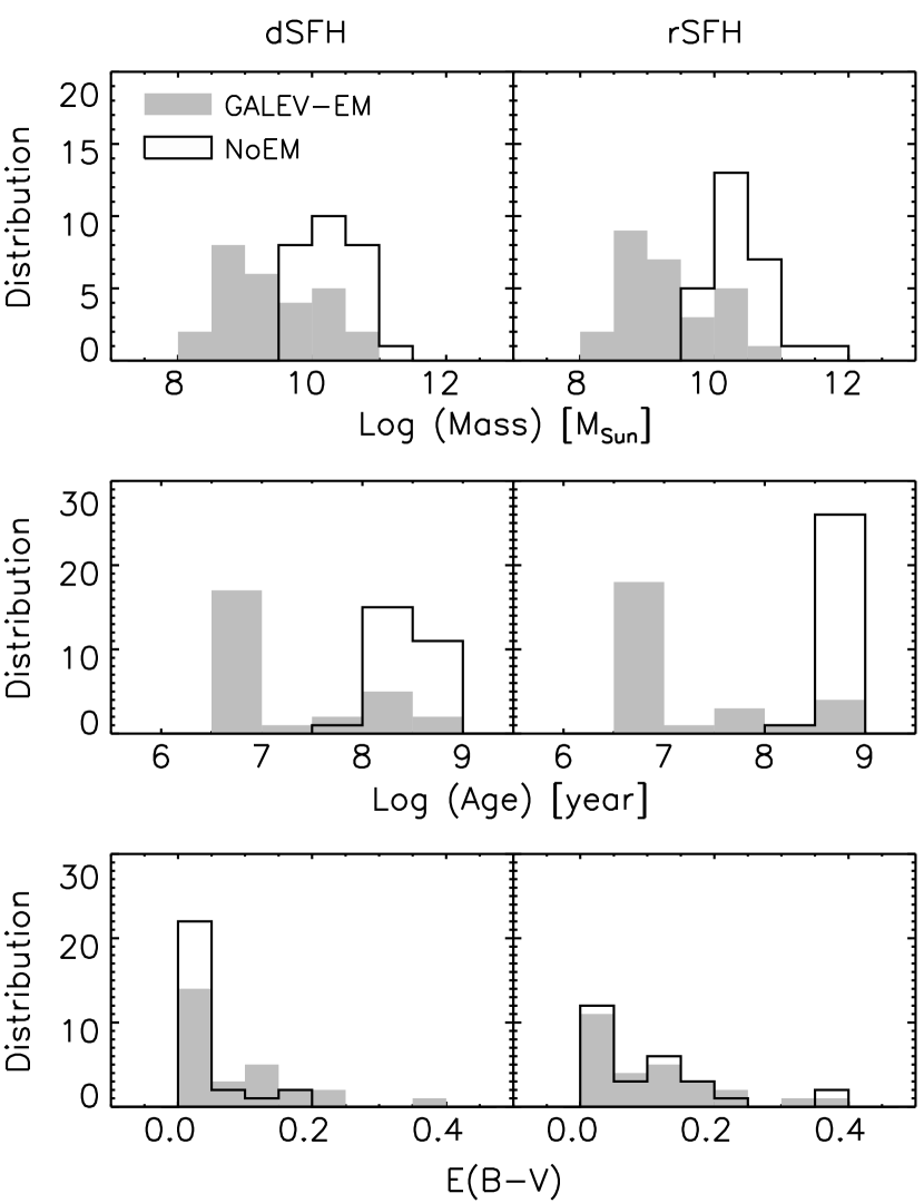
Figure 1.— Distributions of the stellar masses, ages, and $E(B-V)$ estimated for the 27 galaxies with the IRAC 1 detections. The two columns of the panels from the left to the right correspond to the declining SFH and the rising SFH, respectively. The grey filled histograms represent the EM models, and the black unfilled histograms represent the NoEM models. The NoEM and EM models produce different stellar populations (old and massive versus young and less massive) for the same galaxies. This is due to the strong degeneracy between young galaxies with prominent nebular emission and old galaxies with strong Balmer breaks.

Table 2 and Figure 1 show that the EM and NoEM models produce very different stellar populations for the same galaxies. Stellar populations of many galaxies from the EM models are very young, with ages of several Myr. They also have relatively low stellar masses. On the contrary, stellar populations from the NoEM models are mostly older than a few hundred Myr. They are usually very massive, with masses close to or higher than $10^{10}\,M_{\sun}$. Based on the minimum $\chi^{2}$ values, the quality of the EM models is comparable to (in some cases marginally better than) that of the NoEM models. The results are expected (e.g. Schaerer & de Barros, 2009), due to the the degeneracy between young galaxies with prominent nebular emission and old galaxies with strong Balmer breaks. This degeneracy is particularly strong for the galaxies in our sample for the following reasons. First, our galaxies are at $5.7<z<6.6$, so both IRAC 1 and 2 bands cover some of the strongest emission lines such as [O iii], H$\beta$, and H$\alpha$, etc. The second reason is that the IRAC 1 and 2 data have the largest photometric uncertainties compared to other bands; many galaxies were even not detected in the IRAC 2 band. Finally, for this redshift range, the wavelength range that IRAC 1 and 2 cover mimics the Balmer continuum/break that the synthesis models rely on to constrain stellar populations. The combination of these reasons make the EM and NoEM models indistinguishable for our galaxies.

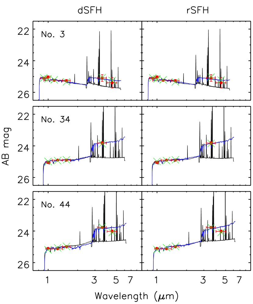
Figure 2.— Three examples of SED modeling illustrating the strong degeneracy between young galaxies with prominent nebular emission and older galaxies with strong Balmer breaks. The two columns of the panels correspond to the declining SFH and the rising SFH. The red points with error bars are the observed photometric data points. The horizontal errors indicate the wavelength ranges of the filters. The black and blue profiles represent the EM and NoEM models, respectively. The large green crosses represent the photometric points predicted by the EM models. The existence of emission lines in the EM models exactly mimics the the Balmer continua/breaks in the NoEM models, which significantly reduces the required ages and stellar masses of stellar populations in the EM models.

Figure 2 illustrates the degeneracy mentioned above by the SED modeling of three galaxies, one LAE at $z=5.664$ (No. 3), one LBG at $z=6.315$ (No. 34), and one LAE at $z=6.543$ (No. 44). The two columns of the panels from left to right correspond to the dSFH and the rSFH models, respectively. The red points with error bars are the observed photometric data points. The black and blue SED profiles represent the EM and NoEM models. Note that the GALEV models do not include the Ly$\alpha$ emission line. IGM absorption has been applied to the model spectra. We calculate the IGM absorption using the method of Fan et al. (2001) and Jiang et al. (2008). Note that the Ly$\alpha$ emission or the IGM absorption does not affect our SED fitting, because we did not use the bands that cover Ly$\alpha$. The figure shows that the existence of emission lines in the EM models mimics the Balmer continua/breaks in the NoEM models, which significantly reduces the age and stellar mass of stellar populations needed in the EM models.

3.2. Nebular Emission Estimated from the Ly$\alpha$ Line Emission

Table 3SED-fitting Results with the Ly$\alpha$-EM models

No.	$M_{\ast}$ ($10^{8}M_{\sun}$)			Age (Myr)			$E(B-V)$			$\chi_{r}^{2}$
	dSFH	rSFH		dSFH	rSFH		dSFH	rSFH		dSFH	rSFH
3	$7.2_{-0.3}^{+0.3}$	$7.2_{-0.3}^{+0.3}$		$4_{-0}^{+12}$	$4_{-0}^{+20}$		$0.04_{-0.04}^{+0.06}$	$0.04_{-0.04}^{+0.06}$		1.5	1.4
4	$3.4_{-0.1}^{+0.2}$	$3.4_{-0.1}^{+0.2}$		$4_{-0}^{+8}$	$4_{-0}^{+8}$		$0.00_{-0.00}^{+0.04}$	$0.00_{-0.00}^{+0.04}$		18.1	18.1
15	$127.3_{-11.2}^{+12.3}$	$21.1_{-0.9}^{+1.0}$		$168_{-24}^{+32}$	$8_{-4}^{+12}$		$0.00_{-0.00}^{+0.04}$	$0.08_{-0.04}^{+0.04}$		2.8	2.9
20	$29.5_{-9.1}^{+13.1}$	$32.8_{-10.1}^{+21.6}$		$148_{-128}^{+164}$	$492_{-468}^{+504}$		$0.02_{-0.02}^{+0.06}$	$0.02_{-0.02}^{+0.08}$		1.5	1.6
23	$46.8_{-6.0}^{+9.5}$	$57.9_{-9.8}^{+11.7}$		$124_{-48}^{+52}$	$444_{-208}^{+336}$		$0.00_{-0.00}^{+0.04}$	$0.00_{-0.00}^{+0.04}$		1.7	1.5
24	$3.8_{-0.2}^{+0.2}$	$3.8_{-0.2}^{+0.2}$		$4_{-0}^{+20}$	$4_{-0}^{+28}$		$0.00_{-0.00}^{+0.06}$	$0.00_{-0.00}^{+0.06}$		0.8	0.8
25	$20.9_{-0.9}^{+1.0}$	$66.5_{-5.8}^{+6.4}$		$12_{-8}^{+20}$	$956_{-184}^{+40}$		$0.10_{-0.04}^{+0.04}$	$0.02_{-0.02}^{+0.04}$		13.2	12.8
27	$12.6_{-1.6}^{+6.5}$	$17.4_{-4.2}^{+14.2}$		$88_{-84}^{+160}$	$324_{-320}^{+672}$		$0.00_{-0.00}^{+0.08}$	$0.00_{-0.00}^{+0.06}$		2.2	2.2
28	$2.7_{-0.2}^{+0.3}$	$2.7_{-0.2}^{+0.3}$		$4_{-0}^{+20}$	$4_{-0}^{+28}$		$0.00_{-0.00}^{+0.04}$	$0.00_{-0.00}^{+0.04}$		1.9	1.9
30	$43.4_{-8.9}^{+28.6}$	$26.8_{-4.5}^{+15.7}$		$192_{-136}^{+184}$	$912_{-728}^{+84}$		$0.00_{-0.00}^{+0.08}$	$0.00_{-0.00}^{+0.08}$		3.2	3.1
31	$2.4_{-1.7}^{+0.6}$	$2.4_{-2.2}^{+0.6}$		$4_{-0}^{+168}$	$4_{-0}^{+668}$		$0.04_{-0.04}^{+0.08}$	$0.04_{-0.04}^{+0.08}$		0.2	0.2
34	$640.7_{-107.8}^{+129.6}$	$250.0_{-11.2}^{+24.1}$		$356_{-44}^{+44}$	$992_{-204}^{+4}$		$0.06_{-0.04}^{+0.04}$	$0.12_{-0.04}^{+0.04}$		1.7	2.1
35	$54.2_{-2.4}^{+2.5}$	$81.1_{-3.7}^{+3.8}$		$592_{-8}^{+68}$	$4_{-0}^{+8}$		$0.00_{-0.00}^{+0.04}$	$0.34_{-0.06}^{+0.04}$		1.1	2.8
36	$109.8_{-18.5}^{+28.4}$	$46.4_{-4.1}^{+4.5}$		$240_{-60}^{+72}$	$988_{-236}^{+8}$		$0.00_{-0.00}^{+0.06}$	$0.00_{-0.00}^{+0.06}$		3.3	3.1
43	$76.3_{-15.7}^{+34.0}$	$30.8_{-7.4}^{+9.8}$		$284_{-120}^{+128}$	$972_{-528}^{+24}$		$0.00_{-0.00}^{+0.06}$	$0.02_{-0.02}^{+0.06}$		4.4	4.4
44	$331.1_{-29.1}^{+31.9}$	$172.9_{-15.2}^{+16.7}$		$260_{-32}^{+32}$	$872_{-160}^{+124}$		$0.06_{-0.04}^{+0.04}$	$0.08_{-0.04}^{+0.04}$		1.1	1.0
47	$368.7_{-16.6}^{+17.4}$	$391.1_{-107.8}^{+101.3}$		$76_{-20}^{+20}$	$184_{-40}^{+68}$		$0.18_{-0.04}^{+0.04}$	$0.18_{-0.04}^{+0.04}$		5.8	5.9
49	$59.3_{-21.9}^{+30.5}$	$35.6_{-16.9}^{+35.4}$		$196_{-148}^{+144}$	$212_{-208}^{+748}$		$0.04_{-0.04}^{+0.08}$	$0.08_{-0.08}^{+0.08}$		0.1	0.1
50	$173.5_{-97.8}^{+77.3}$	$9.0_{-1.9}^{+0.9}$		$528_{-72}^{+40}$	$4_{-0}^{+548}$		$0.06_{-0.06}^{+0.06}$	$0.22_{-0.08}^{+0.06}$		$<$0.1	$<$0.1
54	$36.5_{-6.2}^{+13.9}$	$51.5_{-10.6}^{+23.0}$		$112_{-84}^{+100}$	$460_{-392}^{+524}$		$0.00_{-0.00}^{+0.06}$	$0.00_{-0.00}^{+0.06}$		1.9	1.8
58	$138.7_{-33.5}^{+44.1}$	$61.6_{-14.9}^{+19.6}$		$268_{-76}^{+80}$	$960_{-384}^{+36}$		$0.02_{-0.02}^{+0.06}$	$0.04_{-0.04}^{+0.06}$		3.7	3.6
61	$357.6_{-31.5}^{+53.0}$	$66.3_{-3.0}^{+3.1}$		$516_{-24}^{+24}$	$32_{-28}^{+80}$		$0.00_{-0.00}^{+0.04}$	$0.20_{-0.04}^{+0.04}$		8.2	9.5
62	$128.0_{-21.5}^{+33.1}$	$115.0_{-31.7}^{+51.2}$		$228_{-64}^{+56}$	$472_{-216}^{+316}$		$0.00_{-0.00}^{+0.06}$	$0.04_{-0.04}^{+0.06}$		1.2	1.2
63	$9.8_{-0.4}^{+0.5}$	$9.4_{-0.4}^{+0.5}$		$8_{-4}^{+20}$	$8_{-4}^{+36}$		$0.02_{-0.02}^{+0.04}$	$0.02_{-0.02}^{+0.04}$		3.5	3.5
64	$35.2_{-3.1}^{+9.1}$	$41.3_{-11.4}^{+30.5}$		$72_{-44}^{+68}$	$200_{-136}^{+260}$		$0.00_{-0.00}^{+0.06}$	$0.00_{-0.00}^{+0.06}$		5.5	5.4
66	$1.4_{-0.8}^{+0.7}$	$1.4_{-1.2}^{+0.7}$		$4_{-0}^{+244}$	$4_{-0}^{+992}$		$0.00_{-0.00}^{+0.08}$	$0.00_{-0.00}^{+0.08}$		0.3	0.3
67	$32.0_{-1.4}^{+1.5}$	$32.0_{-1.4}^{+1.5}$		$4_{-0}^{+8}$	$4_{-0}^{+8}$		$0.14_{-0.04}^{+0.04}$	$0.14_{-0.04}^{+0.04}$		3.2	3.2

Note. — This table shows the SED-fitting results using the Ly$\alpha$-EM models, i.e., models with nebular emission estimated from the observed Ly$\alpha$ line flux (Section 3.2). The minimum and maximum values of age are 4 and 1000 Myr. When an age is close to the two limits, its errors are not reliable because of the lack of dynamic range.

With ongoing star formation in the models with rising and declining SFHs, nebular emission is naturally expected in our galaxies. In particular, we have seen strong Ly$\alpha$ emission lines in these galaxies. However, the actual strength of nebular emission, including continuum and line emission, is unknown. In the GALEV models that we use, the nebular emission is metallicity dependent, but its relative strength to the continuum is fixed in individual model galaxies. In other words, at any given age and metallicity for the same SFH, all galaxies have the same strength of nebular emission. This is a model assumption under certain physical conditions (electron temperature, atomic density, etc.). Real galaxies could have a wide range of nebular emission strength due to different physical states of the gas, including geometry.

In this subsection, we take a more realistic approach to estimate the strength of nebular emission using the observed Ly$\alpha$ line flux in our galaxy sample. One advantage of our sample, other than the available spectroscopic redshifts, is the known Ly$\alpha$ flux. Here we take advantage of this to estimate nebular emission, and incorporate the estimated nebular emission into our galaxy models. We first estimate the intrinsic Ly$\alpha$ flux for each galaxy based on the observed Ly$\alpha$ flux given in Paper I. Ly$\alpha$ emission is complicated and largely reduced by the resonant scattering of Ly$\alpha$ photons and the neutral IGM absorption. It is difficult to model Ly$\alpha$ radiative transfer and predict the intrinsic Ly$\alpha$ emission at high redshift. For a given apparent Ly$\alpha$ luminosity, its intrinsic luminosity could have a range of values. Zheng et al. (2010) showed that the distribution of the intrinsic to observed flux ratio ($f_{\rm Ly\alpha}^{\rm int}/f_{\rm Ly\alpha}^{\rm obs}$) peaks at $\sim$4 in relatively bright galaxies at $z\sim 5.7$. We thus assume $f_{\rm Ly\alpha}^{\rm int}/f_{\rm Ly\alpha}^{\rm obs}=4$ for our galaxies. As we already mentioned, the GALEV models do not include the Ly$\alpha$ emission line. We link the Ly$\alpha$ line flux to the model nebular line flux using H$\beta$ under Case B recombination, where the Ly$\alpha$ to H$\beta$ ratio ($f_{\rm Ly\alpha}^{\rm int}/f_{\rm H\beta}^{\rm int}$) is roughly 25 ($\rm Ly\alpha/H\alpha=8.7$ and $\rm H\alpha/H\beta=2.87$). The combination of the above two steps leads to an assumption that the ratio of the observed Ly$\alpha$ to the intrinsic H$\beta$ flux ratio ($f_{\rm Ly\alpha}^{\rm obs}/f_{\rm H\beta}^{\rm int}$) is 6.25, in the case of no dust extinction.

In order to incorporate this ratio to the GALEV models, we take each pair of the EM and NoEM model spectra in the whole parameter space from the previous subsection, and compute their nebular emission by subtracting the NoEM spectrum from the EM spectrum. We then scale the nebular emission (both line and continuum) to match the $f_{\rm Ly\alpha}^{\rm obs}/f_{\rm H\beta}^{\rm int}$ ratio (this ratio varies with dust extinction, and it is taken into account in this step). The details are as follows. We first take the Ly$\alpha$ EW from Paper I. Based on the continuum of the model spectrum, the Ly$\alpha$ EW, and the $f_{\rm Ly\alpha}^{\rm obs}/f_{\rm H\beta}^{\rm int}$ ratio, we calculate the H$\beta$ flux and EW for the model spectrum. Then the whole nebular emission spectrum is scaled and added to the model (continuum) spectrum. This model spectrum will have the required $f_{\rm Ly\alpha}^{\rm obs}/f_{\rm H\beta}^{\rm int}$ ratio during the SED fitting procedure. It does not guarantee that we will obtain the observed Ly$\alpha$ flux, because we only reserve its EW, the relative line flux to the continuum. Fortunately, there are no strong lines in the wavelength range covered by the non-IRAC data points (we did not use the bands that cover Ly$\alpha$). Therefore, the continuum at the wavelength of Ly$\alpha$ is well modeled (see Figures 2 and 3). It ensures that the Ly$\alpha$ flux in the best-fitting model spectrum is very close to the observed flux. This has been tested for each object, and it is accurate to a few percent.

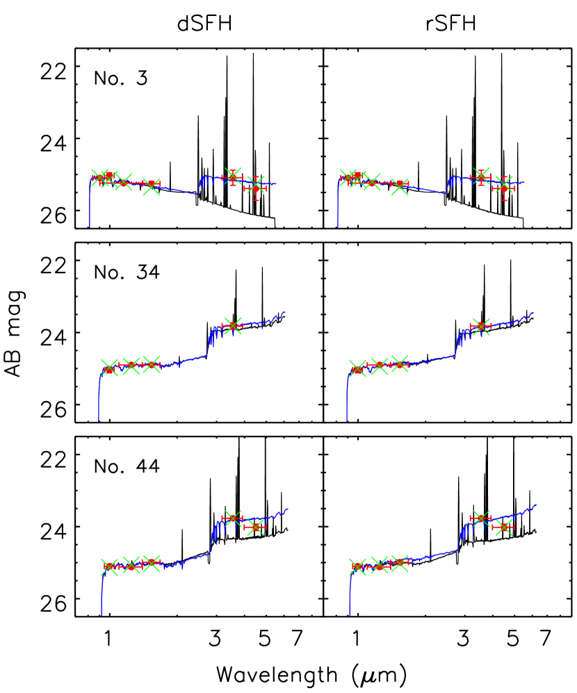
Figure 3.— Three examples of SED fitting with the Ly$\alpha$-EM models. The three galaxies are the same as shown in Figure 2. The red points with error bars are the observed photometric data points. The blue profiles are the NoEM model spectra shown as a reference (same as those in Figure 2). The Ly$\alpha$-EM model spectra are shown in black. The large green crosses represent the photometric points predicted by the EM models. The Ly$\alpha$-EM model spectra of No. 3 and No. 44 show strong nebular emission lines as seen in Figure 2. The spectra of No. 34 show much weaker lines compared to those in Figure 2, due to its weak Ly$\alpha$ emission line.

We next perform the SED modeling with the new EM models. We refer to these new EM models as ‘Ly$\alpha$-EM’ models, and the original GALEV EM models as ‘GALEV-EM’ models. Table 3 shows the results for the ‘Ly$\alpha$-EM’ models with dSFH and rSFH. Column 1 lists the galaxy sequence numbers. Columns 2–3 are stellar masses $M_{\ast}$ derived for the dSFH and the rSFH models, respectively. Columns 4–5 and Columns 6–7 are the derived ages and dust extinction for the two SFHs. Columns 8–9 give $\chi^{2}$ from the modeling. Figure 3 illustrates the new SED modeling of the three galaxies shown in Figure 2. The blue profiles are the NoEM model spectra shown as a reference. The Ly$\alpha$-EM model spectra are shown in black. The Ly$\alpha$-EM model spectra for objects No. 3 and No. 44 still show strong nebular emission lines, as seen in Figure 2. The spectra for object No. 34, however, have much weaker lines compared to those in Figure 2. This is due to its weak Ly$\alpha$ emission line (its rest-frame EW is only 8.6 Å). Figure 4 compares the distributions of stellar mass, age, and $E(B-V)$ for the Ly$\alpha$-EM and NoEM models. These distributions are roughly consistent with those for the GALEV-EM models shown in Figure 1. We will discuss this in detail in the next section.

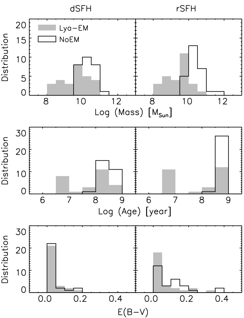
Figure 4.— Distributions of stellar mass, age, and $E(B-V)$ derived from the Ly$\alpha$-EM models. Like Figure 1, the grey filled histograms show the results from the Ly$\alpha$-EM models, and the black histograms show the results from the NoEM models as references.

4. RESULTS

For galaxies with strong nebular emission, the results of SED fitting strongly depend on the relative strength of nebular emission. In the above section, we used two methods to include nebular emission. One was to use the GALEV models with nebular emission (the GALEV-EM models), and the other one was to scale the nebular emission in the GALEV models to match our observed Ly$\alpha$ flux (the Ly$\alpha$-EM models). The latter one is a more realistic approach, and consists of two assumptions: the ratio of the observed to intrinsic Ly$\alpha$ flux $f_{\rm Ly\alpha}^{\rm int}/f_{\rm Ly\alpha}^{\rm obs}$ is 4, and the intrinsic Ly$\alpha$ to H$\beta$ flux ratio $f_{\rm Ly\alpha}^{\rm int}/f_{\rm H\beta}^{\rm int}$ is 25 (Case B), so that $f_{\rm Ly\alpha}^{\rm obs}/f_{\rm H\beta}^{\rm int}=6.25$. Each assumption involves non-negligible uncertainties. For the first assumption, the probability distribution function of $f_{\rm Ly\alpha}^{\rm int}/f_{\rm Ly\alpha}^{\rm obs}$ depends on the physical conditions of galaxies (Zheng et al., 2010). In addition, it is apparently a function of redshift: it increases (observed Ly$\alpha$ flux decreases) towards higher redshifts as the neutral fraction of the IGM increases. For the second assumption, real galaxies are more complex than the assumed ideal Case B recombination.

Despite the uncertainties mentioned above, our assumptions are reasonable (see more details in the discussion section). As we will see, the Ly$\alpha$-EM and GALEV-EM models produce roughly similar results on average, although there are large object-to-object variations due to the large range of the observed Ly$\alpha$ EW. In order to explore the possible ranges of physical parameters, we vary the $f_{\rm Ly\alpha}^{\rm obs}/f_{\rm H\beta}^{\rm int}$ ratio by a factor of two, i.e., we perform another two sets of SED modeling by assuming $f_{\rm Ly\alpha}^{\rm obs}/f_{\rm H\beta}^{\rm int}=3.125$ (referred to as EM-strong models), and $f_{\rm Ly\alpha}^{\rm obs}/f_{\rm H\beta}^{\rm int}=12.5$ (referred to as EM-weak models). Based on the simulations of Zheng et al. (2010), the majority of galaxies are included in the range considered here. We will discuss nebular emission and our assumptions in greater details in section 5.

4.1. Stellar Mass

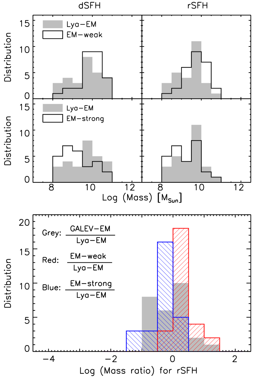
Figure 5.— Stellar masses derived from models with different nebular emission. In the upper four panels, the filled grey histograms show the stellar mass distributions from the Ly$\alpha$-EM models. The black unfilled histograms represent the distributions from the EM-weak models and the EM-strong models, which do not significantly deviate from those from the Ly$\alpha$-EM models. The bottom panel shows the distributions of the mass ratios for rSFH. The mass ratios of the GALEV-EM to Ly$\alpha$-EM models span a wide range due to the wide distribution of the Ly$\alpha$ EWs in our sample. The median value is close to 1. Models with stronger (weaker) nebular emission generally produce stellar populations with lower (higher) masses. On the other hand, the results for most galaxies from three EM models (Ly$\alpha$-EM, EM-weak, and EM-strong) are roughly consistent. About 70–80% galaxies in our sample have similar stellar masses (within a factor of 3) from the three different EM models.

It is worth briefly discussing the bias of our sample before we discuss the resulting stellar masses. The bias from sample selection was discussed in Paper I, and in Section 2 of this paper. The 42 galaxies in Table 1 are brighter than $\sim 27.2$ AB mag in $J$. The 27 galaxies shown in Figures 1 and 4 have detections in the IRAC 1 band (see also Table 1), so they are further limited by the 3.6 $\mu$m flux detection limit. Because the 3.6 $\mu$m flux is closely related to stellar mass for $z\sim 6$ galaxies, the sample of the 27 galaxies is biased towards the more massive galaxies. This is the reason that the stellar masses derived from the NoEM models are mostly close to or higher than $10^{10}\,M_{\sun}$ (see the histograms in Figures 1 and 4).

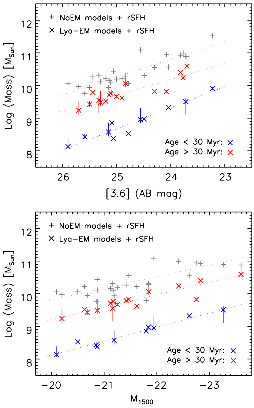
Figure 6.— Relations between stellar mass and brightness. The grey pluses represent the galaxies in the NoEM models with rSFH. For the EM models with rSFH, the galaxies are divided into two subsamples, a ‘young’ subsample (age $<$ 30 Myr; blue crosses) and an ‘old’ subsample (age $>$ 30 Myr; red crosses). The dotted lines are the best linear (in the log space) fits to the data points. Upper panel: stellar mass as a function of apparent magnitude at 3.6 $\mu$m. The masses derived from the NoEM models have a good correlation with the 3.6 $\mu$m magnitude, because stellar mass is the amplitude of a model spectrum. For the EM models, the relation is also tight in either subsample, due to the reasons explained in section 4.1. But many galaxies are significantly below the relation from the NoEM models, because of the presence of strong nebular emission in the IRAC 1 band. Lower panel: stellar mass as a function of absolute magnitude $M_{1500}$ at rest-frame 1500 Å. For the NoEM models, there is a weak correlation in which stellar masses are higher in more UV luminous galaxies. This correlation is more obvious in the two subsamples for the EM models. The correlation may reflect the mass-SFR relation seen at lower redshifts.

Stellar mass is thought to be the parameter that is least sensitive to model assumptions, because it is directly measured from the scaling of galaxy model spectra (e.g. Papovich et al., 2001; Shapley et al., 2005). When nebular emission is included, however, the measurement of stellar mass becomes less straightforward. Figure 5 compares the stellar masses derived from models with different nebular emission. The filled grey histograms show the stellar mass distributions from the Ly$\alpha$-EM models. The black unfilled histograms represent the mass distributions from the EM-weak models (top two panels) and the EM-strong models (middle two panels). The distributions of the EM-weak and EM-strong models do not significantly deviate from those for the Ly$\alpha$-EM models. The bottom panel shows the ratios of the stellar masses derived from different EM models. Although the mass ratios of the GALEV-EM to Ly$\alpha$-EM models span a wide range due to the wide distribution of the Ly$\alpha$ EW in our sample, the median ratio is close to 1, suggesting that the assumptions we made for the Ly$\alpha$-EM models are reasonable. We use the EM-weak and EM-strong models to explore the possible mass ranges. As expected, they show that models with stronger (weaker) nebular emission generally produce stellar populations with lower (higher) masses and younger (older) ages. On the other hand, the results for most galaxies from the three EM models (Ly$\alpha$-EM, EM-weak, and EM-strong) are roughly consistent. The bottom panel shows that about 70–80% galaxies in our sample have similar stellar masses (within a factor of 3) from the three different EM models.

The upper panel of Figure 6 shows the relation between the 3.6 $\mu$m flux and stellar mass derived from models with rSFH. There is a tight relation for the NoEM models (grey pluses), as explained above. For the EM models (the Ly$\alpha$-EM models here; crosses), the correlation still exists for the whole sample, but with a much larger scatter. The relation also significantly deviates from the relation for the NoEM models, due to the contamination of strong nebular emission in the IRAC 1 band. We divide these galaxies into two subsamples: a ‘young’ subsample (age $<$ 30 Myr; blue crosses) and an ‘old’ subsample (age $>$ 30 Myr; red crosses) based on the age distributions shown in Figures 4 and 8. The old subsample consists of galaxies with ages of several hundred Myr, and the galaxies in the young subsample are usually younger than 30 Myr (see subsection 4.2). It is obvious that the relation between the 3.6 $\mu$m flux and stellar mass is tight in either subsample. The linear Pearson correlation coefficients for the old and young subsamples are –0.87 and –0.96, respectively. The upper panel of Figure 7 shows the relation for dSFH, which is also obvious though less tight. The linear Pearson correlation coefficients for the two subsamples are –0.66 and –0.92, respectively. This relation is partially shaped by selection effects, i.e., these objects were selected in a relatively small parameter space. It may also be partially due to the following reasons. For the old subsample, the 3.6 $\mu$m flux is still dominated by stellar emission, and thus reflects the stellar mass. In the young subsample, nebular emission has a large contribution to the 3.6 $\mu$m flux. On the other hand, these galaxies are within a small range of (very young) age, and their relative strength of the nebular to stellar emission does not span a wide range (note that it is fixed for any GALEV-EM model SED). So the combination of the nebular and stellar emission still follow the correlation, though the presence of nebular emission has largely reduced the required stellar masses.

The lower panel in Figure 6 shows the relation between stellar mass and rest-frame UV luminosity $M_{1500}$, the absolute AB mag at 1500 Å derived in Paper I). The $M_{1500}$ values have been corrected for dust extinction. As for the upper panel, the pluses and crosses represent the NoEM and EM models, and the red and blue crosses represent the old and young subsamples, respectively. For the NoEM models, there is a weak correlation in which stellar masses are higher in more luminous galaxies. Such correlation is more tight in the two subsamples in the Ly$\alpha$-EM models. The linear Pearson correlation coefficients for the old and young subsamples are –0.92 and –0.99, respectively. The lower panel of Figure 7 shows the relation for dSFH, which is also obvious though less tight. The linear Pearson correlation coefficients for the two subsamples are –0.67 and –0.96, respectively. This relation has been reported in previous studies of high-redshift galaxies with different SFHs, including constant SFH and slowly varying (rising or declining) SFHs (e.g. Stark et al., 2009; González et al., 2011; McLure et al., 2011; Curtis-Lake et al., 2013). It is believed to be the high-redshift version of the mass-SFR relation (or the ‘so-called’ main sequence of star-forming galaxies) found at lower redshifts, in which the SFR is higher in more massive galaxies, and the normalization of the relation at higher redshift is higher (e.g. Daddi et al., 2007; Elbaz et al., 2007; Noeske et al., 2007). Objects with extreme star-forming activity may significantly deviate from the relation. In our sample the UV luminosity $M_{1500}$ reflects SFR. We will discuss the SFRs of our sample in section 4.4. The tight relations seen in the figure could also be partially due to the selection effects mentioned earlier.

From Figures 4, 5, and 6, all the four EM models show a wide range of stellar masses in our galaxies, ranging from $M_{\ast}\sim 10^{8}$ to $10^{11}$ $M_{\sun}$. In particular, a large fraction ($\sim 50$%) of the galaxies have $M_{\ast}$ close to, or higher than $5\times 10^{9}\,M_{\sun}$, suggesting that very massive galaxies already exist when the universe was only $\sim 900$ Myr old.

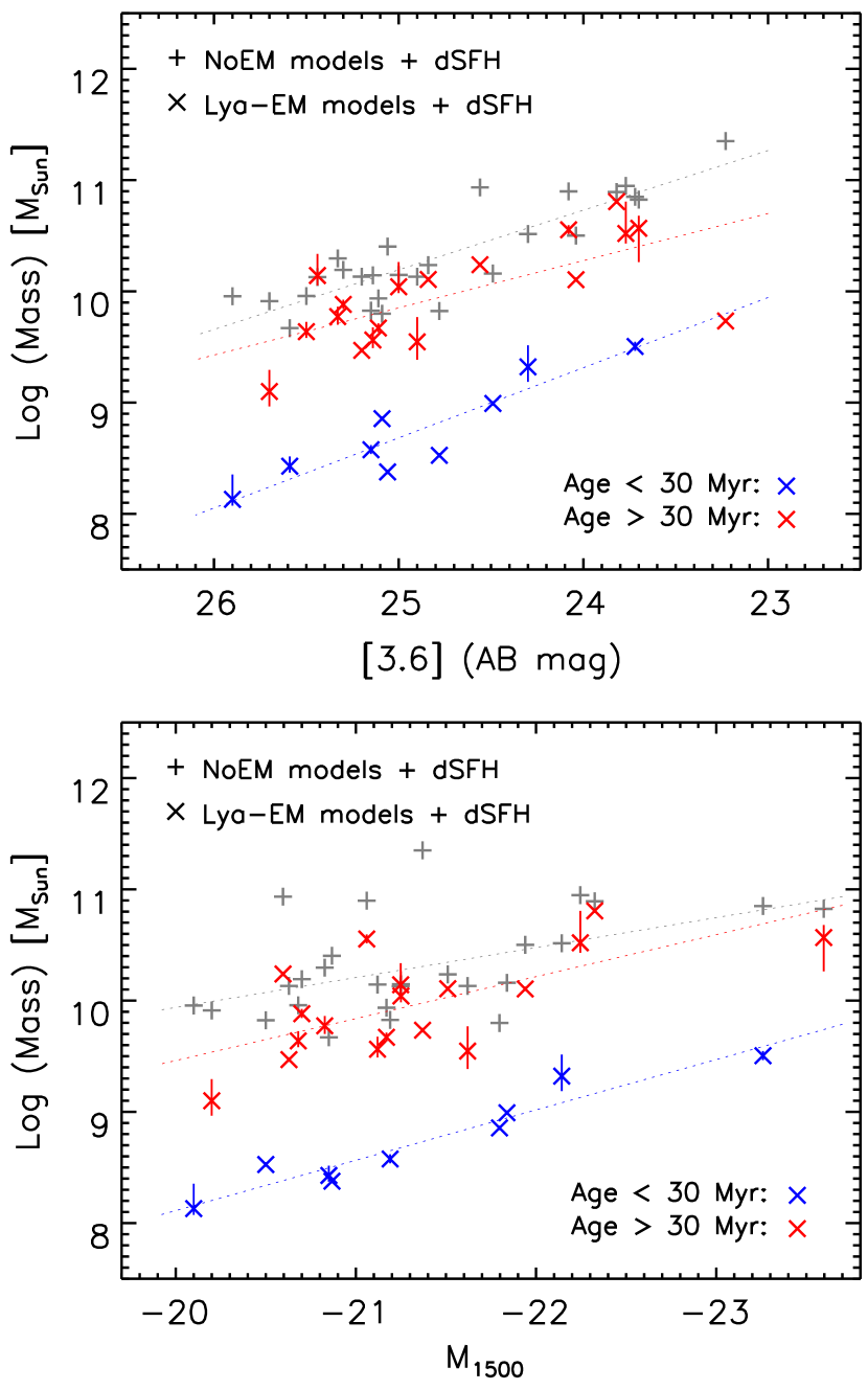
Figure 7.— The same as Figure 6, but for dSFH.

4.2. Age

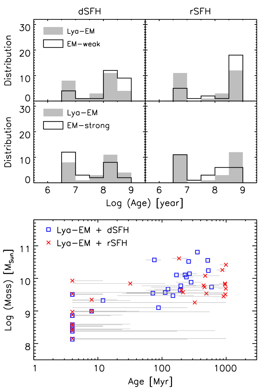
Figure 8.— Ages derived from models with different nebular emission. The filled grey histograms show the age distributions from the Ly$\alpha$-EM models. The black unfilled histograms represent the age distributions from the EM-weak models (top two panels) and the EM-strong models (middle two panels). The distributions of the different models look similar. The bottom panel shows the relation between age and stellar mass derived from the Ly$\alpha$-EM models. The grey horizontal bars indicate the $1\sigma$ uncertainties. Note that we only show the uncertainty in the age direction and choose the best-fit mass; in reality there is a strong degeneracy between the two. For the purpose of clarity, the symbols for the rSFH models have been shifted by 0.02 along the y-axis. Many galaxies are older than 200–300 Myr, with stellar masses close to, or higher than $10^{10}\,M_{\sun}$. Meanwhile, a significant fraction of the galaxies are dominated by extremely young stellar populations with ages of several Myr.

As already mentioned, the age of a stellar population is usually poorly constrained from SED modeling, especially for high-redshift galaxies with only 3–5 photometric data points. During our SED fitting, we allowed the age to vary between 4 and 1000 Myr. Figures 1 and 4 show that the stellar populations derived from the NoEM models are mostly older than 100 Myr. The inclusion of nebular emission largely reduces the derived age, leading to extremely young (a few Myr) stellar populations in some galaxies. Figure 8 compares the ages derived from models with different nebular emission. The filled grey histograms show the age distributions from the Ly$\alpha$-EM models. The black unfilled histograms represent the age distributions from the EM-weak models (top two panels) and the EM-strong models (middle two panels). The distributions of the different models look similar. They all appear to show bimodal distributions. This bimodality could be real, but it could also be caused by selection effects (or sample bias) and modeling limitations. Our galaxies were selected to have strong Ly$\alpha$ emission, which is biased towards younger populations. They were further limited by the IRAC 1 detections, which is biased towards higher stellar masses (older populations) and/or those with strong nebular lines. A full exploration requires a complete, mass-limited sample in this redshift range. The other reason for the bimodality is modeling limitations. The minimum age allowed by our models is 4 Myr, so galaxies younger than 4 Myr would have a measured age of 4 Myr. In addition, these measured ‘young’ ages usually have large uncertainties (typically 20$\sim$30 Myr), as shown in the bottom panel of Figure 8. Therefore, the actual age distribution could be more smooth.

Despite the selection effects and the measurement uncertainties of the ages, we may divide our sample into two subsamples, based on Figures 4 and 8. One consists of old galaxies with ages of several hundred Myr, and the other one includes young galaxies that are mostly only several Myr old. They are referred to as ‘old’ and ‘young’ subsamples in section 4.1. The bottom panel in Figure 8 shows the relation between age and stellar mass derived from the Ly$\alpha$-EM models. It suggests that slightly more than half of the galaxies are a few hundred Myr old. In particular, ages in some galaxies from the rSFH models are older than 300–500 Myr. These galaxies usually have masses close to or higher than $10^{10}\,M_{\sun}$ (up to $10^{11}\,M_{\sun}$). These massive and old galaxies already appear to exist when the universe was only 0.8–1.0 Gyr old.

Meanwhile, Figure 8 also shows the existence of extremely young galaxies in our sample. Both dSFH and rSFH models suggest that some galaxies are only several Myr old. These galaxies are usually less massive, with masses between $10^{8}$ and $3\times 10^{9}\,M_{\sun}$. Pirzkal et al. (2007) found that some LAEs at $4<z<5.7$ in the Hubble Ultra Deep Field are very young (a few Myr old) with masses between $10^{6}$ and $10^{8}\,M_{\sun}$. The young galaxies in our sample are similar to these galaxies in terms of age, but are certainly more massive. This implies that extremely young galaxies at high redshift already have a wide range of stellar masses.

4.3. Dust Extinction

The bottom panels of Figures 1 and 4 display the distributions of dust reddening $E(B-V)$. Unlike age and stellar mass, the $E(B-V)$ values derived from different models, including EM models and NoEM models, are consistent. They clearly suggest that the majority of the galaxies in our sample have little or no dust extinction. This is indeed expected. In Paper I, we reported that our galaxies have steep rest-frame UV slopes on average, with a median value of $\beta\sim-2.3$. Since the UV slope is very sensitive to dust extinction, such steep slopes already indicate little dust extinction. The results are also broadly compatible with recent observations (e.g. Walter et al., 2012; Ouchi et al., 2013; Ota et al., 2014; Willott et al., 2015). Several galaxies in our sample have moderate dust extinction with $E(B-V)>0.1$. These galaxies are relatively massive with masses higher than $10^{9}\,M_{\sun}$.

4.4. Mass-SFR Relation

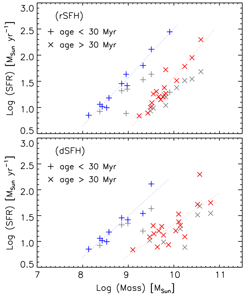
Figure 9.— The stellar mass - SFR relations, derived from the Ly$\alpha$-EM models with rSFH (upper panel) and dSFH (lower panel). The pluses and crosses represent the young and old subsamples, respectively. The grey symbols indicate the SFRs calculated from the UV continuum (without correction for dust extinction) in Paper I. The blue and red symbols indicate the SFRs corrected for dust extinction. The dotted lines are the best linear (in the log space) fits to the data points. The stellar masses are taken from the Ly$\alpha$-EM models with rSFH. The two subsamples show a tight mass-SFR relation, with slopes close to 1. The tight relation is likely caused by the combination of the intrinsic mass-SFR relation, selection effects, and relatively small parameter space that two subsamples occupy.

In low-redshift star-forming galaxies, there is a correlation between stellar mass and SFR, in which SFR is higher in more massive galaxies (e.g. Daddi et al., 2007; Elbaz et al., 2007; Noeske et al., 2007). This relation is referred to as the ‘main sequence’ of star-forming galaxies. It evolves with redshift so that the normalization of the relation at higher redshift is higher (at least for the redshift range $z\leq 2-3$). The mass-SFR relation usually applies to massive galaxies with $M_{\ast}\geq 10^{9}$ $M_{\sun}$, corresponding to the old subsample in Figures 6 and 8. In addition, starburst galaxies such as ULIRGs and SMGs may reside well above the relation.

Figure 9 shows the mass-SFR relations for our galaxies, derived from the Ly$\alpha$-EM models with rSFH (upper panel) and dSFH (lower panel). The pluses and crosses represent the young and old subsamples, respectively. The grey symbols indicate the SFRs calculated from the UV continuum (without correction for dust extinction) in Paper I. We correct for dust extinction using the $E(B-V)$ values in Table 3 based on the Calzetti (2000) law. The results are shown as blue and red symbols. The correction is large only for the most massive galaxies in each subsample, which show moderate dust extinction as seen in section 4.3. The two subsamples both show a tight mass-SFR relation. In the upper panel for rSFH, the linear Pearson correlation coefficients for the old and young subsamples are 0.95 and 0.99, respectively. The coefficients in the lower panel for dSFH are 0.77 and 0.95. The slopes are close to 1, consistent with the results from simulations (e.g. Finlator et al., 2011). It also agrees with the slopes found in lower-redshift galaxies (e.g. Guo et al., 2013; Sparre et al., 2015). The slope of $\sim 1$ indicates that the specific SFRs (sSFRs) are similar within either subsample. However, the average sSFR of the young subsample is much higher than that of the old subsample, so that the two subsamples are well separated in the mass-SFR diagram. This is because the two subsamples cover the similar range of SFRs, but the old subsample is ten times more massive on average.

The correlation in either subsample is tight, due to the combination of a few reasons, including the intrinsic mass-SFR relation, the selection effects, and the relatively small parameter space that either subsample occupies. In particular, the correlation for the ‘young’ subsample is very tight, mainly because of their extremely young ages. The GALEV model outputs start from 4 Myr in steps of 4 Myr. The ages measured in the ‘young’ subsample are mostly 4 Myr and 8 Myr, and thus these ‘young’ galaxies have not evolved considerably.

Figure 10 shows the sSFR as a function of redshift, taken from Madau & Dickinson (2014) (and references therein). It illustrates the efficiency of stellar mass growth in galaxies across cosmic time. The sSFR increases rapidly from the local Universe to $z\sim 2$, and then flattens (or slightly climbs) towards higher redshifts. We focus on the high-redshift range. The $z\geq 4$ data points in the figure were from two LBG samples of Stark et al. (2013) and González et al. (2014). Our results are displayed as a blue circle (young subsample) and a red circle (old subsample). The horizontal error bars indicate the redshift range, and the vertical error bars indicate the $2\sigma$ range of the object number distribution (i.e., inclusion of 95% of the objects). The average sSFR of the old subsample agrees well with the two previous studies Stark et al. (2013) and González et al. (2014). Note that in these studies nebular emission lines were also incorporated during their SED modeling. In addition, the mass-SFR relation of the old subsample is well consistent with the simulation of Finlator et al. (2011). All these suggest that the galaxies in our old subsample are ‘normal’ star-forming galaxies at $z\geq 6$. The sSFRs of the old subsample are roughly consistent with (or marginally higher than) those at $z\sim 2$, suggesting that the efficiency of stellar mass growth did not change much in the most time of the first 3 Gyr.

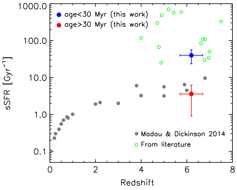
Figure 10.— The sSFR as a function of redshift. The grey circles represent the data points taken from Madau & Dickinson (2014) (and references therein). The open green circles represent some of high-sSFR galaxies at $z>4$ taken from the literature (Pirzkal et al., 2007; Bowler et al., 2012; Finkelstein et al., 2013; Huang et al., 2015). Our results of the median sSFRs are displayed as a blue circle (young subsample) and a red point (old subsample). The horizontal error bars indicate the redshift range, and the vertical error bars indicate the $2\sigma$ range of the object number distribution (i.e., inclusion of 95% of the objects). The sSFR of the old subsample is consistent with previous studies compiled by Madau & Dickinson (2014), following the main sequence of star-forming galaxies. The sSFR of the young subsample is well above the main sequence, presumably due to starburst activity in these galaxies. Such galaxies are not rare at high redshift, as seen from the open circles.

The average sSFR of the young subsample is about ten times higher than the relation defined by previous studies. It has been clear that galaxies with strong starburst activity at $z\leq 2$ are well above ($\geq 10$ times) the main sequence of star-forming galaxies (e.g. Rodighiero et al., 2011; Sargent et al., 2012). So the young subsample seems to be the high-redshift counterparts of $z\leq 2$ starbursts. The fraction of such starbursts at $z\leq 2$ is very low, while in our sample this fraction is much higher, partly due to selection effects. On the other hand, galaxies with very high sSFRs at high redshift are not rare. Section 5.3 provides more discussion on this topic.

The bimodal distribution of ages and sSFRs seen in Figures 8 and 9 were largely explained by selection effects and modeling limitations in the above sections, though we cannot rule out the possibility of an intrinsic bimodality. Such bimodality has been reported for galaxies at $2.5<z<3.5$ by Kajisawa et al. (2010), who found that the sSFRs in their low-sSFR and high-sSFR galaxies are 0.5–1.0 Gyr^-1 and $\sim$10 Gyr^-1, respectively. This suggests that the bimodality seen in our sample may partially reflect a real bimodal distribution of sSFRs.

5. DISCUSSION

5.1. Testing Ly$\alpha$-EM Models

It is clear that SED modeling of high-redshift galaxies can be largely affected by the presence of strong nebular emission. For galaxies at $6\leq z<7$, the existence of strong lines is often evidenced by their IRAC 1 flux excess (compared to the IRAC 2 flux). This is because in this redshift range, the IRAC 1 band covers some of the strongest lines such as [O iii], H$\alpha$, and H$\beta$. A significant fraction of galaxies at $z\geq 6$, including photometrically selected and spectroscopically confirmed galaxies, show a strong IRAC 1 flux excess (e.g. González et al., 2010; McLure et al., 2011; Curtis-Lake et al., 2013). In fact, many galaxies in our sample also show such an excess. At $z>7$, galaxies with strong nebular lines start to show red IRAC [3.6]–[4.5] colors (e.g. Roberts-Borsani et al., 2015; Zitrin et al., 2015).

The contribution of nebular emission to the IRAC 1 and 2 bands can be large or dominant. Stark et al. (2013) showed that the mean rest-frame EW of H$\alpha$ at high redshift is a few hundred Å. Smit et al. (2015) showed some extreme cases of strong emission lines by searching for $z=6.6-6.9$ galaxies with very blue IRAC [3.6]–[4.5] colors. Over a small redshift range $z=6.6-6.9$, the IRAC 1 band covers [O iii] and H$\beta$, but the IRAC 2 band does not cover any strong emission lines. The galaxies that they found have very large rest-frame EW of [O iii]+H$\beta$ in the range of 900 to $>2000$ Å, with a median value of $\sim 1400$ Å. In these galaxies line emission dominates the IRAC 1 photometry. Therefore, it is expected that the galaxies in our sample have strong nebular lines.

Our analysis was mostly based on the Ly$\alpha$-EM models. When we computed the Ly$\alpha$-EM models from the GALEV-EM models in section 3, we scaled nebular emission lines using the observed Ly$\alpha$ flux. Figure 11 shows the distribution of the derived scaling factors. They cover a range from 0.6 to 3.5, with a median value 1.6. It is expected that line emission derived from the Ly$\alpha$-EM models is stronger than that from the GALEV-EM models, because our galaxies were selected to have strong line emission. The scaling factors span a relatively small range (within a factor of $\sim$2 around the median value 1.6), suggesting that the dynamic range of the EM-strong and EM-weak models is large enough to sample the majority of high-redshift galaxies.

Figure 11.— Distribution of the scaling factors of nebular line strength derived for the Ly$\alpha$-EM models. The Ly$\alpha$-EM models were computed from the GALEV-EM models by scaling nebular emission lines to match the observed Ly$\alpha$ flux (section 3). The derived scaling factors cover a range from 0.6 to 3.5, with a median value 1.6.

We may test our Ly$\alpha$-EM models using a few ‘special’ galaxies (Figure 12) not in our sample. These galaxies are spectroscopically confirmed with measured Ly$\alpha$ line flux, so that we can estimate nebular emission from their Ly$\alpha$ emission based on the Ly$\alpha$-EM models. In addition, they are at certain redshift ranges so that one of the two IRAC bands covers strong nebular emission, but the other one does not. In this case, the difference of the photometry between the two bands roughly reflects the strength of nebular lines. The first two galaxies (a and b in Figure 12) are at $z=6.74$ and $z=6.76$ found by Clément et al. (in preparation) and by Huang et al. (2015), respectively. In these two galaxies, the IRAC 1 band covers H$\beta$ and [O iii], while the IRAC 2 band does not cover any strong lines. The other two galaxies in Figure 12 are the one at $z=7.51$ from Finkelstein et al. (2013) and the one at $z=7.73$ from Oesch et al. (2015). For these two galaxies, the IRAC 2 band covers H$\beta$ and [O iii], and the IRAC 1 band does not cover strong lines.

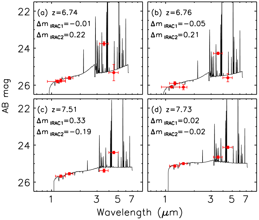
Figure 12.— SED modeling of four galaxies taken from the literature to test our Ly$\alpha$-EM models. These galaxies are spectroscopically confirmed with measured Ly$\alpha$ line flux. They are at certain redshift ranges so that one of the two IRAC bands covers strong nebular emission, but the other one does not. We also show the difference between the observed and model photometry in the IRAC bands ($\Delta m_{\rm IRAC1}$ and $\Delta m_{\rm IRAC2}$). The fitting results for all the galaxies except (c) are good, and their magnitude difference values are smaller than the corresponding photometric uncertainties ($1\sigma$) in the IRAC 1 and IRAC 2 bands. The best fit to galaxy (c) is not acceptable ($\chi_{r}^{2}\gg 1$), due to the reason that the nebular lines (scaled from Ly$\alpha$) in the model spectra are not strong enough to account for the large difference between the IRAC 1 and IRAC 2 photometry. This is because its Ly$\alpha$ emission has been largely attenuated by the highly neutral IGM at very high redshift.

We perform SED modeling for the four galaxies based on the Ly$\alpha$-EM models with rSFH. The fitting results for galaxies (a) and (d) are very good ($\chi_{r}^{2}\leq 1$). We are not able to obtain acceptable results for galaxies (b) and (c), due to the reason that the nebular lines (scaled from Ly$\alpha$) in the model spectra are not strong enough to account for the large difference between the IRAC 1 and IRAC 2 photometry. We note that the Ly$\alpha$ emission line in galaxy (b) is located on one of strong sky OH lines, and its flux measurement could be significantly affected, as pointed out by the discovery paper (Huang et al., 2015). Nevertheless, we re-model the SEDs for galaxies (b) and (c) using the EM-strong models, and obtain a reasonable fit for galaxy (b). For galaxy (c), however, we fail to achieve an acceptable fit ($\chi_{r}^{2}\gg 1$). The best fitting results for the four galaxies are plotted in Figure 12, in which we also show the difference between the observed and model photometry in the IRAC bands ($\Delta m_{\rm IRAC1}$ and $\Delta m_{\rm IRAC2}$). For all the galaxies except (c), these magnitude difference values are smaller than the corresponding photometric uncertainties ($1\sigma$) in the IRAC 1 and IRAC 2 bands.

Galaxy (c) has very weak Ly$\alpha$ emission (compared to its other nebular lines), as already noted by Finkelstein et al. (2013). At $z=7.51$, the IGM is much more neutral than that at $z\sim 6$, so Ly$\alpha$ emission can be largely attenuated by the neutral IGM or eaten by Ly$\alpha$ damping wings (e.g. Miralda-Escudé, 1998). In other words, the ratio of intrinsic to observed Ly$\alpha$ flux is a function of redshift, as we mentioned in the previous section. So our assumption about this ratio is no longer valid. Recent simulations suggest that the Ly$\alpha$ damping wing owing to patchy reionization should be fairly uniform at a given redshift (Mesinger et al., 2015). In this case, our ability to fit galaxy (d) but not (c) is not likely to reflect incomplete reionization. Instead, it may indicate scatter in the level of attenuation of self-shielded systems or in the intrinsic properties of the galaxies’ interstellar media.

In summary, three out of the four galaxies can be well fit with our Ly$\alpha$-EM or EM-strong models. We were not able to obtain a reasonable fit for the galaxy at $z=7.51$, due to the limitation (redshift coverage) of our models. The tests above show that our models can provide reasonable SED modeling for high-redshift galaxies with nebular emission taken into account.

5.2. ‘Young’ and ‘Old’ Populations

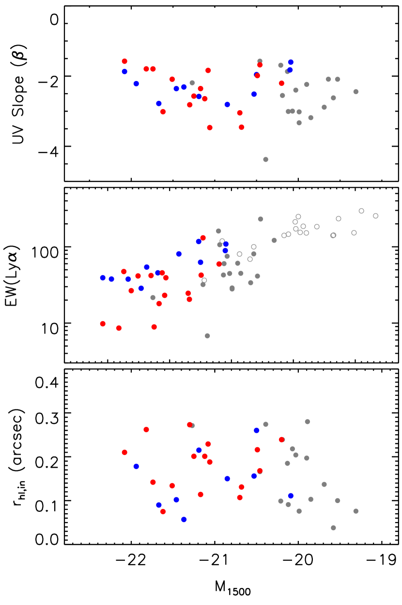
Figure 13.— Physical properties of the ‘young’ and ‘old’ subsamples as a function of rest-frame UV luminosity $M_{1500}$. The blue and red circles represent the ‘young’ and ‘old’ galaxies, respectively. The grey circles (including filled and open circles) represent the galaxies that are not included for analysis in this paper. The top panel shows the rest-frame UV slope $\beta$ derived in Paper I. The two subsamples have similar mean slopes. The middle panel shows the rest-frame Ly$\alpha$ EW derived in Paper I. The ‘young’ galaxies have relatively higher Ly$\alpha$ EWs than the ‘old’ ones. The bottom panel shows the half-light radii $r_{hl,in}$ estimated in Paper II. The average radii of the two subsamples are roughly consistent.

In section 4 we identified two subsamples in our galaxies, one ‘old’ subsample with ages of several hundred Myr and one ‘young’ subsample with ages of several Myr. Either subsample follows a tight stellar mass-SFR relation. The mean sSFR of the ‘old’ subsample is consistent with those in many high-redshift galaxies reported in the literature, while the mean sSFR of the ‘young’ subsample is an order of magnitude higher. In Figure 13 we compare the two subsamples in the context of physical properties as a function of rest-frame UV luminosity $M_{1500}$. These physical quantities (including rest-frame UV slopes, Ly$\alpha$ EWs, and half-light radii) were measured in Papers I and II. Their measurements are usually associated with considerable uncertainties (see Papers I and II), which are not plotted in the figure for the purpose of simplicity. The blue and red circles represent the ‘young’ and ‘old’ galaxies, respectively. The grey circles (including filled and open circles) represent the galaxies that are not included for analysis in this paper.

The top panel of Figure 13 shows the rest-frame UV slope $\beta$ as a function of $M_{1500}$. The median and standard deviation values of the slopes for the young and old subsamples are $-2.31\pm 0.40$ and $-2.20\pm 0.62$, respectively. They are consistent. UV slopes are most sensitive to dust extinction. As we have seen in section 4.3, there is little dust extinction in these galaxies except for several of the most massive galaxies. So the ‘young’ galaxies do not show bluer slopes than the ‘old’ galaxies.

The middle panel of Figure 13 shows the rest-frame Ly$\alpha$ EW as a function of $M_{1500}$. The median and standard deviation values of the EWs for the two subsamples are $54.2\pm 30.7$ and $39.3\pm 29.5$, respectively. The ‘young’ galaxies have relatively higher Ly$\alpha$ EWs than the ‘old’ ones. A Ly$\alpha$ EW is the ratio of the Ly$\alpha$ line flux to the continuum flux. The Ly$\alpha$ line strength measures the strength of nebular lines, especially in our Ly$\alpha$-EM models. We expect to see stronger nebular lines in younger systems. So this panel reflects that a galaxy with stronger Ly$\alpha$ line emission tend to be younger.

The bottom panel shows the half-light radii $r_{hl,in}$ (at rest-frame $\sim$1800 Å) as a function of $M_{1500}$. The radii have been corrected for PSF broadening with simulations. The median and standard deviation values of the radii for the two subsamples are $0.15\pm 0.06$ and $0.20\pm 0.06$, respectively. The old galaxies are marginally larger on average. However, it is not straightforward to compare the sizes of the two subsamples. At lower redshift, there is a mass-size relation, in which more massive galaxies (the ‘old’ subsample in our case) tend to be larger. On the other hand, the galaxies in our ‘young’ subsample may have strong starburst activity as indicated by their high sSFRs. A significant fraction of low-redshift starbursts are mergers, which tend to have large sizes.

5.3. Comparison with Previous Studies

There are a number of studies on the stellar populations of $z\geq 6$ galaxies in the literature. The majority of these galaxies are photometrically selected LBGs. There was little study for $z\geq 6$ LAEs. As we explained in Introduction, almost all the known LAEs were discovered by ground-based telescopes, and did not have deep infrared observations. Our program provides the largest sample so far for studying stellar populations in spectroscopically confirmed LAEs at $z\geq 6$.

Direct comparison with previous studies is very difficult if not impossible, because different studies use different galaxy samples (selected from different datasets with different selection criteria) and SED modeling methods. We mainly focus on two questions: whether extremely young populations have been reported, and whether previously reported sSFRs cover a wide range that agrees with our ‘young’ and ‘old’ subsamples. As we emphasized earlier, age is poorly constrained from SED modeling, so here we broadly define ‘extremely young galaxies’ as those with the best-fitting ages younger than $\sim 30$ Myr, like the galaxies in our ‘young’ subsample.

In the previous studies of photometrically-selected LBGs, extremely young galaxies have been rarely reported. The majority of these LBGs tend to have relatively old and mature populations with ages of a few hundred or several tens Myr, from SED fitting without nebular emission taken into account. When nebular emission were considered (especially in models with smoothly-varying SFHs), however, extremely young populations were required to explain the SEDs of some LBGs (Schaerer & de Barros, 2010; McLure et al., 2011; Curtis-Lake et al., 2012; Huang et al., 2015). For example, McLure et al. (2011) selected a sample of $z>6$ LBGs from $HST$ deep fields, and found that these galaxies were mostly a few hundred Myr old if nebular emission was not included in their SED modeling. When nebular emission was added, about 25% of their LBGs with IRAC 1 detections were found to be extremely young, with a median age of 9 Myr.

In the previous studies of high-redshift LAEs, extremely young galaxies were found to be common. For example, Ono et al. (2010) stacked a large number of photometrically-selected LAEs at $z\sim 5.7$ and 6.5, and performed SED modeling on the stacked LAEs. Despite that the measurements from stacked data could be unreliable (e.g. Vargas et al., 2014), they found that these LAEs have ages of only 1-3 Myr, little dust extinction, and strong nebular emission. In the sample of Pirzkal et al. (2007), there are nine spectroscopically confirmed LAEs at $z\sim 5$. Most of them were found to be younger than 10 Myr. These results are quite consistent with ours.

The sSFRs in our galaxies span a quite large range. Their values are about 3–4 Gyr^-1 in the ‘old’ subsample, which is consistent with previous studies such as Curtis-Lake et al. (2012), Stark et al. (2013), and González et al. (2014). The sSFRs in our ‘young’ subsample are about an order of magnitude higher, likely due to starburst activity in these galaxies. Such high sSFRs are indeed also common in previous studies. For example, in a sample of seven secure high-redshift LBGs by Bowler et al. (2012), three of them were found to have sSFRs around 4–5 Gyr^-1, and another three have sSFRs close to or higher than 30 Gyr^-1. These numbers roughly agree with those found in our ‘old’ and ‘young’ subsamples. Some studies have reported even stronger starbursts in $z>6$ galaxies, with sSFRs between one hundred and several hundred Gyr^-1 (e.g. Ono et al., 2010; Finkelstein et al., 2013; Huang et al., 2015). In Figure 10, the green circles represent some of high-sSFR galaxies from Pirzkal et al. (2007), Bowler et al. (2012), Finkelstein et al. (2013), and Huang et al. (2015). Galaxies ($4<z<6$) from Pirzkal et al. (2007) all have very high sSFRs, and are included in Figure 10. All these above suggest that strong starburst activity is common in very high-redshift galaxies.

5.4. LAEs and LBGs

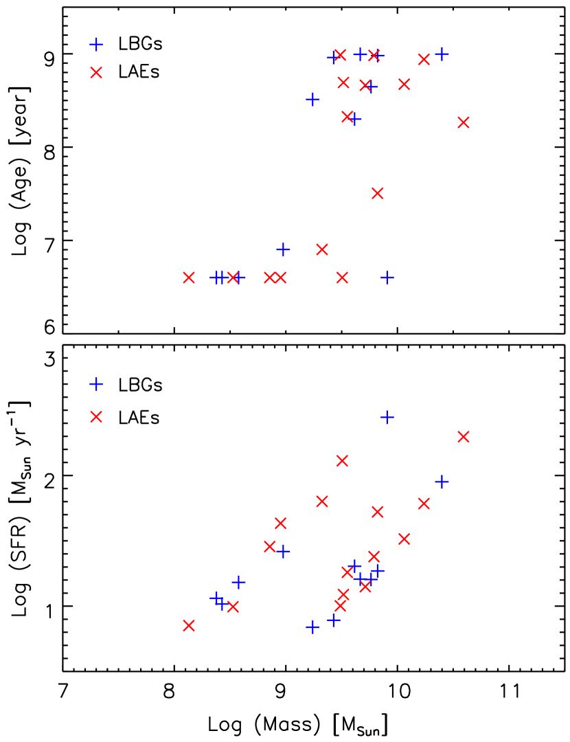
Figure 14.— The measured ages and SFRs as a function of stellar mass for the LAEs and LBGs in our sample. The minimum age allowed in our models is 4 Myr, and some ages in the upper panel are at this limit. The distributions of the LBGs and LAEs in the age-mass and SFR-mass diagrams are indistinguishable. The number ratios of the LAEs to LBGs agree with each other in the ‘young’ and ‘old’ subsamples.

In this series of papers (including this paper and Papers I and II), LAEs are defined as galaxies found by the narrow-band (or Ly$\alpha$) technique, and LBGs are defined as galaxies found by the dropout technique. As we already pointed out in Papers I and II, this widely-used classification only reflects the methodology that we apply to select galaxies. It does not mean that the two types of galaxies are intrinsically different. Another definition of LAEs is based on the Ly$\alpha$ EW, e.g., a galaxy is a LAE if its Ly$\alpha$ EW is greater than 20 Å. This definition is physically more meaningful, but observationally difficult, because one can easily obtain a flux-limited sample, not a EW-limited sample. In addition, it is meaningless for broad-band selected galaxies. So we use the former definition.

It is not entirely clear whether high-redshift LAEs and LBGs represent physically different populations. Direct comparison between LAEs and LBGs is difficult because of the very different target selection procedures. As we already explained in Papers I and II, the LAEs in our original sample of 67 galaxies are composed of a well-defined sample in terms of Ly$\alpha$ flux. On the other hand, the LBGs in the sample only represent the LBGs with strong Ly$\alpha$ emission since they are spectroscopically confirmed. In Papers I and II, we compared the LAEs and LBGs in our sample in great details, and found that the two populations are indistinguishable in all aspects of physical properties that we considered, including the Ly$\alpha$ emission strength, UV continuum properties, sizes, and morphology, etc.

Figure 14 shows the distributions of the measured stellar masses, ages, and SFRs for the LAEs and LBGs in our sample of 27 galaxies used in this paper. The blue pluses and the red crosses represent the LBGs and LAEs, respectively. The distributions of the LBGs and LAEs in the age-mass and SFR-mass diagrams are indistinguishable. In particular, there are 6 LAEs and 5 LBGs in the ‘young’ subsample, and there are 9 LAEs and 7 LBGs in the ‘old’ subsample. The number ratios of the LAEs to LBGs nicely agree with each other in the two subsamples. All these are consistent with our previous conclusion that the LAEs and LBGs in our sample have common properties, suggesting that LAEs are a subset of LBGs with strong Ly$\alpha$ emission lines. The conclusion is also consistent with recent simulations (e.g. Dayal & Ferrara, 2012; Garel et al., 2015).

5.5. Prospect for Spectroscopic Follow-up with JWST

Currently there are two ways to assess the strength of rest-frame optical nebular emission lines and use that information to derive the physical properties of underlying stellar population in $z>6$ galaxies: (1) to observe galaxies in specific redshift ranges where one of the IRAC band is line-free (e.g., $6.6<z<6.9$ galaxies as studied by Smit et al. (2014)), and (2) to model emission-line strengths based on the measured Ly$\alpha$ lines (this work). The first method is more direct and accurate, but because of the stringent constraints on redshift, the number of galaxies that can be studied is rather small. The second method suffers from relatively large uncertainties, but can be applied to a much larger sample of $z>6$ galaxies as we have shown in this paper.

Although the above is the best we can do at the moment, we note that we are actually on the verge of a breakthrough as the JWST becomes available and changes the emphasis from photometry to spectroscopy. Figure 15 shows the flux distributions of the [O III] 5007 Å and H$\alpha$ lines predicted by the modeling described in this paper. The figure shows that we should be able to detect almost all these lines with a line-flux sensitivity of $\sim 10^{-17}$ ergs cm^-2 s^-1. Based on the JWST Prototype Exposure Time Calculator (ETC), such a sensitivity will be easily reachable with NIRSpec. For example, to achieve a 5$\sigma$ detection (per resolution element) of an [O III] 5007Å line at $z=6.5$ with a line flux of $10^{-17}$ ergs cm^-2 s^-1, the required integration time will be only $\sim 500$ seconds. The corresponding integration time for H$\alpha$ (i.e., at $z=6.5$ and with a line flux of $10^{-17}$ ergs cm^-2 s^-1) will be $\sim 800$ seconds. These numbers clearly indicate that with JWST/NIRSpec, it will be easy to detect [O III] and H$\alpha$ lines with the brightest $z>6$ galaxies like those we have studied here. In fact, NIRSpec has the sensitivity to detect much fainter lines, making these bright $z>6$ SDF galaxies ideal targets for a detailed NIRSpec spectroscopic study. In several years, such a study will be able to test the validity of the results presented here, and will undoubtedly make many more interesting discoveries.

Figure 15.— Flux distributions of the [O III] 5007 Å and H$\alpha$ lines predicted by the modeling described in this paper. The flux was calculated based on the JWST prototype ETC (version P1.6), available at http://jwstetc.stsci.edu. The following parameters were used with the NIRSpec ETC: Filter/Grating $=$ G395H/F290LP; $R=2700$; MSA shutter $=$ 0$\farcs$2 $\times$ 0$\farcs$45; Flat continuum in F$\nu$; FWHM = 40 Å $\sim$ 300 km s^-1 at 3.755 $\mu$m for [O III], or FWHM = 50 Å $\sim$ 300 km s^-1 at 4.922 $\mu$m for H$\alpha$. The continuum normalization was set to be 30 AB mag at 3.6 $\mu$m, so that the S/N calculation is essentially driven by the line flux. With JWST/NIRSpec, it will be easy to detect [O III] and H$\alpha$ lines in bright $z>6$ galaxies.

6. SUMMARY

This paper is the third in a series presenting the physical properties of a large sample of 67 spectroscopically confirmed galaxies at $z\geq 6$. The sample consists of 51 LAEs at $z\simeq 5.7$, 6.5, and 7.0, and 16 LBGs at $5.9\leq z\leq 6.5$. They have deep optical imaging data from Subaru, near-IR data from $HST$, and mid-IR data from $Spitzer$. In this paper, we have reported a detailed study of stellar populations in these galaxies. We have focused on a subsample of 27 galaxies with $Spitzer$ IRAC 1 detections at 3.6 $\mu$m. This subsample represents luminous and massive galaxies with strong Ly$\alpha$ emission at $z\geq 6$. We used the wealth of the multi-band data and the secure Ly$\alpha$ redshifts and flux to model the SEDs of the 27 galaxies and characterize their stellar populations.

We used the GALEV evolutionary synthesis models with nebular continuum and line emission to mainly constrain three physical parameters: age, stellar mass, and dust extinction. We adopted two representative SFHs, an exponentially declining SFH (dSFH) and a smoothly rising SFH (rSFH). We mostly used the latter two SFHs in our analysis. In order to incorporate nebular emission, we scaled the nebular emission from the GALEV models to match the observed Ly$\alpha$ flux (the Ly$\alpha$-EM models) under two simple assumptions. With the Ly$\alpha$-EM models, we were able to nicely break the strong degeneracy of model spectra between young galaxies with prominent nebular emission and mature galaxies with strong Balmer breaks.

Our best-fitting results show that the galaxies in our sample has a wide range of SED ages from several Myr to a few hundred Myr. They also have a wide range of stellar masses from $\sim 10^{8}$ to $\sim 10^{11}\,M_{\sun}$. Interestingly, the distribution of the measured ages (despite the large uncertainties) appear to be bimodal, likely due to selection effects and modeling limitations (though we cannot rule out the possibility of an intrinsic bimodality). Based on this bimodality, we divided the galaxies into two subsamples: an ‘old’ subsample and a ‘young’ subsample. The ‘old’ subsample mainly consists of galaxies older than 100 Myr, with stellar masses higher than $10^{9}\,M_{\sun}$. Many galaxies are older than 300–500 Myr. The ‘young’ subsample consists of galaxies younger than 30 Myr (usually several Myr old). These galaxies are less massive, with masses ranging between $\sim 10^{8}$ and $\sim 3\times 10^{9}\,M_{\sun}$. The majority of the galaxies both subsamples show little or no dust extinction, as already hinted by their steep rest-frame UV slopes.

Both subsamples show a correlation between stellar mass and SFR, but with very different normalizations. The mean sSFR of the ‘old’ subsample is about 3–4 Gyr^-1, consistent with the mass-SFR relation defined by previous studies. The mean sSFR of the ‘young’ subsample is an order of magnitude higher. Such higher sSFRs have also been frequently reported in previous studies. They are likely due to starburst activity in these galaxies. Finally, the LAEs and LBGs in our sample are indistinguishable in all physical properties that we have considered, suggesting that LAEs are a subset of LBGs with strong Ly$\alpha$ emission lines.

References

- Ashby et al. (2013) Ashby, M. L. N., Willner, S. P., Fazio, G. G., et al. 2013, ApJ, 769, 80
- Bouwens et al. (2014) Bouwens, R. J., Illingworth, G. D., Oesch, P. A., et al. 2014, ApJ, 793, 115
- Bouwens et al. (2015) Bouwens, R. J., Illingworth, G. D., Oesch, P. A., et al. 2015, ApJ, in press
- Bowler et al. (2012) Bowler, R. A. A., Dunlop, J. S., McLure, R. J., et al. 2012, MNRAS, 426, 2772
- Bruzual & Charlot (2003) Bruzual, G., & Charlot, S. 2003, MNRAS, 344, 1000
- Cai et al. (2014) Cai, Z.-Y., Lapi, A., Bressan, A., et al. 2014, ApJ, 785, 65
- Calzetti et al. (2000) Calzetti, D., Armus, L., Bohlin, R. C., et al. 2000, ApJ, 533, 682
- Conroy (2013) Conroy, C. 2013, ARA&A, 51, 393
- Curtis-Lake et al. (2012) Curtis-Lake, E., McLure, R. J., Pearce, H. J., et al. 2012, MNRAS, 422, 1425
- Curtis-Lake et al. (2013) Curtis-Lake, E., McLure, R. J., Dunlop, J. S., et al. 2013, MNRAS, 429, 302
- Curtis-Lake et al. (2015) Curtis-Lake, E., McLure, R. J., Dunlop, J. S., et al. 2015, MNRAS, submitted
- Daddi et al. (2007) Daddi, E., Dickinson, M., Morrison, G., et al. 2007, ApJ, 670, 156
- Dayal & Ferrara (2012) Dayal, P., & Ferrara, A. 2012, MNRAS, 421, 2568
- Dijkstra (2014) Dijkstra, M. 2014, PASP, 31, 40
- de Barros et al. (2014) de Barros, S., Schaerer, D., & Stark, D. P. 2014, A&A, 563, AA81
- Dunlop et al. (2013) Dunlop, J. S., Rogers, A. B., McLure, R. J., et al. 2013, MNRAS, 432, 3520
- Egami et al. (2005) Egami, E., Kneib, J.-P., Rieke, G. H., et al. 2005, ApJ, 618, L5
- Elbaz et al. (2007) Elbaz, D., Daddi, E., Le Borgne, D., et al. 2007, A&A, 468, 33
- Ellis et al. (2013) Ellis, R. S., McLure, R. J., Dunlop, J. S., et al. 2013, ApJ, 763, LL7
- Eyles et al. (2005) Eyles, L. P., Bunker, A. J., Stanway, E. R., et al. 2005, MNRAS, 364, 443
- Eyles et al. (2007) Eyles, L. P., Bunker, A. J., Ellis, R. S., et al. 2007, MNRAS, 374, 910
- Fan et al. (2001) Fan, X., Narayanan, V. K., Lupton, R. H., et al. 2001, AJ, 122, 2833
- Finkelstein et al. (2013) Finkelstein, S. L., Papovich, C., Dickinson, M., et al. 2013, Nature, 502, 524
- Finlator et al. (2007) Finlator, K., Davé, R., & Oppenheimer, B. D. 2007, MNRAS, 376, 1861
- Finlator et al. (2011) Finlator, K., Oppenheimer, B. D., & Davé, R. 2011, MNRAS, 410, 1703
- Furusawa et al. (2008) Furusawa, H., Kosugi, G., Akiyama, M., et al. 2008, ApJS, 176, 1
- Garel et al. (2015) Garel, T., Blaizot, J., Guiderdoni, B., et al. 2015, MNRAS, 450, 1279
- González et al. (2010) González, V., Labbé, I., Bouwens, R. J., et al. 2010, ApJ, 713, 115
- González et al. (2011) González, V., Labbé, I., Bouwens, R. J., et al. 2011, ApJ, 735, LL34
- González et al. (2014) González, V., Bouwens, R., Illingworth, G., et al. 2014, ApJ, 781, 34
- Grogin et al. (2011) Grogin, N. A., Kocevski, D. D., Faber, S. M., et al. 2011, ApJS, 197, 35
- Guo et al. (2013) Guo, K., Zheng, X. Z., & Fu, H. 2013, ApJ, 778, 23
- Henry et al. (2012) Henry, A. L., Martin, C. L., Dressler, A., Sawicki, M., & McCarthy, P. 2012, ApJ, 744, 149
- Hu et al. (2010) Hu, E. M., Cowie, L. L., Barger, A. J., et al. 2010, ApJ, 725, 394
- Huang et al. (2015) Huang, K.-H., Bradač, M., Lemaux, B. C., et al. 2015, arXiv:1504.02099
- Iye et al. (2006) Iye, M., Ota, K., Kashikawa, N., et al. 2006, Nature, 443, 186
- Jensen et al. (2014) Jensen, H., Hayes, M., Iliev, I. T., et al. 2014, MNRAS, 444, 2114
- Jiang et al. (2008) Jiang, L., Fan, X., Annis, J., et al. 2008, AJ, 135, 1057
- Jiang et al. (2011) Jiang, L., Egami, E., Kashikawa, N., et al. 2011, ApJ, 743, 65
- Jiang et al. (2013a) Jiang, L., Egami, E., Mechtley, M., et al. 2013a, ApJ, 772, 99
- Jiang et al. (2013b) Jiang, L., Egami, E., Fan, X., et al. 2013b, ApJ, 773, 153
- Labbé et al. (2013) Labbé, I., Oesch, P. A., Bouwens, R. J., et al. 2013, ApJ, 777, L19
- Laporte et al. (2015) Laporte, N., Streblyanska, A., Kim, S., et al. 2015, A&A, 575, AA92
- Kajisawa et al. (2010) Kajisawa, M., Ichikawa, T., Yamada, T., et al. 2010, ApJ, 723, 129
- Kashikawa et al. (2004) Kashikawa, N., Shimasaku, K., Yasuda, N., et al. 2004, PASJ, 56, 1011
- Kashikawa et al. (2011) Kashikawa, N., Shimasaku, K., Matsuda, Y., et al. 2011, ApJ, 734, 119
- Kawamata et al. (2015) Kawamata, R., Ishigaki, M., Shimasaku, K., Oguri, M., & Ouchi, M. 2015, ApJ, in press
- Koekemoer et al. (2011) Koekemoer, A. M., Faber, S. M., Ferguson, H. C., et al. 2011, ApJS, 197, 36
- Konno et al. (2014) Konno, A., Ouchi, M., Ono, Y., et al. 2014, ApJ, 797, 16
- Kotulla et al. (2009) Kotulla, R., Fritze, U., Weilbacher, P., & Anders, P. 2009, MNRAS, 396, 462
- Leitherer et al. (1999) Leitherer, C., Schaerer, D., Goldader, J. D., et al. 1999, ApJS, 123, 3
- Madau & Dickinson (2014) Madau, P., & Dickinson, M. 2014, ARA&A, 52, 415
- Malhotra & Rhoads (2002) Malhotra, S., & Rhoads, J. E. 2002, ApJ, 565, L71
- McLure et al. (2011) McLure, R. J., Dunlop, J. S., de Ravel, L., et al. 2011, MNRAS, 418, 2074
- Mesinger et al. (2015) Mesinger, A., Aykutalp, A., Vanzella, E., et al. 2015, MNRAS, 446, 566
- Miralda-Escudé (1998) Miralda-Escudé, J. 1998, ApJ, 501, 15
- Mobasher et al. (2015) Mobasher, B., Dahlen, T., Ferguson, H. C., et al. 2015, ApJ, 808, 101
- Momose et al. (2014) Momose, R., Ouchi, M., Nakajima, K., et al. 2014, MNRAS, 442, 110
- Noeske et al. (2007) Noeske, K. G., Weiner, B. J., Faber, S. M., et al. 2007, ApJ, 660, L43
- Oke & Gunn (1983) Oke, J. B., & Gunn, J. E. 1983, ApJ, 266, 713
- Oesch et al. (2010) Oesch, P. A., Bouwens, R. J., Illingworth, G. D., et al. 2010, ApJ, 709, L16
- Oesch et al. (2015) Oesch, P. A., van Dokkum, P. G., Illingworth, G. D., et al. 2015, ApJ, 804, L30
- Ono et al. (2010) Ono, Y., Ouchi, M., Shimasaku, K., et al. 2010, ApJ, 724, 1524
- Ono et al. (2012) Ono, Y., Ouchi, M., Mobasher, B., et al. 2012, ApJ, 744, 83
- Ota et al. (2014) Ota, K., Walter, F., Ohta, K., et al. 2014, ApJ, 792, 34
- Ouchi et al. (2010) Ouchi, M., Shimasaku, K., Furusawa, H., et al. 2010, ApJ, 723, 869
- Ouchi et al. (2013) Ouchi, M., Ellis, R., Ono, Y., et al. 2013, ApJ, 778, 102
- Papovich et al. (2001) Papovich, C., Dickinson, M., & Ferguson, H. C. 2001, ApJ, 559, 620
- Papovich et al. (2011) Papovich, C., Finkelstein, S. L., Ferguson, H. C., Lotz, J. M., & Giavalisco, M. 2011, MNRAS, 412, 1123
- Peng et al. (2002) Peng, C. Y., Ho, L. C., Impey, C. D., & Rix, H.-W. 2002, AJ, 124, 266
- Pentericci et al. (2014) Pentericci, L., Vanzella, E., Fontana, A., et al. 2014, ApJ, 793, 113
- Pirzkal et al. (2007) Pirzkal, N., Malhotra, S., Rhoads, J. E., & Xu, C. 2007, ApJ, 667, 49
- Pirzkal et al. (2012) Pirzkal, N., Rothberg, B., Nilsson, K. K., et al. 2012, ApJ, 748, 122
- Rhoads et al. (2012) Rhoads, J. E., Hibon, P., Malhotra, S., Cooper, M., & Weiner, B. 2012, ApJ, 752, L28
- Roberts-Borsani et al. (2015) Roberts-Borsani, G. W., Bouwens, R. J., Oesch, P. A., et al. 2015, arXiv:1506.00854
- Robertson et al. (2010) Robertson, B. E., Ellis, R. S., Dunlop, J. S., McLure, R. J., & Stark, D. P. 2010, Nature, 468, 49
- Rodighiero et al. (2011) Rodighiero, G., Daddi, E., Baronchelli, I., et al. 2011, ApJ, 739, L40
- Ryan (2011) Ryan, R. E., Jr 2011, arXiv:1110.1090
- Sargent et al. (2012) Sargent, M. T., Béthermin, M., Daddi, E., & Elbaz, D. 2012, ApJ, 747, L31
- Schaerer & de Barros (2009) Schaerer, D., & de Barros, S. 2009, A&A, 502, 423
- Schaerer & de Barros (2010) Schaerer, D., & de Barros, S. 2010, A&A, 515, A73
- Schenker et al. (2012) Schenker, M. A., Stark, D. P., Ellis, R. S., et al. 2012, ApJ, 744, 179
- Shapley et al. (2005) Shapley, A. E., Steidel, C. C., Erb, D. K., et al. 2005, ApJ, 626, 698
- Shibuya et al. (2012) Shibuya, T., Kashikawa, N., Ota, K., et al. 2012, ApJ, 752, 114
- Shimasaku et al. (2006) Shimasaku, K., Kashikawa, N., Doi, M., et al. 2006, PASJ, 58, 313
- Silva et al. (2013) Silva, M. B., Santos, M. G., Gong, Y., Cooray, A., & Bock, J. 2013, ApJ, 763, 132
- Smit et al. (2015) Smit, R., Bouwens, R. J., Franx, M., et al. 2015, ApJ, submitted
- Sparre et al. (2015) Sparre, M., Hayward, C. C., Springel, V., et al. 2015, MNRAS, 447, 3548
- Stark et al. (2009) Stark, D. P., Ellis, R. S., Bunker, A., et al. 2009, ApJ, 697, 1493
- Stark et al. (2013) Stark, D. P., Schenker, M. A., Ellis, R., et al. 2013, ApJ, 763, 129
- Treu et al. (2013) Treu, T., Schmidt, K. B., Trenti, M., Bradley, L. D., & Stiavelli, M. 2013, ApJ, 775, 29
- Vargas et al. (2014) Vargas, C. J., Bish, H., Acquaviva, V., et al. 2014, ApJ, 783, 26
- Walter et al. (2012) Walter, F., Decarli, R., Carilli, C., et al. 2012, ApJ, 752, 93
- Watson et al. (2015) Watson, D., Christensen, L., Kraiberg Knudsen, K., et al. 2015, Nature, in press
- Willott et al. (2013) Willott, C. J., McLure, R. J., Hibon, P., et al. 2013, AJ, 145, 4
- Willott et al. (2015) Willott, C. J., Carilli, C. L., Wagg, J., & Wang, R. 2015, ApJ, 807, 180
- Windhorst et al. (2011) Windhorst, R. A., Cohen, S. H., Hathi, N. P., et al. 2011, ApJS, 193, 27
- Yan et al. (2005) Yan, H., Dickinson, M., Stern, D., et al. 2005, ApJ, 634, 109
- Yan et al. (2006) Yan, H., Dickinson, M., Giavalisco, M., et al. 2006, ApJ, 651, 24
- Yan et al. (2012) Yan, H., Finkelstein, S. L., Huang, K.-H., et al. 2012, ApJ, 761, 177
- Zheng et al. (2010) Zheng, Z., Cen, R., Trac, H., & Miralda-Escudé, J. 2010, ApJ, 716, 574
- Zitrin et al. (2015) Zitrin, A., Labbé, I., Belli, S., et al. 2015, ApJ, 810, L12