Spin-fermion model with overlapping hot spots and charge modulation in cuprates.

Abstract

We study particle-hole instabilities in the framework of the spin-fermion (SF) model. In contrast to previous studies, we assume that adjacent hot spots can overlap due to a shallow dispersion of the electron spectrum in the antinodal region. In addition, we take into account effects of a remnant low energy and momentum Coulomb interaction. We demonstrate that at sufficiently small values $|\varepsilon(\pi,0)-E_{F}|\lesssim\Gamma$, where $E_{F}$ is the Fermi energy, $\varepsilon\left(\pi,0\right)$ is the energy in the middle of the Brillouin zone edge, and $\Gamma$ is a characteristic energy of the fermion-fermion interaction due to the antiferromagnetic fluctuations, the leading particle-hole instability is a d-form factor Fermi surface deformation (Pomeranchuk instability) rather than the charge modulation along the Brillouin zone diagonals predicted within the standard SF model previously. At lower temperatures, we find that the deformed Fermi surface is further unstable to formation of a d-form factor charge density wave (CDW) with a wave vector along the Cu-O-Cu bonds (axes of the Brillouin zone). We show that the remnant Coulomb interaction enhances the d-form factor symmetry of the CDW. These findings can explain the robustness of this order in the cuprates. The approximations made in the paper are justified by a small parameter that allows one an Eliashberg-like treatment. Comparison with experiments suggests that in many cuprate compounds the prerequisites for the proposed scenario are indeed fulfilled and the results obtained may explain important features of the charge modulations observed recently.

I Introduction

In the last few years compelling experimental evidence has been gathered for charge ordering to be a ubiquitous element of the phase diagram of underdoped cuprates. With different experimental techniques (resonant X-ray scattering, hard X-ray diffraction, scanning tunneling microscopy(STM)) CDWs have been directly detected in underdoped samples of YBCOy123REXS-1 ; y123REXS-2 ; y123REXS-3 ; y123REXS-4 ; y123REXS-5 ; y123REXS-6 ; y123XRD-1 ; y123XRD-2 ; y123XRD-3 ; y123XRD-4 ; y123XRD-5 , Bi-2201bi2201STM-1 ; bi2201STM-2 , Bi-2212 Bi2212REXS-1 ; Bi2212REXS-2 ; Bi2212STM-0 ; Bi2212STM-1 ; Bi2212STM-2 ; Bi2212STM-3 and, recently, Hg-1201HgREXS ; HgXRD compounds. Additional input comes from indirect probes, such as transport measurements y123Transp ; HgTransp and quantum resistance oscillationsy123QO-1 ; y123QO-2 ; HgQO consistent with a CDW-like reconstruction seb1 ; seb2 ; sachQO of the Fermi surface (FS), nuclear magnetic resonancey123NMR-1 ; y123NMR-2 , ultrasound propagation y123US and reflectivity oscillations in pump-probe experiments due to a collective CDW mode y123Refl .

The charge order revealed by these experiments has several general features. For a certain doping range the CDW is present in zero magnetic field with its intensity first appearing below a characteristic temperature $T_{CDW}$ (note that the high-field CDW first observed by NMRy123NMR-1 in YBCO has been foundy123NMR-2 ; y123XRD-5 to be distinct from the zero-field one). The temperature $T_{CDW}$ exceeds the superconducting transition temperature $T_{c}$, being generally lower or equal to a pseudogap opening temperature $T^{\ast}$, such that $T^{\ast}\geq T_{CDW}>T_{c}$. The intensity increases on cooling down to $T_{c}$, below which it decreases to a finite value at low temperatures. This picture suggests a competition between this CDW and superconductivity.

The CDW wave vectors have been universally foundy123REXS-5 ; y123XRD-3 ; HgXRD ; Bi2212STM-0 to be directed along the axes of the Brillouin zone (axial CDW). The magnitude of the CDW wave vector is approximately equal for the two orientations and decreases with dopingy123XRD-3 ; bi2201STM-1 ; Bi2212REXS-2 .

Recent studies have revealed one more feature: the intra-unit-cell structure of the CDW in Bi-2212Bi2212STM-2 and YBCOy123REXS-5 is characterized by a dominant d-form factor, i.e. the charge is modulated in antiphase at two oxygen sites of the unit cell.

The results of the experiments Bi2212STM-0 ; y123REXS-4 also suggest that the charge ordering is organized in domains where CDW is along one of the Brillouin zone (BZ) axes only. This contrasts quantum oscillation experimentsseb1 ; seb2 ; sachQO , where a checkerboard CDW modulated along two wave vectors simultaneously was used to describe the reconstruction of the Fermi surface.

All these results clearly distinguish this order from the previously observed stripe order in La-based cupratesStripeRev because the modulation wave vector for the stripes increases with doping, the form-factor is predominantly of s’ typey123REXS-6 and the charge modulation is accompanied by a static spin order not observed in other high-T_c compounds.

From the theory perspective, various types of CDWs apart from the stripes were previously considered as a possible explanation for the pseudogap phenomenon GapsRev ; GapsRev2 ; EreminLarionov ; diCastro1 . Proximity to an incommensurate CDW transition has been also noted to have an effect on the superconducting properties through fluctuationsdiCastro2 ; diCastro3 ; diCastro4 in a model including electron-phonon interactions, with the signatures of such fluctuations detected in RamandiCastro5 and ARPES responsesdiCastro6 . Recently this topic has reappeared in the context of the spin-fermion (SF) model, which is known to reasonably reproduce the d-wave superconducting behaviorSFREV . In this model a charge order appears in perturbation theory as a subleading instabilityMetSach hindered by the curvature of the Fermi surface (however, it has been shown later in Ref. SachSau, that the nearest-neighbor Coulomb interaction favors CDW, offering an explanation for the inequality $T_{CDW}>T_{c}$ observed experimentally). This subleading state is formed by two coexisting d-wave CDW gaps with wave vectors directed along diagonals of the BZEfetov2013 ; Sach2013 (diagonal CDW). It has been shownEfetov2013 that this order leads to d-form factor charge modulation on oxygen sites of $CuO_{2}$ plane. It has also been foundEfetov2013 that the free energy of the charge ordered state can be close enough to the superconducting (SC) state, such that fluctuations between them destroy both the orders. At the same time, the gap in the spectrum withstands the fluctuations and this phenomenon has been used to explain the pseudogap state in the cuprates.

Several other experimentally relevant predictions have been derived based on this picture. For example, moderate magnetic fields suppress the superconductivity and then CDW appears MEPE in agreement with the experiment y123US . The core of the vortex should display the charge modulation EMPE and the latter is well seen in, e.g., STM experiments hoffman ; hamidian .

It is clear that many features of the charge modulation and its competition with the superconductivity are well captured in the framework of the SF model. However, the direction of the CDW modulation vector observed experimentally in combination with the d-form factor characterizing the intra-unit-cell charge distribution does not agree with the predictions derived on the basis of the SF model. Indeed, although the charge modulation obtained in Refs. MetSach, ; Efetov2013, ; Sach2013, does have the d-form factor , the modulation vectors obtained there are directed along the diagonals of BZ, which contrasts the modulation along the BZ axes observed experimentally.

There have been a number of attempts to approach the problem but the resolution does not appear to be straightforward. Axial CDW has been deduced from the SF model in Refs. cascade, ; WangChub2014, but the intra-unit-cell structure obtained in these works possesses a large s-form factor component. A mixture of the states of Ref. Efetov2013, and Ref. WangChub2014, suggested in Ref. pepin, does not correspond to the experiments either because it still contains the diagonal modulation that is not seen experimentally or the bond modulation that does not correspond to the d-form factor.

CDW considerations using other models do not explain the robustness of axial d-form factor CDW in the cuprates either. In Refs. Punk2015, ; DavisDHLee2013, it has been shown that, provided the antinodal regions of the Fermi surface are well nested, a horizontal/vertical instability may become indeed leading but this condition clearly does not hold in, e.g., Bi-2201, where the Fermi surface does not show nesting. Mean-field consideration of a three-band model inKampf2013 leads to the correct direction of the CDW wave vector only for a closed electron-like Fermi surface, while the charge order with modulation along the diagonal is dominant for a hole-like FS (which is the case for underdoped cuprates). The three-band Hubbard model was considered also in Ref. yamakawa2015, , where inclusion of vertex corrections led to the correct direction of the CDW wave vector. However, the obtained form factor has been found to contain substantial s and s’ components. In Ref. Kampf2014, and Refs. ChowdSach2014, ; ThomSach, the pseudogap has been introduced as a separate state related to the parent AF phase. A qualitative agreement has been obtained for some values of interaction parameters, while it remains an open question if pseudogap can be modeled by an AF gap, or FL* state as in Ref. ChowdSach2014, .

In this paper we extend the treatment of the SF model beyond the vicinities of eight ’hot spots’ to the full antinodal regions of the FS. This is needed, as is discussed in Section II, to describe an axial CDW with a true d-form factor and is also motivated by ARPES data Bi2201ARPES-1 ; Bi2201ARPES-2 ; Bi2212ARPES-1 ; Bi2212ARPES-2 showing that the energy separation between the hot spots and $(\pi,0);(0,\pi)$ is actually quite small. Accordingly, we do not linearize the electron spectrum in the antinodal regions. In addition to the electron-electron interaction via paramagnons, we consider also the effects of low-energy part of the Coulomb interaction, which should not contradict the philosophy of the spin-fermion model.

Proceeding in this way we show that, provided the antinodal FS is close enough to the $(\pi,0)$ and $(0,\pi)$ points, the leading instability in the d-form factor particle-hole channel is a Fermi surface deformation (known as Pomeranchuk instabilitypomeranchuk ; metzner2000 ; yamase2000 ). The related phase transition occurs at rather high temperatures $T_{Pom}\gtrsim T^{\ast}$. We assume that the sample is then reorganized in domains with broken C₄ symmetry characterized by different signs of the Pomeranchuk order parameter. As the hole spectrum remains ungapped at $T<T_{Pom}$ the system is susceptible to further instabilities at lower temperatures. We show that this instability is a CDW with a wave vector along one of the BZ axes (depending on the sign of the Pomeranchuk order parameter) in accord with experiments. In the mean field approximation, the CDW as well as the superconductivity can appear although fluctuations can mix these states. Thus, the CDW state exists in a form of unidirectional domains with a correspondingly deformed FS. We point out that, for the cuprates with experimentally known electron spectra, the FS is, indeed, sufficiently close to $(\pi,0);(0,\pi)$, which makes the proposed scenario applicable to these compounds.

While the Pomeranchuk instabilitymetzner2000 ; yamase2000 ; yamase2005 ; kee2003 and closely related electron nematickivelson1998 ; kivelson2011 orders are known and studied in the context of cuprates (including coexistence with superconductivitykeeSC ; yamaseSC and effects of fluctuationsmetznerfluct ; yamasefluct ), they have not been considered within the framework of the SF model and have not been discussed as the reason for the axial d-form factor CDW robustness.

The Article is organized as follows: in Section II we discuss the experimental input justifying the underlying microscopic model, while in Section III general equations are formulated. In Section IV we present the leading particle-hole instabilities for a simplified mean-field model (IV.1) yielding analytical results followed by a consideration of the SF model (IV.2) where the solution is obtained numerically. In Section V we discuss the emergence of axial CDW for both the cases. Finally, we discuss in SectionVI the obtained results and their relevance to the charge order in the cuprates.

II Experimental constraints on the microscopic model

As we are going to use the single band SF model, we should present first of all a way to relate the quantities we will obtain to observables in the full $CuO_{2}$ plane. We are mostly interested in the density distribution of holes at the oxygen sites but these sites are not explicitly present in the single band SF model. A simple way to relate the density modulation on the $O$ atoms to correlation functions of the SF model has been suggested in Ref. Efetov2013, (Supplementary Information) where the bond correlation $\langle c_{i+1}^{\dagger}c_{i}+c_{i}^{\dagger}c_{i+1}\rangle,$ with $c_{i+1}^{\dagger}$ and $c_{i}$ being electron creation and annihilation operators on the neighboring $Cu$ sites, was derived to be proportional to the excess charge density of the $O$ atom located on the bond $(i,i+1).$ This derivation was based on the assumption that holes entered $O$ sites due to a weak tunneling from $Cu$ sites. ExperimentsZRSexp1 suggest, though, that doped holes enter mostly $O$ sites, which is not in agreement with the assumption. Nevertheless, assuming that doped holes form Zhang-Rice singletsZRS with $Cu$ holes (an assumption that seems to hold well according to the experimentsZRSexp2 even in the overdoped regime), one can come to the same relation between the hole density of the $O$ atoms and the bond correlation as the one suggested in Ref. Efetov2013, .

In Appendix A we present a derivation of the formula for the hole density on $O$ sites in the absence of an on-site modulation on $Cu$ sites (s-component):

$$\langle p_{j,\sigma}^{\dagger}p_{j,\sigma}\rangle=\frac{p}{4}+\frac{p}{8}\langle c_{i+1,\sigma}^{\dagger}c_{i,\sigma}+c_{i,\sigma}^{\dagger}c_{i+1,\sigma}\rangle_{CO},$$ (1)

where $p$ is the relative density of doped holes and $p_{j,\sigma}^{\dagger}$ ($p_{j,\sigma}$) are creation (annihilation) operators for the holes with spin $\sigma$ on the $O$ atom located between the $Cu$ atoms on sites $i$ and $i+1$, and subscript $CO$ means that we write in Eq. (1) only the contribution due to the charge order. It is useful to have an analogous expression also in the continuous limit. Considering a $Cu$ atom at a point $\mathbf{r}$ we write the density at the adjacent $O$ sites in the $x(y)$ direction as

$$\langle p_{x(y)}^{\sigma\dagger}(\mathbf{r+}\frac{\mathbf{a}_{x(y)}}{2})p_{x(y)}^{\sigma}(\mathbf{r+}\frac{\mathbf{a}_{x(y)}}{2})\rangle=\frac{p}{8}n_{0}$$ (2)

$$+\frac{p}{8}\left\langle c_{\sigma}^{\dagger}\left(\mathbf{r}+\mathbf{a}_{x(y)}\right)c_{\sigma}\left(\mathbf{r}\right)+h.c.\right\rangle_{CO},$$

where $\mathbf{a}_{x(y)}$ are vectors connecting neighboring $Cu$ atoms ($\left|\mathbf{a}_{x(y)}\right|=a_{0}$)

Finally, we express the electron and hole density modulation on Cu and O sites, respectively, in terms of the CDW order parameter

$$W_{\mathbf{Q}}(\mathbf{k})=\langle c_{\mathbf{k}-\mathbf{Q}/2,\sigma}^{\dagger}c_{\mathbf{k}+\mathbf{Q}/2,\sigma}\rangle,$$ (3)

where ${\bf Q}$ is the CDW wave vector and the summation is carried over the BZ, as

$$\delta n_{Cu}(\mathbf{r}) = 2e^{i\mathbf{Q}\mathbf{r}}\sum_{\mathbf{k}}W_{\bf Q}(\mathbf{k})+c.c,$$ (4)

$$\delta n_{O_{x}}(\mathbf{r}) = \frac{p}{4}e^{i\mathbf{Q}\mathbf{r}}\sum_{\mathbf{k}}\cos(k_{x}a_{0})W_{\bf Q}(\mathbf{k})+c.c.,$$ (5)

$$\delta n_{O_{y}}(\mathbf{r}) = \frac{p}{4}e^{i\mathbf{Q}\mathbf{r}}\sum_{\mathbf{k}}\cos(k_{y}a_{0})W_{\bf Q}(\mathbf{k})+c.c.$$ (6)

The modulation $\delta n_{Cu}(\mathbf{r})$ corresponds to presence of the s-form factor component of CDW, the modulation $\delta n_{O_{x}}(\mathbf{r})+\delta n_{O_{y}}(\mathbf{r})$ gives the s’-form factor component, while $\delta n_{O_{x}}(\mathbf{r})-\delta n_{O_{y}}(\mathbf{r})$ stands for the d-form factor component.

Now we can relate the CDW order parameter to the experimental data for the CDW form factor describing the intra-cell charge distribution. Recent experiments on BSCCO Bi2212STM-2 and YBCO y123REXS-5 systems demonstrate that the dominant component is the d-form factor one, which implies that $\delta n_{Cu}=0,\;\delta n_{O_{x}}+\delta n_{O_{y}}=0$. Using Eqs. (4-6) we write these conditions in the form

$$\sum_{\mathbf{k}}W_{\mathbf{Q}}(\mathbf{k}) = 0,$$ (7)

$$\sum_{\mathbf{k}}[\cos(k_{x}a_{0})+\cos(k_{y}a_{0})]W_{\mathbf{Q}}(\mathbf{k}) = 0.$$ (8)

Let us first discuss the constraint (7). The order parameter of Refs. MetSach, ; Efetov2013, with the modulation along the diagonals of BZ satisfies this condition. In the hot spot approximation, it follows from the fact that the hot spots connected by the diagonal wave vector always have antiparallel Fermi velocities (see Fig. 1) and therefore the magnitudes of the order parameters are equal to each other. At the same time, this is not true anymore for the CDW wave vector directed along a BZ axis: the Fermi velocities at the connected hot spots are no longer antiparallel to each other and moreover, have different angles for hot spots around $(0,\pi)$ and $(\pi,0)$. Then, there is no reason for contributions from hot spots around $(0,\pi)$ and $(\pi,0)$ to have the same magnitudes and therefore the constraint (7) is generally not fulfilled.

Figure 1: The typical cuprate Fermi surface with eight hot spots. The arrows represent the direction of the Fermi velocities, while the dashed lines stand for possible CDW wave vectors (see text).

In the latter case, the absence of the s-form factor (on-site) component of the charge modulation encoded in (7) can be understood if one recalls that there is a strong Coulomb repulsion between the holes on the $Cu$ atoms of the $CuO_{2}$ lattice. In effective models, such as the spin-fermion model, this interaction is assumed to lead to antiferromagnetism and critical paramagnons SFREV when the order is destroyed. One can come to this result (at least in principle) after integrating out high energy degrees of freedom. This means, however, that the low-energy (low-momentum) part of the Coulomb interaction should still be present in the low-energy effective theory and any additional (quasi) static modulation of the $Cu$ atoms should therefore cost a considerable energy. In this situation, a charge distribution without any excess charge on the $Cu$ atoms can be quite favorable energetically.

The s’ constraint (8) turns out to be even more restrictive for models that assume that the CDW amplitude is localized in the vicinities of the points of the Fermi surface connected by the CDW wave vector (hot spots or, as was recently suggested in bi2201STM-2 , tips of the Fermi arcs). It is not difficult to consider the most general case for such models. For both the directions of the CDW there are only 4 such points (Fig. 2), regardless of the two modulation directions coexist (bidirectional) or not (unidirectional).

Figure 2: In order for the CDW wave vector ${\bf Q}$ to connect the hot spots, the CDW order parameter W, Eq. (3), should be localized at the points 1,2,3 and 4. Left part is for the order parameter of the modulation along horizontal axis, right — along vertical.

Taking these 4 relevant points of the FS we attribute the order parameter values $W_{1}$, $W_{2}$, $W_{3}$, and $W_{4}$ to them. Then, the charge modulations on the atoms with a wave vector ${\bf Q}$ take the simple form (we take ${\bf Q}$ along x for example)

$$\delta n_{Cu} = 2e^{i\mathbf{Qr}}(W_{1}+W_{2}+W_{3}+W_{4})+c.c.,$$ (9)

$$\delta n_{O_{x}} = \frac{p}{4}e^{i\mathbf{Qr}}(W_{1}+W_{2}-W_{3}-W_{4})+c.c.,$$

$$\delta n_{O_{y}} =- \frac{p}{4}e^{i\mathbf{Qr}}(W_{1}+W_{2}-W_{3}-W_{4})\cos(Qa_{0}/2)+c.c.$$

Calculating the modulation amplitudes for different form factors we come to a rather universal ratio between s’ ($\delta n_{s^{\prime}}$) and d ($\delta n_{d}$) components:

$$\left|\frac{\delta n_{s^{\prime}}}{\delta n_{d}}\right|=\frac{1-\cos(Qa_{0}/2)}{1+\cos(Qa_{0}/2)}$$ (10)

irrespective of the values of CDW amplitudes at the spots. This ratio holds for both orientations of the CDW wave vector.

Evaluating the ratio in Eq. (10) for $Q=0.25\ast 2\pi/a_{0}$ (taken from Ref. Bi2212STM-2, ) we find approximately that it equals $0.17$. This result clearly violates the experimental bound $s^{\prime}/d<1/11.1\approx 0.09$ obtained in Ref.Bi2212STM-2, indicating that the order parameter cannot be concentrated in small regions of hot spots (whatever this term means) and one has to consider contributions coming from broader regions of BZ. One should note that this experimental bound is quite conservative because there is no well defined peak observed in the s’ channel.

In contrast, the result for YBCOy123REXS-5 is different. Taking the experimental modulation vector $Q=0.31\ast 2\pi/a_{0}$ we obtain the value $0.28$ which is approximately equal to the value $0.27$ suggested in Ref. y123REXS-5, . Therefore, this result does not rule out a possibility that the order parameter in YBCO is localized as a function of the momentum near certain points of the BZ.

We note that in Ref. Bi2212STM-2, the function

$$W_{\mathbf{Q}}(\mathbf{k})=B\left[\cos(k_{x}a_{0})-\cos(k_{y}a_{0})\right],$$ (11)

where $B$ is a constant, was used to describe experimental data. This form of the order parameter clearly obeys both the constraints (7, 8). However, one can show that it contradicts the assumption that the main contributions come from the vicinity of the Fermi surface. The absolute value of the order parameter $W_{\mathbf{Q}}\left(\mathbf{k}\right)$, Eq. (11), has maxima at the antinodal points $(0,\pi/a_{0})$ and $(\pi/a_{0},0)$.

Figure 3: The CDW amplitude from Eq. (11) is maximal at the dots in the middle of the edges of BZ.

Indeed, considering, for example, the x-CDW one is to conclude that, while the point $(0,\pi/a_{0})$ is located in the middle between the nested parts of the Fermi surface that can be connected by a vector $\left(Q,0\right)$, this vector actually connects two points that are located well below the Fermi surface (see Fig. 3) in the antinodal region near the point $\left(\pi/a_{0},0\right)$ .

The present consideration shows that, in order to obtain a true d-form factor density wave with a wave vector directed along $x$ or $y$ axes, one has to formulate the problem in the full antinodal region not restricted to the vicinities of the points connected by the wave vector. Formulating a model of interacting fermions one should thus include a possible strong overlap between different hot spots. This can be done assuming that the band dispersion near the antinodes is shallow, such that $|\varepsilon(0,\pi/a_{0})-E_{F}|$ is of the order of the CDW pairing scale ($\varepsilon\left(k_{x},k_{y}\right)$ stands for the energy spectrum and $E_{F}$ is the Fermi energy).

Actually, this assumption agrees very well with the results of ARPES experiments demonstrating that the pseudogap developing in the antinodal regions can be of the same order of magnitude or larger than $|\varepsilon(0,\pi/a_{0})-E_{F}|$ (for Bi2201Bi2201ARPES-1 ; Bi2201ARPES-2 and Bi2212Bi2212ARPES-1 ; Bi2212ARPES-2 , especially for the antibonding band). In the framework of the SF model one can associate the pseudogap scale with the characteristic gap of the model ($b$ in Ref. Efetov2013, ). As the gap scale is numerically considerably smaller than the SF interaction scale $\Gamma$ Efetov2013 , assuming that $|\varepsilon(0,\pi/a_{0})-E_{F}|$ is smaller than $\Gamma$ is a reasonable assumption for the underdoped cuprates (see also Fig.4). Moreover, the dependence of the energy scale $\Gamma$ on doping should be weak, unlike the pseudogap and CDW scales which allows to use the approximation above even in the region where pseudogap or CDW become small.

In the next Section we introduce an extended spin-fermion model capable of taking into account the constraints imposed by the experimental facts.

III Extended spin-fermion model and general mean field equations.

The original SF model has been written SFREV assuming that a Mott insulator is formed due to a very strong Coulomb repulsion on the $Cu$ atoms and then destroyed by doping. The philosophy of the SF (semi) phenomenology is based on integrating out high energy degrees of freedom determining the antiferromagnetic quantum critical point (QCP). After this procedure is performed one is left with low-energy fermions and a critical mode describing antiferromagnetic fluctuations near QCP. There are recent attempts to derive the SF model from, e.g. t-J model KochFer . Unfortunately, the general effective model derived in that work is still not sufficiently simple for explicit calculations. Therefore, we prefer to use a simpler SF model that allows one analytical study in the metallic region near the QCP.

Using this model one can come to such low energy phenomena as superconductivitySFREV , obtain a CDW instabilityMetSach ; Efetov2013 , and study a competition between superconductivity and CDW using a $\sigma$-model with a composite fluctuating order parameter Efetov2013 ; MEPE ; EMPE . Calculations based on the $\sigma$-model show that there is a region of temperatures where only short range correlations of a mixture of superconducting and CDW orders exist and this region has been identified with the pseudogap stateEfetov2013 .

All these results have been obtained assuming that important contributions come only from fermions with momenta close to the Fermi surface. In this limit one could linearize the spectrum of the fermions, which is a standard procedure when performing calculations in the weak coupling limit. Moreover, most important were only small parts of the Fermi surface in the vicinity of so called “hot spots”̇. It was assumed also that the Coulomb interaction could only be important for determining parameters of the low energy effective SF model but it was not present explicitly there.

Actually, these assumptions are not universally applicable when describing cuprates and we assume the following new features of the SF model.

1) Interaction effects are strong not only in the immediate vicinities of the hot spots but in the full antinodal region. Quantitatively this means that the energies $\mu_{0}=\left\{\mathbf{|}\varepsilon(0,\pi/a_{0})-E_{F}\mathbf{|,\;|}\varepsilon(\pi/a_{0},0)-E_{F}\mathbf{|}\right\}$ are smaller or of the same order as the interaction energy scale. The spectrum $\varepsilon\left(p\right)$ along the edge of the BZ is represented in Fig. 4.

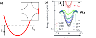
Figure 4: Definition of $\mu_{0}$: a) Cut of the electron dispersion near the antinode (region shown by the line in the inset) b)Dispersion at different temperatures obtained from ARPES experimentBi2201ARPES-1 , with $\mu_{0}$ shown. Note that the pseudogap seen in the low-temperature dispersions is clearly larger than $\mu_{0}$.

In reality, the values of $\mu_{0}$ can be smaller than the pseudogap energy and are of order of several hundred Kelvin Bi2201ARPES-1 ; Bi2201ARPES-2 ; Bi2212ARPES-1 ; Bi2212ARPES-2 . In this situation, one has to go beyond the vicinity of the FS where the spectrum cannot be linearized. Indeed, we will see that results concerning the charge orderMetSach ; Efetov2013 ; Sach2013 drastically change if the spectrum in the antinodal regions is treated more accurately. Therefore, the fermionic part of the correct SF model should contain the whole spectrum $\varepsilon\left(\mathbf{p}\right)$ of the fermions in the antinodal regions in order to enable one to consider shallow profiles of the energy spectra.

2) Following the idea of integrating out high energy degrees of freedom in a microscopic model there is no reason to neglect at the end the low-energy and -momentum part of the Coulomb interaction. In contrast, it is quite natural to treat it together with the critical mode on equal footing. This can especially be important if a static CDW is formed and the excess charges interact with each other electrostatically. In addition, the Coulomb interaction affects the competition between superconductivity and charge orders reducing the former and enhancing the latter.

The action $S$ for the extended spin fermion model capable to take into account 1) and 2) can be written in the form

$$S=S_{\mathrm{0}}+S_{\mathrm{\psi}}+S_{\mathrm{\phi}}+S_{\mathrm{c}}$$ (12)

In Eq. (12), $S_{0}$ stands for the action of non-interacting fermions (electrons)

$$S_{\mathrm{0}}=\int\chi^{\dagger}\left(X\right)\left[\partial_{\tau}+\varepsilon\left(-i\nabla_{\mathbf{r}}\right)-\mu_{0}\right]\chi\left(X\right)dX,$$ (13)

where $X=\left(\tau,\mathbf{r}\right),$ while

$$S_{\mathrm{\psi}}=\lambda\int\chi^{\dagger}\left(X\right)\vec{\sigma}\vec{\phi}\left(X\right)\chi\left(X\right)dX\mathbf{,}$$ (14)

describes the interaction of the fermions with the effective exchange field $\vec{\phi}\left(\tau,\mathbf{r}\right)$ of the antiferromagnet. In Eqs. (13, 14), $\chi$ is the anticommuting fermionic field with two spin components, $\vec{\sigma}$ is the vector of Pauli matrices, and $\tau$ is the imaginary time. The fermionic field $\chi$ has two spin components

$$\chi=\left(\begin{array}[]{c}\chi_{1}\\ \chi_{2}\end{array}\right)$$ (15)

The second term in Eq. (13) stands for the fermion energy operator, and $\mu_{0}$ is the chemical potential counted from $\varepsilon(\pi,0)$ or $\varepsilon(0,\pi)$. At the moment, we do not make any assumption about the form of the fermion operator $\varepsilon\left(-i\nabla_{\mathbf{r}}\right)$. A proper form of this operator will be chosen when making explicit calculations.

The Lagrangian $S_{\mathrm{\phi}}$ for the slow exchange field $\vec{\phi}$ is written near QCP as

$$S_{\mathrm{\phi}}=\frac{1}{2}\int\Big{[}\vec{\phi}\left(X\right)\left[\hat{D}_{0}^{-1}+\frac{g\vec{\phi}^{2}\left(X\right)}{2}\right]\vec{\phi}\left(X\right)\Big{]}dX.$$ (16)

The propagator $\hat{D}_{0}$ describes the spectrum of the antiferromagnetic paramagnons near QCP and we chose it in the form

$$\hat{D}_{0}^{-1}=-v_{s}^{-2}\frac{\partial^{2}}{\partial\tau^{2}}+2a_{0}^{-2}\Big{[}1-\cos\left[a_{0}\left(-i\mathbf{\nabla+Q}_{AF}\right)\right]\Big{]}+a.$$ (17)

where $\mathbf{Q}_{AF}=\left(\pi/a_{0},\pi/a_{0}\right)$. In Eq. (17), $v_{s}$ is the velocity of the spin waves, $a$ characterizes the distance from QCP ($a>0$ on the metallic side and $a<0$ in the AF region). We note, thatSFREV the polarization corrections will strongly affect the paramagnon dynamics at low frequencies, introducing the Landau damping term $\sim|\omega_{n}|$ into the propagator. In this Section we study the order parameter symmetry properties at the qualitative level and do not consider these. However, they are fully taken into account in the calculations presented in Section IV.2.

The last term $S_{\mathrm{c}}$ in Eq. (12) describes the Coulomb interaction between slowly fluctuating charges. We write this term in the form

$$S_{\mathrm{c}}=\frac{1}{2}\int V_{\mathrm{c}}\left(X-X^{\prime}\right)$$ (18)

$$\times\left(\chi^{\dagger}\left(X\right)\chi\left(X\right)\right)\left(\chi^{\dagger}\left(X^{\prime}\right)\chi\left(X^{\prime}\right)\right)dXdX^{\prime}.$$

As the high energies and momenta are assumed to have been integrated out, the interaction $V_{\mathrm{c}}\left(X-X^{\prime}\right)$ in Eq. (18) is a low-energy part of the screened Coulomb interaction. It slowly varies on atomic scales as a function of coordinates and times and vanishes for fast variations.

Neglecting the quartic interaction and averaging over $\vec{\phi}\left(\tau,\mathbf{r}\right)$ with the help of Eq. (16, 17) one comes to the effective fermion-fermion interaction due to exchange by the paramagnons

$$S_{\mathrm{int}}=-\frac{\lambda^{2}}{2}\int D_{0}^{-1}\left(X-X^{\prime}\right)$$ (19)

$$\times\left(\chi^{\dagger}\left(X\right)\vec{\sigma}\chi\left(X\right)\right)\left(\chi^{\dagger}\left(X^{\prime}\right)\vec{\sigma}\chi\left(X^{\prime}\right)\right)dXdX^{\prime}$$

where $X=\left(\tau,\mathbf{r}\right)$.

The total fermion-fermion interaction $S_{\mathrm{tot}}$ equals

$$S_{\mathrm{tot}}=S_{\mathrm{int}}+S_{\mathrm{c}},$$ (20)

and the partition function $Z$ for the model introduced takes the form

$$Z=\int\exp\left[-S_{\mathrm{0}}\left[\chi\right]-S_{\mathrm{tot}}\left[\chi\right]\right]D\chi.$$ (21)

Considering both charge orders and superconductivity on equal footing is convenient with the help of vectors $\Psi$ defined asEfetov2013

$$\Psi=\frac{1}{\sqrt{2}}\left(\begin{array}[]{c}\chi^{\ast}\\ i\sigma_{2}\chi\end{array}\right),\quad\Psi^{\dagger}=\frac{1}{\sqrt{2}}\left(\begin{array}[]{cc}-\chi^{t}&-\chi^{\dagger}i\sigma_{2}\end{array}\right),$$ (22)

where “$t$” stands for transposition. This is a standard Gor’kov-Nambu representation and $\chi$ is the two-component spinor, Eq. (15).

Then, one can come to an order parameter

$$Q\left(X,X^{\prime}\right)=\left\langle\Psi\left(X\right)\Psi^{\dagger}\left(X^{\prime}\right)\tau_{3}\right\rangle,$$ (23)

($\tau_{3}$ is Pauli matrix in the Gor’kov-Nambu space) containing pairings in both particle-hole and superconducting channels. Singlet pairing is most energetically favorable and in this case one can represent the order parameter in a form of a $4\times 4$ matrix

$$\mathcal{M}=I_{\sigma}\otimes\hat{M}$$ (24)

$$\hat{M}\left(X,X^{\prime}\right)=\tau_{3}\left(\hat{W}\left(X,X^{\prime}\right)+\hat{\Delta}\left(X,X^{\prime}\right)\right).$$ (25)

In Eq. (25) matrices $\hat{W}\left(X,X^{\prime}\right)$ and $\hat{\Delta}\left(X,X^{\prime}\right)$ equal,

$$\hat{W}\left(X,X^{\prime}\right)=\left(\begin{array}[]{cc}W^{\ast}\left(X,X^{\prime}\right)&0\\ 0&W\left(X,X^{\prime}\right)\end{array}\right)$$ (26)

and

$$\hat{\Delta}\left(X,X^{\prime}\right)=\left(\begin{array}[]{cc}0&\Delta^{\ast}\left(X,X^{\prime}\right)\\ -\Delta\left(X,X^{\prime}\right)&0\end{array}\right)$$ (27)

where $\Delta\left(X,X^{\prime}\right)=\Delta\left(X^{\prime},X\right)$ and $W\left(X,X^{\prime}\right)=W^{\ast}\left(X^{\prime},X\right)$ are order parameters for singlet supercoductivity and charge modulation, respectively, and $I_{\sigma}$ is the unit matrix in the spin space. We will see later that both the order parameters have d-wave symmetry.

A detailed description of the charge and superconducting orders can be performed decoupling the electron-paramagnon and Coulomb interactions with a Hubbard-Stratonovich transformation. As a result of this decoupling, one can reduce the original integral $Z$ over the fermionic fields, Eq. (21), to an integral over slowly varying in space and time matrices $Q$. Calculation of the latter integrals is carried out by finding saddle points determined by mean field equations and integrating over fluctuations near these points.

Details of this calculation are presented in Appendix B. Here we write only the mean field equations keeping the matrix form of the order parameter $Q\left(X,X^{\prime}\right)$

$$-\hat{M}\left(X,X^{\prime}\right)=\delta\left(X-X^{\prime}\right)\tau_{3}\int V_{\mathrm{c}}\left(X-X_{1}\right)$$

$$\times\mathrm{tr}\left[\tau_{3}G\left(X_{1},X_{1}\right)\right]dX_{1}-V_{\mathrm{c}}\left(X-X^{\prime}\right)\tau_{3}G\left(X,X^{\prime}\right)\tau_{3}$$

$$+3\lambda^{2}D\left(X-X^{\prime}\right)G\left(X,X^{\prime}\right),$$ (28)

where the Green’s function $G\left(X,X^{\prime}\right)$ satisfies the equation

$$\left(\hat{H}_{0}-\hat{M}\right)G\left(X,X^{\prime}\right)=-\delta\left(X-X^{\prime}\right),$$ (29)

$$\hat{H}_{0}=\partial_{\tau}-\left[\varepsilon\left(-i\tau_{3}\nabla_{\mathbf{r}}\right)-\mu_{0}\right]\tau_{3},$$ (30)

and $D$ is a propagator of critical excitations screened by electron-hole fluctuations.

The symbol $\mathrm{tr}$ stands for the trace over elements of the matrix $M$. In the absence of the Coulomb interaction $V_{\mathrm{c}}\left(X-X^{\prime}\right)$, Eqs. (28-30) correspond to those derived in Ref. Efetov2013, . If, in addition, one linearizes the spectrum near the Fermi surface the matrix $\tau_{3}$ completely drops out from Eq. (28, 29) and the system becomes degenerate with respect to superconducting and charge modulation states (matrix elements $\Delta$ and $W$). Fluctuations between these states can be strong leading to the pseudogap state Efetov2013 .

However, in the mean field approximation, the charge modulation states and superconductivity are generally not degenerate and can be considered separately. Taking the off-diagonal part of the matrix $\hat{M}\left(X,X^{\prime}\right)$ we obtain for the superconducting order parameter

$$\hat{\Delta}\left(X,X^{\prime}\right)=\frac{1}{2}\left[3\lambda^{2}D\left(X-X^{\prime}\right)+V_{\mathrm{c}}\left(X-X^{\prime}\right)\right]$$

$$\times\left[\left(\hat{H}_{0}\tau_{3}+\hat{\Delta}\right)^{-1}-\left(\hat{H}_{0}\tau_{3}-\hat{\Delta}\right)^{-1}\right]_{X,X^{\prime}}.$$ (31)

Eq. (31) has solutions for d-wave symmetry of the order parameter. The low-energy part of the Coulomb interaction $V_{\mathrm{c}}\left(X-X^{\prime}\right)$ in Eq. (31) hinders the superconductivity. At the same time, the non-linearity in the spectrum obstructs the charge modulation and one can expect a competition between these two states.

As concerns the charge modulation, we write the equation for $\hat{W}\left(X,X^{\prime}\right)$ in the form

$$\hat{W}\left(X,X^{\prime}\right)=\delta\left(X-X^{\prime}\right)\int V_{\mathrm{c}}\left(X-X_{1}\right)$$ (32)

$$\times\mathrm{tr}\left[\left(H_{0}\tau_{3}-\hat{W}\right)^{-1}\right]_{X_{1},X_{1}}dX_{1}$$

$$+\left[3\lambda^{2}D\left(X-X^{\prime}\right)-V_{\mathrm{c}}\left(X-X^{\prime}\right)\right]\left[\left(H_{0}\tau_{3}-\hat{W}\right)^{-1}\right]_{X,X^{\prime}}$$

The quadrupole density wave with the diagonal modulation MetSach ; Efetov2013 has already the d-wave symmetry and the first term in R.H.S. of Eq. (32) (Hartree-type of the contribution) vanishes in this case. At the same time, states with a charge modulations along the bonds are very sensitive to the classical part of the Coulomb interaction described by this term. The expression under the trace is the full excess charge in the unit cell and it is energetically favorable to have quadrupole-like configurations for which this term vanishes. It is the first term in R.H.S. of Eq. (32) that generally leads to the d-form factor symmetry of the charge modulation even if the latter is not directed along the diagonals of the lattice. The sign of the Fock-type of the contributions of the Coulomb interaction $V_{\mathrm{c}}\left(X-X^{\prime}\right)$ in Eq. (32) is opposite to the one in Eq. (31) and this interaction enhances the charge modulation.

Eqs. (31, 32) can be rewritten in the momentum and frequency representation and solved explicitly. Depending on the parameters, Eqs. (31, 32) allow not only solutions for superconductivity and charge modulation with a finite vector $\mathbf{Q}$ but also an intracell charge modulation with $\mathbf{Q}=0$ leading to a reconstruction of the FS. The latter corresponds to a Pomeranchuk instability and we will demonstrate in the next Section that it can be in a certain region of the parameters the strongest instability in the system. We also note that in this Section we have not considered the normal-state interaction effects, e.g. fermion self-energy and polarization effects. These effects turn out to be important and they are fully taken into account in Section IV.2.

IV Pomeranchuk instability and reconstruction of the Fermi surface.

We concentrate now on studying the charge order formation in the “hot regions” of the FS approximately connected by the antiferromagnetic wave vector $(\pi/a_{0},\pi/a_{0})$ (see Fig. 5). At the moment, we neglect the possibility of the superconducting transition. This assumption can be justified by the presence of the long range part of the Coulomb interaction in Eqs. (31, 32). We assume that it is essential only inside the hot regions, thus enhancing the charge modulation, Eq. (32), and hindering the superconductivity, Eq. (31).

It is important to emphasize that we consider the situation when eight hot spots of the traditional SF model SFREV strongly overlap due to the shallow profile of the spectrum near the antinodes and we have effectively two hot regions 1 and 2 (see Fig. 5). In order to simplify the calculations, we assume that the Coulomb interaction is large at small momenta and the Hartree contribution in Eq. (32) is very large unless the excess intra-unit-cell charge in the language of the one band model is equal to zero. The latter condition excludes any charge on the $Cu$ atoms or, in other words, the s-form factor component of the charge distribution. Moreover, the s’-component can also be neglected due to smallness of ($\cos k_{x}+\cos k_{y})$ in the antinodal region.

Therefore, we can analyze the mean field equation (32) assuming from the beginning the d-form factor symmetry of the charge modulations. Of course, the solution of Ref. Efetov2013 automatically satisfies this condition. However, we will see in this section that it is not always most energetically favorable. We proceed with seeking for solutions of Eq. (32) for arbitrary modulation vectors $\mathbf{Q}$ and find the one providing the highest transition temperature. As the interaction of electrons via paramagnons is frequency dependent, it is not possible to obtain a full analytical solution. Moreover, there one needs to modify the equation (32) to include the normal-state self energy corrections. This will be done essentially as in Ref. Efetov2013 . However, the mechanism of the charge order formation can be understood analytically considering a simplified model with a frequency and momentum independent inter-region repulsion replacing the original electron-electron interaction via paramagnons. This study is presented in the next Subsection IV.1 followed by a numerical investigation of the original SF model in Subsection IV.2.

IV.1 Simplified Model

We consider two regions of the Fermi surface surrounding the antinodes 1 and 2 in Fig. 5.

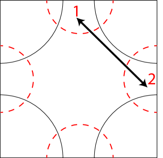
Figure 5: BZ with regions 1 and 2.

We assume a momentum and frequency independent repulsive interregion interaction and consider only d-form factor charge instabilities with an arbitrary wave vector $\mathbf{Q}$

$$W_{1}=\langle\chi_{\mathbf{p}+\mathbf{Q}/2}^{1\ast}\chi_{\mathbf{p}-\mathbf{Q}/2}^{1}\rangle=-W_{2}=-\langle\chi_{\mathbf{p}+\mathbf{Q}/2}^{2\ast}\chi_{\mathbf{p}-\mathbf{Q}/2}^{2}\rangle.$$ (33)

The form of the order parameter specified by Eq. (33) guarantees d-form factor and thus evades the on-site repulsion (first term in R.H.S. of Eq. (32)). We can solve the mean field equation (32) for $W_{\mathbf{Q}}$ for an arbitrary modulation vector $Q$.

As we are interested in the situation when the Fermi energy is not far from the $(0,\pi),(\pi,0)$ points in the electron spectrum, we expand the energy $\varepsilon^{1,2}(\mathbf{p})$ of the original Hamiltonian, Eq. (30) around them

$$\varepsilon_{p}^{1}=\alpha p_{x}^{2}-\beta p_{y}^{2}-\mu_{0},\;\varepsilon_{p}^{2}=\alpha p_{y}^{2}-\beta p_{x}^{2}-\mu_{0}$$ (34)

where $\mu_{0}$ is the Fermi energy counted from the saddle points. Moreover, we will use an averaged dispersion over $p_{y(x)}$ for region 1(2). This is justified if $\beta\ll\alpha$ (small curvature) but one can also study the qualitative effect of increasing the curvature within this approximation. Then, we write the effective dispersion in the form

$$\varepsilon_{p}^{1}=\alpha p_{x}^{2}-\mu,\quad\varepsilon_{p}^{2}=\alpha p_{y}^{2}-\mu,$$ (35)

where $\mu=\mu_{0}+\langle\beta p_{\parallel}^{2}\rangle$. We use Eq. (35) instead of Eq. (34) because this approximation simplifies the calculations but, at the same time, we do not expect an essential difference of results even when $\beta$ is of the same order as $\alpha.$ We see that the presence of the curvature leads to an effective increase of the energy $\mu$ in the antinodal regions. Having in mind applications to cuprates one can say that $\mu$ varies with the hole doping decreasing down to the point where the FS closes becoming electron-like ($\mu_{0}=0$) and further as one goes into the overdoped regime. The parameter $\alpha$ can, on the contrary, be considered as independent of the doping. The mean field Lagrangian $L_{\text{{M}}\mathrm{F}}$ for the described model can be written in the form

$$L_{\text{{M}}\mathrm{F}}=\frac{|W_{\mathbf{Q}}|^{2}}{\lambda_{0}}+\sum_{\mathbf{p},\nu=1,2}\Big{[}\chi_{\mathbf{p}}^{\nu\dagger}\left[\partial_{\tau}+\varepsilon_{i}\left(\mathbf{p}\right)\right]\chi_{\mathbf{p}}^{\nu}$$ (36)

$$+\left(-1\right)^{\nu-1}\left(W_{\mathbf{Q}}^{\ast}\chi_{\mathbf{p}+\mathbf{Q}/2}^{\nu\dagger}\chi_{\mathbf{p}-\mathbf{Q}/2}^{\nu}+W_{\mathbf{Q}}\chi_{\mathbf{p}-\mathbf{Q}/2}^{\nu\dagger}\chi_{\mathbf{p}+\mathbf{Q}/2}^{\nu}\right)\Big{]},$$

where $W_{{\bf Q}}\equiv W_{2}$.

The charge instabilities can rather easily be analyzed in this model minimizing the free energy with respect to the order parameter and linearizing the obtained equations near the transition point $T_{CO}$. Then, we come to a simple equation replacing Eq. (32) for the model considered here

$$\frac{1}{2}\sum_{\mathbf{p,}\nu=1,2}\left\{\frac{\tanh{\frac{\varepsilon_{\mathbf{p}+\mathbf{Q}/2}^{\nu}}{2T_{CO}}}-\tanh{\frac{\varepsilon_{\mathbf{p}-\mathbf{Q}/2}^{\nu}}{2T_{CO}}}}{\varepsilon_{\mathbf{p}+\mathbf{Q}/2}^{\nu}-\varepsilon_{\mathbf{p}-\mathbf{Q}/2}^{\nu}}\right\}=\frac{2}{\lambda_{0}}$$ (37)

Our goal is to find the modulation vector $\mathbf{Q}=\left(Q_{x},Q_{y}\right)$ yielding the maximal $T_{CO}$ for different values $\lambda_{0},\alpha,\mu$. First, one can notice using Eq. (35) that the L.H.S. of (37) is a sum of two identical functions with different arguments $f(Q_{x},T_{CO})+f(Q_{y},T_{CO})$, where the first term corresponds to $\nu=1$ and the second one to $\nu=2$. The temperature $T_{CO}^{max}$ is finite because $f$ is a decreasing function of $T_{CO}$ for any $Q$ for sufficiently large $T$ (one can see, making the integral in Eq. (37) dimensionless and neglecting $\sqrt{\alpha/T_{CO}}Q_{x(y)},\;\mu/T_{CO}$, that it decreases as $\sim 1/\sqrt{T_{CO}}$).

One can see now that the highest value of $T_{CO}$ will be obtained for $Q_{y},\;Q_{x}$ maximizing the L.H.S . In the case under consideration, it implies that both $f(Q_{x},T_{CO})$ and $f(Q_{y},T_{CO})$ should be maximal.

It follows then that the leading instability corresponds to $Q_{y}^{max}=Q_{x}^{max}$ and we come to the conclusion that for finite $Q_{x,y}^{max}\neq 0$ the diagonal orientation of the CDW wave vector is most favorable. This correlates with the results of the previous studyMetSach ; Efetov2013 ; Sach2013 .

However, these simple arguments do not exclude an order parameter with $Q_{y}^{max}=Q_{x}^{max}=0$. Of course, such an order parameter would no longer correspond to a CDW, as is evident from (36). Instead, the resulting phase would be characterized by a C₄-symmetry breaking deformation of the Fermi surface known in the literature as d-wave Pomeranchuk instabilityyamase2005 . As follows from Eq. (1), such a deformation leads to a redistribution of the charge density between $p_{x}$ and $p_{y}$ oxygen orbitals (see Fig. 6). An important property of this state is that it does not open a gap in the antinodal regions. As will be shown in Section V, this leaves the antinodal regions susceptible to further instabilities.

The main result of this Section is that the state with $\mathbf{Q}=0$ is indeed possible in the model considered here in a certain region of parameters. To distinguish the order parameter for this state from the one $W$ for the conventional CDW we denote it as $P$ and demonstrate that its finite values are really possible in the model considered. As we have understood, most favorable should be the state with $\mathbf{Q=}\left(Q,Q\right)$ maximizing the L.H.S. of Eq. (37).

In other words, we have to find the maximum of the integral $I\left(Q\right),$

$$I\left(Q\right)=\int\frac{dp}{2\pi}\frac{\tanh{\frac{\alpha(p+Q/2)^{2}-\mu}{2T_{CO}}}-\tanh{\frac{\alpha(p-Q/2)^{2}-\mu}{2T_{CO}}}}{2\alpha pQ},$$ (38)

as a function of $Q.$ Writing Eq. (38) we have used Eq. (35) and therefore the integrand does not contain the orthogonal momentum $p_{\perp}$. Integration over this momentum is replaced by the multiplication by a constant $\Lambda/2\pi$, where $\Lambda\ll a_{0}^{-1}$ is the size of the relevant antinodal region in the momentum space. The remaining integral over the momentum $p$ converges and we can extend the integration limits in the integral $I\left(Q\right),$ Eq. (38), to infinity. This justifies our assumption that the order parameter does not depend on the momentum. Changing the variables of the integration in Eq. (38) to $x=p\sqrt{\alpha/2T_{CO}}$ we reduce the integral $I\left(Q\right)$ to the form

$$I\left(Q\right)=\frac{\bar{I}\left(q\right)}{8\pi\sqrt{2T_{CO}\alpha}}$$ (39)

with

$$\bar{I}\left(q\right) = \int_{-\infty}^{\infty}\Big{[}\tanh{\left((x+q)^{2}-\frac{\mu}{2T_{CO}}\right)}$$

$$-\tanh{\left((x-q)^{2}-\frac{\mu}{2T_{CO}}\right)}\Big{]}\frac{dx}{qx}$$

where $q=\sqrt{\frac{\alpha}{2T_{CO}}}Q/2$.

One can clearly see from Eq. (IV.1) that the position of the maximum is governed by the dimensionless parameter

$$\kappa=\frac{\mu}{2T_{CO}},$$ (41)

where $T_{CO}$ is an increasing function of $\lambda_{0}$. Numerical integration in Eq. (IV.1) shows that there exists a critical value $\kappa_{cr}$ of the parameter $\kappa$ when the maximum shifts from finite $q$ to $q=0$. This value can be found analytically by expanding the function $\bar{I}\left(q\right),$ Eq. (IV.1), in $q$. The expansion can be written as

$$\bar{I}\left(q\right)=\bar{I}\left(0\right)-b\left(\kappa\right)q^{2},$$ (42)

where

$$\bar{I}\left(0\right)=\int_{0}^{\infty}\frac{8}{\cosh^{2}\left(x^{2}-\kappa\right)}dx$$ (43)

and fexpand

$$b\left(\kappa\right)=\frac{16}{3}\int_{0}^{\infty}\frac{\sinh(x^{2}-\kappa)}{\cosh^{3}(x^{2}-\kappa)}dx.$$ (44)

Eq. (43) shows that $\bar{I}\left(0\right)>0$ for any $\kappa$. The dependence of $b\left(\kappa\right)$ on $\kappa$ is more interesting. Numerical evaluation of the integral $b\left(\kappa\right)$ leads to the result that $b\left(\kappa\right)>0$ for $\kappa<\kappa_{cr}$ and $b\left(\kappa\right)<0$ for $\kappa>\kappa_{cr},$ where

$$\kappa_{cr}=0.55.$$ (45)

Negative values $b\left(\kappa\right)$ mean that the maximum of L.H.S. of Eq. (37) cannot be located at $Q=0$ and finite $Q$ are more favorable. This corresponds to the results of Refs. MetSach ; Efetov2013 ; Sach2013 obtained in the limit $T_{CO}\ll\mu$. Positive values of $b\left(\kappa\right)$ signal that the charge order with diagonal modulations does not appear and one comes to the state with $Q=0$. So, this state can show up when its transition temperature is higher than the distance $\mu_{0}$ of the Fermi energy from the saddle point of the spectrum.

It is interesting to note that the same value of $\kappa=\kappa_{cr}$ leads to the equality

$$\frac{df(0,\kappa_{cr})}{d\mu}=0$$ (46)

for the function $f\left(Q,\kappa\right)$ introduced below Eq. (37).

This derivative is negative for $\kappa>\kappa_{cr}$ and positive for $\kappa<\kappa_{cr}$. This implies that, provided the Pomeranchuk instability is the leading one, an increase of the hole doping will result in growing L.H.S. of (37) and, hence, decreasing the Pomeranchuk transition temperature $T_{Pom}$.

It is useful to obtain analytical expressions for the transition temperature $T_{pom}$ and the value of the order parameter $P(0)$ at zero temperature. Taking $Q=0$ in Eq. (37) and introducing the dimensionless units in the integral one obtains

$$T_{pom}=\frac{1}{8\alpha}\left(\frac{\lambda_{0}\Lambda}{4\pi^{2}}\right)^{2}\left[\int dx\frac{1}{\cosh^{2}(x^{2}-\mu/2T_{pom})}\right]^{2}$$ (47)

The integral in Eq. (47) is a slow function of $\mu/2T_{pom}$ when $\mu/2T_{pom}\sim 1$ and is approximately equal to $2$. Then, one has finally

$$T_{pom}\approx\frac{1}{2\alpha}\left(\frac{\lambda_{0}\Lambda}{4\pi^{2}}\right)^{2}$$ (48)

Note that the critical temperature $T_{pom}$ is proportional to the square of the coupling constant $\lambda_{0}$ and, in contrast to BCS-like formulas, can be quite high even for comparatively small values of $\lambda_{0}.$

To find $P(0)$ one has to first derive a self-consistency equation from Eq. (36) by taking $Q=0$. This leads to the following equation

$$\frac{1}{2}\sum_{\mathbf{p}}\left[\tanh{\frac{\varepsilon_{p}^{1}+P(T)}{2T}}-\tanh{\frac{\varepsilon_{p}^{2}-P(T)}{2T}}\right]=\frac{2P(T)}{\lambda_{0}}.$$ (49)

In the limit $T\rightarrow 0$ the hyperbolic tangent can be replaced by the sign function, and the integration over the momenta is performed assuming that $\left|P(0)\right|>\mu$. This leads to the following equation

$$\frac{\left|P(0)\right|}{\lambda_{0}}=\frac{\Lambda}{4\pi^{2}}\sqrt{\frac{\mu+\left|P(0)\right|}{\alpha}}$$ (50)

The solution of the resulting quadratic equation minimizing the free energy can be written as

$$\left|P(0)\right|\approx T_{Pom}+\sqrt{T_{Pom}^{2}+2\mu T_{Pom}}>\mu,$$ (51)

where we have used Eq. (48) for $T_{Pom}$. The inequality (51) follows from the condition $\kappa<0.55$ that guarantees that we are in the state with $Q=0$ and justifies the assumptions made when calculating the integral in Eq. (49).

The non-zero values of the order parameter $P\left(0\right)$ do not lead to a gap in the fermionic spectrum but the Fermi surface gets reconstructed and acquires a shape like one of those represented in Fig. 6.

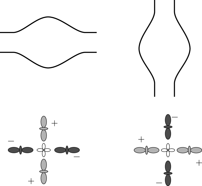
Figure 6: Pictorial representation of two possible shapes of the Fermi surface below the Pomeranchuk transition and the corresponding intra-unit-cell charge redistributions.

This leads to the breaking of the C₄ symmetry of the original charge distribution and to opposite excess charges located on $x$ and $y$ orbitals of the $O$-atoms. It is important to notice that the state is degenerate because Eq. (49) allows both $P\left(T\right)$ and $-P\left(T\right)$ solutions. As a result, two different configurations of the Fermi surface are possible (one- dimensional anisotropy along either $x$ or $y$ axis).

The results of this Subsection obtained in the framework of the simplified model demonstrate that the $\mathbf{Q}=0$ charge modulation can indeed occur in the model specified by the Lagrangian $L_{\mathrm{MF}},$ Eq. (36). In the next Subsection we consider a more realistic model of fermions interacting via antiferromagnetic paramagnons and come to similar conclusions also within that model.

IV.2 Spin-Fermion Model.

We consider the same two regions of the Fermi surface as in Fig. 5, with the single-particle spectrum given by Eq. (35). The interaction is mediated by critical antiferromagnetic paramagnons as specified in Eqs. (12-17). Limiting ourselves by consideration of the regions 1 and 2 as in Fig. 5 we reduce the model with the general action $S$, Eq. (12), to a model with the Lagrangian $L_{\mathrm{SF}}$

$$\begin{gathered}L_{\mathrm{SF}}=\sum_{\mathbf{p,}\nu=1,2}\chi_{\mathbf{p}}^{\nu\dagger}\left[\partial_{\tau}+\varepsilon_{\nu}\left(\mathbf{p}\right)\right]\chi_{\mathbf{p}}^{\nu}+\\ +\sum_{q}\vec{\varphi}_{-\mathbf{q}}(-v_{s}^{-2}\partial_{\tau}^{2}+\mathbf{q}^{2}+a)\vec{\varphi}_{\mathbf{q}}\\ +\lambda\sum_{\mathbf{p,q}}\left[\chi_{\mathbf{p+q}}^{1\dagger}\vec{\varphi}_{\mathbf{q}}\vec{\sigma}\chi_{\mathbf{p}}^{2}+\chi_{\mathbf{p+q}}^{2\dagger}\vec{\varphi}_{\mathbf{q}}\vec{\sigma}\chi_{\mathbf{p}}^{1}\right],\end{gathered}$$ (52)

Writing Eq. (52) we have omitted the Coulomb interaction. Its effect will be taken into account by assuming the d-form factor symmetry of the charge configurations. In addition, the presence of the Coulomb interaction is important to reduce the superconducting critical temperature, such that the Pomeranchuk transition temperature $T_{Pom}$ is the highest critical temperature in the model.

IV.2.1 Normal state properties.

First, we study the normal state (high temperature) properties of this model because they are different from those obtained in standard considerations in the vicinity of the Fermi surface. The Green’s functions for fermions and paramagnons have the form

$$G_{\alpha\beta}^{\nu}(i\varepsilon_{n},\mathbf{p})=\frac{\delta_{\alpha\beta}}{i\varepsilon_{n}-\varepsilon_{\nu}(\mathbf{p})-\Sigma_{\nu}(i\varepsilon_{n},\mathbf{p})},$$ (53)

$$D_{mm^{\prime}}(i\omega_{n},\mathbf{q})=-\frac{\delta_{mm^{\prime}}}{\left(\omega_{n}/v_{s}\right)^{2}+\mathbf{q}^{2}+a+\Pi(i\omega_{n},\mathbf{q})}.$$

We calculate the self-energy $\Sigma$ and polarization operator $\Pi$ using the same self-consistent approximation as in Ref. Efetov2013, represented by diagrams in Fig. 7.

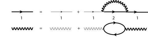
Figure 7: Feynman diagrams for fermionic and bosonic propagators illustrating the approximations used.

The self-consistent approximation used in Ref. Efetov2013, was justified by introducing an artificial small angle $\delta$ between the hot spot Fermi velocities but this is impossible for the present consideration of the antinodal regions. Fortunately, one can introduce another small parameter justifying the approximation which turns out to be quite realistic. At the moment, we neglect the momentum dependence of $\Sigma$ and $\Pi$ and justify this approximation later.

Introducing notations

$$if(\varepsilon_{n}) \equiv i\varepsilon_{n}-\Sigma(\varepsilon_{n})$$ (54)

$$\left(\lambda/v_{s}\right)^{2}\Omega(\omega_{n}) \equiv \left(\omega_{n}/v_{s}\right)^{2}+\Pi(\omega_{n}),$$ (55)

one obtains

$$f^{1(2)}(\varepsilon_{n})-\varepsilon_{n}$$

$$= -3i\lambda^{2}T\sum_{\omega_{m},\mathbf{q}}D(i\omega_{m},\mathbf{q})G^{2(1)}(\varepsilon_{n}-\omega_{m},\mathbf{p-q}),$$

$$\left(\lambda/v_{s}\right)^{2}\Omega(\omega_{n})-\left(\omega_{n}/v_{s}\right)^{2}$$

$$= 2\lambda^{2}T\sum_{\varepsilon_{n},\mathbf{p}}\Big{[}G^{1}(\mathbf{p+q},\varepsilon_{n}+\omega_{n})G^{2}(\mathbf{p},\varepsilon_{n})$$

$$+G^{2}(\mathbf{p+q},\varepsilon_{n}+\omega_{n})G^{1}(\mathbf{p},\varepsilon_{n})\Big{]}.$$

Let us now perform the integration over the momenta. First, we calculate the integral in the electron self-energy

$$\int\frac{-1}{\lambda^{2}\Omega(\varepsilon_{n}^{\prime}-\varepsilon_{n})+(\mathbf{p-p^{\prime}})^{2}+a}$$

$$\frac{1}{if(\varepsilon_{n}^{\prime})-\alpha p_{l}^{\prime 2}+\mu}\frac{d^{2}p^{\prime}}{(2\pi\hbar)^{2}},$$ (58)

where $l$ stands for $x$ or $y$. Provided the fermionic propagator is more “sharp” in the momentum space then the bosonic one, one can perform the momentum integration for the propagators independently, neglecting the term $\left(p-p^{\prime}\right)_{l}^{2}$ in the bosonic propagator. Estimating the “width” of $G$ as $\sqrt{\mu/\alpha}$ and that of $D$ as $\sqrt{a}$ we come to the condition $\mu/\alpha\ll a$. In the SF model the parameter $a$ has the meaning of the inverse square of magnetic correlation length $\xi^{-2}$. Therefore, to clarify the physical meaning of this inequality we rewrite it as

$$\mu v_{s}^{2}/\alpha\ll(v_{s}/\xi)^{2}.$$ (59)

This can be a reasonable assumption, especially taking into account that $\xi$ cannot become infinitely large at finite temperatures (see SI of Ref. Efetov2013, ). At the same time, we expect the conclusions of our study to be applicable at least qualitatively even if the inequality (59) does not hold. Performing the integration one obtains for the integral (58)

$$\frac{1}{{(2\pi)^{2}}}\frac{\pi^{2}}{\sqrt{\alpha}}$$ (60)

$$\times\sum_{\varepsilon_{n}^{\prime}}\frac{1}{\sqrt{\left(\lambda/v_{s}\right)^{2}\Omega(\varepsilon_{n}-\varepsilon_{n}^{\prime})+a}}\frac{\mathrm{sgn}(\mathrm{Re}[f(\varepsilon_{n}^{\prime})])}{\sqrt{if(\varepsilon_{n}^{\prime})+\mu}},$$

where $f(\varepsilon_{n})\equiv f^{1}(\varepsilon_{n})=f^{2}(\varepsilon_{n})$. This expression manifestly does not depend on momentum $\mathbf{p}$.

The integral over the momentum in the polarization operator $\Pi$ reads

$$\int\frac{d^{2}p}{(2\pi)^{2}}\frac{1}{if^{1}(\varepsilon_{n}+\omega_{n})-\alpha(p_{1}+q_{1})^{2}+\mu}$$

$$\times\frac{1}{if^{2}(\varepsilon_{n})-\alpha p_{2}^{2}+\mu}$$ (61)

The momenta in the fermion propagators are independent and therefore the result of the integration depends only on the incoming bosonic frequency. Then, the integral (61) equals

$$\frac{1}{{(2\pi)^{2}}}\frac{\pi^{2}}{\alpha}\sum_{\varepsilon_{n}}\frac{\mathrm{sgn}(\mathrm{Re}[f(\varepsilon_{n})])}{\sqrt{if(\varepsilon_{n})+\mu}}\frac{\mathrm{sgn}(\mathrm{Re}[f(\varepsilon_{n}+\omega_{n})])}{\sqrt{if(\varepsilon_{n}+\omega_{n})+\mu}}.$$ (62)

Introducing an energy scale

$$\Gamma=\left(\frac{\lambda^{2}v_{s}}{\sqrt{\alpha}\hbar^{2}}\right)^{2/3}$$ (63)

and dimensionless variables $\bar{f}=f/\Gamma$, $\bar{\mu}=\mu/\Gamma,$ $\bar{\omega}=\omega/\Gamma$, $\bar{\Omega}=\lambda^{2}\Omega/\Gamma^{2},$ and $\bar{a}=a\left(v_{s}/\Gamma\right)^{2}$ we can write equations corresponding to Fig. 7 in a dimensionless form

$$\bar{f}(\bar{\varepsilon}_{n})-\bar{\varepsilon}_{n}$$

$$= 0.75\bar{T}\sum_{\bar{\varepsilon}_{n}^{\prime}}\frac{1}{\sqrt{\bar{\Omega}(\bar{\varepsilon}_{n}-\bar{\varepsilon}_{n}^{\prime})+\bar{a}}}\frac{\mathrm{sgn}(\mathrm{Re}[f(\varepsilon_{n}^{\prime})])}{\sqrt{i\bar{f}(\bar{\varepsilon}_{n}^{\prime})+\bar{\mu}}},$$

$$\bar{\Omega}(\bar{\omega}_{n})-\bar{\omega}_{n}^{2}=$$

$$= -\bar{T}\sqrt{\frac{v_{s}^{2}/\alpha}{\Gamma}}\sum_{\varepsilon_{n}}\frac{\mathrm{sgn}(\mathrm{Re}[f(\varepsilon_{n})])}{\sqrt{i\bar{f}(\bar{\varepsilon}_{n})+\bar{\mu}}}\frac{\mathrm{sgn}(\mathrm{Re}[f(\varepsilon_{n}+\omega_{n})])}{\sqrt{i\bar{f}(\bar{\varepsilon}_{n}+\bar{\omega}_{n})+\bar{\mu}}}.$$

One can see that there are three dimensionless parameters $av_{s}^{2}/\Gamma^{2}$, $\mu/\Gamma$ and $\sqrt{v_{s}^{2}/\alpha\Gamma}$ that determine the behavior of the system. The last parameter is especially important because it enters the polarization operator but not the fermionic self-energy thus distinguishing between them. One can also check that the same parameter enters the renormalization of the vertex part because it contains an integral over two electron Green’s functions as in the polarization operator. Therefore, in the limit $\sqrt{v_{s}^{2}/\alpha\Gamma}\ll 1$, one comes to a conclusion that the vertex corrections can be neglected and the polarization operator might be important only at very low Matsubara frequencies due to its linear dependence on $\bar{\omega}_{n}$.

To estimate the energy scales $\mu$ and $v_{s}^{2}/\alpha$ we use experimental data for cuprates. From ARPES data on Bi-2201 presented in Refs. Bi2201ARPES-1, ; Bi2201ARPES-2, we deduce $\mu=|\varepsilon(\pi,0)-E_{F}|=25$ meV and $\alpha=\mu/p_{F}^{2}\approx 4.7\cdot 10^{3}$ meVŲ (lattice constant is $5.44$ Å). As there are no inelastic neutron scattering data available for Bi-2201, we will use the value of $v_{s}=200$ meVÅ for Bi-2212 from Ref. prb76214512, . Then, for $v_{s}^{2}/\alpha$ we obtain the value $\approx 9$ meV. As will be shown later, our scenario works well for $\bar{\mu}<0.1$ and thus, taking small values of $\sqrt{v_{s}^{2}/\alpha\Gamma}$ is reasonable.

We can also estimate the region of the magnetic correlation lengths $\xi$ where the momentum-integrated equations are quantitatively correct as $\xi<13\mathring{A}$. This corresponds to the correlation lengths of the size of several unit cells. As we consider relatively high temperatures $T\sim T^{\ast}$, the critical correlation length $\xi$ does not need to be very large in our theory. In what follows we will present the results of calculations for $\sqrt{v_{s}^{2}/\alpha\Gamma}=0.5,\;0.1$ and $\bar{a}=0.05$.

We have solved the equations (IV.2.1, IV.2.1) numerically by iterating them until the convergence is achieved. Previous treatments restricted to the vicinities of the hotspots have found $\bar{f}(\bar{\varepsilon})$ to be purely real. This corresponds to changing the fermionic dispersion $i\varepsilon_{n}\rightarrow if(\varepsilon_{n})$. In the present case we have found that the solution for $\bar{f}(\bar{\varepsilon})$ contains both real and imaginary parts. The imaginary part of $\bar{f}(\bar{\varepsilon})$ consists of two parts: a temperature-dependent constant $c(\bar{T})$, and a temperature-independent function of Matsubara frequencies $b(\bar{\varepsilon}_{n})$. The constant part enters the fermionic propagator as a renormalization of $\mu$. As we have considered the problem only in the antinodal regions, this could mean two things, namely, a temperature-dependent shift of the chemical potential of the system or a deformation of the Fermi surface. The latter effect would be possible if this constant was momentum dependent outside the regions considered here where our treatment is not applicable. However, as there is no experimental evidence for such a temperature-dependent deformation, we assume that $c(\bar{T})$ can be absorbed into the chemical potential which is fixed by the total number of particles and therefore can be considered constant at $T\ll E_{F}$.

The frequency-dependent part of $\mathrm{Im}[\bar{f}(\bar{\varepsilon})]$ is presented in Fig. 8 for several temperatures.

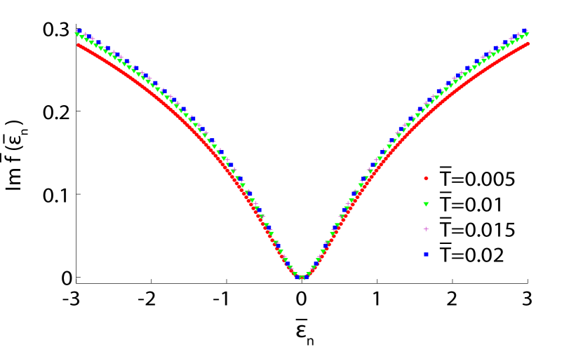
Figure 8: $\mathrm{Im}\bar{f}$ as a function of the reduced Matsubara frequency $\bar{\varepsilon}_{n}=\pi\bar{T}(2n+1)$ for different temperatures. $\bar{a}=0.05$, $\sqrt{\frac{v_{s}^{2}/\alpha}{\Gamma}}=0.5$, $\bar{\mu}=0.05$.

One can see that the function $b$ is clearly temperature-independent. To understand the physical meaning of this contribution one can perform the analytical continuation of the resulting self-energy to real frequencies $i\varepsilon_{n}\rightarrow\varepsilon$. At low frequencies $b(\bar{\varepsilon}_{n})\approx\gamma|\varepsilon_{n}|$ with $\gamma>0$. One obtains then $\delta\Sigma(i\varepsilon_{n})=\gamma|\varepsilon_{n}|\rightarrow\delta\Sigma(\varepsilon)=-i\gamma\varepsilon$. Thus, the physical meaning of this contribution is a quasiparticle damping. Note that the damping is linear in fermionic frequency in contrast to the usual $\varepsilon^{2}$ Fermi liquid dependence. This is in accord with ARPES studies of the normal state that show that the quasiparticles in the antinodal portions of the Fermi surface are strongly damped.

The results for $\Omega(\omega_{n})$ stay in line with the previous treatment Efetov2013 of the spin-fermion model. The imaginary part of this function has been found in all cases to be negligibly small (at the level of machine precision). The real part exhibits the linear Landau damping behavior at small frequencies. The constant part $\Omega(0)$ does not diverge unlike the previous treatment and therefore one can study the temperature dependence of the bosonic mass $a(T)=a+\left(\lambda/v_{s}\right)^{2}\Omega(0,T)$. However, our calculations have shown that this dependence is weak (at most, $10\%$ difference in the temperature region of interest) and so we will keep the bosonic mass constant to simplify calculations.

IV.2.2 Pomeranchuk order.

Now we will present numerical data for the emerging charge orders. First, we will compare the critical temperatures $T_{Pom}$ for the Fermi surface deformation and $T_{diag}$ for the onset of the diagonal modulation. One can argue in a similar way as in Subsection IV.1, that there exists a critical value of $\bar{\mu}$ below which the Pomeranchuk instability becomes the leading one (see Appendix C). On the other hand, for large $\bar{\mu}$ one may linearize the spectrum, which clearly leads to the diagonal CDW state Efetov2013 ; Sach2013 . One can investigate the transition from one phase to the other in more detail solving mean field equations numerically. We do not consider now the superconducting phase assuming that it has been suppressed due to the Coulomb interaction.

The equation for the Pomeranchuk d-wave symmetric order parameter $P(\varepsilon,\mathbf{p})$ can be written in the form

$$P\left(\varepsilon,\mathbf{p}\right)$$

$$= -\frac{T}{2\left(2\pi\right)^{2}}\sum_{\varepsilon^{\prime},\nu=1,2}\int\left[3\lambda^{2}D\left(\varepsilon-\varepsilon^{\prime},\mathbf{p-p}^{\prime}\right)+V_{\mathrm{c}}\left(\mathbf{p}-\mathbf{p}^{\prime}\right)\right]$$

$$\times\left(-1\right)^{\nu-1}\left[\left(if\left(\varepsilon^{\prime}\right)-\varepsilon_{\nu}\left(\mathbf{p}^{\prime}\right)+\mu+\left(-1\right)^{\nu}P\left(\varepsilon^{\prime},\mathbf{p}^{\prime}\right)\right)\right]^{-1}d\mathbf{p}^{\prime},$$

where the momentum integration is performed over the antinodal region.

The critical temperature $T_{Pom}$ can be found linearizing this equation in $P$

$$P\left(\varepsilon,\mathbf{p}\right)=\frac{T}{\left(2\pi\right)^{2}}\sum_{\varepsilon^{\prime}}\int d\mathbf{p}^{\prime}P\left(\varepsilon^{\prime},\mathbf{p}^{\prime}\right)$$ (67)

$$\times\frac{\left[3\lambda^{2}D\left(\varepsilon-\varepsilon^{\prime},\mathbf{p-p}^{\prime}\right)+V_{\mathrm{c}}\left(\mathbf{p}-\mathbf{p}^{\prime}\right)\right]}{\left[f\left(\varepsilon^{\prime}\right)+i\left(\varepsilon\left(\mathbf{p}^{\prime}\right)-\mu\right)\right]^{2}},$$

where $\varepsilon\left(\mathbf{p}\right)$ is either $\varepsilon_{1}\left(\mathbf{p}\right)$ or $\varepsilon_{2}\left(\mathbf{p}\right).$

Assuming that the order parameter does not depend on $\mathbf{p}$ one can integrate over momenta and derive the final equations for all $P\left(\varepsilon\right)$.

$$\begin{gathered}\bar{f}(\bar{\varepsilon}_{n})-\bar{\varepsilon}_{n}=0.75\bar{T}\sum_{\bar{\varepsilon}_{n}^{\prime}}\frac{1}{\sqrt{\bar{\Omega}(\bar{\varepsilon}_{n}-\bar{\varepsilon}_{n}^{\prime})+\bar{a}}}\frac{\mathrm{sgn}(\mathrm{Re}[f(\bar{\varepsilon}_{n}^{\prime})])}{2}\left[\frac{1}{\sqrt{i\bar{f}(\bar{\varepsilon}_{n}^{\prime})+\bar{\mu}+\bar{P}(\bar{\varepsilon}_{n}^{\prime})}}+\frac{1}{\sqrt{i\bar{f}(\bar{\varepsilon}_{n}^{\prime})+\bar{\mu}-\bar{P}(\bar{\varepsilon}_{n}^{\prime})}}\right]\\ \bar{P}(\bar{\varepsilon}_{n})=i\cdot 0.75\bar{T}\sum_{\bar{\varepsilon}_{n}^{\prime}}\frac{1}{\sqrt{\bar{\Omega}(\bar{\varepsilon}_{n}-\bar{\varepsilon}_{n}^{\prime})+\bar{a}}}\frac{\mathrm{sgn}(\mathrm{Re}[f(\bar{\varepsilon}_{n}^{\prime})])}{2}\left[\frac{1}{\sqrt{i\bar{f}(\bar{\varepsilon}_{n}^{\prime})+\bar{\mu}-\bar{P}(\bar{\varepsilon}_{n}^{\prime})}}-\frac{1}{\sqrt{i\bar{f}(\bar{\varepsilon}_{n}^{\prime})+\bar{\mu}+\bar{P}(\bar{\varepsilon}_{n}^{\prime})}}\right]\\ \\ \bar{\Omega}(\bar{\omega}_{n})-\bar{\omega}_{n}^{2}=-\frac{\bar{T}}{2}\sqrt{\frac{v_{s}^{2}/\alpha}{\Gamma}}\sum_{\bar{\varepsilon}_{n}}\left[\frac{\mathrm{sgn}(\mathrm{Re}[f(\varepsilon_{n})])}{\sqrt{i\bar{f}(\bar{\varepsilon}_{n})+\bar{\mu}+\bar{P}(\bar{\varepsilon}_{n})}}\frac{\mathrm{sgn}(\mathrm{Re}[f(\varepsilon_{n}+\omega_{n})])}{\sqrt{i\bar{f}(\bar{\varepsilon}_{n}+\omega_{n})+\bar{\mu}-\bar{P}(\bar{\varepsilon}_{n}+\omega_{n})}}+\right.\\ \left.\frac{\mathrm{sgn}(\mathrm{Re}[f(\varepsilon_{n})])}{\sqrt{i\bar{f}(\bar{\varepsilon}_{n})+\bar{\mu}-\bar{P}(\bar{\varepsilon}_{n})}}\frac{\mathrm{sgn}(\mathrm{Re}[f(\varepsilon_{n}+\omega_{n})])}{\sqrt{i\bar{f}(\bar{\varepsilon}_{n}+\omega_{n})+\bar{\mu}+\bar{P}(\bar{\varepsilon}_{n}+\omega_{n})}}\right].\end{gathered}$$ (68)

Equations (68) are written neglecting the Coulomb interaction $V_{\mathrm{c}}$ and are used for subsequent numerical computations.

The sum and the difference of the terms in the square brackets in the first two equations (68) guarantee the d-wave symmetry of the solution for the order parameter $P\left(\bar{\varepsilon}_{n}\right)$. Equations (68) have been written for arbitrary temperatures but, as usual, their linearized version is sufficient for calculation of the transition temperature $T_{Pom}$.

For diagonal CDW order we will restrict ourselves to calculation of the transition temperature using the linearized equation

$$\begin{gathered}\bar{W}_{diag}(\bar{\varepsilon}_{n})=\frac{0.75\bar{T}}{2}\sum_{\varepsilon_{n}^{\prime}}\frac{\bar{W}_{diag}(\bar{\varepsilon}_{n}^{\prime})}{\sqrt{\bar{\Omega}(\bar{\varepsilon}_{n}-\bar{\varepsilon_{n}^{\prime}})+\bar{a}}}\\ \times\frac{\mathrm{sgn}\left(\mathrm{Re}[f(\bar{\varepsilon}_{n}^{\prime})]\right)}{\bar{f}(\bar{\varepsilon}_{n}^{\prime})\sqrt{i\bar{f}(\bar{\varepsilon}_{n}^{\prime})+\bar{\mu}}}.\end{gathered}$$ (69)

This equation has been solved numerically by the same iteration procedure as the one used for solving Eqs. (IV.2.1, IV.2.1). The summand in the R.H.S. has been taken in a slightly non-linear form to improve the convergence (this obviously does not change the $T_{diag}$ obtained). In Fig. 9 the results for $T_{Pom}(\bar{\mu})$ and $T_{diag}(\bar{\mu})$ are presented for $\bar{a}=0.05$, $\sqrt{v_{s}^{2}/\alpha\Gamma}=0.1,\;0.5$.

The crossings of the curves give the critical values $\bar{\mu}_{cr}=0.85$ for the former case and $\bar{\mu}_{cr}=0.12$ for the latter and determine the region $T_{Pom}>T_{diag}$. In both the cases there is both a critical value of $\bar{\mu}$ and a value for which $T_{Pom}$ is maximal but, unlike the simplified model result, they do not coincide. The maximal values of $\mu/T_{Pom}$ in the case $T_{Pom}>T_{diag}$ are obtained at $\bar{\mu}_{cr}$ and are $\left(\mu/T_{Pom}\right)_{cr}=5.5$ and $\left(\mu/T_{Pom}\right)_{cr}=4.4$ for the two cases considered. These values are considerably larger the value $\approx 1.1$ obtained in the simplified model from Eqs. (41, 45). As is shown in Appendix C, this is a consequence of the renormalization of the fermionic dispersion $\bar{f}(\bar{\varepsilon}_{n})$. Assuming that $T_{Pom}$ is of the order of the pseudogap temperature but higher than the latter we conclude that the most appropriate values for $\bar{\mu}$ in the moderately underdoped regime should be around $0.03-0.06$.

This implies that $T_{Pom}$ is of the same order of magnitude as $\mu$ (probably 2-3 times smaller), which makes it quite possible that $T_{Pom}>T^{\ast}\geq T_{CDW}$. It is not surprising then that a charge modulation with a diagonal modulation vector has never been observed. According to the present results, the Pomeranchuk instability prevails changing the scenario for formation of the CDW. Formation of the diagonal modulation of Refs. MetSach, ; Efetov2013, requires considerably higher values of $\mu$ than those observed experimentally for the hole-doped cuprates.

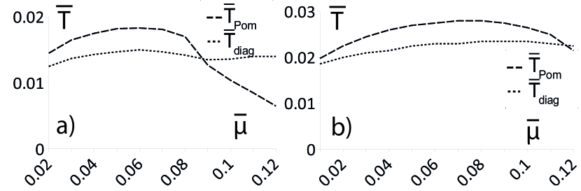
Figure 9: $\bar{T}_{Pom}(\bar{\mu})$ (dashed line) and $\bar{T}_{diag}(\bar{\mu})$ (dotted line) for $\bar{a}=0.05$, $\sqrt{\frac{v_{s}^{2}/\alpha}{\Gamma}}=0.5(a),\;0.1(b)$.

Equations (68) allow one to compute the order parameter $P\left(\bar{\varepsilon}\right)$ as a function of the reduced temperature $\bar{T}$ and frequency $\bar{\varepsilon}$. The result of the computation is presented in Figs. 10,11.

Figure 10: Dependence of real (a) and imaginary (b) parts of the Pomeranchuk order parameter $\bar{P}$ on the reduced Matsubara frequency $\bar{\varepsilon}_{n}=\pi\bar{T}(2n+1)$, $\bar{a}=0.05$, $\bar{\mu}=0.05$, $\sqrt{\frac{v_{s}^{2}/\alpha}{\Gamma}}=0.5$, $\bar{T}=0.01$.

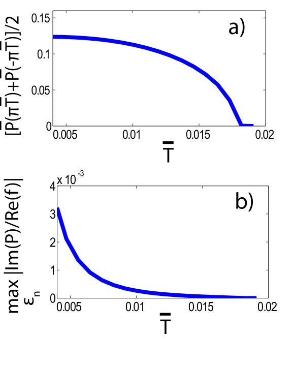
Figure 11: Dependence of the Pomeranchuk order parameter $\bar{P}$ on temperature: a) Height of the peak in the real part $0.5(\bar{P}(\pi\bar{T})+\bar{P}(-\pi\bar{T}))$ and b) Relative magnitude of the imaginary part given by $\max_{\varepsilon_{n}}\left|{\rm Im}P(\varepsilon_{n})/{\rm Re}f(\varepsilon_{n})\right|$. The model parameters are $\bar{a}=0.05$, $\sqrt{\frac{v_{s}^{2}/\alpha}{\Gamma}}=0.5$.

The non-zero values of the Pomeranchuck order parameter result in a quasi-one-dimensional shape of the Fermi surface like the one represented in Fig. 6. As a result, the bond correlations $\left\langle\chi_{i}^{\ast}\chi_{i+a_{x}}\right\rangle$ and $\left\langle\chi_{i}^{\ast}\chi_{i+a_{y}}\right\rangle$ in the SF model differ from each other. Using the correspondence between the bond correlations in the SF model and charges on the $O$ atoms on the $CuO_{2}$ lattice (SI of Ref. Efetov2013, and Appendix A) we conclude that the charges on the $O_{x}$ and $O_{y}$ orbitals are different. The resulting picture is displayed in Fig. 6.

The plot in Fig. 11 and the charge distribution in Fig. 6 are applicable at all temperatures below $T_{Pom}$ only if there are no other instabilities in this region. At the same time, the Fermi surface remains ungapped below $T_{Pom}$ and there is no reason to exclude additional phase transitions. In the next Section we will demonstrate that a d-form factor CDW with modulation along the BZ axes and d-wave superconductivity are indeed possible.

V Charge density wave and superconductivity in the model with the deformed Fermi surface.

V.1 CDW in the simplified model.

As in the previous Section, we consider first the simplified model with the constant interaction between the regions 1 and 2 in Fig. 5. Now we analyze d-form factor particle-hole instabilities at temperatures below the Pomeranchuk transition temperature, $T<$ $T_{Pom}$. As the order parameter $P\left(T\right)$ only shifts the “chemical potentials” $\mu$ in the regions 1 and 2, the equation for $T_{CO}$ (37) remains intact provided the energy spectra $\varepsilon_{p}^{1}$ and $\varepsilon_{p}^{2}$ are modified as

$$\varepsilon_{p}^{1}\rightarrow\alpha p_{x}^{2}-\mu+P(T),$$ (70)

$$\varepsilon_{p}^{2}\rightarrow\alpha p_{y}^{2}-\mu-P(T).$$

It follows then that the L.H.S. of Eq. (37) is a sum of two functions that we have already analyzed. However, the control parameters are different because instead of $\kappa\left(T\right)=\mu/2T$, one has either $\kappa_{-}=(\mu-P(T))/2T$ in the first region or $\kappa_{+}=(\mu+P(T))/2T$ in the second one. As $\left|P(T)\right|$ grows when decreasing the temperature, it is clear that below a certain temperature $T<T_{Pom}$ the susceptibility contribution from the second (from the first, if $P<0$) region will reach the maximum at a nonzero $\mathbf{Q}$ directed along $y$($x$). This happens because $\kappa_{+}\left(T\right)$ will inevitably exceed $\kappa_{cr}=0.55$ with decreasing the temperature. In the other region the situation is more subtle because, although $\mu-|P(T)|$ clearly decreases, so does the temperature $T$. It is therefore important to understand if $(\mu-|P(T)|)/2T$ can become larger than the critical value $\kappa_{cr}=0.55$ when the maximum starts to move from $\mathbf{Q}=0$ to finite $\mathbf{Q}$. Let us concentrate on the case $P\left(T\right)>0$.

An useful inequality can be derived introducing a function

$$A\left(T\right)=\left|P\left(0\right)\right|\sqrt{1-T/T_{pom}}$$ (71)

The function $A\left(T\right)$ cannot serve as a good approximation to $P\left(T\right)$ even in the vicinity of $T_{Pom}$ because the coefficient in the R.H.S. of Eq. (71) is smaller then the one given by the solution of mean field equations. For example, for the Ising model, the order parameter $P\left(T\right)=\sqrt{3}A\left(T\right)$ when $T\rightarrow T_{Pom}$. Generally, the inequality

$$P\left(T\right)\geqslant A\left(T\right)$$ (72)

holds.

The statement (72) can be proven using the fact that $P\left(0\right)=A\left(0\right)$ and $P\left(T_{Pom}\right)=A\left(T_{Pom}\right)$. As both the functions are monotonously decaying with $T$ and $\left|dP\left(T\right)/dT\right|<\left|dA\left(T\right)/dT\right|$ as $T\rightarrow 0$ (the function $P\left(T\right)$ approaches $P\left(0\right)$ exponentially in $1/T$, while $A\left(T\right)$ does it linearly in $T$), one comes the inequality (72).

This allows us to write the following inequalities

$$\frac{\mu-P(T)}{2T}\leqslant\frac{\mu-A\left(T\right)}{2T}$$ (73)

$$=\frac{\mu T/T_{Pom}+\mu(1-T/T_{pom})-A\left(T\right)}{2T}<\frac{\mu}{2T_{Pom}}.$$

The inequality in the second line of (73) follows immediately from the inequality (51) and the definition of the function $A\left(T\right)$, Eq. (71).

Inequalities (73) show that $\kappa_{-}\left(T\right)<\kappa_{Pom},$ where $\kappa_{Pom}=\mu/2T_{Pom}.$ As we are below the Pomeranchuk critical temperature $T_{Pom},$ we have $\kappa_{Pom}<\kappa_{cr}$ and, hence, $\kappa_{-}\left(T\right)<\kappa_{cr}$. With this result we come to the conclusion that the contribution of the region with the Fermi surface shrinking due to the distortion has always the maximum at the zero vector of modulation.

These simple arguments allow us to guarantee that when decreasing the temperature the Pomeranchuk transition with $\mathbf{Q}=0$ is followed by a transition into a d-form factor CDW state with the vector of modulation directed along the axes of the BZ. For $P\left(T\right)>\mu$ one comes to the Fermi surface represented in the left part of Fig. 6 and the modulation vector is directed along the y-axis, while for $P\left(T\right)<-\mu$ the picture should be turned by $90{{}^{\circ}}$. The above arguments do not exclude formation of CDW even for $-\mu<P\left(T\right)<\mu$ but due to the inequality (51) one inevitably has $\left|P\left(T\right)\right|>\mu$ at sufficiently low temperatures.

Let us now estimate the transition temperature for the CDW. We will carry out the calculations assuming $T_{CDW}\ll T_{pom}$ and checking this assumption afterwards. In this limit one can approximate the function $P(T)$ by its value $P\left(0\right)$ at zero temperature, Eq. (51). Then, the term in Eq. (37) having the maximum at the zero wave vector is proportional to $\exp{(\mu-|P(0)|)/T}\ll 1$ and therefore can be neglected. In the other term, one has an “effective Fermi energy” ${(\mu+|P(0)|)\gg T}$. In this limit the calculation of the integral in the L.H.S. of Eq. (37) is similar to a standard calculation of the corresponding integral for a CDW instability in a system with a nesting and a large Fermi energy. Then, the magnitude of the wave vector maximizing the term in Eq. (37) is given by

$$Q=2\sqrt{(\mu+\left|P(0)\right|)/\alpha},$$ (74)

which corresponds to the vector connecting the nesting points in the conventional CDW instability. As a result, one comes to the following equation

$$\frac{\Lambda}{8\pi^{2}}\int_{-\infty}^{\infty}\frac{\tanh{\frac{\alpha p^{2}+2\xi\left(p\right)}{2T_{CDW}}}-\tanh{\frac{\alpha p^{2}-2\xi\left(p\right)}{2T_{CDW}}}}{4p\sqrt{\alpha(\mu+|P(0)|)}}dp=\frac{2}{\lambda_{0}},$$ (75)

where $\xi\left(p\right)=p\sqrt{\alpha\left(\mu+P\left(0\right)\right)}.$

Changing from the variables $p$ to $\xi\left(p\right)$ one can easily calculate the integral in Eq. (75) to obtain the critical temperature $T_{CDW}$ of the transition to the CDW state

$$T_{CDW} \approx \frac{\pi}{4e^{\gamma}}(\mu+|P(0)|)\exp\left(-\frac{16\pi^{2}\sqrt{\alpha(\mu+|M(0)|)}}{\lambda\Lambda}\right)$$ (76)

$$\approx 0.44(\mu+|P(0)|)\exp\left(-4\sqrt{\frac{\mu+\left|P\left(0\right)\right|}{2T_{pom}}}\right),$$

where $\gamma\approx 0.5772$ is the Euler gamma constant and $T_{Pom}$ is determined by Eq. (48). For $T_{Pom}\sim\mu$ numerical evaluation in Eq. (76) leads to the estimate $T_{CDW}\sim 0.007\mu\ll T_{Pom}$ with a CDW wave vector magnitude $2\sqrt{(2+\sqrt{3})\mu/\alpha}\approx 1.9Q_{0}$, where $Q_{0}=2\sqrt{\mu/\alpha}$ is the vector connecting the antinodal points of the FS in case of small curvature (otherwise it is larger). As $\mu$ decreases with hole doping, so does $Q_{0}$, reproducing the qualitative behavior seen in the experimentsy123REXS-3 ; y123XRD-3 ; bi2201STM-1 . While the resulting modulation wave vector seems to be in a good agreement with experimental data bi2201STM-2 , the large difference between the temperatures $T_{Pom}\sim\mu$ and $T_{CDW}$ clearly contradicts the experimentally observed $T_{CDW}\sim 100$ K.

A possible scenario making $T_{CDW}$ closer to $T_{Pom}$ can be formulated as follows: as the Pomeranchuk distortion develops, the region where the Fermi surface shrinks can become nearly nested with a modulation vector having the same direction as in the other region. In the best case, both regions are going to have precisely the same nesting wave vector. Then, one can estimate the transition temperature by taking both contributions in Eq. (37) to be the same. This leads to $T_{CDW}\approx 0.44(\mu+|P(0)|)\exp\left(-\sqrt{2\left(\mu+|P(0)|\right)/T_{Pom}}\right)\approx 0.078\mu$, which is still too small for a quantitative agreement. Nevertheless, the qualitative scenario of a CDW transition preempted by a Fermi surface deformation transition gives a hint to the robustness of the CDW vector direction in the cuprates. In what follows, we will show that a more realistic frequency-dependent interaction of the Spin-Fermion model provides a much better quantitative estimates for $T_{CDW}$ and $Q_{CDW}$ together with a more relaxed constraint on the value of $\mu$.

Up to this point the consideration has been performed on the mean field level. However, fluctuations and inhomogeneities can manifest themselves in the proposed mean field scenario. The Pomeranchuk order parameter $P$ breaks the discrete symmetry and therefore the long-range order is not destroyed even in the strictly 2D case. Inhomogeneities, however, can be energetically profitable and proliferate in a form of domains with different signs of the order parameter. As the sign of $P$ sets the direction of the CDW, different domains will have CDWs directed in $x$ or $y$ direction depending on the sign of $P$. This indeed corresponds to recent STMBi2212STM-2 , RXSy123REXS-4 and XRDHgXRD experiments. Note that this also provides a mechanism of “masking” the C₄ symmetry breaking on the global scale alternative to the one proposed in Ref. yamase2009, . Unlike the Pomeranchuk order, CDW breaks a continuous translation symmetry and thus the transition should necessarily be smeared. Moreover, our scenario is fully compatible with the ideas of Ref. Efetov2013, , i.e. the competing orders, such as superconductivity or antiferromagnetism at lower dopings can induce an orderless pseudogap state, while lowering the ordering temperature. Thus, while it is tempting to assume $T_{CDW}\approx T^{\ast}$ in the presented scenario, fluctuations can certainly lead to $T_{CDW}<T^{\ast}$, a situation consistently observed in YBCOy123XRD-3 ; y123REXS-3 . Summarizing, the qualitative conclusions of the simplified model are:

• Provided the interaction is sufficiently strong with respect to $|\varepsilon(0,\pi)-E_{F}|,$ the Pomeranchuk instability is the leading one in the d-form factor particle-hole channel

  • There are no phase fluctuations for the Pomeranchuk order parameter and therefore the long-range order is not destroyed in 2D.

  • The order can have domain structure with different domains accommodating Fermi surface distortion either in $x$- or in $y$-directions.

• At $T_{CDW}<T_{Pom}$ a transition into a d-form factor CDW state occurs with the CDW modulation vector being directed along one of the BZ edges.

  • The direction of $\mathbf{Q}_{CDW}$ is determined by the sign of the Pomeranchuk order parameter. This implies that domains with different signs of the deformation of the Fermi surface will host CDWs with different modulation vectors.

  • The magnitude of $\mathbf{Q}_{CDW}$ depends on the magnitude of the Pomeranchuk order parameter at $T_{CDW}$ and, hence, is not universally related to $Q_{AN}$ (vector connecting adjacent antinodes) or $Q_{HS}$ (distance between hotspots or tips of the Fermi arcs). Hole doping leads to the decrease of $|\mathbf{Q}_{CDW}|$.

V.2 CDW in the Spin-Fermion model.

Now we consider formation of CDW below $T_{Pom}$ in the SF model. As the Fermi surface is not $C_{4}$ symmetric, the order parameters for purely paramagnon interaction do not necessarily satisfy in two regions 1 and 2 the equality $W_{1}=-W_{2}$ implied in the simplified model of the previous Subsection. This leads to presence of an on-site modulation (s-form factor component). However, as has been discussed in Section II, the strong on-site Coulomb repulsion suppresses on-site modulations. In principle, in order to take it into account one should solve the full equations (32).

Here we will follow a different route. In order to simplify computations, one can replace the first term in R.H.S. of Eq. (32) by the constraint

$$T\sum_{\varepsilon}\int\rho_{\mathbf{Q}}\left(\varepsilon,\mathbf{p}\right)d^{3}\mathbf{p}=0,$$ (77)

where

$$\rho_{\mathbf{Q}}\left(\varepsilon,\mathbf{p}\right)=\left\langle\chi_{\varepsilon,\mathbf{p+Q/2}}^{\dagger}\chi_{\varepsilon,\mathbf{p-Q/2}}\right\rangle$$ (78)

Equation (77) means that the total modulated charge in the elementary cell equals zero. In particular, the charge modulation on the $Cu$ atoms vanishes due to this constraint and the s-component of the charge distribution does not arise. The $O$ atoms are not explicitly present in the one-band SF model considered here. According to Appendix A the correlations $\left\langle\chi_{\mathbf{r}}^{\dagger}\chi_{\mathbf{r+a}}\right\rangle,$ where $\mathbf{a}$ is the lattice vector, determine charges on the $O$-atoms located on the bonds of $CuO_{2}$ lattice connecting the points $\mathbf{r}$ and $\mathbf{r+a}$. Within the approximations adopted in this paper the order parameter is momentum independent inside the regions 1 and 2 of Fig. 5 and therefore the charge distribution should have the d-form factor as soon as the constraint (77) is fulfilled.

For practical calculations the constraint (77) is not very convenient and we replace it by a stronger one

$$\rho_{\mathbf{Q}}^{1}\left(\varepsilon\right)+\rho_{\mathbf{Q}}^{2}\left(\varepsilon\right)=0.$$ (79)

In Eq. (79) the superscripts relate to the regions 1 and 2 in Fig. 5 but the dependence of the order parameters on the momentum is neglected inside these regions. It is easy to see that Eq. (79) leads as previously to the condition

$$W_{\mathbf{Q}}^{1}\left(\varepsilon\right)=-W_{\mathbf{Q}}^{2}\left(\varepsilon\right)$$ (80)

Note that provided the order parameter does not depend on frequency, as was the case in the simplified model, the use of the two constraints, (77) and (79) results in the same equations.

In principle, to find $T_{CDW}$ one should consider the self-consistency equations for CDW with an arbitrary wave vector $Q$ and then chose $Q$ yielding the largest transition temperature. We will obtain an estimate for $T_{CDW}$ taking $Q$ based on the results of the simplified model. $Q$ has been found to be directed along BZ axis with its magnitude given by Eq. (74). As we assume that $T_{CDW}$ can be close to $T_{Pom},$ we should accept that $P(T_{CDW})\neq P(0)$. Moreover, in the SF model the order parameter $P$ depends on the Matsubara frequency. We take these properties into account by generalizing the expression (74):

$$Q^{SF}(T)=2\sqrt{(\mu+0.5\left|P(-\pi T)+P(\pi T)\right|)/\alpha}.$$ (81)

Using this magnitude of the wave vector and taking Eq. (79) into account one obtains after momentum integration

$$\begin{gathered}\bar{W}(\bar{\varepsilon}_{n})=0.75\;i\frac{\bar{T}_{CDW}}{2}\sum_{\varepsilon_{n}^{\prime}}\frac{\mathrm{sgn}(\mathrm{Re}[f(\bar{\varepsilon}_{n}^{\prime})])}{2\sqrt{\bar{\Omega}(\bar{\varepsilon}_{n}-\bar{\varepsilon_{n}^{\prime}})+\bar{a}}}\\ \times\left[\frac{\bar{W}(\bar{\varepsilon}_{n}^{\prime})}{\left[(i\bar{f}(\bar{\varepsilon}_{n}^{\prime})+\bar{P}(\bar{\varepsilon}_{n}^{\prime})-\bar{P}(0)\right]g\left(\bar{\varepsilon}_{n}^{\prime}\right)}+\frac{\bar{W}(\bar{\varepsilon}_{n}^{\prime})}{g^{3}\left(\bar{\varepsilon}_{n}^{\prime}\right)}\right],\end{gathered}$$ (82)

where $g\left(\bar{\varepsilon}_{n}\right)=\sqrt{i\bar{f}(\bar{\varepsilon}_{n})+\bar{\mu}+\bar{P}(\bar{\varepsilon}_{n})}$ and $\bar{P}(0)=0.5\left(\bar{P}(-\pi\bar{T})+\bar{P}(\pi\bar{T})\right)$

The solution for this equations suffers from the same problem as the one for the simplified model, namely, $T_{CDW}$ is too small. For $\sqrt{v_{s}^{2}/\alpha\Gamma}=0.5$ it is at least an order of magnitude smaller then $\mu$ except for the lowest values of $\mu$ implying $T_{CDW}\sim 10-30$ $K$. Similar to what we have done for the simplified model, we would like to see if the result changes under the assumption that in the region where Fermi surface shrinks the nesting emerges. The equation for $T_{CDW}$ is then:

$$\bar{W}(\bar{\varepsilon}_{n})=0.75\;i\frac{\bar{T}_{CDW}}{2}\sum_{\varepsilon_{n}^{\prime}}\frac{\bar{W}(\bar{\varepsilon}_{n}^{\prime})}{\sqrt{\bar{\Omega}(\bar{\varepsilon}_{n}-\bar{\varepsilon_{n}^{\prime}})+\bar{a}}}$$

$$\times\frac{\mathrm{sgn}(\mathrm{Re}[f(\bar{\varepsilon}_{n}^{\prime})])}{(\left[i\bar{f}(\bar{\varepsilon}_{n}^{\prime})+\bar{P}(\bar{\varepsilon}_{n}^{\prime})-P(0)\right]g\left(\bar{\varepsilon}^{\prime}\right)}$$ (83)

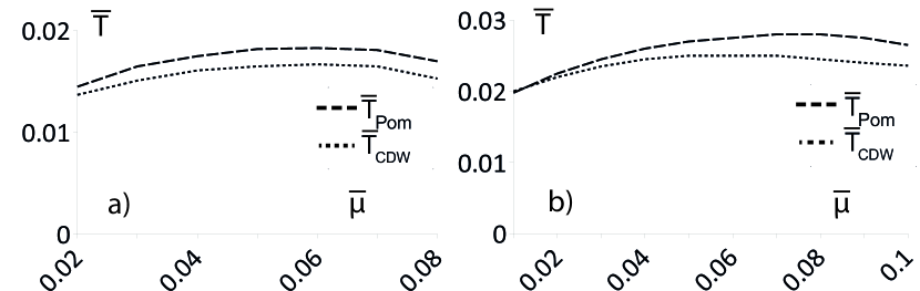
Figure 12: $T_{Pom}(\bar{\mu})$ (dashed line) and $\bar{T}_{CDW}(\bar{\mu})$ (dotted line) determined from Eq. (83) for $\bar{a}=0.05$, $\sqrt{\frac{v_{s}^{2}/\alpha}{\Gamma}}=0.5(a),\;0.1(b)$.

Results of the numerical solution are presented in Fig. 12. One can see that in this case $\bar{T}_{CDW}$ is very close to $\bar{T}_{Pom}$ making the scenario quantitatively viable. One should ask, however, if $P$ is large enough at $T_{CDW}$ to sufficiently affect the Fermi surface. In Fig. 13 the value of $0.5(P(\pi T)+P(-\pi T))$ at $T_{CDW}$ is given. One can see that the values are large enough to completely shrink the Fermi surface in one of the regions making the “nesting” assumption reasonable. From Fig. 13 one can also estimate using Eq. (81) the magnitude of $Q_{CDW}$ that turns out to be close to $1.5Q_{0}$. This also means that $Q_{CDW}$ decreases with decreasing $\bar{\mu}$, e.g. with hole doping, consistent with the experimentsy123REXS-3 ; y123XRD-3 ; bi2201STM-1 .

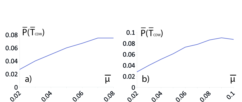
Figure 13: Value of the Pomeranchuk order parameter at the CDW transition $0.5(\bar{P}(\pi\bar{T})+\bar{P}(-\pi\bar{T}))$ for $\bar{a}=0.05$, $\sqrt{\frac{v_{s}^{2}/\alpha}{\Gamma}}=0.5(a),\;0.1(b)$.

Altogether, the results of the spin-fermion model treatment are:

• Spin-fermion model near the saddle point of the electron spectrum has a small parameter $v_{s}^{2}/\alpha\Gamma$ justifying an Eliashberg-type approximation.

• For the normal state the spin-fermion model near the saddle point yields a strong (linear) damping of antinodal quasiparticles.

• The results for the d-form factor charge ordering qualitatively agree with the simplified model from Section IV.

• Quantitatively viable results for $T_{CDW}$ can be obtained by taking into account the emerging nesting in the region with shrinking Fermi surface.

V.3 Superconductivity in the extended SF model.

Until now we have been considering charge modulations. However, superconducting phase is very important in cuprates as well as in the model considered here. It competes with the charge modulation and it is important to understand when it can win and when it cannot. Adopting Eq. (31) to the model with the two regions 1 and 2, Fig. 5, we write the equation for the superconducting order parameter in the form

$$\Delta\left(\varepsilon,\mathbf{p}\right)=\frac{T}{\left(2\pi\right)^{2}}\sum_{\varepsilon^{\prime}}\int d\mathbf{p}^{\prime}\Big{[}3\lambda^{2}D\left(\varepsilon-\varepsilon^{\prime},\mathbf{p-p}^{\prime}\right)$$

$$-V_{\mathrm{c}}\left(\mathbf{p}-\mathbf{p}^{\prime}\right)\Big{]}$$ (84)

$$\times\Delta\left(\varepsilon^{\prime},\mathbf{p}^{\prime}\right)\left[|if\left(\varepsilon^{\prime}\right)+\varepsilon\left(\mathbf{p}^{\prime}\right)-\mu|^{2}+\Delta^{2}\left(\varepsilon^{\prime},\mathbf{p}^{\prime}\right)\right]^{-1}.$$

A non-trivial solution for the superconducting $\Delta\left(\varepsilon,\mathbf{p}\right)$ appears at a critical temperature $T_{c}$ that can be found linearizing Eq. (84) in $\Delta\left(\varepsilon,\mathbf{p}\right)$

$$\Delta\left(\varepsilon,\mathbf{p}\right)=\frac{T}{\left(2\pi\right)^{2}}\sum_{\varepsilon^{\prime}}\int\Big{[}3\lambda^{2}D\left(\varepsilon-\varepsilon^{\prime},\mathbf{p-p}^{\prime}\right)$$

$$-V_{\mathrm{c}}\left(\mathbf{p}-\mathbf{p}^{\prime}\right)\Big{]}\Delta\left(\varepsilon^{\prime},\mathbf{p}^{\prime}\right)|if\left(\varepsilon^{\prime}\right)+\varepsilon\left(\mathbf{p}^{\prime}\right)-\mu|^{-2}d\mathbf{p}^{\prime}.$$

(85)

Equation (85) for the superconducting order parameter $\Delta$ differs from Eq. (67) for the Pomeranchuk order parameter $P$ by the opposite sign in front of the Coulomb interaction and by the combination $|if\left(\varepsilon^{\prime}\right)+\varepsilon\left(\mathbf{p}^{\prime}\right)-\mu|^{-2}$ instead of $\left[f\left(\varepsilon^{\prime}\right)+i\left(\varepsilon_{1}\left(\mathbf{p}^{\prime}\right)-\mu\right)\right]^{-2}$ in the integrand.

Neglecting the Coulomb interaction and performing the momentum integration one arrives at:

$$\bar{\Delta}(\varepsilon)=0.75\bar{T}\sum_{\varepsilon^{\prime}}\frac{\bar{\Delta}(\varepsilon^{\prime})}{\sqrt{\bar{\Omega}(\varepsilon-\varepsilon^{\prime})+\bar{a}}}$$

$$\frac{1}{\sqrt{\bar{\Delta}^{2}(\varepsilon^{\prime})+\mathrm{Re}[\bar{f}(\varepsilon^{\prime 2})]^{2}}}\mathrm{Re}\left[\frac{1}{\sqrt{i\bar{f}\left(\varepsilon^{\prime}\right)+\bar{\mu}}}\right].$$

The numerical solution of these equation gives consistently higher transition temperatures than for the charge orders. Actually, the $T_{c}$ obtained correspond roughly to a twice larger coupling for the SC channel (see also Eq. (69)). Qualitatively this can be explained by the fact that for a certain wave vector, only two of four hot spots in a region have nesting (and the other two are nested by the reversed wave vector), while the superconducting pairing is the same in all four hot spots. This leads to the conclusion that including Coulomb interaction is crucial for obtaining $T_{CDW}>T_{c}$. As soon as the superconducting transition is completely suppressed, one can consider the charge ordering independently, as has been done in our present study.

VI Conclusions and comparison with experiments.

Considering the spin-fermion model we have shown that contributions coming from the regions away from the Fermi surface in the antinodal regions can have an important influence on the formation of the charge order provided the dispersion is sufficiently shallow (which is motivated by the existing ARPES dataBi2201ARPES-1 ; Bi2201ARPES-2 ; Bi2212ARPES-1 ). The leading instability has been shown to be a d-wave Fermi surface distortion followed at a lower temperature by a transition into a state with a d-form factor CDW modulated with a vector directed along one of the BZ axes.

We have found that an overlap between the hot spots in the spin-fermion model leads to strongly damped quasiparticles in the normal state in accord with ARPES experiments. The transition temperatures $T_{Pom}$ and $T_{CDW}$ can be not far away from each other provided one takes into account effects of the nesting emerging on the deformed Fermi surface.

This leads to the following qualitative picture of the charge order formation:

$\bullet$ At $T_{Pom}\gtrsim T^{\ast}$ a $C_{4}$-symmetry breaking Pomeranchuk transition occurs. It manifests itself in d-form factor deformation of the Fermi surface (see Fig. 6) and a redistribution of the charge between the oxygen orbitals inside the unit cell. This can lead to formation of domains with different signs of the order parameter and different orientations of the deformed Fermi surface thus concealing the C₄-symmetry breaking for bulk probes.

$\bullet$ At $T_{CDW}<T_{Pom}$ the d-form factor CDW forms. The wave vector is directed along one of the BZ axes depending on the sign of the Pomeranchuk order parameter. The absolute value of the CDW wave vector $Q_{CDW}$ decreases with hole doping. It generally exceeds $Q_{AN}$ and should be determined self-consistently by the interaction and parameters of the Fermi surface. As a result, no universal relation between $Q_{CDW}$ and $Q_{AN}$ can be obtained.

$\bullet$ At $T_{CDW}$ the deformation of the Fermi surface should be sufficiently large in order to deform the Fermi surface to a shape with parts close to nesting like those in Fig. 6 orthogonal to the initial one. This type of the deformation can lead to quite high transition temperatures of the order of $T_{Pom}$.

The picture arising from the spin fermion model is quite general without a need of fine-tuning the parameters of the model or introducing additional components/orders.

Our findings help to explain the results of recent experiments. The Pomeranchuk deformation as a leading instability explains well the C₄ symmetry breaking at commensurate peaks in Fourier transformed STM dataBi2212STM-0 . Formation of domains with different types of the C₄-symmetry breaking is seen in STM experiments Bi2212STM-3 and can also help explaining results of the transport measurements in YBCOy123Transp-2 . The results of the measurements of Ref. y123Transp-2, show that the orientational transition preempts formation of CDW only at low dopings. However, one can imagine that, provided there are domains with different signs of the Pomeranchuk order, this transition can be seen in bulk probes only if one of the orientations is strongly preferred. It is thus possible that the C₄-symmetry breaking at higher doping is not seen in the transport measurements due to a rather small difference between the densities of the domains with the two different orientations. This may also resolve the apparent contradiction to the ARPES data Bi2201ARPES-1 ; Bi2212ARPES-1 always showing a C₄-symmetric Fermi surface.

The most important aspect of the Pomeranchuk order is that it explains the robustness of the axial d-form factor CDW in the cuprates. We also note that the organization of the CDW phase in the unidirectional domains is indeed seen in STMBi2212STM-3 and XRDy123REXS-4 ; HgXRD measurements. The coexistence of the CDW and Pomeranchuk order also allows one to resolve a seeming contradiction to results obtained in experiments on quantum oscillations seb1 ; seb2 ; sachQO . Although the unidirectional CDW leads to an open Fermi surface that does not support quantum oscillations, it has been shown in Ref. kivelson2011, that the simultaneous presence of a C₄-symmetry breaking can indeed close the Fermi surface leading to quantum oscillations in high magnetic fields.

Appendix A Hole density on oxygen sites in ZRS picture

Following Ref. ZRS, we assume that, in the limit of a weak tunneling between Cu and O atoms, doped holes entering the CuO₂ plane occupy mainly O sites forming a bound singlet state with a hole sitting on a Cu atom. In terms of the single band model derived in Ref. ZRS, , this means that the double hole occupancy of a site should be interpreted as presence of such a bound state. The wave function of this state centered around a $Cu$ hole at site $i$ with coordinate $\mathbf{R}_{i}$ is given by

$$|ZRS\rangle_{i}=\frac{|d_{i},\uparrow\rangle|\phi_{i},\downarrow\rangle-|d_{i},\downarrow\rangle|\phi_{i},\uparrow\rangle}{\sqrt{2}},$$

$$|\phi_{i},\sigma\rangle=\sum_{\alpha}a_{\alpha}^{i}|O_{\alpha},\sigma\rangle$$

$$\approx \frac{1}{2}\left(|O_{x-}^{i},\sigma\rangle-|O_{x+}^{i},\sigma\rangle+|O_{y-}^{i},\sigma\rangle-|O_{y+}^{i},\sigma\rangle\right),$$

where the index $\alpha$ enumerates all oxygen sites in the $CuO_{2}$ plane (we will use Greek indices for oxygen sites in what follows), $|d_{i},\sigma\rangle$ denotes a state with a single hole at $Cu$ site with spin $\sigma$, $O_{x-(+)}$ stands for the left (right) neighboring oxygen orbital and $O_{y-(+)}$ is the lower(upper) one. As discussed in Ref. ZRS, , the approximate expression above is not a proper state to construct an orthonormal basis because the neighboring states are not orthogonal to each other. We will employ it merely for estimating the magnitude of coefficients $a_{\alpha}^{i}$ in the final expressions, while taking into account in the derivation only general properties of the $\phi_{i}$ states.

To calculate the physical properties of the holes on oxygen sites we have to consider the action of the corresponding operators on ZRS states. We start with writing an operator destroying a hole on $O$ site $\alpha$ with spin $\sigma$:

$$\hat{p}_{\alpha,\sigma}|ZRS\rangle_{i}=\sum_{i}a_{\alpha}^{i}|d_{i},-\sigma\rangle=\sum_{i}a_{\alpha}^{i}\hat{c}_{i,\sigma}^{\dagger}|0\rangle,$$ (87)

where $\hat{c}_{i,\sigma}^{\dagger}$ is the creation operator of an electron on the site $i$ with spin $\sigma$.

In the single-band model, a ZRS on the site $i$ corresponds to an unoccupied site and the operator $\hat{p}_{\alpha,\sigma}$ effectively creates electrons in the single-band model on vacant sites. If the site was occupied, however, the action of $\hat{p}_{\alpha,\sigma}$ operator should be identically zero to avoid the double occupancy. Therefore, one should take into account this restriction by projecting out states with site $i$ occupied. These arguments lead us to the following operator form of $p_{\alpha,\sigma}$ in the single-band representation:

$$\hat{p}_{\alpha,\sigma}\equiv\frac{1}{\sqrt{2}}\sum_{i}a_{\alpha}^{i}\hat{c}_{i,\sigma}^{\dagger}\hat{\Pi}_{i}$$

$$\hat{\Pi}_{i}=(1-\hat{n}_{i,\uparrow})(1-\hat{n}_{i,\downarrow}),$$ (88)

where $\hat{n}_{i,\sigma}=\hat{c}_{i,\sigma}^{\dagger}\hat{c}_{i,\sigma}$

In order to exclude the double occupancy of an arbitrary site we use the Gutzwiller projection operator

$$\hat{P}_{GW} = \prod_{i}\hat{P}_{GW}^{i},$$ (89)

$$\hat{P}_{GW}^{i} = (1-\hat{n}_{i,\uparrow}\hat{n}_{i,\downarrow}).$$

The operator $\hat{P}_{GW}$ projects out states with the double electron occupancy, such that in the remaining wave function unoccupied states can occur only due to doping. To keep the wave function normalized we need to divide all the averages obtained by a factor $\langle\hat{P}_{GW}\rangle$. In what follows we will denote a normalized average of an operator $\hat{A}$ over a Gutzwiller projected state by $\langle\langle\hat{A}\rangle\rangle$. Now we are in position to evaluate some averages that will be useful later on

$$\langle\langle\hat{n}_{i,\sigma}\rangle\rangle=\frac{\langle\hat{P}_{GW}c_{i,\sigma}^{\dagger}c_{i,\sigma}\hat{P}_{GW}\rangle}{\langle\hat{P}_{GW}\rangle}=\frac{1-p}{2},$$

$$\hat{\Pi}_{i}=1-\hat{n}_{i,\uparrow}-\hat{n}_{i,\downarrow}+\hat{n}_{i,\uparrow}\hat{n}_{i,\downarrow}=2-\hat{n}_{i,\uparrow}-\hat{n}_{i,\downarrow}-\hat{P}_{GW}^{i},$$

$$\langle\langle\hat{\Pi}_{i}\rangle\rangle=\frac{\langle\hat{P}_{GW}\Pi_{i}\hat{P}_{GW}\rangle}{\langle\hat{P}_{GW}\rangle}=p,$$ (90)

where $p$ is the relative hole doping. We have used the fact that the normal state is an eigenstate of the total particle number operator as well as the uniformity of the normal state.

Now let us calculate the hole density on an oxygen site in the normal state:

$$n_{\alpha,\sigma}^{O}=\langle\langle\hat{p}_{\alpha,\sigma}^{\dagger}\hat{p}_{\alpha,\sigma}\rangle\rangle=\frac{1}{2}\sum_{ij}(a_{\alpha}^{i})^{\ast}a_{\alpha}^{j}\langle\langle\hat{\Pi}_{i}\hat{c}_{i,\sigma}\hat{c}_{j,\sigma}^{\dagger}\hat{\Pi}_{j}\rangle\rangle$$ (91)

$$= \frac{1}{2}\sum_{i}|a_{\alpha}^{i}|^{2}\langle\langle\hat{\Pi}_{i}(1-\hat{n}_{i,\sigma})\hat{\Pi}_{i}\rangle\rangle$$

$$+\frac{1}{2}\sum_{i\neq j}(a_{\alpha}^{i})^{\ast}a_{\alpha}^{j}\langle\langle\hat{\Pi}_{i}\hat{c}_{i,\sigma}\hat{c}_{j,\sigma}^{\dagger}\hat{\Pi}_{j}\rangle\rangle$$

$$= \frac{1}{2}\sum_{i}|a_{\alpha}^{i}|^{2}\langle\langle\hat{\Pi}_{i}\rangle\rangle+\frac{1}{2}\sum_{i\neq j}(a_{\alpha}^{i})^{\ast}a_{\alpha}^{j}\langle\langle\hat{\Pi}_{i}\hat{c}_{i,\sigma}\hat{c}_{j,\sigma}^{\dagger}\hat{\Pi}_{j}\rangle\rangle$$

$$= \frac{p}{2}\sum_{i}|a_{\alpha}^{i}|^{2}+\frac{1}{2}\sum_{i\neq j}(a_{\alpha}^{i})^{\ast}a_{\alpha}^{j}\langle\langle\hat{\Pi}_{i}\hat{c}_{i,\sigma}\hat{c}_{j,\sigma}^{\dagger}\hat{\Pi}_{j}\rangle\rangle.$$

As the system is assumed to be uniform, the mean hole density should not depend on $\alpha$. Taking into account the orthonormality conditions $\sum_{\alpha}(a_{\alpha}^{i})^{\ast}a_{\alpha}^{j}=\delta_{ij}$ one has

$$n_{\sigma}^{O}=\frac{1}{2N}\sum_{\alpha}n_{\alpha,\sigma}^{O}=\frac{p}{2}\cdot\frac{1}{2N}\sum_{i}1=\frac{p}{4}.$$ (92)

Now let us consider the case when the bond order in the single band model is present. In this case, the density of the oxygen holes changes due to the second term in Eq. (91). The unprojected mean-field state is characterized by a change of the expectation value of the bond operator $\delta\langle\hat{c}_{i,\sigma}\hat{c}_{j,\sigma}^{\dagger}\rangle\equiv\langle\hat{c}_{i,\sigma}\hat{c}_{j,\sigma}^{\dagger}\rangle_{CO}$ in the ordered phase. To calculate corresponding change in the projected average $\delta\langle\langle\hat{\Pi}_{i}\hat{c}_{i,\sigma}\hat{c}_{j,\sigma}^{\dagger}\hat{\Pi}_{j}\rangle\rangle$ we note that the operators $\hat{c}_{i,\sigma}\hat{c}_{j,\sigma}^{\dagger}$ transfer an electron from site $i$ to site $j$. As the double-occupied sites are projected out, the site $j$ should be empty, while the site $i$ is occupied by an electron. Assuming that these two conditions are uncorrelated we can reduce the influence of the projection to multiplication by projection factor $p(1-p)\approx p$ for small doping. Thus, one obtains

$$\delta n_{\alpha,\sigma}^{O}\approx p\frac{1}{2}\sum_{i\neq j}(a_{\alpha}^{i})^{\ast}a_{\alpha}^{j}\langle\hat{c}_{i,\sigma}\hat{c}_{j,\sigma}^{\dagger}\rangle_{CO},$$ (93)

where $\langle...\rangle_{CO}$ is the contribution due to charge ordering in the corresponding average. Now we rewrite $\langle\hat{c}_{i,\sigma}\hat{c}_{j,\sigma}^{\dagger}\rangle_{CO}$ in the momentum space

$$\langle\hat{c}_{i,\sigma}\hat{c}_{j,\sigma}^{\dagger}\rangle_{CO}=-e^{-i\mathbf{Q(R}_{i}\mathbf{+R}_{j}\mathbf{)}/2}\sum_{\mathbf{k}}W_{\mathbf{Q}}(k)e^{i\mathbf{Q}(\mathbf{R}_{i}-\mathbf{R}_{j})}.$$ (94)

For the pure d-form factor $\cos k_{x}-\cos k_{y}$ only the nearest-neighbor correlation functions do not vanish. Moreover, the contribution of non-nearest neighbor correlators to the hole density on the oxygen sites is suppressed because $|a_{\alpha}^{i}|$ decreases rapidly for sites not adjacent to the oxygen site $\alpha$ (e.g. $0.08$ for next nearest neighboring $Cu$ sites against $0.48$ for the nearest ones). This means that we can use the approximate expression for the ZRS wave function (A) to finally obtain

$$n_{\alpha,\sigma}^{O}\approx\frac{p}{4}+\frac{p}{8}\langle c_{i+1,\sigma}^{\dagger}c_{i,\sigma}+c_{i,\sigma}^{\dagger}c_{i+1,\sigma}\rangle_{CO},$$ (95)

where $i$ and $i+1$ are the Cu sites nearest to the oxygen site $\alpha$.

Appendix B Hubbard-Stratonovich transformation.

Using the vectors $\Psi$ and $\Psi^{\dagger}$ introduced in Eq. (22) is very convenient when the energies of the charge orders and superconductivity are close to each other. In addition to the hermitian conjugate $\Psi^{\dagger}$ of the vector $\Psi$ we introduce a “charge” conjugate field $\bar{\Psi}$ defined as

$$\bar{\Psi}=\left(C\Psi\right)^{t}\quad\text{{with}}\quad C=\left(\begin{array}[]{cc}0&i\sigma_{2}\\ -i\sigma_{2}&0\end{array}\right)_{\tau}=-\tau_{2}\sigma_{2}.$$ (96)

The matrix $C$ satisfies the relations $C^{t}C=1$ and $C=C^{t}$.

It is clear that

$$\bar{\Psi}=\Psi^{\dagger}\tau_{3}\ ,$$ (97)

where

$$\tau_{3}=\left(\begin{array}[]{cc}1&0\\ 0&-1\end{array}\right)$$

The notion of the charge conjugation is naturally extended to arbitrary matrices $M\left(X,X^{\prime}\right)$ as

$$\left(\bar{\Psi}\left(X\right)M\left(X,X^{\prime}\right)\Psi\left(X^{\prime}\right)\right)=-\left(\bar{\Psi}\left(X^{\prime}\right)\bar{M}\left(X^{\prime},X\right)\Psi\left(X\right)\right).$$ (98)

It is easy to see that

$$\bar{M}\left(X,X^{\prime}\right)=CM^{t}\left(X^{\prime},X\right)C^{t}\equiv CM^{T}\left(X,X^{\prime}\right)C^{t}\ .$$ (99)

Matrices satisfying the relation

$$\bar{M}=-M$$ (100)

are anti-selfconjugated.

Using the field $\Psi$ we rewrite Eq. (13) in the form

$$S_{\mathrm{0}}\left[\Psi\right]=\int\bar{\Psi}\left(X\right)\mathcal{H}_{0}\Psi\left(X\right)dX,$$ (101)

where the operator $\mathcal{H}_{0}=I_{\sigma}\otimes H_{0},$ $I_{\sigma}$ is the unit matrix in the spin blocks, and $H_{0}$ is determined by Eq. (30).

The term $S_{\mathrm{\psi}}$, Eq. (14), takes the form

$$S_{\mathrm{\psi}}=\lambda\int\bar{\Psi}\left(X\right)\vec{\sigma}^{t}\vec{\phi}\left(X\right)\Psi\left(X\right)dX,$$ (102)

whereas $S_{\mathrm{int}}$, Eq. (19), can be written as

$$S_{\mathrm{int}}\left[\Psi\right]=-\frac{\lambda^{2}}{2}\int D_{\mathrm{0}}\left(X-X^{\prime}\right)$$ (103)

$$\times\left(\bar{\Psi}\left(X\right)\vec{\sigma}^{t}\Psi\left(X\right)\right)\left(\bar{\Psi}\left(X^{\prime}\right)\vec{\sigma}^{t}\Psi\left(X^{\prime}\right)\right)dXdX^{\prime}$$

The Coulomb interaction $S_{\mathrm{c}}$, Eq. (18), reads now

$$S_{\mathrm{c}}=\frac{1}{2}\int V_{\mathrm{c}}\left(X-X^{\prime}\right)$$ (104)

$$\times\left(\bar{\Psi}\left(X\right)\tau_{3}\Psi\left(X\right)\right)\left(\bar{\Psi}\left(X^{\prime}\right)\tau_{3}\Psi\left(X^{\prime}\right)\right)dXdX^{\prime}$$

and the partition function $Z$ is given as before by Eq. (21).

Eqs. (20, 21, 102, 101, 103, 105) fully define the model under study.

As usualEfetov2013 , in order to reduce the integration over the fermionic fields to integration over slowly varying in space and time order parameters one has to single out slowly varying pairs of the fermionic fields. In the model under consideration, one can expect singlet superconductivity and charge orders, whereas a triplet superconductivity and spin orders are less favorable energetically.

There are $2$ equivalent possibilities to form pairs in the term $S_{\mathrm{int}}$, Eq. (103) and we write the low-energy part of $S_{\mathrm{int}}\left[\Psi\right]$ as

$$S_{\mathrm{int}}\left[\Psi\right]\rightarrow\lambda^{2}\mathrm{tr}\int D\left(X-X^{\prime}\right)$$ (105)

$$\times\vec{\sigma}^{t}\left(\Psi\left(X\right)\bar{\Psi}\left(X^{\prime}\right)\right)\vec{\sigma}^{t}\left(\Psi\left(X^{\prime}\right)\bar{\Psi}\left(X\right)\right)dXdX^{\prime}.$$

Pairing two fermionic fields $\Psi$ at equal variables $X$ would imply existence of a spin density wave but it is assumed from the beginning that the antiferromagnetic order is destroyed and one can check that additional spin structures do not appear on the metallic side. Therefore, only pairs in the brackets remain relevant in Eq. (105). They give, depending on parameters of the model, singlet superconductivity or the charge order with a certain modulation vector $\mathbf{Q}$. The value of $\mathbf{Q}$ is also determined by the parameters of the Hamiltonian. Within the standard SF model, the vector $\mathbf{Q}$ is given by the distance between the hotspots MetSach ; Efetov2013 . However, we will see that in the extended SF model introduced in the present paper, a charge modulation with $\mathbf{Q}=0$ can be more favorable in the limit of a “shallow” spectrum near the antinodes. Such a pairing leads to a reconstruction of the Fermi surface.

The Coulomb interaction is also important for obtaining this kind of the charge order. Writing relevant slow pairs in the Coulomb interaction $S_{\mathrm{c}}$, Eq. (104), one obtains two types of the contributions

$$S_{\mathrm{c}}\rightarrow\frac{1}{2}\int V_{\mathrm{c}}\left(X-X^{\prime}\right)\left(\bar{\Psi}\left(X\right)\tau_{3}\Psi\left(X\right)\right)$$

$$\times\left(\bar{\Psi}\left(X^{\prime}\right)\tau_{3}\Psi\left(X^{\prime}\right)\right)dXdX^{\prime}$$

$$-\mathrm{tr}\int V_{\mathrm{c}}\left(X-X^{\prime}\right)\tau_{3}\left(\Psi\left(X\right)\bar{\Psi}\left(X^{\prime}\right)\right)$$ (106)

$$\times\tau_{3}\left(\Psi\left(X^{\prime}\right)\bar{\Psi}\left(X\right)\right)dXdX^{\prime}.$$

The second term in Eq. (106) is analogous to the one in Eq. (105), while the first term stands for the classical part of the Coulomb interaction.

As soon as the interaction terms are written in terms of products of slow varying pairs of the fermionic fields, one can decouple the interaction integrating over slowly varying matrix fields $\mathcal{M}\left(X,X^{\prime}\right)$ having the same symmetry as the pairs $\Psi\left(X\right)\bar{\Psi}\left(X^{\prime}\right)\tau_{3}$ do. As the triplet superconducting pairing and spin density waves are less favorable we perform the decoupling using the matrices having numbers instead of spin blocks. After the decoupling is performed, the effective Lagrangian is quadratic in the fermionic fields and one can integrate out the latter.

As a result of all these standard manipulations Efetov2013 , one comes to the following expression for the partition function $Z$

$$Z = \int\exp\Big{[}\frac{1}{2}\mathrm{Tr}\ln\left(\mathcal{H}_{0}-\mathcal{M}\right)\Big{]}$$

$$\times\exp\Big{[}-\frac{1}{4}\mathrm{Tr}\left[\mathcal{M}\left(X,X^{\prime}\right)\hat{\Pi}_{\mathrm{s}}^{-1}\mathcal{M}\left(X^{\prime},X\right)\right]\Big{]}D\mathcal{Q}.$$

In Eq. (B) operator $\hat{\Pi}_{\mathrm{s}}$ acts on an arbitrary matrix function $P\left(X,X^{\prime}\right)$ as

$$\hat{\Pi}_{\mathrm{s}}P\left(X,X^{\prime}\right)=3\lambda^{2}D(X-X^{\prime})P\left(X,X^{\prime}\right)$$

$$-V_{\mathrm{c}}\left(X-X^{\prime}\right)\tau_{3}P\left(X,X^{\prime}\right)\tau_{3}$$ (108)

$$+\frac{1}{2}\delta\left(X-X^{\prime}\right)\int V_{\mathrm{c}}\left(X-X_{1}\right)\mathrm{trtr}_{\sigma}\left[\tau_{3}P\left(X_{1},X_{1}\right)\right]dX_{1},$$

where $\mathrm{tr}$ is trace in the Gor’kov-Nambu space and $\mathrm{tr}_{\sigma}$ is trace in the spin space.

Mean field equations are simply saddle point equations for the integral over $\mathcal{M}$ in Eq. (B). Minimizing the exponent in Eq. (B) we come to Eqs. (28-30) with the order parameter $M$ given by Eq. (24-30).

Appendix C Existence of $\mu_{cr}$ for SF model

We consider a linearized equation for the CDW order parameter $\bar{W}(\bar{\varepsilon}_{n})$. Assuming the CDW wave vector to be small we can decompose the R.H.S. and see at which $\bar{\mu}$ the modulation with $Q=0$ becomes favorable. We write the equation in the form

$$\bar{W}(\bar{\varepsilon}_{n})=\frac{i\cdot 0.75\bar{T}}{2}\sum_{\varepsilon_{n}^{\prime}}\frac{\bar{W}(\bar{\varepsilon}_{n})}{\sqrt{\bar{\Omega}(\bar{\varepsilon}_{n}-\bar{\varepsilon_{n}^{\prime}})+\bar{a}}}$$

$$\times\left[\frac{\mathrm{sgn}(\mathrm{Re}[f(\bar{\varepsilon}_{n}^{\prime})])}{\left(i\bar{f}(\bar{\varepsilon}_{n}^{\prime})+\bar{\mu}\right)^{3/2}}+\frac{Q^{2}}{4}\frac{\mathrm{sgn}(\mathrm{Re}[f(\bar{\varepsilon}_{n}^{\prime})])}{\left(i\bar{f}(\bar{\varepsilon}_{n}^{\prime})+\bar{\mu}\right)^{5/2}}\right].$$ (109)

In our numerical results the imaginary part of the solution has always been much smaller than the real one and concentrated at low frequencies only. For purely real order parameter one has

$$\bar{W}(\bar{\varepsilon}_{n})=\frac{-0.75\bar{T}}{2}\sum_{\varepsilon_{n}^{\prime}}\frac{\bar{W}(\bar{\varepsilon}_{n})\mathrm{sgn}(\mathrm{Re}[f(\bar{\varepsilon}_{n}^{\prime})])}{\sqrt{\bar{\Omega}(\bar{\varepsilon}_{n}-\bar{\varepsilon_{n}^{\prime}})+\bar{a}}}$$

$$\times\mathrm{Im}\left[\frac{1}{\left(i\bar{f}(\bar{\varepsilon}_{n}^{\prime})+\bar{\mu}\right)^{3/2}}+\frac{Q^{2}}{4}\frac{1}{\left(i\bar{f}(\bar{\varepsilon}_{n}^{\prime})+\bar{\mu}\right)^{5/2}}\right].$$ (110)

Then, one sees that having $Q\neq 0$ is favorable provided the imaginary parts of the two terms in the R.H.S. of Eq. (110) have the same signs. For the first term, $\left(i\bar{f}(\bar{\varepsilon}_{n}^{\prime})+\bar{\mu}\right)^{-3/2}$, the sign of the imaginary part is always $-\mathrm{sgn}(\mathrm{Re}[f(\bar{\varepsilon}_{n}^{\prime})])$ and therefore the R.H.S. of Eq. (110) is always positive at $Q=0$. As concerns the contribution coming from the second term, it can change the sign of the imaginary part. For estimation we assume that for $Q=0$ to be favorable we need the signs of imaginary parts of the two terms to be different for every frequency, even for the lowest one. Then, one has

$$\mathrm{Im}\left[\frac{1}{\left(i\bar{f}(\bar{\varepsilon}_{n}^{\prime})+\bar{\mu}_{cr}\right)^{5/2}}\right]=0.$$ (111)

Assuming $\mathrm{Im}[\bar{f}(\pi\bar{T})]$ be small we have the condition $\bar{f}(\pi\bar{T})/\bar{\mu}_{cr}=\tan(2\pi/5)\approx 3.08$. For $\bar{f}(\pi\bar{T})=\pi T$ one has $(\mu/T_{Pom})_{cr}\approx 1.02$ close to the exact result, Eq. (45) for the simplified model. However, taking into account in Eq. (111) only the lowest frequency one underestimates the value $\left(\mu/T_{Pom}\right)$. In SF model, substantially higher values $\bar{f}(\pi\bar{T})$ can also be important leading eventually to higher values of $(\mu/T_{Pom})_{cr}$. This is the reason why the numerical results for this quantity obtained in Subsection IV.2 (see Fig. (9)) are considerably higher.

References

- (1) G. Ghiringhelli, M. Le Tacon, M. Minola, S. Blanco-Canosa, C. Mazzoli, N. B. Brookes, G. M. De Luca, A. Frano, D.G. Hawthorn, F. He, T. Loew, M. Moretti Sala, D.C. Peets, M. Salluzzo, E. Schierle, R. Sutarto, G. A. Sawatzky, E. Weschke, B. Keimer, and L. Braicovich, Science 337 , 821 (2012).
- (2) S. Blanco-Canosa, A. Frano, T. Loew, Y. Lu, J. Porras, G. Ghiringhelli, M. Minola, C. Mazzoli, L. Braicovich, E. Schierle, E. Weschke, M. Le Tacon, and B. Keimer, Phys. Rev. Lett. 110, 187001 (2013).
- (3) S. Blanco-Canosa, A. Frano, E. Schierle, J. Porras, T. Loew, M. Minola, M. Bluschke, E. Weschke, B. Keimer, and M. Le Tacon, Phys. Rev. B 90, 054513 (2014).
- (4) R. Comin, R. Sutarto, E.H. da Silva Neto, L. Chauviere, R. Liang, W.N. Hardy, D.A. Bonn, F. He, G.A. Sawatzky, A. Damascelli, Science 347, 1335 (2015).
- (5) R. Comin, R. Sutarto, F. He, E.H. da Silva Neto, L. Chauviere, A. Frano, R. Liang, W.N. Hardy, D.A. Bonn, Y. Yoshida, H. Eisaki, A.J. Achkar, D.G. Hawthorn, B. Keimer, G.A. Sawatzky and A. Damascelli, Nature Mater. 14, 796 (2015).
- (6) A.J. Achkar, F. He, R. Sutarto, C. McMahon, M. Zwiebler, M. Hucker, G. D. Gu, R. Liang, D. A. Bonn, W. N. Hardy, J. Geck, D. G. Hawthorn, arXiv:1409.6787 (2014).
- (7) J. Chang, E. Blackburn, A.T. Holmes, N.B. Christensen, J. Larsen, J. Mesot, Ruixing Liang, D.A. Bonn, W.N. Hardy, A. Watenphul, M. v. Zimmermann, E.M. Forgan and S.M. Hayden, Nat. Phys. 8, 871 (2012).
- (8) E. Blackburn, J. Chang, M. Hücker, A.T. Holmes, N.B. Christensen, Ruixing Liang, D.A. Bonn, W.N. Hardy, U. Rütt, O. Gutowski, M. v. Zimmermann, E.M. Forgan, and S.M. Hayden, Phys. Rev. Lett. 110, 137004 (2013).
- (9) M. Hücker, N.B. Christensen, A.T. Holmes, E. Blackburn, E.M. Forgan, Ruixing Liang, D.A. Bonn, W.N. Hardy, O. Gutowski, M. v. Zimmermann, S. M. Hayden, and J. Chang, Phys. Rev. B 90, 054514 (2014).
- (10) E. M. Forgan, E. Blackburn, A. T. Holmes, A. Briffa, J. Chang, L. Bouchenoire, S. D. Brown, Ruixing Liang, D. Bonn, W. N. Hardy, N. B. Christensen, M. v. Zimmermann, M. Hücker, S. M. Hayden, Nat. Commun. 6, 10064 (2015).
- (11) S. Gerber, H. Jang, H. Nojiri, S. Matsuzawa, H. Yasumura, D.A. Bonn, R. Liang, W. N. Hardy, Z. Islam, A. Mehta, S. Song, M. Sikorski, D. Stefanescu, Y. Feng, S. A. Kivelson, T. P. Devereaux, Z.-X. Shen, C.-C. Kao, W.-S. Lee, D. Zhu, J.-S. Lee, Science 350, 949.
- (12) W. D. Wise, M. C. Boyer, K. Chatterjee, T. Kondo, T. Takeuchi, H. Ikuta, Y. Wang, and E. W. Hudson, Nat. Phys. 4, 696 (2008).
- (13) R. Comin, A. Frano, M.M. Yee, Y. Yoshida, H. Eisaki, E. Schierle, E. Weschke, R. Sutarto, F. He, A. Soumyanarayanan, Yang He, M. Le Tacon, I.S. Elfimov, J.E. Hoffman, G. A. Sawatzky, B. Keimer, A. Damascelli, Science 343, 390 (2014).
- (14) M. Hashimoto, G. Ghiringhelli, W.-S. Lee, G. Dellea, A. Amorese, C. Mazzoli, K. Kummer, N. B. Brookes, B. Moritz, Y. Yoshida et al., Phys. Rev. B 89, 220511 (2014).
- (15) E. H. da Silva Neto, P. Aynajian, A. Frano, R. Comin, E. Schierle, E. Weschke, A. Gyenis, J. Wen, J. Schneeloch, Z. Xu, S. Ono, G. Gu, M. Le Tacon, A. Yazdani, Science 343, 393 (2014).
- (16) M. J. Lawler, K. Fujita, J. Lee, A. R. Schmidt, Y. Kohsaka, C. K. Kim, H. Eisaki, S. Uchida, J. C. Davis, J. P. Sethna, and E.-A. Kim, Nature (London) 466 , 347 (2010).
- (17) C. V. Parker, P. Aynajian, E. H. da Silva Neto, A. Pushp, S. Ono, J. Wen, Z. Xu, G. Gu, and A. Yazdani, Nature (London) 468, 677 (2010).
- (18) K. Fujita, M. H. Hamidian, S. D. Edkins, C. K. Kim, Y. Kohsaka, M. Azuma, M. Takano, H. Takagi, H. Eisaki, S. Uchida, A. Allais, M. J. Lawler, E.-A. Kim, S. Sachdev, and J.C. Davis, Proc. Natl. Acad. Sci. U.S.A. 111, E3026 (2014).
- (19) M. H. Hamidian, S. D. Edkins, C. K. Kim, J. C. Davis, A. P. Mackenzie, H. Eisaki, S. Uchida, M. J. Lawler, E.-A. Kim, S. Sachdev, K. Fujita, Nat. Phys. 12, 150 (2016).
- (20) W. Tabis, Y. Li, M. Le Tacon, L. Braicovich, A. Kreyssig, M. Minola, G. Dellea, E. Weschke, M. J. Veit, M. Ramazanoglu, A.I. Goldman, T. Schmitt, G. Ghiringhelli, N. Barišić, M. K. Chan, C. J. Dorow, G. Yu, X. Zhao, B. Keimer, and M. Greven, Nat. Commun. 5, 5875 (2014).
- (21) G. Campi, A. Bianconi, N. Poccia, G. Bianconi, L. Barba, G. Arrighetti, D. Innocenti, J. Karpinski, N. D. Zhigadlo, S. M. Kazakov, M. Burghammer, M. v. Zimmermann, M. Sprung and A. Ricci, Nature 525, 361 (2015).
- (22) D. LeBoeuf, N. Doiron-Leyraud, J. Levallois, R. Daou, J.-B. Bonnemaison, N. E. Hussey, L. Balicas, B. J. Ramshaw, Ruixing Liang, D. A. Bonn, W. N. Hardy, S. Adachi, C. Proust, and L. Taillefer, Nature 450, 533 (2007).
- (23) N. Doiron-Leyraud, S. Lepault, O. Cyr-Choinière, B. Vignolle, G. Grissonnanche, F. Laliberté, J. Chang, N. Barišić, M. K. Chan, L. Ji, X. Zhao, Y. Li, M. Greven, C. Proust, and L.Taillefer, Phys. Rev. X 3, 021019 (2013).
- (24) N. Doiron-Leyraud, C. Proust, D. LeBoeuf, J. Levallois, J.-B. Bonnemaison, Ruixing Liang, D. A. Bonn, W. N. Hardy & L. Taillefer, Nature 447, 565 (2007).
- (25) N. Doiron-Leyraud, S. Badoux, S. René de Cotret, S. Lepault, D. LeBoeuf, F. Laliberté, E. Hassinger, B. J. Ramshaw, D. A. Bonn, W. N. Hardy, R. Liang, J.-H. Park, D. Vignolles, B. Vignolle, L. Taillefer, and C. Proust, Nat. Commun. 6, 6034 (2014).
- (26) N. Barišić, S. Badoux, M. K. Chan, C. Dorow, W. Tabis, B. Vignolle, G. Yu, J. Béard, X. Zhao, C. Proust, and M. Greven, Nat. Phys. 9, 761 (2013).
- (27) N. Harrison and S. E. Sebastian, Phys. Rev. Lett. 106, 226402 (2011).
- (28) S.E. Sebastian, N. Harrison, and G.G. Lonzarich, Rep. Prog. Phys. 75, 102501 (2012).
- (29) Andrea Allais, Debanjan Chowdhury and Subir Sachdev, Nat. Commun. 5, 5771 (2014).
- (30) T. Wu, H. Mayaffre, S. Krämer, M. Horvatić, C. Berthier, W.N. Hardy, Ruixing Liang, D.A. Bonn and M.-H. Julien, Nature 477, 191 (2011).
- (31) T. Wu, H. Mayaffre, S. Krämer, M. Horvatić, C. Berthier, W.N. Hardy, Ruixing Liang, D.A. Bonn and M.-H. Julien, Nat. Commun. 6, 6438 (2015).
- (32) D. LeBoeuf, S. Kramer, W. N. Hardy, R. Liang, D. A. Bonn, and C. Proust, Nat. Phys. 9, 79 (2013).
- (33) J. P. Hinton, J. D. Koralek, Y. M. Lu, A. Vishwanath, J. Orenstein, D. A. Bonn, W. N. Hardy, and Ruixing Liang, Phys. Rev. B 88, 060508(R) (2013).
- (34) J. M. Tranquada, AIP Conf. Proc. 1550, 114-187 (2013).
- (35) M. Hashimoto, I.M. Vishik, Rui-Hua He, T.P. Devereaux, and Z.-X. Shen, Nat. Phys. 10, 483 (2014).
- (36) A. M. Gabovich, A. I. Voitenko, T. Ekino, M. S. Li, H. Szymczak, and M. Pȩkała, Adv. Cond. Matter Phys. 2010, 681070, (2010).
- (37) M. V. Eremin and I. A. Larionov, JETP Letters 68, 611 (1998).
- (38) L. Benfatto, S Caprara, A Perali, Physica A 280, 185 (2000).
- (39) C. Castellani, C. Di Castro, and M. Grilli, Phys. Rev. Lett. 75, 4650 (1995).
- (40) A. Perali, C. Castellani, C. Di Castro, and M. Grilli, Phys. Rev. B 54, 16216 (1996).
- (41) F. Becca, M. Tarquini, M. Grilli, and C. Di Castro, Phys. Rev. B 54, 12443 (1996).
- (42) S. Caprara, C. Di Castro, M. Grilli, and D. Suppa, Phys. Rev. Lett. 95, 117004 (2005).
- (43) G. Mazza, M. Grilli, C. Di Castro, and S. Caprara, Phys. Rev. B 87, 014511 (2013).
- (44) Ar. Abanov, A. V. Chubukov, and J. Schmalian, Adv. Phys. 52, 119 (2003).
- (45) M.A. Metlitski, and S. Sachdev, Phys. Rev. B 82, 075128 (2010).
- (46) J.D. Sau, S. Sachdev, Phys. Rev. B 89, 075129 (2014).
- (47) K.B. Efetov, H. Meier, C. Pepin, Nat. Phys. 9, 442 (2013).
- (48) S. Sachdev and R. La Placa, Phys. Rev. Lett. 111,027202 (2013).
- (49) H. Meier, M. Einenkel, C. Pépin, and K. B. Efetov, Phys.Rev. B 88, 020506 (R) (2013).
- (50) M. Einenkel, H. Meier, C. Pepin, and K.B. Efetov, Phys. Rev. B 90, 054511 (2014).
- (51) J.E. Hoffman, E.W. Hudson, K.M. Lang, V. Madhavan, H. Eisaki, S. Uchida, and J.C. Davis, Science 415, 466 (2002).
- (52) M.H. Hamidian, S.D. Edkins, K. Fujita, A.P. Mackenzie, H. Eisaki, S. Uchida, M.J. Lawler, E.-A. Kim, S. Sachdev, J. C. Davis, arXiv:1508.00620.
- (53) H. Meier, C. Pepin, M. Einenkel, and K. B. Efetov, Phys. Rev. B 89, 195115 (2014).
- (54) Y. Wang, A. V. Chubukov, Phys. Rev. B 90, 035149 (2014).
- (55) C. Pépin, V. S. de Carvalho, T. Kloss, X. Montiel, Phys. Rev. B 90, 195207 (2014).
- (56) M. Punk, Phys. Rev. B 91, 115131 (2015).
- (57) J. C. Davis and D.-H. Lee, Proc. Natl. Acad. Sci. U.S.A. 110, 17623 (2013).
- (58) S. Bulut, W. A. Atkinson, and A. P. Kampf, Phys. Rev. B 88, 155132 (2013).
- (59) Y. Yamakawa and H. Kontani, Phys. Rev. Lett. 114, 257001 (2015).
- (60) W.A. Atkinson, A.P. Kampf and S. Bulut, New J. Phys. 17, 013025 (2015).
- (61) D. Chowdhury and S. Sachdev, Phys. Rev. B 90, 245136 (2014).
- (62) A. Thomson, S. Sachdev, Phys. Rev. B 91, 115142 (2015).
- (63) M. Hashimoto, R.-H. He, K. Tanaka, J.-P. Testaud, W. Meevasana, R.G. Moore, D. Lu, H. Yao, Y. Yoshida, H. Eisaki, T. P. Devereaux, Z. Hussain, and Z.-X. Shen, Nat. Phys. 6, 414 (2010).
- (64) R.-H. He, M. Hashimoto, H. Karapetyan, J. D. Koralek, J. P. Hinton, J. P. Testaud, V. Nathan, Y. Yoshida, Hong Yao, K. Tanaka, W. Meevasana, R. G. Moore, D. H. Lu, S.-K. Mo, M. Ishikado, H. Eisaki, Z. Hussain, T. P. Devereaux, S. A. Kivelson, J. Orenstein, A. Kapitulnik, Z.-X. Shen, Science 331, 1579 (2011).
- (65) A. Kaminski, S. Rosenkranz, H. M. Fretwell, M. R. Norman, M. Randeria, J. C. Campuzano, J-M. Park, Z. Z. Li, and H. Raffy, Phys. Rev. B 73, 174511 (2006).
- (66) H. Anzai, A. Ino, M. Arita, H. Namatame, M. Taniguchi, M. Ishikado, K. Fujita, S. Ishida, and S. Uchida, Nat. Com. 4, 1815 (2013).
- (67) I. J. Pomeranchuk, Sov. Phys. JETP 8, 361 (1958).
- (68) C. J. Halboth and W. Metzner, Phys. Rev. Lett. 85, 5162 (2000).
- (69) H. Yamase and Hiroshi Kohno, J. Phys. Soc. Jpn. 69, 332 (2000).
- (70) H.-Y. Kee, E. H. Kim, and C.-H. Chung, Phys. Rev. B 68, 245109 (2003).
- (71) H. Yamase, V. Oganesyan, and W. Metzner, Phys. Rev. B 72, 035114 (2005).
- (72) S. A. Kivelson, E. Fradkin and V. J. Emery, Nature 393, 550 (1998).
- (73) H. Yao, D.-H. Lee, and S.A. Kivelson, Phys. Rev. B 84, 012507 (2011).
- (74) H. Yamase, Phys. Rev. Lett. 102, 116404 (2009).
- (75) Y. B. Kim and H.-Y. Kee, J. Phys.: Condens. Matter 16, 3139 (2004).
- (76) H. Yamase and W. Metzner, Phys. Rev. B 75, 155117 (2007).
- (77) W. Metzner, D. Rohe, and S. Andergassen, Phys. Rev. Lett. 91, 066402 (2003).
- (78) H. Yamase and W. Metzner, Phys. Rev. Lett. 108, 186405 (2012).
- (79) J. Fink, N. Niicker, E. Pellegrin, H. Romberg, M. Alexander, M. Knupfer, Journal of Electron Spectroscopy and Related Phenomena 66, 395 (1994).
- (80) F. C. Zhang and T. M. Rice, Phys. Rev. B 37, 3759 (1988).
- (81) Y.-J. Chen, M. G. Jiang, C. W. Luo, J.-Y. Lin, K. H. Wu, J. M. Lee, J. M. Chen, Y. K. Kuo, J. Y. Juang, and C.-Y. Mou, Phys. Rev. B 88, 134525 (2013).
- (82) E. Kochetov, A. Ferraz, EPL, 109, 37003 (2015).
- (83) B. Fauqué, Y. Sidis, L. Capogna, A. Ivanov, K. Hradil, C. Ulrich, A. I. Rykov, B. Keimer, and P. Bourges, Phys. Rev. B 76, 214512 (2007).
- (84) Actually, expanding the function in one obtains . However, the integrating the second term by parts one comes immediately to Eq. (44).
- (85) O. Cyr-Choinire, G. Grissonnanche, S. Badoux, J. Day, D. A. Bonn, W. N. Hardy, R. Liang, N. Doiron-Leyraud, and Louis Taillefer, Phys. Rev. B 92, 224502 (2015).