How the first stars shaped the faintest gas-dominated dwarf galaxies

Abstract

Low-mass dwarf galaxies are very sensitive test-beds for theories of cosmic structure formation since their weak gravitational fields allow the effects of the relevant physical processes to clearly stand out. Up to now, no unified account exists of the sometimes seemingly conflicting properties of the faintest isolated dwarfs in and around the Local Group, such as Leo T and the recently discovered Leo P and Pisces A systems. Using new numerical simulations, we show that this serious challenge to our understanding of galaxy formation can be effectively resolved by taking into account the regulating influence of the ultraviolet radiation of the first population of stars on a dwarf’s star formation rate while otherwise staying within the standard cosmological paradigm for structure formation. These simulations produce faint, gas-dominated, star-forming dwarf galaxies that lie on the baryonic Tully-Fisher relation and that successfully reproduce a broad range of chemical, kinematical, and structural observables of real late-type dwarf galaxies. Furthermore, we stress the importance of obtaining properties of simulated galaxies in a manner as close as possible to the typically employed observational techniques.

1. INTRODUCTION

Leo P (Giovanelli et al., 2013) and Pisces A (Tollerud et al., 2015) are the latest additions to a growing list of faint, gas-rich, isolated dwarf galaxies; a list that dates back at least to the discovery of Leo T (Irwin et al., 2007). These galaxies have luminosities of only a few $10^{5}~{}\,\mathrm{L_{\odot}}$ (Ryan-Weber et al., 2008; McQuinn et al., 2013; Tollerud et al., 2015) and H i masses $3-4$ times higher than their stellar mass. Rotation velocities, derived from radio observations of the H i, are estimated at $v_{\rm rot}\sim 12.5\,\mathrm{km~{}s^{-1}}$ (Leo T: Ryan-Weber et al., 2008), $v_{\rm rot}\sim 17\,\mathrm{km~{}s^{-1}}$ (Pisces A: Tollerud et al., 2015) and $v_{\rm rot}\sim 18\,\mathrm{km~{}s^{-1}}$ (Leo P: Giovanelli et al., 2013; Bernstein-Cooper et al., 2014). The available data suggest that all three dwarfs formed stars continuously, although at a very low and highly variable rate (Clementini et al., 2012; Weisz et al., 2012; McQuinn et al., 2013, 2015).

The existence of these systems poses a strong challenge to $\Lambda$CDM, the standard model for galaxy formation and evolution: cosmological simulations predict that half of the galaxies in the nearby Universe with a circular velocity $\sim 25\,\mathrm{km~{}s^{-1}}$ are dark; these halos were never able to form stars. At a circular velocity of $\sim 15\,\mathrm{km~{}s^{-1}}$, comparable to Leo T, Leo P, and Pisces A, over 90% of all halos is predicted to be dark (Sawala et al., 2014). Indeed, supernova explosions together with the cosmic ultraviolet background (UVB), produced by the first galaxies and quasars (Efstathiou, 1992; Haardt & Madau, 1996; Faucher-Giguère et al., 2009), tend to remove the star-forming gas from low-mass dwarf galaxies. However, Tollerud et al. (2015) found that an order of magnitude difference between the observed number density of H i-detected faint dwarfs and that of corresponding dark-matter halos predicted from cosmological simulations is highly unlikely.

Clearly, these are not rare objects and many more such faint systems are likely awaiting discovery (Adams et al., 2013; Faerman et al., 2013; Adams et al., 2015; Janesh et al., 2015; Sand et al., 2015). Thus, there appears to be a disagreement between the predicted and the observed abundance of faint, gas-dominated, star-forming dwarf galaxies near the Local Group.

The process of galaxy formation is very challenging to model and the observable properties of simulated galaxies will strongly depend on the chosen set of parameters. While parameters may be tuned to get one or several galaxy properties in agreement with observations, reproducing a broad range of them is not a trivial task. Failing to reproduce one or more observable properties may be indicative that an important astrophysical process is not taken into account in the models. We thus argue that to truly reproduce realistic galaxies, one has to look at all the known observable galaxy properties. Many efforts have been made to self-consistently simulate the formation and evolution of low-mass dwarf galaxies (e.g. Governato et al., 2010; Trujillo-Gomez et al., 2011; Munshi et al., 2013; Cloet-Osselaer et al., 2014; Shen et al., 2014; Benítez-Llambay et al., 2015; Oñorbe et al., 2015; Sawala et al., 2015; Trujillo-Gomez et al., 2015; Wang et al., 2015). In this paper, we compare our simulations with as many observable properties as possible.

Here, we propose a theoretically attractive way of alleviating these tensions between simulations and observations: the energetic feedback from the first stars that formed in the universe. These so-called “population iii”, or pop iii, stars are expected to have very different properties than stars born out of even very weakly enriched gas, which are called “population ii”, or pop ii, stars. As we will show, this allows faint dwarfs with stellar masses of $M_{\star}\sim 10^{5-6}\,\mathrm{M_{\odot}}$ to grow in dark-matter halos of $M_{\rm DM}\sim 10^{9-10}\,\mathrm{M_{\odot}}$ which are massive enough to retain their cold gas reservoirs.

Below, we discuss ten numerical simulations of dwarf galaxies with different mass assembly histories in a cosmological setting with added pop iii feedback. We also ran convergence test simulations and control simulations with the same initial conditions and mass assembly histories but without pop iii feedback. The simulated dwarfs cover the entire mass range of gas-rich dwarf galaxies, allowing for a comparison with Leo T, Leo P, and Pisces A. We refer to Table 1 for an overview of the simulations. In Section 2, we discuss the code, initial conditions and analysis methods we used. The results of our simulations are shown and discussed in Section 3. Section 4 provides a short summary of this work.

2. SIMULATIONS

Our simulations were performed with the N-body/SPH-code GADGET-2 (Springel, 2005) to which we added several astrophysical ingredients, including radiative cooling, heating by the cosmic UVB and the interstellar radiation field, star formation, supernova and stellar feedback and chemical enrichment.

It is known that the standard SPH prescription suffers from several numerical issues (see e.g. Springel, 2010; Hopkins, 2015, and references therein). These are most notable in processes such as ram-pressure stripping. For our simulated galaxies, which do not experience processes where the standard SPH prescription gives significantly erroneous results, corrections to the hydrodynamical scheme will be unlikely to have a significant influence on the results.

Table 1Overview of the simulations.

(1)	(2)	(3)	(4)	(5)	(6)	(7)	(8)	(9)
Name	$M_{\mathrm{DM,tot}}$	$M_{\mathrm{prog}}$	$M_{\mathrm{res}}$	$n_{\mathrm{DM}}$	$n_{\mathrm{SPH}}$	$\epsilon_{f}$	Symbol	Notes
	$[10^{9}\,\mathrm{M}_{\odot}]$	$[10^{9}\,\mathrm{M}_{\odot}]$	$[10^{7}\,\mathrm{M}_{\odot}]$	$\times 10^{5}$	$\times 10^{5}$	$[\,\mathrm{pc}]$
DG9e9	9	1.36	5	4.5	18	6.15	$\star$
DG10e9	10	1.82	5	5	20	6.15	$\Circle$
DG12e9	12	1.88	5	6	18	6.77	$\triangleleft$
DG13e9a	13	1.86	5	6.5	6.5	9.76	$\bigtriangledown$
DG13e9b	13	2.04	5	6.5	6.5	9.76	$\bigtriangleup$	Different initial conditions
DG15e9a	15	1.82	5	7.5	7.5	9.76	$\Square$
DG15e9b	15	1.57	5	7.5	7.5	9.76	$\diamond$	Different initial conditions
DG20e9	20	3.07	10	10	10	9.76	$\pentagon$
DG50e9	50	2.98	10	10	10	13.25	$\hexagon$
DG1e11	100	7.34	20	20	20	13.25	$\varhexagon$
DG15e9b-CT	15	1.57	5	7.5	15	7.75	$\diamond$	Convergence test of DG15e9b
DG10e9-NP3	10	1.82	5	5	5	9.76	$\Circle$	DG10e9 without Pop iii feedback
DG12e9-NP3	12	1.88	5	6	6	9.76	$\triangleleft$	DG12e9 without Pop iii feedback
DG13e9b-NP3	15	2.04	5	7.5	7.5	9.76	$\bigtriangleup$	DG13e9b without Pop iii feedback

• Notes. (1): the name of the simulation, (2): total dark matter mass in the simulation, (3): the dark matter mass of the most massive progenitor, (4): the minimal progenitors mass in the merger tree, (5): number of dark matter particles, (6): number of gas particles, (7): force resolution, (8): symbol used in the figures, (9): additional notes.

2.1. Astrophysical prescriptions

As a model for star formation, a gas particle can be converted into a star particle with the same metallicity, position, and velocity if the local velocity field is converging and if the gas density is sufficiently high. With a density threshold of $100\,\mathrm{amu~{}cm^{-3}}$, star formation is restricted to cold, dense clouds of neutral gas. Each star particle represents a stellar population following the initial-mass function (IMF) of Chabrier (2003). We include thermal feedback by young, massive stars, supernovae of type ia (SNia), and type ii supernova (SNii). Young O and B stars are assumed to each inject $10^{50}$ ergs of thermal energy into the ISM while SNii and SNia explosions produce $10^{51}$ ergs per event, with an absorption efficiency of 70% by the ISM (Cloet-Osselaer et al., 2012). The delay times for SNia explosions are normally distributed with a mean of $\mu=4\,\mathrm{Gyr}$ and a dispersion $\sigma=0.8\,\mathrm{Gyr}$ (Strolger et al., 2004), cut off at $3\sigma$. SNii and SNia also enrich the ISM and, given these are the only two sources of enrichment, we only need to explicitly follow the evolution of two elements (e.g. Mg and Fe) to know the full chemical composition (De Rijcke et al., 2013). The radiative cooling and heating rate is redshift, density, temperature and metallicity dependent, taking into account self-shielding by neutral Hydrogen in high-density particles. We take into account the effect that part of the energy injected into the gas by the UVB is used to ionize the gas (Vandenbroucke et al., 2013). All these prescriptions and techniques have been used and thoroughly tested previously and a more in-depth discussion of them is available in the literature (see Valcke et al., 2008; Schroyen et al., 2011; Cloet-Osselaer et al., 2012; Schroyen et al., 2013; Verbeke et al., 2014; Cloet-Osselaer et al., 2014).

2.2. Pop iii stars

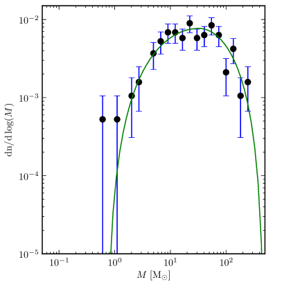
Figure 1.— Initial mass function. We use a fit (green line) through the data points (black dots) from Susa et al. (2014).

Pop iii  stars formed in the early Universe out of pristine gas. To date no pop iii stars have been directly observed and their properties are necessarily derived from theory. Simulations predict pop iii star masses in the range between 0.7 and 300 $\,\mathrm{M_{\odot}}$, with a significantly more top-heavy IMF than the Chabrier function of pop ii stars (Susa et al., 2014, Fig. 1) . Compared with a pop ii particle, a pop iii star particle injects 4 times as much thermal energy into the ISM by SNii explosions and 40 times as much by young massive stars (Heger & Woosley, 2010). 45% of the mass of a pop iii particle is returned to the ISM, with the remainder locked up in remnants, while the chemical yields of Mg and Fe are taken to be 10% of the enrichment by normal SNii explosions (Heger & Woosley, 2010; Nomoto et al., 2013). The latter is an approximation but, given the current theoretical uncertainties on pop iii yields and given the fact that a negligible fraction of the elements eventually present in the ISM comes from pop iii stars, this is without consequence. A star particle is treated as a pop iii particle if $\mathrm{[Fe/H]}<-5$.

Recently, several other advanced treatment methods of rapid stellar feedback have been suggested and shown to be important in galaxy evolution models (e.g. Stinson et al., 2013; Hopkins et al., 2014). The main difference between these and the Pop iii feedback proposed here is that the latter is inherently redshift dependent.

2.3. Initial conditions and merger trees

The mass assembly history of a simulated dwarf galaxy is modeled as a merger tree constructed using the extended Press-Schechter formalism (Bond et al., 1991; Parkinson et al., 2008) for a $\Lambda$CDM cosmology with the parameters $\Omega_{m}=0.2726$, $\Omega_{\Lambda}=0.7274$, $\Omega_{\mathrm{bar}}=0.0476$ and $\mathrm{H_{0}}=70.4\,\mathrm{km~{}s^{-1}~{}Mpc^{-1}}$, which is consistent with the results from the WMAP-9 (Hinshaw et al., 2013). We simulate the progenitors of the dwarf galaxy initially in isolation starting from $z=13.5$, and subsequently let them coalesce as prescribed by their merger tree, shown in Fig. 2. The progenitors are given an initial rotation, with both the magnitude and direction of the initial angular momentum selected randomly. Each merger event is treated as a two-body interaction with orbital parameters drawn from probability distribution functions derived from cosmological simulations (Benson, 2005).The density profile of each dark matter halo is given by:

$$\rho_{\mathrm{DM}}=\frac{\rho_{0}}{(r/r_{s})^{\alpha}(1+r/r_{s})^{4-2\alpha}},$$ (1)

with $r_{s}$ the scale length, defined as the radius where the logarithmic slope of the density profile is $-2$. The values for $\alpha$ and $r_{s}$ are drawn from cosmologically motivated mass and redshift dependent probability distribution functions (Cen et al., 2004). Although similar generalizations of the NFW profile (Navarro et al., 1996) exist (Dutton & Macciò, 2014; Klypin et al., 2014), the profiles used here have the advantage of being derived for high redshifts and down to halo masses of $M\sim 10^{6.5}M_{\odot}$. Furthermore, the density profile is significantly influenced by stellar feedback and protogalaxy mergers, so we argue that the initial density profile has little influence on the galaxy properties at $z=0$. The initial density of the gas is given by a pseudo-isothermal profile (Revaz et al., 2009):

$$\rho_{g}(r)=\frac{\rho_{0}}{1+r^{2}/r^{2}_{g}},$$ (2)

with $\rho_{0}$ the central gas density and $r_{g}$ the scale length, determined in the same way as in Schroyen et al. (2013). Initially, there are no stars present in the simulation.

We do not explicitly include accretion in the simulations, however, the simulated galaxies are surrounded by a very extended diffuse gas halo which does allow for smooth gas accretion implicitly in a self-consistent way. Similarly, the galaxies are embedded in an extended dark matter halo, which allows for growth of the dark matter halo through accretion.

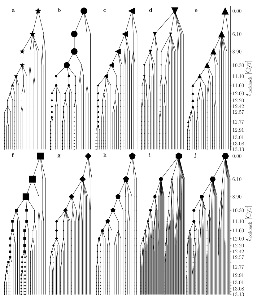
Figure 2.— Merger trees of the simulations. (a) DG9e9, (b) DG10e9, (c) DG12e9, (d) DG13e9L, (e) DG13e9E, (f) DG15e9L, (g) DG15e9E, (h) DG20e9, (i) DG50e9 and (j) DG1e11, and their respective re-simulations without pop iii  stars and the convergence test. The size of the marker is indicative of the total mass of a halo at the corresponding lookback time.

2.4. Resolution and convergence test

All but two simulations were run with the mass of the dark matter particles fixed at $m_{\mathrm{DM}}=2\times 10^{4}\,\mathrm{M_{\odot}}$, except for DG50e9 and DG1e11 with $m_{\mathrm{DM}}=5\times 10^{4}~{}M_{\odot}$. In most simulations, the mass of the gas particles was simply scaled according to the assumed baryonic to dark-matter density ratio: $\Omega_{\mathrm{bar}}/\Omega_{\mathrm{DM}}=0.2115$. Exceptions to this are DG10e9, DG12e9 and DG15e9b-CT, in which the gas resolution was increased respectively with a factor of 4, 3 and 2. In the latter, this was done as a convergence test to ensure that our results do not change depending on the resolution. As can be seen (Figs. 3$-$10), DG15e9b-CT does not differ significantly from DG15e9b and any changes can be attributed to the stochastic nature of star formation, showing that the models are sufficiently converged. In DG10e9 and DG12e9, the resolution was increased because of the low star formation efficiency in low mass halos. The force resolution of each simulation is fixed by the mass of the gas particles and the star formation criteria: the softening length is the same as the smoothing length of a gas particle that satisfies the density threshold. These are given in column 7 in Table 1. The softening length is the same for all the baryonic and dark matter particles.

2.5. Analysis

The post-processing analysis of the simulations was performed with our own publicly available software package HYPLOT. For this analysis, we adopted the strategy of staying as close as possible to the strategies adopted by observational astronomers. The comparison between properties obtained in this manner and those obtained in a way that is typically done by theorists, will be presented in an upcoming paper (Vandenbroucke et al. 2015, in preparation). The absolute magnitudes were determined by fitting an exponential function to a simulated galaxy’s surface brightness profiles out to $R_{30}$, the point where the surface brightness drops to $30\,\mathrm{mag~{}arcsec^{-2}}$, and extrapolating it to infinity to estimate the total luminosity. The V-band half-light radius $R_{e}$ was determined from this fitted profile. The stellar mass $M_{\star}$ is estimated from the V and I-band luminosities (Bell & de Jong, 2001). The neutral gas mass $M_{\mathrm{HI}}$ is determined by a straightforward summation of the masses of the gas particles multiplied with their neutral fraction. The UVB ionizes the outer, low-density regions of the ISM, limiting the H i to the more central, dense parts of the ISM of a simulated dwarf galaxy. The total baryonic mass is $M_{\mathrm{bar}}=M_{\star}+M_{\mathrm{gas,atomic}}$, with the atomic gas mass corrected for the Helium fraction: $M_{\mathrm{gas,atomic}}=M_{\mathrm{HI}}/(1-\mathrm{Y}_{\mathrm{He}})$ (with the primordial Helium abundance $\mathrm{Y}_{\mathrm{He}}=0.25$). In order to produce an “observational” estimate for the circular velocity $v_{c}$, we fitted a gaussian to a mock H i spectrum of the galaxy viewed edge-on and adopted $v_{c}=W_{20}/2$, with $W_{20}$ the full width at 20% of the maximum of this gaussian. The cumulative star formation histories (CSFH) were determined from the birth times and masses of the stellar particles within a certain radius. These CSFHs, like the observed ones, thus do not take mass loss by SNe into account. Using stellar evolution tracks for pop ii  stars (Bertelli et al., 2008, 2009) and for pop iii  stars (Marigo et al., 2001), the number of RGB stars within a given star particle can be calculated. Thus, the mean Iron abundance, $\mathrm{\langle[Fe/H]\rangle}$, can be calculated via a sum over all stellar particles weighted by the number of RGB stars in each particle. This mimics the procedure actually followed for real dwarfs (Kirby et al., 2013). For the gas, we computed the Oxygen abundance of dense gas, with each gas particle weighted by its ionized fraction. This is a measure for the metallicity of the ionized gas around star-forming regions. The SFR and atomic gas density, required for the Kennicutt-Schmidt relation, was determined within an aperture with a radius of $200\,\mathrm{pc}$ around the galaxy center. The 1D stellar velocity dispersion $\sigma_{\star}$ is measured along a line-of-sight through the galaxy, viewed edge-on, within an aperture of 1 half-light radii around the galaxy center. The solar logarithmic mass-fraction abundance of Iron is assumed to be $\mathrm{Fe/H}_{\odot}=-2.756$ and the Magnesium to Iron ratio is $\mathrm{Mg/Fe}_{\odot}=-0.261$ (Asplund et al., 2009). The virial radius $R_{{\rm halo}}$ of a dark matter halo is the radius wherin the average density equals 200 times the mean density of the universe ($\rho_{\mathrm{Univ}}=9.47\times 10^{-30}\,\mathrm{g~{}cm^{-3}}$), while the virial mass $M_{{\rm halo}}$ is the total dark matter mass within $R_{{\rm halo}}$: $M_{{\rm halo}}=\frac{4\pi}{3}200\rho_{\mathrm{Univ}}R_{{\rm halo}}^{3}$.

3. RESULTS

In what follows, all simulated galaxy properties have been calculated at the present epoch, unless explictly stated otherwise, to enable a comparison with dwarf galaxies observed in the nearby Universe. Some of the properties of the simulations at $z=0$ are given in Table 2.

Table 2Properties of the simulations at $z=0$

(1)	(2)	(3)	(4)	(5)	(6)	(7)	(8)	(9)	(10)	(11)	(12)	(13)	(14)	(15)	(16)	(17)
Name	$M_{\mathrm{*}}$	$M_{\mathrm{HI}}$	$M_{\mathrm{halo}}$	$M_{0.3}$	$M_{\mathrm{half}}$	$M_{V}$	$B-V$	$V-I$	$\mu_{0,V}$	$R_{e}$	$R_{30,V}$	$\mathrm{SFR}$	$v_{c}$	$\sigma_{*}$	$\mathrm{\langle[Fe/H]\rangle_{RGB}}$	$12+\log(\mathrm{O/H})$
	$10^{6}\,\mathrm{M}_{\odot}$	$10^{6}\,\mathrm{M}_{\odot}$	$10^{9}\,\mathrm{M}_{\odot}$	$10^{7}\,\mathrm{M_{\odot}}$	$10^{7}\,\mathrm{M_{\odot}}$	$\,\mathrm{mag}$	$\,\mathrm{mag}$	$\,\mathrm{mag}$	$\,\mathrm{mag/arcsec^{2}}$	$\,\mathrm{kpc}$	$\,\mathrm{kpc}$	$10^{-4}\,\mathrm{M_{\odot}/yr}$	$\,\mathrm{km/s}$	$\,\mathrm{km/s}$	$\mathrm{dex}$	$\mathrm{dex}$
DG9e9	0.10	1.14	4.94	2.65	0.77	-8.70	0.31	0.80	24.52	0.14	0.43	1.07	14.54	10.9	-1.45	7.22
DG10e9	1.89	1.38	5.38	1.66	3.46	-10.98	0.54	1.00	24.60	0.43	1.26	1.08	12.57	13.0	-1.46	7.94
DG12e9	0.15	0.26	6.33	1.98	0.71	-8.29	0.55	1.00	25.46	0.18	0.45	0.14	11.92	12.0	-1.40	7.71
DG13e9a	0.25	3.68	9.53	1.39	0.84	-9.09	0.47	0.93	25.29	0.24	0.63	0.43	19.72	7.8	-1.53	7.08
DG13e9b	1.23	3.07	5.93	0.58	2.06	-10.50	0.60	1.01	25.41	0.49	1.24	0.44	15.15	10.3	-1.66	7.74
DG15e9a	3.31	1.73	9.75	3.52	2.16	-11.77	0.49	0.96	22.52	0.23	0.96	3.90	20.59	15.6	-1.23	8.16
DG15e9b	4.41	26.35	9.22	1.20	2.67	-12.40	0.41	0.89	23.18	0.42	1.59	10.82	24.03	12.9	-1.44	7.64
DG20e9	3.74	4.05	12.83	1.18	2.51	-11.80	0.52	0.99	23.68	0.40	1.40	4.32	14.73	12.3	-1.40	8.03
DG50e9	14.83	66.40	34.70	0.58	5.97	-13.62	0.43	0.91	23.03	0.69	2.65	49.06	24.24	15.3	-1.48	7.93
DG1e11	1187.60	462.08	63.61	3.27	53.94	-18.17	0.47	0.96	19.32	1.02	5.99	1425.77	60.35	34.9	-0.91	8.76
DG15e9b-CT	8.88	31.57	8.64	0.48	4.42	-12.98	0.45	0.93	23.64	0.69	2.39	11.12	19.92	11.6	-1.31	7.81
DG10e9-NP3	20.43	41.47	7.04	0.24	10.54	-13.57	0.55	1.00	24.32	1.23	3.83	19.14	19.20	14.5	-1.60	8.11
DG12e9-NP3	11.85	14.14	6.37	0.23	9.41	-12.94	0.62	1.01	25.01	1.26	3.46	5.62	15.16	14.2	-2.05	8.08
DG13e9b-NP3	31.02	35.67	7.00	0.19	12.63	-14.00	0.60	1.01	23.89	1.23	4.12	20.22	19.59	15.3	-1.94	8.23

• Notes. (1): the name of the simulation, (2): the stellar mass $M_{\star}$, (3): neutral gas mass $M_{\mathrm{HI}}$, (4): the virial mass of the dark matter halo $M_{\mathrm{halo}}$, (5): $M_{0.3}$, the total mass within $300\,\mathrm{pc}$, (6): $M_{\mathrm{half}}$, the total mass within the half-light radius, (7): absolute V-band magnitude $M_{V}$, (8): $B-V$ colour, (9): $V-I$ colour, (10): central surface brightness brightness in the V-band $\mu_{0,V}$, (11): half-light radius $R_{e}$, (12): $R_{30,V}$, the radius where the fitted surface brightness profile reaches $30\,\mathrm{mag/arcsec^{2}}$, (13): star formation rate, (14): circular velocity $v_{c}$, (15): stellar velocity dispersion $\sigma_{*}$, (16): average stellar iron abundance $\mathrm{\langle[Fe/H]\rangle_{RGB}}$ and (17) the oxygen-abundance of the ionized gas $12+\log(\mathrm{O/H})$.

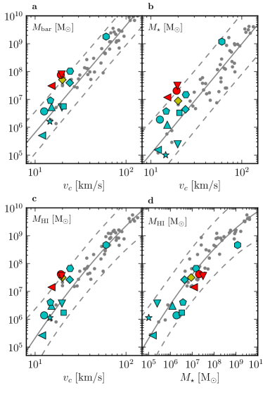
Figure 3.— The baryonic Tully-Fisher relations (a, b, and c) and stellar mass versus H i mass (d). Our simulations compared with the observations (McGaugh, 2012; Bernstein-Cooper et al., 2014). The different symbols represent different simulations, as indicated in Table 1. Blue, red and yellows symbols are simulations with pop iii feedback, without pop iii feedback and the convergence test respectively, while gray circles are observations. The solid lines are the regression lines through the data (linear in a and b, quadratic in c and d) and the dashed lines delimit the $3\sigma$ prediction interval.

3.1. Baryonic Tully-Fisher relation

The baryonic Tully-Fisher relation (BTFR) relates the total baryonic mass to the circular velocity (McGaugh, 2012). Since the inner mass density profile is strongly influenced by the gravitational coupling between gas and dark matter (Cloet-Osselaer et al., 2012), a galaxy’s maximum circular velocity depends non-trivially on the total mass, including dark matter, and its star-formation history. The simulations including pop iii feedback yield dwarf galaxies that lie on the observed BTFR, in terms of total baryonic matter (Fig. 3a) as well as the separate stellar and neutral gas component (Fig. 3b and 3c, respectively). We confirm that these simulations reproduce the observed relation between stellar mass and neutral gas mass as well (Fig. 3d). The control simulations without pop iii feedback fall outside the $3\sigma$ prediction interval of the regression lines fitted to the $v_{c}-M_{\rm bar}$ and $v_{c}-M_{\star}$ observations: they produce $\sim 10$ times too many stars for their circular velocity. In short, our simulations including pop iii feedback succeed in creating faint, gas-dominated dwarf galaxies lying on the BTFR, such as Leo T, Leo P, and Pisces A, while the control simulations without pop iii feedback do not.

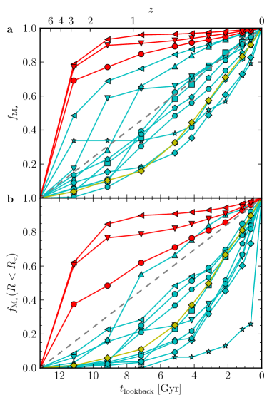
Figure 4.— Cumulative star formation histories. The fraction of the stars formed by a certain lookback time is shown, derived from all stars (a) within the simulation, and (b) within $1~{}R_{e}$. Symbols and colors are the same as in Fig. 3. The dotted lines shows the case for a constant star-formation rate.

3.2. Cumulative star formation histories

In Fig. 4, we present the CSFHs. The upper panel (Fig. 4a) shows the CSFH of all the stars ever formed in the simulation. However, when we only consider the stars currently within a smaller projected distance from the galaxy center, the stellar mass assembly appears significantly more delayed. In Fig. 4b, we present the CSFH of the stars currently within $1~{}R_{e}$, which is more in line with the area covered by current stellar-populations surveys (Weisz et al., 2014). These more central CSFHs look strikingly like those of observed star-forming dwarf galaxies with comparable stellar masses in and near the Local Group (Weisz et al., 2014). In contrast, previous simulations and semi-analytical models generally form too many stars early on (Weinmann et al., 2012).

The cause for the radial dependence of the CSFH is that later stellar generations tend to be born within a more centrally concentrated volume than the earliest stars and that stars can migrate radially and become unbound and dispersed by the tidal forces accompanying merger events. Thus, older stars, which are subjected to more merger events than younger ones, are preferentially affected. In the turbulent ISM of the simulations with pop iii feedback, the first stars show significant outwards radial migration and are subsequently strongly affected by tidal forces. This is much less the case in the control simulations without pop iii feedback. As a consequence, these have much less radially varying CSFHs.

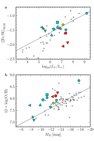
Figure 5.— Metallicities. (a) The stellar Iron abundance and (b) the Oxygen abundance of the ionized gas around star forming regions of the simulations compared with observations of dwarf irregulars (Croxall et al., 2009; Berg et al., 2012; Skillman et al., 2013; Kirby et al., 2013). Symbols and colors are the same as in Fig. 3. The fit to the data in (a) is $\langle\mathrm{[Fe/H]}\rangle_{\mathrm{RGB}}=-2.84+0.21\log_{10}(L_{V}/\,\mathrm{L_{\odot}})$ (Kirby et al., 2013) and in (b) $12+\log(\mathrm{O/H)}=6.27-0.11M_{B}/\,\mathrm{mag}$ (Berg et al., 2012).

3.3. Metallicities

Metallicity measurements for nearby dwarf galaxies are often based on spectroscopic observations of bright stars on the Red Giant Branch (RGB) (e.g. Starkenburg et al., 2010). The number of pop ii RGB stars within the half-light radius of the simulated dwarfs ranges from $\sim 65$ for the faintest one up to $\sim 2000$ for the brightest ones. The estimated number of pop iii RGB stars is zero in all simulated dwarfs presented here. The mean stellar iron abundance of stars that are now on the RGB in the simulated dwarfs agrees very well with the observations (Fig. 5a). The oxygen abundance of the ionized gas surrounding star-forming regions is somewhat on the high side but also in broad agreement with the observations (Fig. 5b). Oxygen is an element forged mostly by core-collapse supernovae while iron is formed abundantly in SNia. The simulations without pop iii feedback form most of their stars early on and therefore have an inordinately large low-metallicity RGB population and hence fall significantly below the observed luminosity-metallicity relation of star-forming dwarf galaxies.

3.4. Metallicity distribution functions

In the previous section, we discussed the global metallicity of the simulated galaxies. However, metallicity distribution functions (MDFs) are available in the literature for many dwarf galaxies (e.g. Kirby et al., 2013). To construct MDFs from our simulations, we again limit ourselves to the stars inside $1~{}R_{e}$ and take the predicted number of RGB stars within each stellar population into account. Fig. 6 shows the MDF of Leo I, taken from Kirby et al. (2013), along with the MDFs of DG15e9b and DG12e9-NP3, which both have stellar masses similar to Leo I. The MDFs of DG12e9-NP3 and the other simulations without pop iii  feedback all have a very long low-metallicity tail: $\sim 1\%$ of the RGB stars is in the form of stars with $\mathrm{[Fe/H]}<-5$. This long tail is absent in observations and such metal-poor stars would be more easily detected. On the other hand, the low-metallicity tail is not present in DG15e9b and the other simulations including pop iii  feedback and the MDF of DG15e9b shows very good agreement with that of Leo I. The simulation has slightly more metal-rich stars which could be because it is still actively star-forming, while Leo I has recently been quenched (Weisz et al., 2014).

This gives further evidence that the first generation of stars did indeed have very different properties than the stars we see today: if such extremely metal-poor stars would have an IMF similar to pop ii  stars, they should be detectable. However to date, no such stars have been found in dwarfs (Starkenburg et al., 2010).

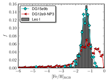
Figure 6.— Metallicity distribution function. The MDFs of a simulation without pop iii  feedback and of one including it, compared to the MDF of Leo I.

3.5. $M_{\star}-M_{\mathrm{halo}}$-relation

The $M_{\star}-M_{\mathrm{halo}}$-relation relates the stellar mass to the dark matter mass and is typically obtained using the abundance matching technique; it is observationally less tractable but theoretically more straightforwardly calculated. We find that the models with pop iii feedback lie within the range predicted by abundance matching techniques (Guo et al., 2010; Moster et al., 2013; Behroozi et al., 2013, respectively the dotted, solid and dashed line in Fig. 7). Note that the simulations with the largest circular velocity do not necessarily have the most massive dark matter halos since the former also depends on the spatial distribution of the matter. At a given halo mass, the scatter on the stellar mass is considerable. This suggests that the abundance matching approach likely looses its applicability in this mass regime. The control simulations without pop iii feedback lie significantly above the predicted $M_{\star}-M_{\mathrm{halo}}$-relations.

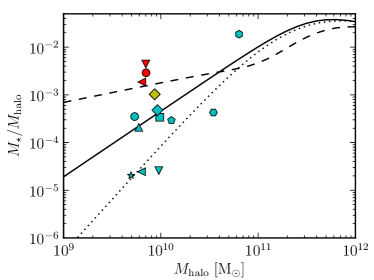
Figure 7.— $M_{\star}-M_{\mathrm{halo}}$-relation. The simulations compared to the abundance matching relations of Guo et al. (2010) (dotted line), Moster et al. (2013) (solid line) and Behroozi et al. (2013) (dashed line). Symbols and colors are the same as in Fig. 3.

3.6. H i  distribution

Fig. 8 shows the H i  distribution, rendered with the publicly available ray tracing package Splotch, overplotted with their H i  density contours, with beam sizes of $40\,\mathrm{pc}$. While this shows that our simulations look qualitatively like real dwarf galaxies, we can look at them more quantitatively.

The substructure in the ISM can be quantified using Fourier transform power spectra of the H i maps. These can be compared with radio observations of dwarf galaxies via the spectral index $\beta$ of the power spectrum $P(k)\propto k^{\beta}$, where $k$ is the wave number (Fig. 9). Like for most real dwarfs in this luminosity regime, this index scatters around $\beta=-11/3\approx-3.67$, the value expected in the case of a three-dimensional Kolmogorov-type incompressible, subsonic turbulence (Zhang et al., 2012). This constitutes a test of the feedback prescription, responsible for blowing “holes” in the neutral gas and keeping the ISM thick and turbulent.

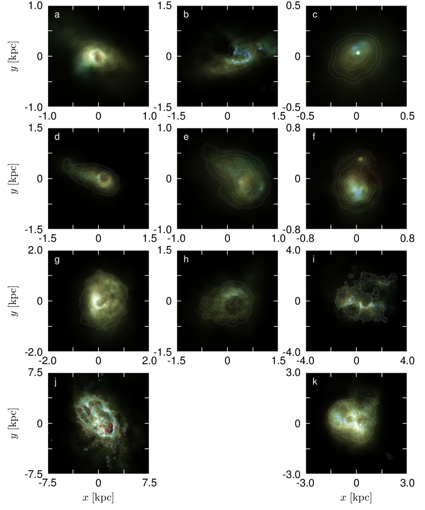
Figure 8.— H i  distribution of the simulations. The gas is rendered using the publicly available ray tracing software Splotch, overplotted with the H i  density isophotes, with the lowest level $N_{\mathrm{HI}}=10^{19}\,\mathrm{cm^{−2}}$ with each next level an increment of a factor 4. The beam size for the H i  contours is $40\,\mathrm{pc}$. (a) DG9e9, (b) DG10e9, (c) DG12e9, (d) DG13e9L, (e) DG13e9E, (f) DG15e9L, (g) DG15e9E, (h) DG20e9, (i) DG50e9, (j) DG1e11 and (k) DG15e9b-CT.

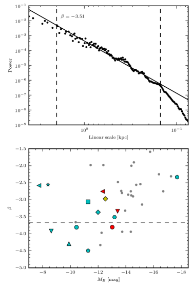
Figure 9.— Spatial power spectra of the H i. (a) The power spectrum of the spatial distribution of HI in DG50e9. The solid grey line shows the power-law fit while the vertical dashed lines show the fitting range. (b) Spectral indices of the power spectra of our simulations, compared with dwarfs in the Little Things survey(Zhang et al., 2012). The horizontal dashed line shows the value of 3D Kolmogorov-type turbulence. Symbols and colors are the same as in Fig. 3.

3.7. Other properties

We also compare the optical colours, half-light radius, the central surface brightness, the central stellar velocity dispersion, the star-formation rate, the Kennicutt-Schmidt relation and the total mass within $300\ \,\mathrm{pc}$ and $1\ R_{e}$ of our models with the observations (Fig. 10a$-$i) . We generally find good agreement between the observed scaling relations and our simulations with pop iii feedback. The control simulations without pop iii feedback are generally more extended and have lower central stellar and mass densities than observed dwarfs.

We note that we reproduce both $M_{0.3}$, the observed total mass within $300\ \,\mathrm{pc}$ (Strigari et al., 2008, Fig. 10h), and $M_{\mathrm{half}}$, the total mass within the half-light radius (Collins et al., 2014, Fig. 10i). Furthermore, although these relations where determined for dSphs, with $L_{V}\lesssim 10^{7}\,\mathrm{L_{\odot}}$, our simulations agree with them over the entire luminosity range, and they predict an extension of this relation to $L_{V}\lesssim 10^{9}\,\mathrm{L_{\odot}}$. For some simulations, $M_{0.3}$ seems to be on the high side however. This is further discussed in the next section.

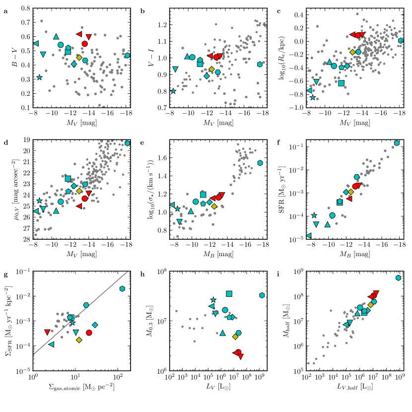
Figure 10.— Other scaling relations. (a) $B-V$ colour, (b) $V-I$ colour, (c) Half light radius $R_{e}$, (d) Central surface brightness in the V-band $\mu_{0,V}$, (e) Stellar velocity dispersion $\sigma_{\star}$, (f) Star formation rate, (g) Kennicutt-Schmidt relation, (h) Total mass within $300\,\mathrm{pc}$, (i) Total mass within $1\ R_{e}$ compared to observations (in grey; Graham & Guzmán, 2003; Hunter & Elmegreen, 2006; Strigari et al., 2008; Vennik & Hopp, 2008; De Rijcke et al., 2009; Makarova et al., 2009; McConnachie, 2012; Rhode et al., 2013; McQuinn et al., 2013; Karachentsev & Kaisina, 2013; Collins et al., 2014; Hopp & Vennik, 2014; Tollerud et al., 2015; Roychowdhury et al., 2015). Symbols and colors are the same as in Fig. 3.

3.8. Cusp versus core

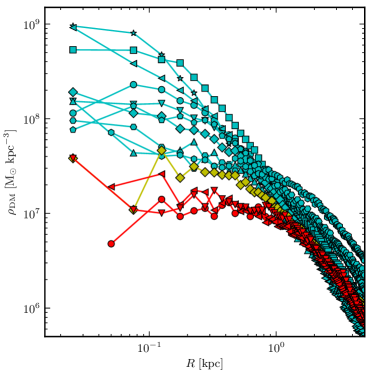
Figure 11.— Dark matter density profiles of the simulations. Symbols and colours are as in Figure 3.

Cosmological simulations including only gravity predict a universal density profile with a cusp in the central regions (Navarro et al., 1996). On the other hand, observations generally favor a cored density profile (de Blok et al., 2008; Salucci et al., 2012). It has been shown that including baryonic effects in simulations can drastically affect the dark matter density profiles and lead to cored density profiles (Read & Gilmore, 2005; Governato et al., 2010; Cloet-Osselaer et al., 2012).

Fig. 11 shows the dark matter density profiles of the simulations. The models can be divided into three groups: DG9e9, DG12e9 and DG15e9a (group 1) have a high dark matter density in the central regions ($\rho_{\mathrm{DM,0}}\sim 10^{9}\,\mathrm{M_{\odot}\ kpc^{-3}}$); group 2 consists of the models without pop iii feedback (DG10e9-NP3, DG12e9-NP3 and DG13e9b-NP3, in red), which have a very low central dark matter density ($\rho_{\mathrm{DM,0}}\sim 10^{7}\,\mathrm{M_{\odot}\ kpc^{-3}}$); the central densities for the remaining models (group 3) lies in between these groups ($\rho_{\mathrm{DM,0}}\sim 10^{8}\,\mathrm{M_{\odot}\ kpc^{-3}}$). We can now have a look to see if these groups manifest themselves in different scaling relations as well. From panels a and c in Fig. 3, one might argue that group 1 lies lower on the BTFR, in terms of $M_{\mathrm{bar}}$ and $M_{\mathrm{HI}}$, although only marginally. However, this is not true in terms of $M_{\star}$ (panel b). Group 3 lies significantly above the BTFR, indicating that they have unrealistic shallow inner density profiles.

Group 3 also has very early SFHs, although this will more likely be the cause of the shallow density profiles, rather than the other way around. Group 1 and group 2 can not be distinguished from their SFHs.

Group 1 lies higher in the stellar metallicity plot (Fig. 5a). One possible explanation is that because of their higher central densities, they can retain their metals more effectively. However, this is not necessarily the only explanation, since the division in groups based on their density profiles was done at $z=0$ and it is not clear how much these density profiles change over time.

There is no clear distinction between group 1 and 2 in the $M_{\star}-M_{\mathrm{halo}}$-relation (Fig 7), indictating that the inner dark matter density profile and the total halo mass influence galaxy properties in different ways.

Not suprisingly, group 1 clearly has smaller $R_{e}$ and $\mu_{0,V}$ (Fig. 10c-d), while group 3 has larger $R_{e}$ and $\mu_{0,V}$. Group 1 and group 3 also have larger, respectively smaller, $M_{0.3}$ (Fig. 10h). DG1e11, which was categorized in group 2, also has a small $R_{e}$ and large $M_{0.3}$, but this is mostly because of its high concentration of stars in its central region, rather than its dark matter properties. Group 1 seems to have a higher stellar velocity dispersion $\sigma_{\star}$, although only very slightly, since $\sigma_{\star}$ was determined at $1\ R_{e}$, so at smaller radii for group 1. Because of the interplay between $R_{e}$ and central density, all groups behave in the same way in terms of $M_{\mathrm{half}}$ (Fig. 10i).

All of this indicates that to identify galaxies with a cusped dark matter density profile, the most likely candidates are the ones with small half-light radii and high total masses within a small, fixed radius. Furthermore, from our simulations it seems unlikely that any dSph galaxies analyzed in Strigari et al. (2008) have a cusped density profile.

3.9. pop iii  to pop ii  transition

The transition of pop iii  to pop ii  star formation occurs, in terms of metallicity, at $\mathrm{[Fe/H]}=-5$ in our models. However, it is not immediately clear at what time this transition occurs and how abrupt it is. Fig. 12 shows the star formation rate of pop iii  stars and of pop ii  stars (in red and blue, respectively) for one of our least massive massive (DG10e9, top panel) and our most massive model (DG1e11, bottom panel). The reason we show DG10e9 rather than DG9e9, is because there is no star formation in this model for $3\lesssim z\lesssim 1$, as seen in Fig. 4. Before 1 Gyr, the pop iii  stars dominated the overall star formation, although there is already some low level pop ii  star formation this early on. This pop iii  star formation declines in time, after which the pop ii  star formation starts dominating the global star formation and after some time, all stars are being formed out of sufficiently enriched gas. The exact time of the last pop iii  stars being formed seems to differ significantly between the two models shown in Fig. 12: the transition occurs much earlier for the least massive model, at $t\approx 1.6\,\mathrm{Gyr}$, while the most massive model still has pop iii  star formation until $t\approx 3.5\,\mathrm{Gyr}$. This trend for later transition times for more massive galaxies is true for all our simulations.

Although this gives a general idea of how and when this transition between star formation modes might have occurred in the universe, we do not wish to overinterpret these results, since the cut-off metallicity is not well constrained and the transition will most likely have been more smoothly than the sharp bimodal model we obtained in our models. However, it does serve as an important check and we confirm that we do not have any pop iii  star formation at low redshift, which would be more easily detected observationally.

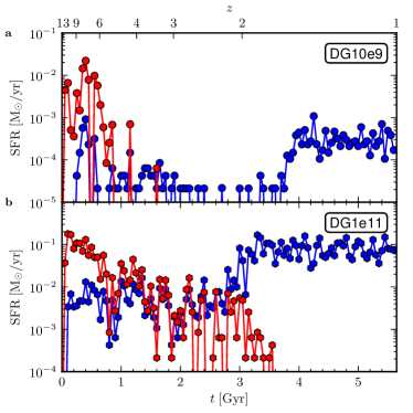
Figure 12.— Transition of pop iii  to pop ii  star formation. Star formation rate of the pop iii  stellar populations (red) and of the pop ii  populations (blue) of DG10e9 (a) and DG1e11 (b), one of our least and our most massive models, respectively. All stellar particles formed in the simulations are taken into account.

4. SUMMARY

We have shown that, with the inclusion of the fierce UV radiation emitted by pop iii stars in numerical simulations, we can reproduce the most important observed properties of isolated gas-rich dwarf galaxies within the $\Lambda$CDM paradigm. This energetic feedback from the very first generation of stars is crucial in suppressing the star-formation rate in a dwarf’s progenitors and thus delaying its star-formation history. We stress that no parameters were fine-tuned to obtain these results.

Furthermore, the expected number of pop iii RGB stars is essentially zero, in agreement with the most metal-poor stars found in dwarf galaxies (Starkenburg et al., 2010).

Of course, there is still room for improvement. For instance, the Oxygen abundances predicted by our simulations are generally on the high side, as is the scatter between the values for the total mass within $300\,\mathrm{pc}$. It remains to be seen if and how these remaining disagreements between models and data can be resolved.

In short, we have provided numerical evidence that the first stars that formed in the early Universe are essential for producing isolated, gas-dominated dwarf galaxies in simulations with broadly the same chemical, kinematical, and structural properties as real dwarf systems in the nearby Universe.

Finally, we wish to stress the crucial importance of mimicking the observations as closely as possible (e.g. by deriving RGB-weighted mean metallicities). This is the only meaningful way in which the validity of numerical simulations can be tested.

References

- Adams et al. (2013) Adams, E. A. K., Giovanelli, R., & Haynes, M. P. 2013, Astrophys. J., 768, 77
- Adams et al. (2015) Adams, E. A. K., Faerman, Y., Janesh, W. F., et al. 2015, Astron. & Astrophys., 573, L3
- Asplund et al. (2009) Asplund, M., Grevesse, N., Sauval, A. J., & Scott, P. 2009, ARA&A, 47, 481
- Behroozi et al. (2013) Behroozi, P. S., Wechsler, R. H., & Conroy, C. 2013, Astrophys. J., 770, 57
- Bell & de Jong (2001) Bell, E. F., & de Jong, R. S. 2001, Astrophys. J., 550, 212
- Benítez-Llambay et al. (2015) Benítez-Llambay, A., Navarro, J. F., Abadi, M. G., et al. 2015, Mon. Not. R. Astron. Soc., 450, 4207
- Benson (2005) Benson, A. J. 2005, Mon. Not. R. Astron. Soc., 358, 551
- Berg et al. (2012) Berg, D. A., Skillman, E. D., Marble, A. R., et al. 2012, Astrophys. J., 754, 98
- Bernstein-Cooper et al. (2014) Bernstein-Cooper, E. Z., Cannon, J. M., Elson, E. C., et al. 2014, Astron. J., 148, 35
- Bertelli et al. (2008) Bertelli, G., Girardi, L., Marigo, P., & Nasi, E. 2008, Astron. & Astrophys., 484, 815
- Bertelli et al. (2009) Bertelli, G., Nasi, E., Girardi, L., & Marigo, P. 2009, Astron. & Astrophys., 508, 355
- Bond et al. (1991) Bond, J. R., Cole, S., Efstathiou, G., & Kaiser, N. 1991, Astrophys. J., 379, 440
- Cen et al. (2004) Cen, R., Dong, F., Bode, P., & Ostriker, J. P. 2004, ArXiv Astrophysics e-prints, astro-ph/0403352
- Chabrier (2003) Chabrier, G. 2003, Astrophys. J. Let., 586, L133
- Clementini et al. (2012) Clementini, G., Cignoni, M., Contreras Ramos, R., et al. 2012, Astrophys. J., 756, 108
- Cloet-Osselaer et al. (2012) Cloet-Osselaer, A., De Rijcke, S., Schroyen, J., & Dury, V. 2012, Mon. Not. R. Astron. Soc., 423, 735
- Cloet-Osselaer et al. (2014) Cloet-Osselaer, A., De Rijcke, S., Vandenbroucke, B., et al. 2014, Mon. Not. R. Astron. Soc., 442, 2909
- Collins et al. (2014) Collins, M. L. M., Chapman, S. C., Rich, R. M., et al. 2014, Astrophys. J., 783, 7
- Croxall et al. (2009) Croxall, K. V., van Zee, L., Lee, H., et al. 2009, Astrophys. J., 705, 723
- de Blok et al. (2008) de Blok, W. J. G., Walter, F., Brinks, E., et al. 2008, Astron. J., 136, 2648
- De Rijcke et al. (2009) De Rijcke, S., Penny, S. J., Conselice, C. J., Valcke, S., & Held, E. V. 2009, Mon. Not. R. Astron. Soc., 393, 798
- De Rijcke et al. (2013) De Rijcke, S., Schroyen, J., Vandenbroucke, B., et al. 2013, Mon. Not. R. Astron. Soc., 433, 3005
- Dutton & Macciò (2014) Dutton, A. A., & Macciò, A. V. 2014, Mon. Not. R. Astron. Soc., 441, 3359
- Efstathiou (1992) Efstathiou, G. 1992, Mon. Not. R. Astron. Soc., 256, 43P
- Faerman et al. (2013) Faerman, Y., Sternberg, A., & McKee, C. F. 2013, Astrophys. J., 777, 119
- Faucher-Giguère et al. (2009) Faucher-Giguère, C.-A., Lidz, A., Zaldarriaga, M., & Hernquist, L. 2009, Astrophys. J., 703, 1416
- Giovanelli et al. (2013) Giovanelli, R., Haynes, M. P., Adams, E. A. K., et al. 2013, Astron. J., 146, 15
- Governato et al. (2010) Governato, F., Brook, C., Mayer, L., et al. 2010, Nature, 463, 203
- Graham & Guzmán (2003) Graham, A. W., & Guzmán, R. 2003, Astron. J., 125, 2936
- Guo et al. (2010) Guo, Q., White, S., Li, C., & Boylan-Kolchin, M. 2010, Mon. Not. R. Astron. Soc., 404, 1111
- Haardt & Madau (1996) Haardt, F., & Madau, P. 1996, Astrophys. J., 461, 20
- Heger & Woosley (2010) Heger, A., & Woosley, S. E. 2010, Astrophys. J., 724, 341
- Hinshaw et al. (2013) Hinshaw, G., Larson, D., Komatsu, E., et al. 2013, Astrophys. J. Suppl., 208, 19
- Hopkins (2015) Hopkins, P. F. 2015, Mon. Not. R. Astron. Soc., 450, 53
- Hopkins et al. (2014) Hopkins, P. F., Kereš, D., Oñorbe, J., et al. 2014, Mon. Not. R. Astron. Soc., 445, 581
- Hopp & Vennik (2014) Hopp, U., & Vennik, J. 2014, Astronomische Nachrichten, 335, 992
- Hunter & Elmegreen (2006) Hunter, D. A., & Elmegreen, B. G. 2006, Astrophys. J. Suppl., 162, 49
- Irwin et al. (2007) Irwin, M. J., Belokurov, V., Evans, N. W., et al. 2007, Astrophys. J. Let., 656, L13
- Janesh et al. (2015) Janesh, W., Rhode, K. L., Salzer, J. J., et al. 2015, Astrophys. J., 811, 35
- Karachentsev & Kaisina (2013) Karachentsev, I. D., & Kaisina, E. I. 2013, Astron. J., 146, 46
- Kirby et al. (2013) Kirby, E. N., Cohen, J. G., Guhathakurta, P., et al. 2013, Astrophys. J., 779, 102
- Klypin et al. (2014) Klypin, A., Yepes, G., Gottlober, S., Prada, F., & Hess, S. 2014, ArXiv e-prints, arXiv:1411.4001
- Makarova et al. (2009) Makarova, L., Karachentsev, I., Rizzi, L., Tully, R. B., & Korotkova, G. 2009, Mon. Not. R. Astron. Soc., 397, 1672
- Marigo et al. (2001) Marigo, P., Girardi, L., Chiosi, C., & Wood, P. R. 2001, Astron. & Astrophys., 371, 152
- McConnachie (2012) McConnachie, A. W. 2012, Astron. J., 144, 4
- McGaugh (2012) McGaugh, S. S. 2012, Astron. J., 143, 40
- McQuinn et al. (2013) McQuinn, K. B. W., Skillman, E. D., Berg, D., et al. 2013, Astron. J., 146, 145
- McQuinn et al. (2015) McQuinn, K. B. W., Cannon, J. M., Dolphin, A. E., et al. 2015, Astrophys. J., 802, 66
- Moster et al. (2013) Moster, B. P., Naab, T., & White, S. D. M. 2013, Mon. Not. R. Astron. Soc., 428, 3121
- Munshi et al. (2013) Munshi, F., Governato, F., Brooks, A. M., et al. 2013, Astrophys. J., 766, 56
- Navarro et al. (1996) Navarro, J. F., Eke, V. R., & Frenk, C. S. 1996, Mon. Not. R. Astron. Soc., 283, L72
- Nomoto et al. (2013) Nomoto, K., Kobayashi, C., & Tominaga, N. 2013, ARA&A, 51, 457
- Oñorbe et al. (2015) Oñorbe, J., Boylan-Kolchin, M., Bullock, J. S., et al. 2015, Mon. Not. R. Astron. Soc., 454, 2092
- Parkinson et al. (2008) Parkinson, H., Cole, S., & Helly, J. 2008, Mon. Not. R. Astron. Soc., 383, 557
- Read & Gilmore (2005) Read, J. I., & Gilmore, G. 2005, Mon. Not. R. Astron. Soc., 356, 107
- Revaz et al. (2009) Revaz, Y., Jablonka, P., Sawala, T., et al. 2009, Astron. & Astrophys., 501, 189
- Rhode et al. (2013) Rhode, K. L., Salzer, J. J., Haurberg, N. C., et al. 2013, Astron. J., 145, 149
- Roychowdhury et al. (2015) Roychowdhury, S., Huang, M.-L., Kauffmann, G., Wang, J., & Chengalur, J. N. 2015, Mon. Not. R. Astron. Soc., 449, 3700
- Ryan-Weber et al. (2008) Ryan-Weber, E. V., Begum, A., Oosterloo, T., et al. 2008, Mon. Not. R. Astron. Soc., 384, 535
- Salucci et al. (2012) Salucci, P., Wilkinson, M. I., Walker, M. G., et al. 2012, Mon. Not. R. Astron. Soc., 420, 2034
- Sand et al. (2015) Sand, D. J., Crnojević, D., Bennet, P., et al. 2015, Astrophys. J., 806, 95
- Sawala et al. (2014) Sawala, T., Frenk, C. S., Fattahi, A., et al. 2014, ArXiv e-prints, arXiv:1406.6362
- Sawala et al. (2015) —. 2015, Mon. Not. R. Astron. Soc., 448, 2941
- Schroyen et al. (2013) Schroyen, J., De Rijcke, S., Koleva, M., Cloet-Osselaer, A., & Vandenbroucke, B. 2013, Mon. Not. R. Astron. Soc., 434, 888
- Schroyen et al. (2011) Schroyen, J., De Rijcke, S., Valcke, S., Cloet-Osselaer, A., & Dejonghe, H. 2011, Mon. Not. R. Astron. Soc.
- Shen et al. (2014) Shen, S., Madau, P., Conroy, C., Governato, F., & Mayer, L. 2014, Astrophys. J., 792, 99
- Skillman et al. (2013) Skillman, E. D., Salzer, J. J., Berg, D. A., et al. 2013, Astron. J., 146, 3
- Springel (2005) Springel, V. 2005, Mon. Not. R. Astron. Soc., 364, 1105
- Springel (2010) —. 2010, Mon. Not. R. Astron. Soc., 401, 791
- Starkenburg et al. (2010) Starkenburg, E., Hill, V., Tolstoy, E., et al. 2010, Astron. & Astrophys., 513, A34
- Stinson et al. (2013) Stinson, G. S., Brook, C., Macciò, A. V., et al. 2013, Mon. Not. R. Astron. Soc., 428, 129
- Strigari et al. (2008) Strigari, L. E., Bullock, J. S., Kaplinghat, M., et al. 2008, Nature, 454, 1096
- Strolger et al. (2004) Strolger, L.-G., Riess, A. G., Dahlen, T., et al. 2004, Astrophys. J., 613, 200
- Susa et al. (2014) Susa, H., Hasegawa, K., & Tominaga, N. 2014, Astrophys. J., 792, 32
- Tollerud et al. (2015) Tollerud, E. J., Geha, M. C., Grcevich, J., Putman, M. E., & Stern, D. 2015, Astrophys. J. Let., 798, L21
- Trujillo-Gomez et al. (2015) Trujillo-Gomez, S., Klypin, A., Colín, P., et al. 2015, Mon. Not. R. Astron. Soc., 446, 1140
- Trujillo-Gomez et al. (2011) Trujillo-Gomez, S., Klypin, A., Primack, J., & Romanowsky, A. J. 2011, Astrophys. J., 742, 16
- Valcke et al. (2008) Valcke, S., De Rijcke, S., & Dejonghe, H. 2008, Mon. Not. R. Astron. Soc., 389, 1111
- Vandenbroucke et al. (2013) Vandenbroucke, B., De Rijcke, S., Schroyen, J., & Jachowicz, N. 2013, Astrophys. J., 771, 36
- Vennik & Hopp (2008) Vennik, J., & Hopp, U. 2008, Astron. & Astrophys., 481, 79
- Verbeke et al. (2014) Verbeke, R., De Rijcke, S., Koleva, M., et al. 2014, Mon. Not. R. Astron. Soc., 442, 1830
- Wang et al. (2015) Wang, L., Dutton, A. A., Stinson, G. S., et al. 2015, Mon. Not. R. Astron. Soc., 454, 83
- Weinmann et al. (2012) Weinmann, S. M., Pasquali, A., Oppenheimer, B. D., et al. 2012, Mon. Not. R. Astron. Soc., 426, 2797
- Weisz et al. (2014) Weisz, D. R., Dolphin, A. E., Skillman, E. D., et al. 2014, Astrophys. J., 789, 147
- Weisz et al. (2012) Weisz, D. R., Zucker, D. B., Dolphin, A. E., et al. 2012, Astrophys. J., 748, 88
- Zhang et al. (2012) Zhang, H.-X., Hunter, D. A., & Elmegreen, B. G. 2012, Astrophys. J., 754, 29