Induced Gravity I: Real Scalar Field

Abstract

We show that classically scale invariant gravity coupled to a single scalar field can undergo dimensional transmutation and generate an effective Einstein-Hilbert action for gravity, coupled to a massive dilaton. The same theory has an ultraviolet fixed point for coupling constant ratios such that all couplings are asymptotically free. However the catchment basin of this fixed point does not include regions of coupling constant parameter space compatible with locally stable dimensional transmutation. In a companion paper, we will explore whether this more desirable outcome does obtain in more complicated theories with non-Abelian gauge interactions.

1 Introduction

The framework for this paper is classically scale invariant quantum gravity, defined by the Lagrangian

$$S_{ho}=\int d^{4}x\sqrt{g}\left[\frac{C^{2}}{2a}+\frac{R^{2}}{3b}+cG\right],$$ (1)

where $R$ is the Ricci scalar, $C$ is the Weyl tensor and $G$ is the Gauss-Bonnet (GB) term. There are three dimensionless coupling constants, $(a,b,c)$. Just about the simplest imaginable scale invariant theory involving gravity and matter fields consists of the above, coupled to a single scalar field with a $\lambda\phi^{4}$ interaction and non-minimal gravitational coupling $\xi R\phi^{2}$. In a recent paper Einhorn:2014gfa , we argued that even this basic theory can undergo dimensional transmutation (DT) à la Coleman-Weinberg (CW) Coleman:1973jx , leading to effective action extrema with nonzero values of the curvature and of the scalar field. It is important to emphasise that, as in the original CW treatment of massless scalar electrodynamics, we restrict ourselves to DT that can be demonstrated perturbatively, in other words, for values of the relevant dimensionless couplings such that higher-order quantum corrections are small.

In this paper, we revisit the results of Ref. Einhorn:2014gfa , while in a companion paper EJ  we extend our approach to the case when the matter sector includes gauge interactions and matter fields with a more complicated scalar sector. Our goal in this will be to demonstrate that the same DT process can be responsible for generating both the Planck mass (with the associated gravitational interactions) and the breaking of a Grand Unified gauge symmetry. In addition we seek a theory such that all dimensional couplings are asymptotically free (AF), with the region of DT within the basin of attraction of an ultra-violet stable fixed point (UVFP) for ratios of couplings. In the case of the minimal model treated here, this is not the case; although a UVFP does exist, with all the dimensionless couplings AF, the DT region is not within its catchment basin.

Before we proceed to gauge theories, however, we have to reassess our previous calculations, for the following reason. Critical to the demonstration of DT in these theories are the results for the one-loop beta-functions, including those of the gravitational self interaction couplings, as well as the contributions of these couplings to the beta-functions for the matter interactions. These were calculated some time ago Fradkin:1981hx ; Fradkin:1981iu ; Avramidi:1985ki ; Avramidi:2000pia ; Buchbinder:1992rb and were summarized in Ref. Buchbinder:1992rb (BOS) for a range of theories. Calculations of this type were revisited recently by Salvio and Strumia Salvio:2014soa (hereafter, SS), with results differing significantly from the earlier ones for the beta-functions for the interactions involving matter fields. We shall see, however, that using the correct beta-functions does not alter the essential conclusions of Ref. Einhorn:2014gfa .

While we endorse the SS form of the beta-functions in general, we differ from them in one respect that impacts the DT calculation. They rewrite $C^{2}$ as follows

$$C^{2}=G+2W$$ (2)

where $W=R_{\mu\nu}^{2}-\frac{1}{3}R^{2}$, so that Eq. (1) becomes

$$S_{ho} = \phantom{-}\int d^{4}x\sqrt{g}\left[\frac{1}{a}{W}+\frac{R^{2}}{3b}+(c+\frac{1}{2a})G\right]$$ (3)

$$= -\int d^{4}x\sqrt{g}\left[\frac{1}{f_{2}^{2}}(\frac{1}{3}R^{2}-R_{\mu\nu}^{2})+\frac{R^{2}}{6f_{0}^{2}}-(c+\frac{1}{2a})G\right],$$

where $a=f_{2}^{2}$ and $b=-2f_{0}^{2}$, and then ignore the $G$ term throughout, on the grounds that it can be expressed locally as a total derivative. The problem with this strategy, and one specifically relevant to the DT paradigm, is that the theory without the $G$ term is not multiplicatively renormalisable Fradkin:1981iu . In curved space but with gravity not quantised, the beta-function associated with the renormalisation of $G$ is the Euler anomaly coefficient; for a recent discussion of its generalisation to the quantised gravity case considered here, see Ref. Einhorn:2014bka . The beta-function for the coefficient of the GB term enters the equation for DT, to be discussed in Section 3.2 below.

We also differ from SS in that we conclude (as before Einhorn:2014gfa ), that we require both $a>0$ and $b>0$, whereas they claim that there is a tachyonic mode if $b>0$ (corresponding to $f_{0}^{2}$ negative in SS). We will discuss this issue further in section 3.

2 Fixed points and asymptotic freedom

One attractive property of pure renormalizable gravity is that it is asymptotically free (AF) Fradkin:1981hx ; Fradkin:1981iu , and this property can be extended to include a matter sector with an asymptotically free gauge theory or even a non-gauge theory. This can be seen as follows. At one-loop order, a gauge coupling $g^{2}$ and the couplings $a$ and $c$ do not mix with the other couplings. In the general case, their beta-functions are (we suppress throughout a factor $(16\pi^{2})^{-1}$ from all one-loop beta-functions):

$$\beta_{g^{2}} =-b_{g}\,(g^{2})^{2}, \qquad\beta_{a} =-b_{2}\,a^{2}, \qquad\beta_{c} =-b_{1},$$ (4a)

$$b_{g} =2(\frac{11}{3}C_{G}-\frac{2}{3}T_{F}-\frac{1}{6}T_{S}), \qquad b_{2} =\frac{133}{10}+N_{a}, \qquad b_{1} =\frac{196}{45}+N_{c},$$ (4b)

where $N_{a}=\left[N_{0}+3N_{F}+12N_{V}\right]/60$ and $N_{c}=\left[N_{0}+\frac{11}{2}N_{F}+62N_{V}\right]/360$. Here $N_{0}$, $N_{F}$ and $N_{V}$ are the numbers of (real) scalar, (two-component) fermion, and (massless) vector fields respectively. (Note that $N_{F}=2N_{\frac{1}{2}}$, the number of fermions as defined in Ref. Einhorn:2014gfa and earlier works.) $C_{G}$, $T_{F}$ and $T_{S}$ are the usual quadratic Casimirs for the pure gauge theory and fermion and scalar representations, with the coefficients of $T_{F}$ and $T_{S}$ in Eq. (4b) also reflecting our choices of two component fermions and real scalars.

It is worth noting at this point that whereas $g$ is AF for $b_{g}>0$ whether it is positive or negative (the sign of the gauge coupling is not a physical observable), for $a$ to be AF we must have $a>0$; $a<0$ corresponds to an unphysical phase with a Landau pole in the UV. Similarly the coupling $c$ is asymptotically free for $c>0,$ since $b_{1}>0$.

The evolution of $b$ is more complicated, because $b$ mixes with the couplings $a,\xi$; moreover, $\beta_{\xi}$ depends on the matter self-couplings. Therefore the evolution of $b$ must be discussed model-by-model. (Note, however, that all three purely gravitational couplings $(a,b,c)$ have beta-functions independent of the gauge couplings (if any) at one loop.) Clearly the possibility of completely AF theories exists for non-gauge theories and for non-abelian gauge theories, but never for an abelian gauge coupling. Thus, the models of interest cannot have gauged U(1) factors, contrary to much of the landscape of string theories.

In a certain sense, the evolution of the two couplings $a$ and $g^{2}$ control the behavior of the other couplings in the theory. To see this, it is useful to rescale the other couplings by one of these two and to express their beta-functions in terms of these ratios. In theories without AF gauge couplings, one must choose $a,$ as we did in our previous papers. In gauge models, it is more convenient Buchbinder:1992rb to rescale by $g^{2}$ instead, replacing the conventional running parameter $dt=d\ln\mu$ by $du=g^{2}(t)dt.$

3 The Minimal Model

The Minimal Model as described in Ref. Einhorn:2014gfa consists of the action

$$S=S_{ho}+S_{\phi},$$ (5)

where

$$S_{\phi}=\int d^{4}x\sqrt{g}\left[\frac{1}{2}(\nabla\phi)^{2}+\frac{\lambda}{4}\phi^{4}-\frac{\xi\phi^{2}}{2}R\right].$$ (6)

Our analysis proceeded in two stages; determination of the fixed point structure of the RG evolution, and demonstration of the existence of extrema determined by DT.

3.1 The Fixed Points

The relevant beta-functions are $\beta_{a,c}$ from Eq. (4), and $\beta_{b,\lambda,\xi}$ given by

$$\beta_{b}\equiv-a^{2}b_{3}(x,\xi),\quad b_{3}(x,\xi)\equiv\left[\frac{10}{3}-5\,x+\left(\frac{5}{12}+\frac{(6\xi+1)^{2}}{24}\right)x^{2}\right],\\$$ (7)

where $x\equiv b/a,$

$$\beta_{\lambda}=18\lambda^{2}+\frac{1}{2}\xi^{2}(5a^{2}+\frac{1}{4}(6\xi+1)^{2}b^{2})+\lambda(5a-\frac{1}{2}(1+6\xi)^{2}b),$$ (8)

and

$$\beta_{\xi}=(6\xi+1)\lambda+\frac{1}{3}\xi\left(\frac{10a^{2}}{b}-(9\xi^{2}+\frac{15}{2}\xi+1)b\right).$$ (9)

As described in the introduction, the results for $\beta_{\lambda,\xi}$ above correspond to those of SS and differ significantly from those employed by us in Ref. Einhorn:2014gfa , based on the beta-functions in the earlier literature Buchbinder:1992rb . For example, although there is a $b\xi^{3}$ term in Eq. (9), there is no $a\xi^{3}$ term; and it is easy to show by an expansion of the metric about flat space and by consideration of the respective contributions of the $a$ and $b$ terms to the graviton propagator that that no such term can arise. In a similar way it can be shown that there can be no $\lambda a\xi^{2}$ term in $\beta_{\lambda}$. However, such terms appear in the expressions corresponding to Eqs. (8),(9) in BOS, which is one reason we believe them to be incorrect.

To determine the asymptotic behavior of the couplings for the above system of beta-functions, we make a couple of redefinitions. We introduce $x=b/a$, (more convenient than $w=a/b$ employed in Ref. Einhorn:2014gfa , it turns out) and $y=\lambda/a$, and a running parameter $u$ such that $du=a(t)dt$.

We then obtain the reduced set of beta-functions:

$$\frac{dx}{du}\equiv\overline{\beta}_{x} =-\frac{10}{3}\left[1-\frac{1099}{200}x+\frac{1}{8}x^{2}+\frac{1}{80}\left(1+6\xi\right)^{2}x^{2}\right];$$ (10a)

$$\frac{d\xi}{du}\equiv\overline{\beta}_{\xi} =\left(6\xi+1\right)y+\frac{\xi}{6}\left(\frac{20}{x}-x(6\xi+1)(3\xi+2)\right);$$ (10b)

$$\frac{dy}{du}\equiv\overline{\beta}_{y} =18y^{2}+y\left(\frac{1099}{60}-\frac{1}{2}x(1+6\xi)^{2}\right)+\frac{\xi^{2}}{8}(20+(6\xi+1)^{2}x^{2}).$$ (10c)

Now from Eq. (10a) it is easy to show that FPs can only exist for $-4.23\leq\xi\leq 3.89$, and that for values of $\xi$ in this range $\overline{\beta}_{x}=0$ has two solutions for $x$, both with $x>0$, with the smaller and larger values of $x$ being IR and UV attractive respectively.

The fixed points of this system of beta-functions (and their nature) are given in Table 1. Remarkably, one of the fixed points with $y=\xi=0$ is UV stable (it is easy to see that a FP with $y=0$ must have $\xi=0$). Since $a$ is AF, this FP corresponds to AF for all the couplings $(a,b,c,\xi,\lambda)$. With regard to the IR stable FP, note that in approaching it from any starting values of the couplings, one would eventually lose perturbative believability since in the IR the coupling $``a"$ approaches a Landau pole in this limit.

We will explore later the catchment basin of the UVFP; but note that since $x>0$ at the FP, it is clear from Eq. (10a) that no region of parameter space with $x<0$ lies in this basin. (Manifestly, for $x<0$, $\overline{\beta}_{x}<0$ as well, so $x\to-\infty$ starting at any value of $x<0$.) Thus, since we have already concluded that $a>0$, we must have $b>0$ as well at any scale from which the couplings can possibly approach the UVFP at higher energies.

	$x$	$\xi$	$y$	Nature
$\!{\bf 1.}$	${\bf 39.78082}$	${\bf 0}$	${\bf 0}$	UV stable
$2.\$	$0.18282$	$0$	$0$	IR stable
$3.\$	$0.18292$	$0.083150$	$-1.005218$	saddle point
$4.\$	$36.9666$	$0.058999$	$0.787391$	saddle point
$5.\$	$43.7762$	$-0.16404$	$-1.01350$	saddle point
$6.\$	$43.7770$	$-0.16551$	$-0.0037756$	saddle point

Table 1: Fixed Points

3.2 Dimensional Transmutation

In Ref. Einhorn:2014gfa we discussed this theory in a totally symmetric gravitational background:

$$R_{\mu\nu\lambda\rho}=\frac{R}{12}\left(g_{\mu\lambda}g_{\nu\rho}-g_{\mu\rho}g_{\nu\lambda}\right),$$ (11)

when the classical action $S_{cl}$ can be written

$$\frac{S_{cl}}{V_{4}}=\frac{1}{3b}+\frac{c}{6}+\frac{1}{4}\left[\lambda r^{2}-2\xi r\right],$$ (12)

where $V_{4}$ is a dimensionless volume element independent of $R$, (we will rescale $S_{cl}$ to absorb $V_{4}$ henceforth) and $r\equiv\phi^{2}/R$. The action has an extremum for $r=r_{0}=\xi/\lambda,$ which is a local minimum if $\lambda>0,$ where it takes the value

$$S_{os}=\frac{1}{6}\left[\frac{2}{b}+c-\frac{3\xi^{2}}{2\lambda}\right].$$ (13)

We showed how the effect of radiative corrections on the action could be analysed by considering the expansion

$$\Gamma(\lambda_{i},r,\rho/\mu)=S_{cl}(\lambda_{i},r)+B(\lambda_{i},r)\log(\rho/\mu)+\frac{C(\lambda_{i},r)}{2}\log^{2}(\rho/\mu)+\ldots,$$ (14)

where $\rho=\sqrt{R},$ and the collection of dimensionless coupling constants $\{a,b,c,\xi,\lambda\}$ has been denoted by $\lambda_{i}$. The value of the effective action for $\rho=\mu$ is simply the classical action.

In Ref. Einhorn:2014gfa , we showed that the condition for an extremum corresponding to DT in this model (and others of this general form) is (to leading order)

$$B_{1}^{(os)}=\sum_{i}\beta_{\lambda_{i}}\frac{\partial S_{os}}{\partial\lambda_{i}}=0,$$ (15)

where $B_{1}^{(os)}$ is the “on-shell” one loop contribution to $B$, with “on-shell” corresponding to $r=r_{0}$. Such an extremum corresponds to a minimum if $\lambda>0$ and

$$\varpi_{2}=\frac{1}{2}\left[C_{2}-{\left(B^{\prime}_{1}\right)^{2}}/{S_{cl}^{{}^{\prime\prime}}}\right]\Big{|}_{r=r_{0}}>0,$$ (16)

where $C_{2}$ is the on-shell leading (two-loop) contribution to $C$, and

$$B^{\prime}_{1}=\frac{\partial}{\partial r}B_{1}(\lambda_{i},r).$$ (17)

Moreover, we used the RG to show that

$$\varpi_{2}=\frac{1}{2}\left[\left(\beta_{\lambda_{i}}^{(1)}\frac{\partial}{\partial\lambda_{i}}\right)^{\!2}\!S_{cl}-\frac{1}{S_{cl}^{{}^{\prime\prime}}}\left(\!\beta_{\lambda_{i}}^{(1)}\frac{\partial}{\partial\lambda_{i}}S^{\prime}_{cl}(\lambda_{i},r)\!\right)^{\!2}\right]\Big{|}_{r=r_{0}}.$$ (18)

We find

$$\begin{split}B_{1}^{(os)}&=\frac{1}{240x^{2}y^{2}}\big{(}1620x^{4}\xi^{6}+540x^{4}\xi^{5}+45x^{4}\xi^{4}-4320x^{3}\xi^{4}y\\ &-360x^{3}\xi^{3}y+60x^{3}\xi^{2}y+900x^{2}\xi^{4}+2880x^{2}\xi^{2}y^{2}+1800x^{2}\xi^{2}y\\ &-480x^{2}\xi y^{2}-826x^{2}y^{2}-2400x\xi^{2}y-2400xy^{2}+1600y^{2}\big{)}.\end{split}$$ (19)

For $\xi=0$, $B_{1}^{(os)}$ is independent of $y$:

$$B_{1}^{(os)}=-\frac{413x^{2}+1200x-800}{120x^{2}},$$ (20)

and $B_{1}^{(os)}=0$ then has solutions $x=-3.465$, $x=0.5591$.

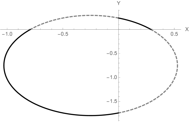
Figure 1: The $B_{1}=0$ ellipse.

We can write $B_{1}^{(os)}$ in terms of $z$, where $z\equiv 3x\xi^{2}/(4y)$:

$$B_{1}^{(os)}=(\frac{20}{3x^{2}}+12\xi^{2})(z-1)^{2}+2(\frac{5}{x}+\xi(2z+1))(z-1)+\frac{1}{3}z(z+1)-\frac{413}{120},$$ (21)

or in terms of $z^{\prime}=z-1$, $\xi^{\prime}=\xi+1/6$:

$$B_{1}^{(os)}=z^{{}^{\prime}2}(12\xi^{{}^{\prime}2}+\frac{20}{3x^{2}})+z^{\prime}(6\xi^{\prime}+\frac{10}{x})-\frac{111}{40}$$ (22)

or

$$B_{1}^{(os)}=12(X+\frac{1}{4})^{2}+\frac{20}{3}(Y+\frac{3}{4})^{2}-\frac{291}{40},$$ (23)

where $X=\xi^{{}^{\prime}}z^{\prime}$ and $Y=z^{\prime}/x$. We thereby express $B_{1}^{(os)}$ in terms of two variables only, in terms of which the solutions to $B_{1}^{(os)}=0$ lie on an ellipse, depicted in Fig. 1, enclosing the region

$$-1.0286<X<0.5286,\quad-1.7946<Y<0.2946.$$ (24)

However, in order to obtain the correct sign for the Einstein term consequent to $\left\langle\phi\right\rangle\neq 0$ (and also by examination of the conformal scalar modesEinhorn:2014gfa ), we must require that $\xi>0$ at the DT scale, corresponding to the constraint

$$\frac{X}{xY}>\frac{1}{6}.$$ (25)

Since we have already concluded that $x>0$ for all points in the UVFP catchment basin, $X$ and $Y$ must have the same signs. Thus, depending on the value of $x$, only portions of the first and third quadrants in Fig. 1 correspond to regions where $\xi>0.$ The allowed range is depicted in Fig. 2a.

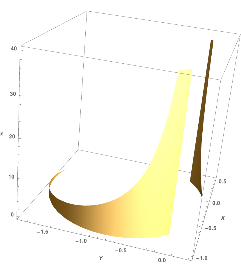
(a) $\xi>0$.

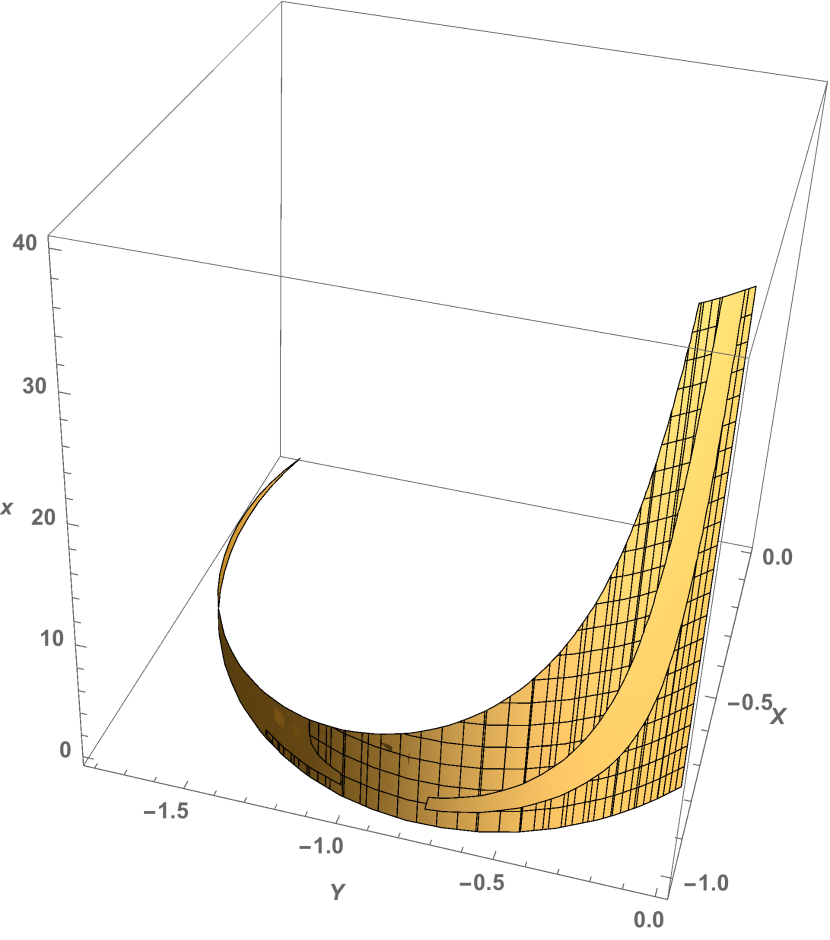
(b) $\xi,\varpi_{2}>0$.

Figure 2: $B_{1}=0$ with constraints.

Similarly, $\varpi_{2}$ may be expressed in terms of $x,\xi$ and $z:$

$$\begin{split}\varpi_{2}&=-a\big{(}10368x^{4}\xi^{4}z^{4}-23328x^{4}\xi^{4}z^{3}+6912x^{4}\xi^{3}z^{4}\\ &+7776x^{4}\xi^{4}z^{2}-6048x^{4}\xi^{3}z^{3}+1728x^{4}\xi^{2}z^{4}+12960x^{4}\xi^{4}z\\ &-9288x^{4}\xi^{3}z^{2}+1152x^{4}\xi^{2}z^{3}+192x^{4}\xi z^{4}-7776x^{4}\xi^{4}+9072x^{4}\xi^{3}z\\ &-3636x^{4}\xi^{2}z^{2}+456x^{4}\xi z^{3}+8x^{4}z^{4}+4320x^{3}\xi^{2}z^{3}+11520x^{2}\xi^{2}z^{4}\\ &-648x^{4}\xi^{3}+648x^{4}\xi^{2}z-222x^{4}\xi z^{2}+34x^{4}z^{3}-8640x^{3}\xi^{2}z^{2}\\ &+1440x^{3}\xi z^{3}-34560x^{2}\xi^{2}z^{3}+3840x^{2}\xi z^{4}+108x^{4}\xi^{2}-84x^{4}\xi z\\ &+15x^{4}z^{2}+4320x^{3}\xi^{2}z-720x^{3}\xi z^{2}+120x^{3}z^{3}+34560x^{2}\xi^{2}z^{2}-6240x^{2}\xi z^{3}\\ &+320x^{2}z^{4}-720x^{3}\xi z+120x^{3}z^{2}-11520x^{2}\xi^{2}z+960x^{2}\xi z^{2}-80x^{2}z^{3}\\ &+330x^{3}z+1440x^{2}\xi z+13388x^{2}z^{2}+19984xz^{3}+3200z^{4}-13628x^{2}z\\ &-39968xz^{2}-9600z^{3}+19984xz+9600z^{2}-3200z\big{)}/(576x^{3}z),\end{split}$$ (26)

or in terms of $(x,X,Y)$:

$$\begin{split}\varpi_{2}&=-a\Big{(}1296X^{4}\big{(}7+4xY\big{)}+108X^{3}\big{(}65+44xY\big{)}\\ &+144X^{2}\big{(}13+(15+11x)Y+(40+15x+x^{2})Y^{2}+40xY^{3}\big{)}\\ &+3X\big{(}57+60(6+x)Y+4(220+90x+3x^{2})Y^{2}+880xY^{3}\big{)}\\ &+Y(1+xY)\big{(}285+7094Y+9992Y^{2}+1600Y^{3}\big{)}\Big{)}/\big{(}288Y(1+xY)\big{)}.\end{split}$$ (27)

Recall that, in order to have local stability (i.e., a positive dilaton mass²,) we must have $\varpi_{2}>0$. Clearly, from Eq. (27), if $X$ and $Y$ are both positive, $\varpi_{2}<0,$ so the first quadrant in Fig. 1 is ruled out. Therefore, since $x>0,\xi>0,$ we must have both $X$ and $Y$ negative. In Fig. 2b, that portion of Fig. 2a having $\varpi_{2}>0$ has been inscribed with a mesh. This is the region of parameter space corresponding to DT that is locally stable with attractive gravity. Note that, unlike $B_{1}$, which has no explicit dependence on $a,$ $\varpi_{2}$ is explicitly proportional to $a$. Further, if we were to restore the suppressed factors of $\kappa\equiv 1/(16\pi^{2})$ in Eqs. (26),(27), $\varpi_{2}$ would be preceded by a factor of $\kappa^{2},$ as is to be expected for a two-loop correction, so that we can expect $\varpi_{2}\ll 1.$

For a consistent model, it must be that the values of the coupling constants in this regime, when run from the DT scale up to higher scales, approach the UVFP. This is a strong constraint and, in fact, fails for this model, as will be discussed in the next section.

4 Basin of Attraction of the UVFP

Although we have determined that the minimal model has a UVFP, we have not delineated the basin of attraction of that point, i.e., the region of all values of the renormalized coupling constants at finite scales whose UV behavior approaches the UVFP. In particular, in order to have a complete theory, the values of the couplings where DT occurs $(B_{1}=0)$ must lie within this catchment basin.

In our earlier paper Einhorn:2014gfa , we showed rather easily that DT occurs in a phase of the theory distinct from the UV catchment basin. With the SS beta-functions, we found a very different value for the UVFP and a different equation for DT. Nevertheless, by means of a hopefully exhaustive exploration of numerical solutions of these equations, we find that, even though there are regions of the $B_{1}=0,$ $\xi>0$ surface that are locally stable $(\varpi_{2}>0)$ it apparently remains true that these regions of DT stability lie outside the UVFP catchment basin. However, we should remark that the DT scale generally lies well outside the neighborhood of the UVFP where a linear approximation suffices, and we have not found a convincing analytical argument in this nonlinear regime.

There is a further limitation to this conclusion associated with the fact that we have neglected fermions and possible Yukawa couplings with our scalar. We shall discuss the inclusion of ”sterile” fermions in the next section, while remarking on the potential impact of Yukawa interactions here. In the absence of gauge and gravitational couplings, Yukawa couplings are never AF. With the addition of renormalizable gravity alone, Yukawa couplings $h_{i}$ are AF for small enough values at the “starting” scale. In fact, they vanish even faster than the gravitational coupling $a.$ However, as we proceed to lower scales, seeking a value where DT occurs, it is not clear that they remain negligible. Our discussion will continue to assume that they can be ignored, but this ought to be explored further since fermions do affect the RG flow of all the couplings and the additional equations involving the Yukawa couplings make the determination of the RG-flows that much more challenging.

Returning to the question of the RG flow, recall that the UVFP is at $(x=x_{0}\approx 39.8,\xi=0,y=0)$. In terms of the variables in Fig. 2, this corresponds to $x\approx 39.8,$ $X\approx-0.167,$ and $Y\approx-0.025.$ The value of $x$ lies in the upper region shown in Fig. 2, with $Y$ near $0$, and $X$ not far from its value at the center of the XY-cylinder ($X=-1/4$). This point lies far from the crosshatched regions shown in Fig. 2b, where locally stable DT occurs. The question is whether, starting near this UVFP and running down to lower scales, the couplings intersect those regions.

First of all, one may not start just anywhere in a neighborhood of the UVFP. We argued in Ref. Einhorn:2014gfa that the EPI converges only if $a,x,\xi,y$ are all positive in the UV. Moreover, we have shown above that at the DT scale, we require $\xi>0$ in order to generate Einstein-Hilbert gravity, and $a,x>0$ in order to lie in the catchment basin of the UVFP. The sign of $a$ cannot change in perturbation theory, and it is positive and monotonically increasing as one runs to lower scales. Since $x_{0}\approx 39.8>0,$ any value of $x$ near there will do. One can see from Eq. (10c) that only the term linear in $y$ is important near the UVFP, and its coefficient is negative, as required for AF. Thus, starting from an initial value $y_{0}>0$, $y$ always increases as $u$ decreases (i.e., as $a$ increases.) Stated otherwise, in flowing to lower scales, $y$ is always repelled from $0.$ That is about all that can be said with certainty. The ratio $x$ can increase or decrease, depending on whether it starts at a point greater or less than $x_{0}$. To first order, $\xi$ may also increase or decrease depending on the sign of $(y-\xi(x_{0}-10/x_{0})/3).$ Thus, even in linear approximation, the behavior is complicated. In the nonlinear regime relevant to DT, the interplay of the different couplings is even harder to discern, and numerical studies bear out that a variety of complicated trajectories can emerge. We have also explored various plots running toward larger $u$ (smaller $a$) starting from points on the $B_{1}^{(os)}=0$ surface, where $\varpi_{2}>0.$ We have found none that lead to the UVFP.

We illustrate two varieties of behaviors of the running couplings in Fig. 3, both starting near the UVFP and running down toward the IR. The starting values for each curve are given in their figure caption. In Fig. 3a, $x,y,\xi$ all decrease toward the IRFP given in the second row of Table 1. In Fig. 3b, $x$ increases above $x_{0},$ and, if we continued following $y,$ we would see that it approaches a singularity at negative $y,$ where perturbation theory breaks down. In both cases, after initially increasing, $y$ peaks and then decreases to negative values of $y$.

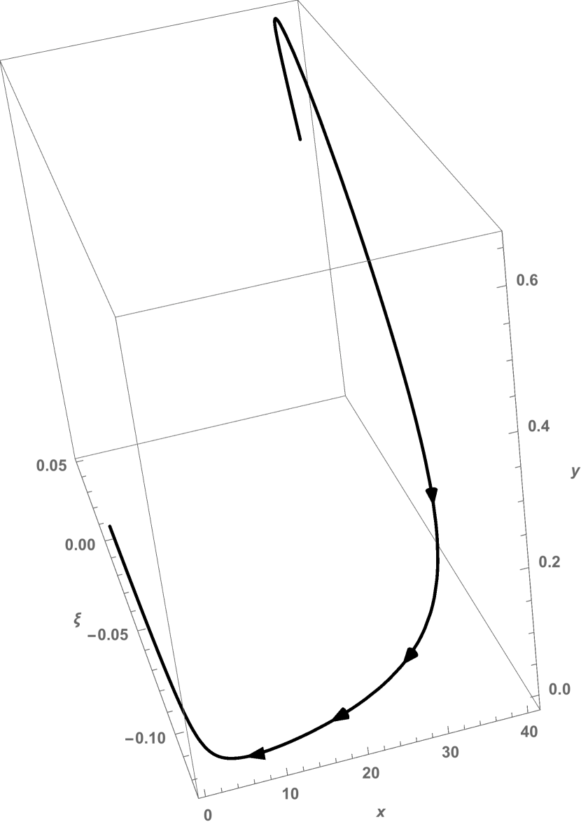
(a) $\!x=38.03,\xi=0.0362,y=0.458$

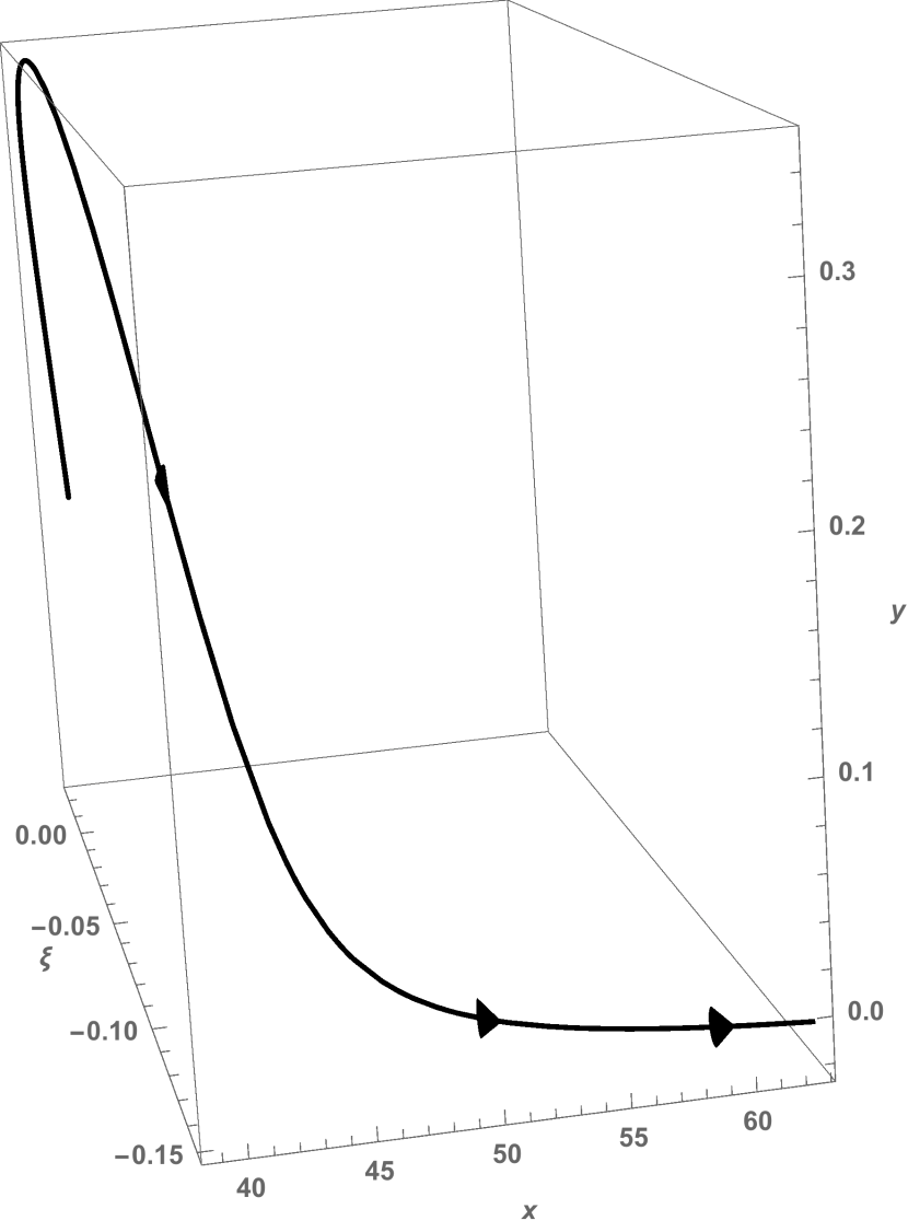
(b) $\!x=39.27,\xi=0.0106,y=0.126$

Figure 3: Running couplings down from near the UVFP.

Our numerical explorations suggest the following conclusions. In order to have $B_{1}^{(os)}=0$ in a range where $\varpi_{2}>0,$ we must have $y\gtrsim 1.3.$ However, starting near the UVFP, it appears that $y$ increases initially but reaches a maximum value at some value of $y\lesssim 0.8.$ That is not hard to believe, since the first and third terms of Eq. (10c) are positive for all values of the couplings and beyond the linear regime, we tend to have $\overline{\beta}_{y}>0.$ Even though $\overline{\beta}_{y}<0$ in the linear regime, it can change sign rather quickly as $u$ decreases. Another way to see the challenge is to rewrite $\overline{\beta}_{y}$ as

$$\overline{\beta}_{y}=18y^{2}+\frac{1099}{60}y+\frac{5}{2}\xi^{2}+x(6\xi+1)^{2}\left(x\frac{\xi^{2}}{8}-\frac{1}{2}y\right).$$ (28)

The only negative term is the last, so one can see the difficulties sustaining $\overline{\beta}_{y}<0$ beyond linear approximation, but exactly how large it can get depends on the starting values of $x$ and $\xi$ and their running. In Fig. 3, we chose examples where the increase of $y$ is relative large, but it turns around long before it approaches $y\approx 1.3.$

We conclude that the catchment basin of the UVFP describes a phase of the theory demarcated from regions where locally stable DT occurs. However, there are regions of parameter space with $a,b,\xi,y$ all positive, where DT occurs at a scale which we may associate with the Planck mass via $M_{P}^{2}\sim\xi\left\langle\phi\right\rangle^{2}$. The effective field theory below this scale is Einstein Gravity with a massive dilaton.

5 Including Fermions

In view of the negative conclusion of the previous section it is worthwhile considering modifying the minimal model by including additional matter fields. The simplest possible such generalisation would involve the inclusion of such fields without additional dimensional couplings. This could clearly be done in a natural way by invoking a global symmetry with respect to which the scalar $\phi$ transformed as a singlet, and adding a fermion multiplet without a quadratic invariant with respect to this symmetry. Under these conditions, there can be no Yukawa couplings, so that the only changes to our calculations would be to alter $b_{1}$ and $b_{2}$ (see Eq. (4b)).

For general $b_{1}$, $b_{2}$ , the reduced beta-function Eq. (10a)-Eq. (10c) become

$$\frac{dx}{du}\equiv\overline{\beta}_{x} =-\frac{10}{3}+(5+b_{2})x-\frac{1}{24}x^{2}\left(10+(1+6\xi)^{2}\right));$$ (29a)

$$\frac{d\xi}{du}\equiv\overline{\beta}_{\xi} =\left(6\xi+1\right)y+\frac{\xi}{6}\left(\frac{20}{x}-x(6\xi+1)(3\xi+2)\right);$$ (29b)

$$\frac{dy}{du}\equiv\overline{\beta}_{y} =18y^{2}+y\left(5+b_{2}-\frac{1}{2}x(1+6\xi)^{2}\right)+\frac{\xi^{2}}{8}(20+(6\xi+1)^{2}x^{2}).$$ (29c)

where with the addition of a fermion multiplet we now have

$$N_{a}=\frac{1}{60}\left(1+3N_{F}\right)\quad\hbox{and}\quad N_{c}=\frac{1}{360}\left(1+\frac{11}{2}N_{F}\right).$$ (30)

Note that Eq. (29b) is unchanged.

It is possible to find the resulting FPs for general $N_{F}$, but the resulting expressions are unwieldy. However, the FP corresponding to the UVFP in Table 1 becomes (for general $b_{1,2}$):

$$x_{FP}=\frac{1}{11}\left(60+12b_{2}+4\sqrt{9b_{2}^{2}+90b_{2}+170}\right),\quad\xi=y=0$$ (31)

or for case of the fermion multiplet:

$$x_{FP}=\frac{1}{55}\left(1099+3N_{F}+\sqrt{1185801+6594N_{F}+9N_{F}^{2}}\right),\quad\xi=y=0.$$ (32)

It is straightforward to show that this FP is UV attractive for arbitrary $N_{F}\geq 0$, or indeed arbitrary $b_{2}>133/10$.

The result for $B_{1}^{(os)}$ (Eq. (23)) becomes

$$B_{1}^{(os)} = 12(X+\frac{1}{4})^{2}+\frac{20}{3}(Y+\frac{3}{4})^{2}-\frac{35}{12}-b_{1}$$ (33)

$$= 12(X+\frac{1}{4})^{2}+\frac{20}{3}(Y+\frac{3}{4})^{2}-\frac{291}{40}-\frac{11}{720}N_{F}.$$

Note that $B_{1}^{(os)}$ depends on $b_{1}$, that is on the beta-function for the coefficient of the Gauss-Bonnet term; so as we remarked in section 2, ignoring this term is not correct, even for $N_{F}=0$. Eq. (23) is replaced by Eq. (33) and we see that ignoring $b_{1}$ would make a significant numerical difference.

However the formulae for $\varpi_{2}$, Eqs. (26),(27), do not change if we keep $b_{1}$ general, but they do depend on $b_{2}$:

$$\varpi_{2} = -\frac{a}{288Y(1+xY)}\Big{(}1296X^{4}\big{(}7+4xY\big{)}+108X^{3}\big{(}65+44xY\big{)}$$ (34)

$$+ 144X^{2}\big{(}13+(15+11x)Y+(40+15x+x^{2})Y^{2}+40xY^{3}\big{)}$$

$$+ 3X\big{(}57+60(6+x)Y+4(220+90x+3x^{2})Y^{2}+880xY^{3}\big{)}$$

$$+ 5Y(1+xY)\big{(}57+4(18b_{2}+115)Y+48(2b_{2}+15\,)Y^{2}+320Y^{3}\big{)}\Big{)}.$$

We see that the property that local stability requires both $X$ and $Y$ negative is sustained by this generalisation.

6 Conclusions

We have shown that the theory consisting of renormalisable $R^{2}$ quantum gravity coupled to a single scalar field in a scale-invariant way undergoes dimensional transmutation in a manner which can be credibly described by perturbation theory. Below the DT scale, the theory describes Einstein gravity coupled to a scalar dilaton which obtains a mass through spontaneous breaking of scale invariance. We also found that the theory possesses an Ultra-Violet Fixed Point for coupling ratios, such that all the couplings tend to zero as this FP is approached, with the ratio $x=b/a\to 39.8$. Since $a>0$ is required for Asymptotic Freedom, it follows that $b>0$ in the neighbourhood of the FP. In fact in Ref. Einhorn:2014gfa  we argued that both $a,b>0$ (and $\lambda>0$) are required for convergence of the EPI, so the theory is well behaved in the UV for couplings in the FP catchment basin. It should be noted that here we appear to differ from SS, who in our notation seem to require $a>0$ but $b<0$.

However, although the region of parameter space for the dimensionless couplings where DT occurs includes a region with $x,y>0$ and also $\xi>0$, which we require to generate Einstein gravity, it turns out that the theory becomes strongly coupled at higher scales, with couplings approaching Landau poles. Thus this particular theory is not an ultraviolet (UV) complete theory of Einstein gravity. This is a disappointing outcome since there are regions of parameter space where all the couplings are asymptotically free, with coupling constant ratios approaching the UV Fixed Point.

Although we have adopted the beta-functions of SS, we wish to emphasize that our results differ from theirs in significant ways. Their determination of the analog of our function $B_{1}$ would omit any contribution from the Gauss-Bonnet term. Moreover, their criteria for determination of the DT scale involves an approximation that differs significantly from ours.

Further, we determined the two-loop value of the dilaton mass² in order to ascertain whether the DT extrema are locally stable. Finally, we explored the basin of attraction of the UVFP, showing via the renormalization group that there are apparently no paths in this catchment that, at lower scales, undergo DT in a manner that satisfies the physical constraints. We therefore regard their applications of these sorts of classically scale-invariant models somewhat skeptically.

In a subsequent paper EJ  we will extend our formalism to Grand Unified Theories, where we show that once again it is possible to construct completely Asymptotically Free models, with coupling constant ratios approaching fixed points. It transpires that to achieve this it is necessary to add enough matter fields to make the one loop gauge beta-function coefficient as numerically small as possible (while, obviously, remaining negative). This was demonstrated long ago in flat space Cheng:1973nv and remains true in the presence of gravitational corrections Buchbinder:1989ma ; Buchbinder:1989jd .

It is also possible to exhibit GUT models which undergo Dimensional Transmutation in the same manner as we have described here. Moreover, by appropriate choice of scalar representation it is possible to arrange that the same scalar vacuum expectation value generated by DT both produces Einstein gravity and breaks the Grand Unified symmetry. The crucial question (which had a disappointing answer in the model of this paper) is whether there are DT regions of parameter space in the catchment basin of a UVFP. We will answer this question in Ref. EJ , where we construct a model based on the gauge group SO(10) with an adjoint scalar representation. This scalar acquires a vev via DT, breaking the SO(10) symmetry so as to leave unbroken the maximal subgroup SU(5)$\otimes$U(1). Moreover, we have shown that there is a region of parameter space where DT occurs that satisfies all our requirements (such as generation of a “right-sign” Einstein term) and is in the catchment of a UV fixed point such that all the couplings are asymptotically free. We thus have the basis for a UV complete extension of the Standard Model.

Of course problems remain to be solved, not least of which being the origin of the electroweak scale. There is also the issue of the (doubtful) unitarity of $R^{2}$ gravity, in both the minimal model considered here and in the gauge theory extensions. We discussed this problem briefly in Ref. Einhorn:2014gfa and will do so again Ref. EJ ; suffice to say for now that we believe it is possible that the combination of AF (at high energies) with DT as we run towards the IR (so that if DT did not occur the theory would become strongly coupled) leads to its solution.

- (1) M. B. Einhorn and D. R. T. Jones, “Naturalness and Dimensional Transmutation in Classically Scale-Invariant Gravity,” JHEP 1503 (2015) 047 [arXiv:1410.8513 [hep-th]].
- (2) S. R. Coleman and E. J. Weinberg, “Radiative Corrections as the Origin of Spontaneous Symmetry Breaking,” Phys. Rev. D 7 (1973) 1888.
- (3) I. L. Buchbinder, “Mechanism For Induction Of Einstein Gravitation,” Sov. Phys. J. 29 (1986) 220.
- (4) G. Cognola and I. L. Shapiro, “Back reaction of vacuum and the renormalization group flow from the conformal fixed point,” Class. Quant. Grav. 15 (1998) 3411 [hep-th/9804119].
- (5) I. L. Shapiro and A. G. Zheksenaev, “Gauge dependence in higher derivative quantum gravity and the conformal anomaly problem,” Phys. Lett. B 324 (1994) 286.
- (6) M. B. Einhorn and D. R. T. Jones, “Induced Gravity II: Grand Unified Theories” (in preparation).
- (7) E. S. Fradkin and A. A. Tseytlin, “Renormalizable Asymptotically Free Quantum Theory of Gravity,” Phys. Lett. B 104 (1981) 377.
- (8) E. S. Fradkin and A. A. Tseytlin, “Renormalizable asymptotically free quantum theory of gravity,” Nucl. Phys. B 201 (1982) 469.
- (9) I. G. Avramidi and A. O. Barvinsky, “Asymptotic Freedom In Higher Derivative Quantum Gravity,” Phys. Lett. B 159 (1985) 269.
- (10) I. G. Avramidi, “Heat kernel and quantum gravity,” Lect. Notes Phys. M 64 (2000) 1.
- (11) I. L. Buchbinder, S. D. Odintsov and I. L. Shapiro, “Effective action in quantum gravity,” Bristol, UK: IOP (1992).
- (12) A. Salvio and A. Strumia, “Agravity,” JHEP 1406 (2014) 080 [arXiv:1403.4226 [hep-ph]].
- (13) M. B. Einhorn and D. R. T. Jones, “Gauss-Bonnet coupling constant in classically scale-invariant gravity,” Phys. Rev. D 91 (2015) 8, 084039 [arXiv:1412.5572 [hep-th]].
- (14) T. P. Cheng, E. Eichten and L. F. Li, “Higgs Phenomena in Asymptotically Free Gauge Theories,” Phys. Rev. D 9 (1974) 2259.
- (15) I. L. Buchbinder, et al., “Asymptotically free grand unification models with quantum R**2 gravitation,” Sov. J. Nucl. Phys. 49, 544 (1989) [Yad. Fiz. 49, 876 (1989)].
- (16) I. L. Buchbinder, et al., “The Stability of Asymptotic Freedom in Grand Unified Models Coupled to Gravity,” Phys. Lett. B 216 (1989) 127.