Selective inference in regression models with groups of variables

Abstract

We discuss a general mathematical framework for selective inference with supervised model selection procedures characterized by quadratic forms in the outcome variable. Forward stepwise with groups of variables is an important special case as it allows models with categorical variables or factors. Models can be chosen by AIC, BIC, or a fixed number of steps. We provide an exact significance test for each group of variables in the selected model based on appropriately truncated $\chi$ or $F$ distributions for the cases of known and unknown $\sigma^{2}$ respectively. An efficient software implementation is available as a package in the R statistical programming language.

and t1Supported in part by NIH grant 5T32GMD96982. t2Supported in part by NSF grant DMS 1208857 and AFOSR grant 113039.

1 Introduction

A common strategy in data analysis is to assume a class of models $\mathcal{M}$ specified a priori contains a particular model $M\in\mathcal{M}$ which is well-suited to the data. Unfortunately, when the data has been used to pick a particular model $\hat{M}$, inference about the selected model is usually invalid. For example, in the regression setting with many predictors if the “best” predictors are chosen by lasso or forward stepwise then the classical $t$, $\chi^{2}$, or $F$ tests for their coefficients will be anti-conservative. The most widespread solution is data splitting, where one subset of the data is used only for model selection and another subset is used only for inference. This results in a loss of accuracy for model selection and power for inference.

Recently, Lockhart et al. (2014); Lee et al. (2015) developed methods of adjusting the classical significance tests to account for model selection. These methods make use of the fact that the model chosen by lasso and forward stepwise can be characterized by affine inequalities in the data. Inference conditional on the selected model requires truncating null distributions to the affine selection region. The present work provides a new and more general mathematical framework based on quadratic inequalities. Forward stepwise with groups of variables serves as the main example which we develop in some detail.

Allowing variables to be grouped provides important modeling flexibility to respect known structure in the predictors. For example, to fit hierarchical interaction models as in Lim and Hastie (2013), non-linear models with groups of spline bases as in Chouldechova and Hastie (2015), or factor models where groups are determined by scientific knowledge such as variables in common biological pathways. Further, in the presence of categorical variables, without grouping a model selection procedure may include only some subset of the levels that variable.

All methods described here are implemented in the selectiveInference R package (Tibshirani et al., 2015) available on CRAN.

1.1 California county health data example

Information on health and various other indicators has been aggregated to the county level by University of Wisconsin Population Health Institute (2015). We attempt to fit a linear model for California counties with outcome given by log-years of potential life lost, and search among 31 predictors using forward stepwise. This example has groups only of size 1, but still serves to illustrate the procedure. With the BIC criteria for choosing model size the resulting model has 8 variables listed in Table 1. The naive $p$-values computed from standard hypothesis tests for linear regression models are biased to be small because we chose the 8 best predictors out of 31.

Table 1: Significance test $p$-values for predictors chosen by forward stepwise with BIC.

Step	Variable	Naive	Selective
1	%80th Percentile Income	$<$0.001	0.001
2	Injury Death Rate	$<$0.001	0.086
3	Chlamydia Rate	0.078	0.287
4	%Obese	$<$0.001	0.170
5	%Receiving HbA1c	$<$0.001	0.335
6	%Some College	0.005	0.864
7	Teen Birth Rate	0.071	0.940
8	Violent Crime Rate	0.067	0.179

The selective $p$-values reported here are the $T\chi$ statistics described in Section 3. These have been adjusted to account for model selection. Using the data to select a model and then conducting inference about that model means we are randomly choosing which hypotheses to test. In this scenario, Fithian, Sun and Taylor (2014) propose controlling the selective type 1 error defined as

$$\mathbb{P}_{M,H_{0}(M)}(\text{reject }H_{0}|M\text{ selected}).$$ (1)

The notation $H_{0}(M)$ emphasizes the fact that the hypothesis depends upon the model $M$. Scientific studies reporting $p$-values which control (1) would not suffer from model selection bias, and consequently would have greater replicability.

One of the most common methods which controls selective type 1 error is data splitting, where independent subsets of the data are used for model selection and inference separately. Unfortunately, by using less data to select the model and less data to conduct tests this method suffers from loss of model selection accuracy and lower power. The $T\chi$ and $T_{F}$ hypothesis tests described in the present work control (1) while using the whole data for both selection and inference.

1.2 Background: the affine framework

Many model selection procedures, including lasso, forward stepwise, least angle regression, marginal screening, and others, can be characterized by affine inequalities. In other words, for each $m\in\mathcal{M}$ there exists a matrix $A_{m}$ and vector $b_{m}$ such that $\hat{M}(y)=m$ is equivalent to $A_{m}y\leq b_{m}$. Hence, assuming

$$y=\mu+\epsilon,\quad\epsilon\sim N(0,\sigma^{2}I)$$ (2)

we can carry out inference conditional on $\hat{M}(y)=m$ by constraining the multivariate normal distribution to the polyhedral region $\{z:A_{m}z\leq b_{m}\}$.

One limitation of these methods is that the definition of a model $m$ includes not only the active set $E$ of variables chosen by the lasso or forward stepwise, but also their signs. Without including signs, the model selection region becomes a union of $2^{|E|}$ polytopes. Details are provided in Lee et al. (2015). The forward stepwise and least angle regression cases without groups of variables appear in Tibshirani et al. (2014).

In an earlier work, Loftus and Taylor (2014) iterated the global null hypothesis test of Taylor, Loftus and Tibshirani (2015) at each step of forward stepwise with groups. The test there is only exact at the first step where it coincides with the $T\chi$ test described here, and empirically it was increasingly conservative at later steps. The present work does not pursue sequential testing, and instead conducts exact tests for all variables included in the final model.

1.3 The quadratic framework

Our approach will exploit the structure of model selection procedures characterized by quadratic inequalities in the following sense.

Definition 1.1.

A quadratic model selection procedure is a map $M:\mathcal{X}\to\mathcal{M}$ determining a model $m=M(y)$, such that for any $m\in\mathcal{M}$

$$E_{m} :=\{y:M(y)=m\}=\bigcap_{j\in J_{m}}E_{m,j},$$ (3)

$$E_{m,j} :=\{y:y^{T}Q_{m,j}y+a_{m,j}^{T}y+b_{m,j}\geq 0\}$$

The power of this definition lies in the ease with which we can compute one-dimensional slices through $E_{m}$. This enables us to compute closed-form results for certain one-dimensional statistics and to potentially implement hit-and-run sampling schemes. Consider tests based on $T^{2}:=\|Py\|^{2}_{2}$ for some fixed projection matrix $P$. Write $u=Py/T$, $z=y-Py$, and substitute $uT+z$ for $y$ in the definition (3). Conditioning on $z$ and $u$, the only remaining variation is in $T$, and the equations above are univariate quadratics. This allows us to determine the truncation region for $T$ induced by the model selection $M(y)=m$. We now apply this approach and work out the details for several examples. The example in Section 4 is a slight extension beyond the quadratic framework that illustrates how this approach may be further generalized.

2 Forward stepwise with groups

This section establishes notation and describes the particular variant of grouped forward stepwise referred to throughout this paper. Readers familiar with the statistical programming language R may know of this algorithm as the one implemented in the step function. Because we are interested in groups of variables, the stepwise algorithm is not stated in terms of univariate correlations the way forward stepwise is often presented.

We observe an outcome $y\sim N(\mu,\sigma^{2}I)$ and wish to model $\mu$ using a sparse linear model $\mu\approx X\beta$ for a matrix of predictors $X$ and sparse coefficient vector $\beta$. We assume the matrix $X$ is subdivided a priori into groups

$$X=\begin{bmatrix}X_{1}&X_{2}&\cdots&X_{G}\end{bmatrix}$$ (4)

with $X_{g}$ denoting the submatrix of $X$ with all columns of the group $g$ for $1\leq g\leq G$. Forward stepwise, described in Algorithm 1, picks at each step the group minimizing a penalized residual sums of squares criterion. The penalty is an AIC criterion penalizing group size, since otherwise the algorithm will be biased toward selecting larger groups. First we describe the case where $\sigma^{2}$ is known. With a parameter $k\geq 0$, the penalized RSS criterion is

$$g_{1}=\operatorname*{arg\,min}\|(I-P^{1}_{g})y\|_{2}^{2}+k\sigma^{2}\text{Tr}(P^{1}_{g})$$ (5)

where $P^{1}_{g}:=X_{g}X_{g}^{\dagger}$ and $\text{Tr}(P^{1}_{g})$ is the degrees of freedom used by $X_{g}$. Minimizing this with respect to $g$ is equivalent to maximizing

$$RSS_{1}(g):=y^{T}P^{1}_{g}y-k\sigma^{2}\text{Tr}(P^{1}_{g})$$ (6)

Note that the event $E_{1}:=\{z:\operatorname*{arg\,max}RSS_{1}(g)=g_{1}\}$ can be decomposed as an intersection

$$E_{1}=\bigcap_{g\neq g_{1}}\{z:z^{T}Q^{1}_{g}z+k^{1}_{g}\geq 0\}$$ (7)

where $Q^{1}_{g}:=P^{1}_{g_{1}}-P^{1}_{g}$ and $k^{1}_{g}:=k\sigma^{2}\text{Tr}(P^{1}_{g_{1}}-P^{1}_{g})$. We ignore ties and use $>$ and $\geq$ interchangeably. Ties do not occur with probability 1 under fairly general conditions on the design matrix.

Data: An $n$ vector $y$ and $n\times p$ matrix $X$ with $G$ groups, complexity penalty parameter $k\geq 0$

Result: Ordered active set $A$ of groups included in the model at each step

begin

       $A\leftarrow\emptyset$, $A^{c}\leftarrow\{1,\ldots,G\}$, $r_{0}\leftarrow y$

       for $s=1$ to $steps$ do

             $P_{g}\leftarrow X_{g}X_{g}^{\dagger}$

             $g^{*}\leftarrow\operatorname*{arg\,max}_{g\in A^{c}}\{r_{s-1}^{T}P_{g}r_{s-1}-k\sigma^{2}\text{Tr}(P_{g})\}$

            

            $A\leftarrow A\cup\{g^{*}\}$, $A^{c}\leftarrow A^{c}\backslash\{g^{*}\}$

             for $h\in A^{c}$ do

                   $X_{h}\leftarrow(I-P_{g^{*}})X_{h}$

                  

            $r_{s}\leftarrow(I-P_{g^{*}})r_{s-1}$

            

      return $A$

Algorithm 1 Forward stepwise with groups, $\sigma^{2}$ known

After adding a group of variables to the active set, we orthogonalize the outcome and the remaining groups with respect to the added group. So, at step $s>1$, we have $A_{s}=\{g_{1},g_{2},\ldots,g_{s-1}\}$ and define

$$P_{s} :=(I-P^{s-1}_{g_{s-1}})(I-P^{s-2}_{g_{s-2}})\cdots(I-P^{1}_{g_{1}})$$ (8)

$$r_{s} :=P_{s}y,\quad X_{g}^{s}:=P_{s}X_{g},\quad P_{g}^{s}:=X_{g}^{s}(X_{g}^{s})^{\dagger}$$

Then the group added at step $s$ is

$$g_{s}=\operatorname*{arg\,max}_{g\in A^{c}}r_{s}^{T}P^{s}_{g}r_{s}-k\sigma^{2}\text{Tr}P^{s}_{g}$$ (9)

Now for

$$E_{s}:=\{z\in E_{s-1}:\operatorname*{arg\,max}RSS_{s}(g)=g_{s}\}$$ (10)

we have

$$E_{s}=E_{s-1}\cap\bigcap_{\begin{subarray}{c}g\in A_{s}^{c}\\ g\neq g_{s}\end{subarray}}\{z:z^{T}P_{s}Q^{s}_{g}P_{s}z+k^{s}_{g}\geq 0\}\\$$ (11)

where $Q^{s}_{g}:=P^{s}_{g_{s}}-P^{s}_{g}$ and $k^{s}_{g}:=\sigma^{2}k\text{Tr}(P^{s}_{g_{s}}-P^{s}_{g})$. We have established the following lemma.

Lemma 2.1.

The selection event $E$ that forward stepwise selects the ordered active set $A_{s}=\{g_{1},g_{2},\ldots,g_{s}\}$ can be written as an intersection of quadratic inequalities all of the form $y^{T}Qy+b\geq 0$, which satisfies Definition 1.1.

We leverage this fact to compute truncation intervals for selective significance tests based on one-dimensional slices through $E$. When $\sigma$ is known, the truncated $\chi$ test statistic $T\chi$ described in Section 3 is used to test the significance of each group in the active set. For unknown $\sigma$, the corresponding truncated $F$ statistic $T_{F}$ is detailed in Section 4. The unknown $\sigma^{2}$ case alters the above algorithm by changing the RSS criteria to the form

$$g_{s}=\operatorname*{arg\,max}(r_{s}^{T}r_{s}-r_{s}^{T}P_{g_{s}}^{s}r_{s})\exp(-k\text{Tr}(P_{g_{s}}^{s}))$$ (12)

This merely replaces the additive constant with a multiplicative one. Finally, we note that $k=2$ corresponds to the classic AIC criterion Akaike (1973), $k=\log(n)$ yields BIC Schwarz et al. (1978), and $k=2\log(p)$ gives the RIC criterion of Foster and George (1994). The extension of Algorithm 1 to allow stopping using the AIC criterion is given later in Section 5.

2.1 Linear model and null hypothesis

Once forward stepwise has terminated yielding an active set $A$, we wish to conduct inference about the model regressing $y$ on $X_{A}$ where the subscript denotes all columns of $X$ corresponding to groups in $A$. Throughout this paper we do not assume the linear model is correctly specified, i.e. it is possible that $\mu\neq X_{A}\beta$ for all $\beta$. This is a strength for robustness purposes, however it also results in lower power against alternatives where the linear model is correctly specified and forward stepwise captures the true active set.

Even when the linear model is not correctly specified, there is still a well-defined best linear approximation

$$\beta_{A}^{*}:=\operatorname*{arg\,min}\mathbb{E}[\|y-X_{A}\beta\|_{2}^{2}]$$ (13)

with the usual estimate given by the least squares fit $\hat{\beta}_{A}=X_{A}^{\dagger}y$.

The probability modeling assumption throughout this paper is (2), and the null hypothesis for a group $g$ in $A$ is given by

$$H_{0}(A,g):\beta_{A,g}^{*}=0$$ (14)

where $\beta_{A,g}$ denotes the coordinates of coefficients for group $g$ in the linear model determined by $X_{A}$. Note that this null hypothesis depends on $A$, as the coefficients for the same group $g$ in a different active set $A^{\prime}\neq A$ with $g\in A^{\prime}$ have a different meaning, namely they are regression coefficients controlling for the variables in $A^{\prime}$ rather than in $A$. Several equivalent formulations of (14) are

$$H_{0}(A,g) :X_{g}^{T}(I-P_{A/g})\mu=0,$$ (15)

$$H_{0}(A,g) :P_{g}(I-P_{A/g})\mu=0,$$

$$H_{0}(A,g) :\tilde{P}_{g}\mu=0$$

where $\tilde{P}_{g}$ is the projection onto the column space of $(I-P_{A/g})X_{g}$. We use these forms to emphasize that the probability model for $y$ is determined by $\mu$ and not by $\beta^{*}$.

3 Truncated $\chi$ significance test

We now describe our significance test for a group of variables $g$ in the active set $A$, under the probability model $y\sim N(\mu,\sigma^{2}I)$ where we assume $\sigma$ is known or can be estimated independently from $y$. Section 4 concerns the case where $\sigma$ is unknown.

3.1 Test statistic, null hypothesis, and distribution

First we consider forward stepwise with a fixed, deterministic number of steps $S$. Choosing $S$ with an AIC-type criterion requires some additional work described in Section 5. Let $A$ denote the ordered active set and $E$ the event that $A=\{g_{1},g_{2},\ldots,g_{S}\}$. With $\tilde{X}_{g}=(I-P_{A/g})X_{g}$, let $\tilde{X}_{g}=U_{g}D_{g}V_{g}^{T}$ be the singular value decomposition of $\tilde{X}_{g}$. Note that $\tilde{P}_{g}=U_{g}U_{g}^{T}$. In this notation, without model selection, the test statistic and null distribution

$$T^{2}:=\sigma^{-2}\|U_{g}^{T}y\|_{2}^{2}\sim\chi^{2}_{\text{Tr}(\tilde{P}_{g})}\text{ under }H_{0}(A,g)$$ (16)

form the usual regression model hypothesis test for the group $g$ of variables in model $X_{A}$ when $\sigma^{2}$ is known.

Let $u\propto\tilde{P}_{g}y$ be a unit vector, so $y=z+Tu$ where $z=(I-\tilde{P}_{g})y$. Under the null, $(T,z,u)$ are independent because $\tilde{P}_{g}y$ and $z$ are orthogonal and $(T,u)$ are independent by Basu’s theorem. We condition on $z$ and $u$ without changing the test under the null, but it should be noted that this may result in some loss of power under certain alternatives. Now the only remaining variation is in $T$, and we still have $T^{2}\sim\chi^{2}_{\text{Tr}(\tilde{P}_{g})}$ if there is no model selection. Finally, to obtain the selective hypothesis test we apply the following theorem with $P_{A}=\tilde{P}_{g}$.

Theorem 3.1.

If $y\sim N(\mu,\sigma^{2}I)$ with $\sigma^{2}$ known, and $P_{A}\mu=0$ for some $P_{A}$ which is constant on $\{M(y)=A\}$, then defining $r:=\text{Tr}(P_{A})$, $R:=P_{A}y$, $u:=R/\|R\|_{2}$, $z:=y-R$, the truncation interval $M_{A}:=\{t\geq 0:M(ut\sigma+z)=A\}$, and the observed statistic $T=\|R\|_{2}/\sigma$, we have

$$T|(A,z,u)\sim\left.\chi_{r}\right|_{M_{A}}$$ (17)

where the vertical bar denotes truncation. Hence, with $f_{r}$ the pdf of a central $\chi_{r}$ random variable

$$T\chi:=\frac{\int_{M_{A}\cap[T,\infty]}f_{r}(t)dt}{\int_{M_{A}}f_{r}(t)dt}\sim U[0,1]$$ (18)

is a $p$-value.

Proof.

First consider $P_{A}=P$ as fixed independently of $y$, and write $T_{P},z_{P},u_{P}$, and $M_{A}(P)$ to emphasize these are determined by $P$. Without selection, we know $(T_{P},z_{P},u_{P})$ are independent and $T_{P}|(z_{P},u_{P})\sim\chi_{r}$. Since the selection event is determined entirely by $M(u_{P}t\sigma+z_{P})=A$, conditioning further on $\{M(y)=A\}$ has the effect of truncating $T_{P}$ to $M_{A}(P)$, so

$$T_{P}|(A,z_{P},u_{P})\sim\left.\chi_{r}\right|_{M_{A}(P)}.$$ (19)

Now we let $P=P_{A}$, and note that $T_{P_{A}},z_{P_{A}},u_{P_{A}}$ depend on $P$ only through $A$, hence the same is true of $M_{A}(P)$. So since $P_{A}$ is fixed on $\{M(y)=A\}$, the conclusion (19) still holds with this random choice of $P$.

This establishes (17), and (18) follows by application of the truncated survival function transform, or, equivalently, truncated CDF transform. ∎

Since the right hand side of (18) does not functionally depend on any of the conditions involving $A$, the $p$-value result holds unconditionally. But, in this case the meaning of the left hand side cannot be interpreted as a test statistic for a fixed group of variables in a specific model. We interpret the $p$-value $T\chi$ conditionally on selection so that it has the desired meaning.

This test is not optimal in the selective UMPU sense described in Fithian, Sun and Taylor (2014). We do not assume the linear model is correct and we condition on $z$, this corresponds to the “saturated model” in their paper. We do this for computational reasons as described in the next section. Optimizing computation to make increased power feasible by not conditioning on $z$ is an area of ongoing work.

3.2 Computing the $T\chi$ truncation interval

Computing the support of $T\chi$ is possible due to Lemma 2.1 since

$$M_{A} =\{t\geq 0:M(ut\sigma+z)=A\}$$ (20)

$$=\bigcap_{s=1}^{S}\bigcap_{\begin{subarray}{c}g\in A^{c}_{s}\\ g\neq g_{s}\end{subarray}}\{t\geq 0:(ut\sigma+z)^{T}Q^{s}_{g}(ut\sigma+z)+k^{s}_{g}\geq 0\}$$

$$=\bigcap_{s=1}^{S}\bigcap_{\begin{subarray}{c}g\in A^{c}_{s}\\ g\neq g_{s}\end{subarray}}\{t\geq 0:a^{s}_{g}t^{2}+b^{s}_{g}t+c^{s}_{g}\geq 0\}$$

with

$$a^{s}_{g}:=\sigma^{2}u^{T}P_{s}Q^{s}_{g}P_{s}u,\quad b^{s}_{g}:=2\sigma u^{T}P_{s}Q^{s}_{g}P_{s}z,\quad c^{s}_{g}:=z^{T}P_{s}Q^{s}_{g}P_{s}z+k^{s}_{g}$$ (21)

Each set in the above intersection can be computed from the roots of the corresponding quadratic in $t$, yielding either a single interval or a union of two intervals. Computing $M_{A}$ as the intersection of these unions of intervals can be done $O(\binom{G}{S})$. Empirically we observe that the support $M_{A}$ is almost always a single interval, a fact we hope to exploit in further work on sampling.

Since each matrix $P^{s}_{g}$ is low rank, in practice we only store the left singular values which are sufficient for computing the above coefficients. This improves both storage since we do not store the full $n\times n$ projections, and computation since the coefficients (21) require only several inner products rather than a full matrix-vector product.

4 Truncated $F$ significance test

We next turn to the case when $\sigma^{2}$ is unknown. We will see that this example does not satisfy Definition 1.1, but the spirit of the approach remains the same. A selective $F$ test was first explored by Gross, Taylor and Tibshirani (2015) for affine model selection procedures. Following these authors, we write

$$P_{\text{sub}} :=P_{A/g},\quad P_{\text{full}}:=P_{A}$$ (22)

$$R_{1} :=(I-P_{\text{sub}})y,\quad R_{2}:=(I-P_{\text{full}})y.$$

and consider the $F$ statistic

$$T:=\frac{\|R_{1}\|_{2}^{2}-\|R_{2}\|_{2}^{2}}{c\|R_{2}\|_{2}^{2}},\text{ with }c:=\frac{\text{Tr}(P_{\text{full}}-P_{\text{sub}})}{\text{Tr}(I-P_{\text{full}})}>0$$ (23)

Writing $u:=R_{1}/r$ with $r=\|R_{1}\|_{2}$, we have the following decomposition

$$u =u(T)=g_{1}(T)v_{\Delta}+g_{2}(T)v_{2}$$ (24)

$$\text{ with }v_{\Delta} :=\frac{R_{1}-R_{2}}{\|R_{1}-R_{2}|_{2}^{2}},\quad v_{2}:=\frac{R_{2}}{\|R_{2}\|_{2}}$$

$$g_{1}(T) :=r\sqrt{\frac{cT}{1+cT}},\text{ and }g_{2}(T):=r\frac{1}{\sqrt{1+cT}}.$$

Then $y=ru(T)+z$ for $z=P_{\text{sub}}y$. After conditioning on $(r,z,v_{\Delta},v_{2})$ the only remaining variation is in $T$ and hence $u(T)$. Without model selection, the usual regression test for such nested models would be

$$T\sim F_{\text{Tr}(P_{A}-P_{A/g}),\text{Tr}(I-P_{A})}\text{ under }H_{0}(A,g)$$ (25)

Theorem 4.1.

If $y\sim N(\mu,\sigma^{2}I)$ with $\sigma^{2}$ unknown, then with definitions (22), (23), (24), the truncation interval $M_{A}:=\{t\geq 0:M(u(t)+z)=A$, $d_{1}:=\text{Tr}(P_{A}-P_{A/g})$, $d_{2}:=\text{Tr}(I-P_{A})$, under $H_{0}(A,g)$ we have

$$T|(z,u,A)\sim\left.F_{d_{1},d_{2}}\right|_{M_{A}}$$ (26)

where the vertical bar denotes truncation. Hence, with $f_{d_{1},d_{2}}$ the pdf of an $F_{d_{1},d_{2}}$ random variable

$$T_{F}:=\frac{\int_{M_{A}\cap[T,\infty]}f_{d_{1},d_{2}}(t)dt}{\int_{M_{A}}f_{d_{1},d_{2}}(t)dt}\sim U[0,1]$$ (27)

is a $p$-value conditional on $(v_{\Delta},v_{2},A)$. Since the right hand side does not depend on these conditions, (27) also holds marginally.

Proof.

Using the fact that $(R_{1}-R_{2},R_{2})$ are independent, the rest of the proof follows the same argument as Theorem 3.1. ∎

Conditioning on $(z,v_{\Delta},v_{2})$ reduces power, but it is unclear how to compute the truncation region without using this strategy. As we see next, this is already non-trivial as a one dimensional problem for quadratic selection regions.

4.1 Computing the $T_{F}$ truncation interval

Instead of a quadratically parametrized curve through the selection region as we saw in the $T\chi$ case, we now must compute positive level sets of functions of the form

$$I_{Q,a,b}(t) :=[z+ru(t)]^{T}Q[z+ru(t)]+a^{T}[z+ru(t)]+b$$ (28)

$$=g_{1}^{2}x_{11}+g_{1}g_{2}x_{12}+g_{2}^{2}x_{22}+g_{1}x_{1}+g_{2}x_{2}+x_{0}$$

where

$$g_{1}(t)=r\sqrt{\frac{ct}{1+ct}},\quad g_{2}(t)=r\frac{1}{\sqrt{1+ct}}$$ (29)

$$x_{11}:=v_{\Delta}^{T}Qv_{\Delta},\quad x_{12}:=2v_{\Delta}^{T}Qv_{2},$$

$$x_{22}:=v_{2}^{T}Qv_{2},\quad x_{1}:=2v_{\Delta}^{T}Qz+a^{T}v_{\Delta},$$

$$x_{2}:=2v_{2}^{T}Qz+a^{T}v_{2},\quad x_{0}:=z^{T}Qz+a^{T}z+b.$$

By continuity the positive level sets $\{t\geq 0:I_{Q,a,b}(t)\geq 0\}$ are unions of intervals, and the selection event is an intersection of sets of this form. We can use the same strategy as before solving for each one and then intersecting the unions of intervals. However, the curve is no longer quadratic, it is not clear how many roots it may have, and its derivative near 0 may approach $\infty$. So finding the roots is not trivial. Our approach begins by reparametrizing with trigonometric functions. There is an associated complex quartic polynomial and we solve for its roots first using numerical algorithms specialized for polynomials. A subset of these are potential roots of the original function. This allows us to isolate the roots of the original function and solve for them numerically in bounded intervals containing only one root. The details are as follows.

Since $c>0$ and $t\geq 0$, we can make the substitution $ct=\tan^{2}(\theta)$ with $0\leq\theta<\pi/2$. Then

$$g_{1}(\theta)=r\sin(\theta),\quad g_{2}(\theta)=r\cos(\theta)$$ (30)

Using Euler’s formula,

$$g_{1}(\theta)^{2} =r^{2}\sin^{2}(\theta)=\frac{r^{2}}{2}\left[1-\cos(2\theta)\right]=\frac{r^{2}}{4}\left[2-e^{i2\theta}+e^{-i2\theta}\right]$$

$$g_{2}(\theta)^{2} =r^{2}\cos^{2}(\theta)=\frac{r^{2}}{2}\left[1+\cos(2\theta)\right]=\frac{r^{2}}{4}\left[2+e^{i2\theta}+e^{-i2\theta}\right]$$

$$g_{1}(\theta)g_{2}(\theta) =r^{2}\left[\frac{e^{i\theta}-e^{-i\theta}}{2i}\right]\left[\frac{e^{i\theta}+e^{-i\theta}}{2}\right]=-\frac{ir^{2}}{4}\left[e^{i2\theta}-e^{-i2\theta}\right]$$

motivates us to consider the complex function

$$p(z) :=-\frac{r^{2}}{4}(z^{2}+z^{-2}-2)x_{11}+-\frac{ir^{2}}{4}(z^{2}-z^{-2})x_{12}+\frac{r^{2}}{4}(z^{2}+z^{-2}+2)x_{22}$$

$$\qquad{}-\frac{ir}{2}(z-z^{-1})x_{1}+\frac{r}{2}(z+z^{-1})x_{2}+x_{0}$$

$$=\frac{r}{2}\Big{[}\frac{r}{2}(-x_{11}-ix_{12}+x_{22})z^{2}+\frac{r}{2}(-x_{11}+ix_{12}+x_{22})z^{-2}+(-ix_{1}+x_{2})z$$

$$\qquad{}+(ix_{1}+x_{2})z^{-1}+(rx_{11}+rx_{22}+2x_{0}/r)\Big{]}$$

which agrees with (28) when $z=e^{i\theta}$. Hence, the zeroes of $I(t)$ coincide with the zeroes of the polynomial $\tilde{p}(z):=z^{2}p(z)$ with $z=e^{i\theta}$ and $0\leq\theta\leq\pi/2$. This is the polynomial we solve numerically, as described above. Finally, transforming the polynomial roots back to the original domain may not be numerically stable, which is why we use a numerical method to solve for them again. In the selectiveInference software we use the R functions polyroot for the polynomial and uniroot in the original domain. This customized approach is highly robust and numerically stable, enabling accurate computation of the selection region.

5 Choosing a model with AIC

Instead of running forward stepwise for $S$ steps with $S$ chosen a priori, we would like to choose when to stop adaptively. An AIC-style criterion is one classical way of accomplishing this, choosing the $s$ that minimizes

$$-2\log(L_{s})+k\cdot\text{edf}_{s}$$ (31)

where $L_{s}$ is the likelihood and $\text{edf}_{s}$ denotes the effective degrees of freedom of the model at step $s$. As noted in Section 2, with $k=2$ this is the usual AIC, with $k=\log(n)$ it is BIC, and with $k=2\log(p)$ it is RIC. Note that edf includes whether the error variance $\sigma$ has been estimated. For example, for a linear model with unknown $\sigma$ minimizing the above is equivalent to minimizing

$$\log(\|y-X_{s}\beta_{s}\|_{2}^{2})+k\cdot(1+\|\beta_{s}\|_{0})/n$$ (32)

where $\|\cdot\|_{0}$ counts the number of nonzero entries. Instead of taking the approach which minimizes this over $1\leq s\leq S$, we adopt an early-stopping rule which picks the $s$ after which the AIC criterion increases $s_{+}$ times in a row, for some $s_{+}\geq 1$. Readers familiar with the R programming language might recognize this as the default behavior of step when $s_{+}=1$.

Fortunately, since the stopping rule depends only on successive values of the quadratic objective which we are already tracking, we can condition on the event $\{\hat{s}=s\}$ by appending some additional quadratic inequalities encoding the successive comparisons. The results concerning computing $T\chi$ or $T_{F}$ remain intact, with the only complication being the addition of a few more inequalities in the computation of $M_{A}$.

6 Theory and power

In this section we describe the behavior of the $T\chi$ statistic under some simplifying assumptions and evaluate power against some alternatives.

Definition 6.1.

By groupwise orthogonality or orthogonal groups we mean that $X_{g}^{T}X_{h}=0_{p_{g}\times p_{h}}$ for all $g,h$, and the columns of $X$ satisfy $\|X_{j}\|_{2}=1$ for all $j$.

Proposition 6.1.

Let $T_{s}$ denote the observed $T\chi$ statistic for the group that entered the model at step $s$. With orthogonal groups of equal size these are ordered $T_{1}>T_{2}>\cdots>T_{S}$. Further, the truncation regions are given exactly by this ordering along with $T_{1}<\infty$, $T_{S}>T_{S+1}$ where $T_{S+1}$ is the $T\chi$ statistic for the next variable that would enter the model, understood to be 0 if there are no remaining variables.

Proof.

For simplicity we assume $S=G$ so that $T_{S+1}=0$. For each $g$ let $X_{g}=U_{g}D_{g}V_{g}^{T}$ be a singular value decomposition. Hence $U_{g}$ is a matrix constructed of orthonormal columns forming a basis for the column space of $X_{g}$. The first group to enter $g_{1}$ satisfies

$$g_{1}=\operatorname*{arg\,max}_{g}\|U_{g}^{T}y\|$$ (33)

Note that $r_{1}=y-U_{g_{1}}U_{g_{1}}^{T}y$ is the residual after the first step, and that $U_{g}-U_{g_{1}}U_{g_{1}}^{T}U_{g}=U_{g}$ for all $g\neq g_{1}$ by orthogonality. The second group $g_{2}$ to enter satisfies

$$g_{2}=\operatorname*{arg\,max}_{g\neq g_{1}}\|U_{g}^{T}r_{1}\|=\operatorname*{arg\,max}_{g\neq g_{1}}\|U_{g}^{T}y\|$$ (34)

because $U_{g}^{T}U_{g_{1}}=0$ implies $U_{g}^{T}r_{1}=U_{g}^{T}y$. By induction it follows that the $T_{i}=\|U_{g_{i}}^{T}y\|$ are ordered.

Since we have assumed all groups have equal size, the truncation region for $T_{s}$ is determined by the intersection of the inequalities

$$(\eta_{s,i}t+z_{s,i})^{T}(U_{g_{i}}U_{g_{i}}^{T}-U_{g_{j}}U_{g_{j}}^{T})(\eta_{s,i}t+z_{s,i})\geq 0\quad\forall i,j\text{ s.t. }i\leq j\leq G.$$ (35)

By orthogonality, $\eta_{s,i}=\eta_{s}\propto U_{g_{s}}U_{g_{s}}^{T}y$ and $z_{s,i}=z_{s}=y-U_{g_{s}}U_{g_{s}}^{T}y$ for all $i$. Hence if $s\notin\{i,j\}$ the inequality is satisfied for all $t$. If $s=i$, after expanding the inequalities become $t^{2}-T^{2}_{j}\geq 0$ for all $j$, and by the ordering this reduces to $t\geq T_{g_{s+1}}$. The case $s=j$ is similar and yields one upper bound $T_{g_{s-1}}\geq t$ (implicitly we have defined $T_{g_{0}}=\infty$). ∎

Proposition 6.1 allows us to analyze the power in the orthogonal groups case by evaluating $\chi$ survival functions with upper and lower limits given simply by the neighboring $T\chi$ statistics. To apply this we still need to deal with the fact that the order of the noncentrality parameters may not correspond to the order of groups entering the model, and it is also possible for null statistics to be interspersed with the non-nulls.

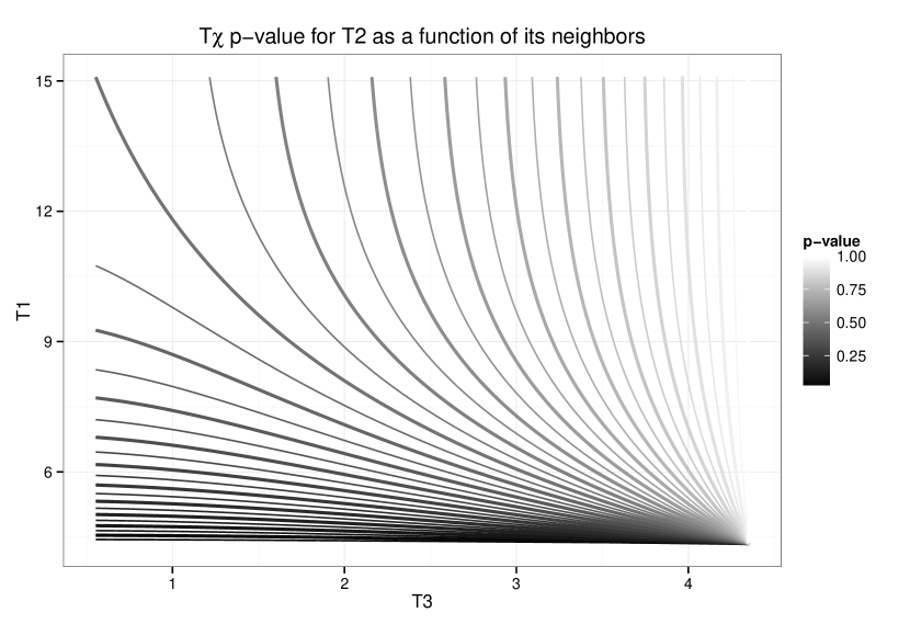
Figure 1: Contours of $T\chi$ $p$-value for $T_{2}$ as a function of its neighbors. Here $T_{2}\approx 4.35$ (corresponding to the 50% quantile of a $\chi^{2}_{5}$) is fixed and the upper and lower truncation limits vary.

Proposition 6.1 also yields some heuristic understanding. For example, we see explicitly the non-independence of the $T\chi$ statistics, but also note that in this case the dependency is only on neighboring statistics. Further, we see how the power for a given test depends on the values of the neighboring statistics. An example with groups of size 5 is plotted in Figure 1. This example considers a fixed value of $T_{2}$ and plots contours of the $p$-value for $T_{2}$ as a function of the neighboring statistics. It is apparent that when $T_{3}\to T_{2}$ (right side of plot), the $p$-value for $T_{2}$ will be large irrespective of $T_{1}$.

This motivates us to consider when a given nonnull $T_{i}$ is likely to have a close lower limit, since that scenario results in low power. Since a non-central $\chi^{2}_{k}(\lambda)$ with non-centrality parameter $\lambda$ has mean $k+\lambda$ and variance $2k+4\lambda$, we expect that the nonnull $T_{i}$ will be larger and have greater spread than the $T_{i}$ corresponding to null variables. Hence, if the true signal is sparse then the risk of having a nearby lower limit is mostly due to the bulk of null statistics. By upper bounding the largest null statistic, we get an idea of both when forward stepwise will select the nonnull variables first and when the worst case for power can be excluded. Using Lemma 1 of Laurent and Massart (2000), for $\epsilon>0$ if we define

$$x=-\log(1-(1-\epsilon)^{1/G})$$ (36)

then if all $T_{i}$ are null (central) we have

$$\mathbb{P}\left(\max_{1\leq i\leq G}T_{i}^{2}>k+2\sqrt{kx}+2x\right)<\epsilon.$$ (37)

Table 2 gives values of the upper bound $k+2\sqrt{kx}+2x$ as a function of $G$ and $k$, where there are $G$ null groups of equal size $k$ and error variance $\sigma^{2}=1$. For example, with $G=50$ groups of size $k=2$ the null $\chi^{2}_{k}$ statistics will all be below 27.28 with 99% probability and 21.35 with 90% probability.

Table 2: High probability upper bounds for central $\chi^{2}_{k}$ statistics corresponding noise variables. The left panel gives 99% bounds and the right panel 90%. This assumes $G$ noise groups of equal size $k$, groupwise orthogonality, and error variance $\sigma^{2}=1$.

	$k$
$G$	2	5	10	50
10	23.24	30.56	40.42	100.96
20	24.99	32.52	42.62	104.17
50	27.28	35.07	45.48	108.29
100	28.99	36.98	47.60	111.32
1000	34.61	43.19	54.47	120.99

	$k$
$G$	2	5	10	50
10	17.16	23.66	32.62	89.31
20	18.98	25.74	34.99	92.90
50	21.35	28.43	38.03	97.44
100	23.12	30.42	40.27	100.74
1000	28.88	36.85	47.46	111.11

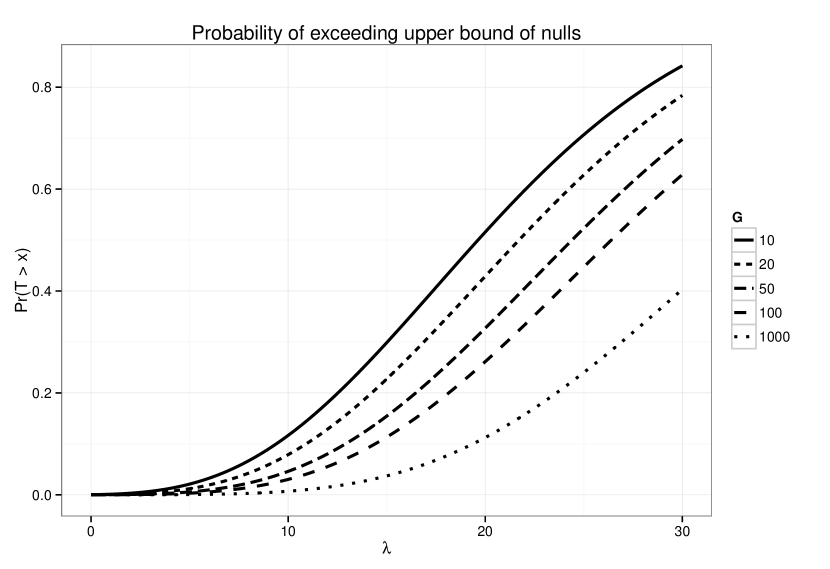
(a) Probability of a single nonnull exceeding the 90% theoretical bounds in Table 2.

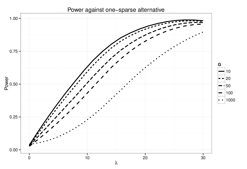
(b) Smoothed estimates of power functions for 1-sparse alternative and $G$ null variables.

Figure 2: Theoretical and empirical curves related to power against a one-sparse non-central $\chi^{2}_{5}$ with non-centrality parameter $\lambda$.

The power curves plotted in Fig 2 show this theoretical bound is likely more conservative than necessary. In fact, let us simplify a bit more by assuming orthogonal groups of size 1 (single columns), and a 1-sparse alternative with magnitude $(1+\delta)\sqrt{2\log(p)}$ for $\delta>0$. Then the standard tail bounds for Gaussian random variables imply that the $T\chi$ test is asymptotically equivalent to Bonferroni and hence asymptotically optimal for this alternative. This is discussed in Loftus and Taylor (2014) and a little more generally in Taylor, Loftus and Tibshirani (2015). The 1-sparse case with orthogonal groups of fixed, equal size follows similarly using tail bounds for $\chi^{2}$ random variables.

To translate between the non-centrality parameter $\lambda$ and a linear model coefficient, consider that when $y=X_{g}\beta_{g}+\epsilon$ and the expected column norms of $X_{g}$ scale like $\sqrt{n}$, then the non-centrality parameter for $T_{g}$ will be roughly equal to $\sqrt{n}\|\beta_{g}\|_{2}^{2}$ (under groupwise orthogonality).

Finally, when groups are not orthogonal, the greedy nature of forward stepwise will generally result in less power since part of the variation in $y$ due to $X_{g}$ may be regressed out at previous steps.

7 Simulations

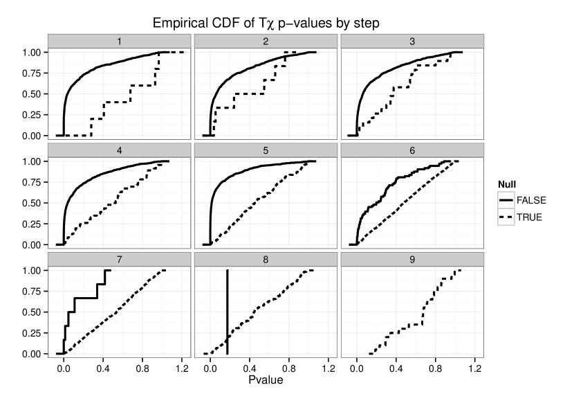
Figure 3: Empirical CDFs of $T\chi$ $p$-values plotted by step. Models chosen by BIC, with model size distribution described in Table 3. Design matrix had $n=100$ observations and $p=100$ variables in $G=50$ groups of size 2. The true sparsity is 5, nonzero entries of $\beta$ equal $\pm 2\sqrt{\log(G)/n}\approx\pm 0.4$. Dotted lines correspond to null variables and the solid, off-diagonal lines to signal variables.

To evaluate the $T\chi$ test when groupwise orthogonality does not hold, we conduct a simulation experiment with correlated Gaussian design matrices. In each of 1000 realizations forward stepwise is run with number of steps chosen by BIC. Table 3 summarizes the resulting model sizes and how many of the 5 nonnull variables were included.

Table 3: Size and composition of models chosen by BIC in the simulation described in Fig 3.

Model size	4	5	6	7	8	9
# Occurrences	4	42	511	328	95	20

# True signals included	3	4	5
# Occurrences	18	106	876

Fig 3 shows the empirical distributions of both null and nonnull $T\chi$ $p$-values plotted by the step the corresponding variable was added. Table 4 shows the power of rejecting at the $\alpha=0.05$ level also by step. Note that it was rare for nonnull variables to enter at later steps, so the observed power of 0 at step 8 is not too surprising.

Table 4: Empirical power for nonnull variables in the simulation described in Fig 3.

step	1	2	3	4	5	6	7	8
Power	0.532	0.470	0.454	0.521	0.641	0.315	0.500	0.000

References

- Akaike (1973) {binproceedings}[author] \bauthor\bsnmAkaike, \bfnmHirotugu\binitsH. (\byear1973). \btitleInformation Theory and an Extension of the Maximum. In \bbooktitleSecond International Symposium on Information Theory \bpages267–281. \endbibitem
- Chouldechova and Hastie (2015) {barticle}[author] \bauthor\bsnmChouldechova, \bfnmA.\binitsA. and \bauthor\bsnmHastie, \bfnmT.\binitsT. (\byear2015). \btitleGeneralized Additive Model Selection. \bjournalArXiv e-prints. \endbibitem
- Fithian, Sun and Taylor (2014) {barticle}[author] \bauthor\bsnmFithian, \bfnmWilliam\binitsW., \bauthor\bsnmSun, \bfnmDennis\binitsD. and \bauthor\bsnmTaylor, \bfnmJonathan\binitsJ. (\byear2014). \btitleOptimal inference after model selection. \bjournalarXiv preprint arXiv:1410.2597. \endbibitem
- Foster and George (1994) {barticle}[author] \bauthor\bsnmFoster, \bfnmDean P\binitsD. P. and \bauthor\bsnmGeorge, \bfnmEdward I\binitsE. I. (\byear1994). \btitleThe risk inflation criterion for multiple regression. \bjournalThe Annals of Statistics \bpages1947–1975. \endbibitem
- Gross, Taylor and Tibshirani (2015) {barticle}[author] \bauthor\bsnmGross, \bfnmS. M.\binitsS. M., \bauthor\bsnmTaylor, \bfnmJ.\binitsJ. and \bauthor\bsnmTibshirani, \bfnmR.\binitsR. (\byear2015). \btitleA Selective Approach to Internal Inference. \bjournalArXiv e-prints. \endbibitem
- Laurent and Massart (2000) {barticle}[author] \bauthor\bsnmLaurent, \bfnmBéatrice\binitsB. and \bauthor\bsnmMassart, \bfnmPascal\binitsP. (\byear2000). \btitleAdaptive estimation of a quadratic functional by model selection. \bjournalAnnals of Statistics \bpages1302–1338. \endbibitem
- Lee et al. (2015) {barticle}[author] \bauthor\bsnmLee, \bfnmJason D\binitsJ. D., \bauthor\bsnmSun, \bfnmDennis L\binitsD. L., \bauthor\bsnmSun, \bfnmYuekai\binitsY. and \bauthor\bsnmTaylor, \bfnmJonathan E\binitsJ. E. (\byear2015). \btitleExact post-selection inference with the lasso. \bjournalAnn. Statist. \bnoteTo appear. \endbibitem
- Lim and Hastie (2013) {barticle}[author] \bauthor\bsnmLim, \bfnmMichael\binitsM. and \bauthor\bsnmHastie, \bfnmTrevor\binitsT. (\byear2013). \btitleLearning interactions through hierarchical group-lasso regularization. \bjournalarXiv preprint arXiv:1308.2719. \endbibitem
- Lockhart et al. (2014) {barticle}[author] \bauthor\bsnmLockhart, \bfnmRichard\binitsR., \bauthor\bsnmTaylor, \bfnmJonathan\binitsJ., \bauthor\bsnmTibshirani, \bfnmRyan J.\binitsR. J. and \bauthor\bsnmTibshirani, \bfnmRobert\binitsR. (\byear2014). \btitleA significance test for the lasso. \bjournalAnn. Statist. \bvolume42 \bpages413–468. \bdoi10.1214/13-AOS1175 \endbibitem
- Loftus and Taylor (2014) {barticle}[author] \bauthor\bsnmLoftus, \bfnmJoshua R\binitsJ. R. and \bauthor\bsnmTaylor, \bfnmJonathan E\binitsJ. E. (\byear2014). \btitleA significance test for forward stepwise model selection. \bjournalarXiv preprint arXiv:1405.3920. \endbibitem
- University of Wisconsin Population Health Institute (2015) {bmisc}[author] \bauthor\bsnmUniversity of Wisconsin Population Health Institute (\byear2015). \btitleCalifornia County health rankings. \bhowpublishedhttp://www.countyhealthrankings.org. \bnoteAccessed: 2015-10-28. \endbibitem
- Schwarz et al. (1978) {barticle}[author] \bauthor\bsnmSchwarz, \bfnmGideon\binitsG. \betalet al. (\byear1978). \btitleEstimating the dimension of a model. \bjournalThe annals of statistics \bvolume6 \bpages461–464. \endbibitem
- Taylor, Loftus and Tibshirani (2015) {barticle}[author] \bauthor\bsnmTaylor, \bfnmJonathan E.\binitsJ. E., \bauthor\bsnmLoftus, \bfnmJoshua R.\binitsJ. R. and \bauthor\bsnmTibshirani, \bfnmRyan J.\binitsR. J. (\byear2015). \btitleTests in adaptive regression via the Kac-Rice formula. \bjournalAnn. Statist. \bnoteTo appear. \endbibitem
- Tibshirani et al. (2014) {barticle}[author] \bauthor\bsnmTibshirani, \bfnmR. J.\binitsR. J., \bauthor\bsnmTaylor, \bfnmJ.\binitsJ., \bauthor\bsnmLockhart, \bfnmR.\binitsR. and \bauthor\bsnmTibshirani, \bfnmR.\binitsR. (\byear2014). \btitleExact Post-Selection Inference for Sequential Regression Procedures. \bjournalArXiv e-prints. \endbibitem
- Tibshirani et al. (2015) {bmanual}[author] \bauthor\bsnmTibshirani, \bfnmRyan\binitsR., \bauthor\bsnmTibshirani, \bfnmRob\binitsR., \bauthor\bsnmTaylor, \bfnmJonathan\binitsJ., \bauthor\bsnmLoftus, \bfnmJoshua\binitsJ. and \bauthor\bsnmReid, \bfnmStephen\binitsS. (\byear2015). \btitleselectiveInference: Tools for Selective Inference \bnoteR package version 1.1.1. \endbibitem