Primordial trispectra and CMB spectral distortions

Abstract

We study the $TT\mu$ bispectrum, generated by correlations between Cosmic Microwave Background temperature (T) anisotropies and chemical potential ($\mu$) distortions, and we analyze its dependence on primordial local trispectrum parameters $g_{\rm NL}$ and $\tau_{\rm NL}$. We cross-check our results by comparing the full bispectrum calculation with the expectations from a general physical argument, based on predicting the shape of $\mu$-T correlations from the couplings between short and long perturbation modes induced by primordial non-Gaussianity. We show that both $g_{\rm NL}$ and $\tau_{\rm NL}$-parts of the primordial trispectrum source a non-vanishing $TT\mu$ signal, contrary to the $\mu\mu$ auto-correlation function, which is sensitive only to the $\tau_{\rm NL}$-component. A simple Fisher matrix-based forecast shows that a futuristic, cosmic-variance dominated experiment could in principle detect $g_{\rm NL}\sim 0.4$ and $\tau_{\rm NL}\sim 40$ using $TT\mu$.

IPMU15-0192

1 Introduction

Measurements of primordial non-Gaussianity (NG) are a powerful way to understand the physical processes which gave origin to primordial cosmological perturbations. They provide information about such processes which is complementary to what can be extracted from power spectrum alone. If we focus on inflationary scenarios, all relevant NG information is generally contained in the bispectrum (three-point function in Fourier space) and trispectrum (four-point function in Fourier space) of the primordial fluctuation field. Both the functional form (“shape”) and strength of these signals are model dependent, therefore constraints on different inflationary scenarios can be obtained by fitting their predicted bispectrum and trispectrum shapes to the data, and extracting the corresponding amplitude parameters $f_{\textrm{NL}}$ (for the bispectrum), $g_{\textrm{NL}}$ and $\tau_{\textrm{NL}}$ (for the trispectrum).

The first inflation-motivated primordial NG model to be considered in the literature [1, 2] was the so called “local model”, which is characterized by the following ansatz in real space:

$$\zeta(\mathbf{x})=\zeta^{\rm G}(\mathbf{x})+\frac{3}{5}f_{\textrm{NL}}\left(\zeta^{\rm G}(\mathbf{x})-\left\langle\zeta^{\rm G}(\mathbf{x})\right\rangle\right)^{2}+\frac{9}{25}g_{\textrm{NL}}\left(\zeta^{\rm G}(\mathbf{x})\right)^{3}\;,$$ (1.1)

where $\zeta$ is the primordial curvature perturbation field, $\zeta^{\rm G}$ is its Gaussian (G) part and the NG components are local functionals of the G part. One can also consider models in which $\zeta^{\rm G}$ is modulated by a second, uncorrelated, Gaussian field $\sigma$, giving rise to a “$\tau_{\textrm{NL}}$ trispectrum” [3]:

$$\zeta({\bf x})=\zeta^{\rm G}({\bf x})+\sqrt{\tau_{\textrm{NL}}}\sigma({\bf x})\zeta^{\rm G}({\bf x})\;.$$ (1.2)

As we just mentioned, different primordial models can generate a large variety of different bispectrum and trispectrum shapes, and to each of them correspond different NG amplitudes. The focus of this paper will however be specifically on local-type bispectra and trispectra, which are produced by a primordial curvature perturbation field expressed in the form above. 

Currently, the most stringent constraints on primordial NG come from Planck measurements of the Cosmic Microwave Background (CMB) temperature and polarization bispectra and trispectra [4, 5, 6]. For the local shape, they are $f_{\textrm{NL}}=2.5\pm 5.7$ (68 % CL), $g_{\textrm{NL}}=(-9.0\pm 7.7)\times 10^{4}$ (68 % CL) [6], $\tau_{\textrm{NL}}<2800$ (95 % CL) [4]. While being very tight, and representing, as emphasized in Planck papers, the highest precision test to date of the standard single-field slow-roll paradigm, these results by no mean rule out more complex multi-field models. In absence of a clear detection, if we want to convincingly discriminate between single and multi-field scenarios, it would in fact be necessary to find a test producing at least one order of magnitude, if not better, improvements in $f_{\textrm{NL}}$ error bars. This would probe a range of amplitudes which is at the level of the standard single-field slow-roll prediction, $f_{\textrm{NL}}\sim\epsilon$, where $\epsilon\sim 10^{-2}$ is the slow-roll parameter. Moreover, popular multi-field scenarios, such as the curvaton model, naturally predict a lower bound of order unity for $|f_{\textrm{NL}}|$, so that constraining this parameter to take much smaller values would effectively rule them out. Significant improvements in trispectrum constraints would also provide crucial information, allowing to further discriminate between competing scenarios for the origin of cosmic structures. In particular, sizable squeezed trispectra $g_{\textrm{NL}}$ and $\tau_{\textrm{NL}}$ can arise only within multi-field models of inflation. If there is a nonvanishing local bispectrum then there must be a trispectrum with $\tau_{\textrm{NL}}\geq(6f_{\rm NL}/5)^{2}$, according to the Suyama-Yamaguchi relation [7]. Moreover there are inflationary scenarios where the trispectrum has larger signal-to-noise than the bispectrum. For example, this is the case of some curvaton [8, 9] or other multi-field models [10, 11], where, for some parameter values, significant $g_{\textrm{NL}}$ and $\tau_{\textrm{NL}}$, respectively, can be generated along with a small $f_{\rm NL}$. Example of technically natural models where the trispectrum has larger signal-to-noise [12, 13, 14] do exist. This can happen also in multi-field models where the observed curvature perturbation is modulated by an uncorrelated field, such as those parametrized by Eq. (1.2). These models are characterized by a vanishing bispectrum, thus leaving the $\tau_{\textrm{NL}}$-trispectrum as the main NG signature. Planck has nearly saturated the maximum amount of information on NG parameters that can be extracted from CMB temperature and polarization. Even an ideal, cosmic variance dominated experiment, could not improve on current NG constraints by more than a factor $\sim 2-3$. It is then clear that, while CMB anisotropies have been the main driver for experimental NG studies up to now, we will have to turn to different observables in the future, if we hope to achieve the desired order of magnitude(s) leap.

A natural attempt, in this respect, is to look at Large Scale Structure statistics and forthcoming Euclid data [15]. Expectations of future improvements in this case rely at the moment mostly on measurements of scale-dependent halo bias in the 2-point function [16], but, even in the most optimistic picture, forecasted error bars are far from allowing to explore the $f_{\textrm{NL}}\ll 1$ regime we are ultimately interested in, as well as from producing order-of-magnitude improvements in trispectrum parameters.

If we look at more futuristic scenarios, three main approaches have been proposed to achieve the desired sensitivity on NG parameters. One is to look at the higher-order correlation functions of full-sky 21-cm radiation surveys, in the redshift range $30<z<100$ (e.g., [17, 18, 19, 20, 21, 22]). Another possibility is to study scale-dependent bias in future radio surveys probing high redshifts (e.g., [23, 24, 25, 26]). The third approach, which we focus on in this paper, was recently introduced in [27]. It consists in measuring cross-correlations between CMB chemical potential ($\mu$) spectral distortions, arising from dissipation of acoustic waves in the primordial photon-baryon plasma, and temperature anisotropies. As originally pointed out by the authors of [27], the $\mu T$ correlation probes the local bispectrum at wavenumbers $50\,{\rm Mpc}^{-1}\lesssim k\lesssim 10^{4}\,{\rm Mpc}^{-1}$, i.e. on scales which are unaccessible by CMB temperature or polarization anisotropies, or by any other cosmological probe, including future galaxy and 21-cm surveys. An ideal, cosmic-variance dominated experiment could extract a very large number of modes in this range of scales, allowing in principle constraints on $f_{\textrm{NL}}\lesssim 10^{-3}$. Moreover, it was also shown that, by the same reasoning, cosmic variance dominated $\mu\mu$ measurements could constrain $\tau_{\textrm{NL}}$ with an exquisite level of precision as well. These original findings have been followed by further studies from several groups, showing that $\mu T$ correlations could be used to study several other NG signatures besides standard local-type NG [27, 28, 29, 30, 31, 32, 33, 34, 35]. Recent $f_{\textrm{NL}}$ constraints with this technique were obtained in [36] using Planck data.

One interesting primordial NG parameter, that $\mu T$ and $\mu\mu$ correlations are unable to determine, is the $g_{\textrm{NL}}$ trispectrum amplitude. It can in fact be shown (see also Sec. 4) that $\mu\mu$ correlations are not sensitive to $g_{\textrm{NL}}$-type local NG. In this paper, we will point out that $g_{\textrm{NL}}$ can however still be measured by going beyond two-point correlations and using the $TT\mu$ bispectrum. We will then show that $TT\mu$ allows to measure not only $g_{\textrm{NL}}$, but also to extract additional information on $\tau_{\textrm{NL}}$. By a simple Fisher matrix forecast, we will finally conclude that $TT\mu$ bispectrum estimates could in principle allow a sensitivity $\Delta g_{\textrm{NL}}={\cal O}(0.1)$ in the ideal, cosmic variance dominated case. Such exquisite precision can be attained, as usual in this approach, thanks to the very large number of primordial bispectrum modes that are contained in the $TT\mu$ three-point function.

The plan of this paper is as follows: in Sec. 2 we start with a simplified calculation, aimed at putting in evidence the physical mechanism which produces the $g_{\textrm{NL}}$ and $\tau_{\textrm{NL}}$ dependencies in the $TT\mu$ bispectrum. We then perform the full calculation in Sec. 3, finding a nice agreement with the previous result, and show some $g_{\textrm{NL}}$ and $\tau_{\textrm{NL}}$ Fisher-based forecasts in Sec. 4, before reporting our conclusion in Sec. 5.

2 Preliminary calculation

Here we show a preliminary calculation of the $TT\mu$ signal, using a configuration space approach originally introduced in [34], where it is explained in detail. The idea is to estimate the expected correlations between $\mu$ and T via a short-long mode splitting of the primordial fluctuation field. We are in fact interested here in CMB distortions arising from dissipation of primordial perturbations on small scales. These will be proportional to the primordial small scale power. For Gaussian initial conditions, different small scale patches are uncorrelated, and the average distortion will be the same everywhere. If, however, we are in presence of NG initial conditions correlating large and small scales, such as local-type NG, the average small-scale power will vary from patch to patch, and it will be correlated with curvature fluctuations on large scales. We can thus infer the expected fluctuations in the $\mu$ (and $y$) distortions parameter by evaluating the contributions to small scale power, coming from correlations with long wavelength modes. In this framework, let us consider a NG primordial perturbation field, with non-zero $g_{\textrm{NL}}$, while keeping $f_{\textrm{NL}}=0$ and $\tau_{\textrm{NL}}=0$:

$$\zeta(\mathbf{x})=\zeta^{\rm G}(\mathbf{x})+\frac{9}{25}g_{\textrm{NL}}\left(\zeta^{\rm G}(\mathbf{x})\right)^{3}\;.$$ (2.1)

Let us split the curvature perturbation $\zeta^{\rm G}({\bf x})$ into short and long wavelength parts, $\zeta^{\rm G}({\bf x})=\zeta^{\rm G}_{S}({\bf x})+\zeta^{\rm G}_{L}({\bf x})$, and similarly for $\zeta({\bf x})$. Using this split into Eq. (2.1) we can read the corresponding short and long wavelength contributions to $\zeta({\bf x})$. The dominant terms are

$$\zeta({\bf x}) = \zeta_{S}({\bf x})+\zeta_{L}({\bf x})$$ (2.2)

$$= \zeta^{\rm G}_{S}({\bf x})+\zeta^{\rm G}_{L}({\bf x})+\frac{27}{25}g_{\rm NL}\zeta^{\rm G}_{S}({\bf x})\left(\zeta^{\rm G}_{L}({\bf x})\right)^{2}\,,$$

so that the small-scale curvature perturbation modulated by the long-wavelength modes is given by

$$\zeta_{S}({\bf x})=\zeta^{\rm G}_{S}({\bf x})\left[1+\frac{27}{25}g_{\rm NL}\left(\zeta^{\rm G}_{L}({\bf x})\right)^{2}\right]\,.$$ (2.3)

The fractional change in small-scale power due to the long-wavelength mode is therefore

$$\frac{\delta\langle\zeta^{2}\rangle}{\langle\zeta^{2}\rangle}\simeq\frac{\delta\mu}{\mu}\simeq\frac{54}{25}g_{\rm NL}\left(\zeta^{\rm G}_{L}({\bf x})\right)^{2}\,.$$ (2.4)

As written in the second equality the fractional change in small-scale power determines the fractional change in the $\mu$ type distortions, since the average $\mu$ distortions are given by

$$\langle\mu\rangle\simeq\int d\ln k\,\Delta^{2}_{\zeta}(k)\,F(k)\,,$$ (2.5)

where $\Delta^{2}_{\zeta}(k)$ is the power spectrum of the primordial curvature perturbations. $F(k)$ is the $k$-space window function denoted as $W(k)$ in [34]: $F(k)\simeq(9/4)[e^{-2k^{2}/k^{2}_{D}(z_{i})}-e^{-2k^{2}/k^{2}_{D}(z_{f})}]$ where $k_{D}(z)$ is the damping scale, and we need to evaluate the difference respectively at redshifts $z_{i}\sim 2\times 10^{6}$ and $z_{f}\sim 5\times 10^{4}$, defining the $\mu$-distortion era. Such redshifts correspond to diffusion scales $k_{i}\equiv k_{D}(z_{i})\simeq 12000\,{\rm Mpc}^{-1}$ and $k_{f}\equiv k_{D}(z_{f})\simeq 46\,{\rm Mpc}^{-1}$ [37, 38, 39, 40]. Let us now compute the $TT\mu$ bispectrum induced by the $g_{\rm NL}$ type trispectrum

$$\left\langle\frac{\delta T_{1}}{T}\frac{\delta T_{2}}{T}\frac{\delta\mu_{3}}{\mu}\right\rangle \simeq \frac{54}{25}g_{\rm NL}\left\langle\frac{\zeta_{1}}{5}\frac{\zeta_{2}}{5}\left(\zeta^{\rm G}_{L3}\right)^{2}\right\rangle$$ (2.6)

$$= 108\,g_{\rm NL}\left\langle\frac{\delta T_{1}}{T}\frac{\delta T_{3}}{T}\right\rangle\left\langle\frac{\delta T_{2}}{T}\frac{\delta T_{3}}{T}\right\rangle\,.$$

In Eq. (2.6) the indices $1,2,3$ refer to three different positions on last-scattering surface (or, by means of an angular projection from the last-scattering surface, they label three different directions in the sky). Also, in writing Eq. (2.6) we have used that the large-angle temperature fluctuation is given by $\delta T/T\simeq-\zeta/5$ (in the Sachs-Wolfe (SW) approximation).

The equation above describes correlation between $\delta T/T$ and the fractional change in $\mu$-distortions, $\delta\mu/\mu$. If we want to work with $\mu$-fluctuations instead, we simply have to multiply Eq. (2.6) by the average $\mu$ distortions, Eq. (2.5). In the case of a scale invariant spectrum of primordial curvature perturbations with $\Delta^{2}_{\zeta}(k)=A_{S}$, $\langle\mu\rangle\simeq(9/4)A_{S}\ln(k_{i}/k_{f})$, this yields

$$b_{\ell_{1}\ell_{2}\ell_{3}}^{TT\mu}\simeq 108\,g_{\rm NL}\,\frac{9}{4}A_{S}\ln\left(\frac{k_{i}}{k_{f}}\right)C_{\ell_{1}}^{TT}C_{\ell_{2}}^{TT}\,,$$ (2.7)

where we have moved to $\ell$ space by the harmonic transformation: $\left\langle\frac{\delta T_{1}}{T}\frac{\delta T_{2}}{T}\right\rangle\to C_{\ell_{1}}^{TT}$ and $\left\langle\frac{\delta T_{1}}{T}\frac{\delta T_{2}}{T}\delta\mu_{3}\right\rangle\to b_{\ell_{1}\ell_{2}\ell_{3}}^{TT\mu}$, with $C_{\ell}^{TT}$ and $b_{\ell_{1}\ell_{2}\ell_{3}}^{TT\mu}$ denoting the angular power spectrum and bispectrum (3.19), respectively.

The $TT\mu$ bispectrum induced by $\tau_{\rm NL}$-like NG can be computed in a similar way. Starting from Eq. (1.2), where the small-scale curvature perturbation $\zeta^{\rm G}({\bf x})$ is modulated by the large-scale field $\sigma({\bf x})$, we find (at leading order and up to disconnected parts)

$$\frac{\delta\langle\zeta^{2}\rangle}{\langle\zeta^{2}\rangle}\simeq\frac{\delta\mu}{\mu}\simeq 2\sqrt{\tau_{\rm NL}}\sigma({\bf x})\,.$$ (2.8)

Notice that, following the conventional definition of $\tau_{\rm NL}$, in Eq. (1.2) $\sigma({\bf x})$ is normalized in such a way that it has equal power spectrum as $\zeta^{\rm G}({\bf x})$, $\langle\sigma^{2}\rangle=\langle(\zeta^{\rm G})^{2}\rangle$. Therefore

$$\left\langle\frac{\delta T_{1}}{T}\frac{\delta T_{2}}{T}\frac{\delta\mu_{3}}{\mu}\right\rangle \simeq 2\left\langle\frac{\zeta_{1}^{\rm G}}{5}\frac{\zeta_{2}^{\rm G}}{5}\left[1+\sqrt{\tau_{\textrm{NL}}}(\sigma_{1}+\sigma_{2})\right]\sqrt{\tau_{\textrm{NL}}}\sigma_{3}\frac{}{}\right\rangle$$ (2.9)

$$= 50\tau_{\textrm{NL}}\left[\left\langle\frac{\delta T_{1}}{T}\frac{\delta T_{2}}{T}\right\rangle\left\langle\frac{\delta T_{2}}{T}\frac{\delta T_{3}}{T}\right\rangle+(1\leftrightarrow 2)\right]\,.$$

Finally, multiplying by the average $\mu$ distortion, we obtain the harmonic-space expression of $\left\langle\frac{\delta T_{1}}{T}\frac{\delta T_{2}}{T}\delta\mu_{3}\right\rangle$

$$b_{\ell_{1}\ell_{2}\ell_{3}}^{TT\mu}\simeq 50\,\tau_{\rm NL}\,\frac{9}{4}A_{S}\ln\left(\frac{k_{i}}{k_{f}}\right)\left[C_{\ell_{1}}^{TT}+C_{\ell_{2}}^{TT}\right]C_{\ell_{3}}^{TT}\,.$$ (2.10)

In the next section, we will show how these results very nicely match a full detailed computation.

3 The $TT\mu$ bispectrum

After the warm up in the previous section, we are now ready to perform a full computation of the $TT\mu$ three-point function, arising from both $g_{\textrm{NL}}$ and $\tau_{\textrm{NL}}$ contributions. At the end of the section, we will find excellent agreement between the full and simplified treatments. Let us note, before starting our calculation, that $y$-type distortions could have been considered as well, and the $TTy$ bispectrum would produce contributions to the signal coming from a different range of scales. The authors of [27] originally did not include y-contributions in their study of two-point correlations. This was based on the fact that primordial $Ty$ and $yy$ signals would be affected by large contaminations coming from late-time Compton-y signals. It was however argued in [34] that $yT$ primordial NG signatures could in principle be used to disentangle the high-redshift and low-redshift components. It remains anyway clear that $\mu$-T correlations provide the cleanest signal. We will thus focus here only on $TT\mu$, leaving issues related to $TTy$ contributions for future work.

CMB temperature anisotropies are linked, at first order, to primordial curvature perturbations via the usual formula:

$$a_{\ell m}^{T}=4\pi i^{\ell}\int\frac{d^{3}{\bf k}}{(2\pi)^{3}}{\cal T}_{\ell}(k)\zeta_{\bf k}Y_{\ell m}^{*}(\hat{\bf k})\;,$$ (3.1)

where ${\cal T}_{\ell}(k)$ indicates the radiation transfer function, and $\zeta_{\bf k}$ is the primordial curvature perturbation.

The $\mu$ spectral distortion parameter from dissipation of acoustic fluctuations can instead be obtained as (e.g. [41, 42, 43, 44, 45, 46, 47, 48, 49, 50, 37, 38, 39, 40, 27, 28, 36]):

$$a_{\ell m}^{\mu}=4\pi(-i)^{\ell}\left[\prod_{n=1}^{2}\int\frac{d^{3}{\bf k}_{n}}{(2\pi)^{3}}\zeta_{{\bf k}_{n}}\right]\int d^{3}{\bf k}_{3}\delta^{(3)}\left({\bf k}_{1}+{\bf k}_{2}+{\bf k}_{3}\right)Y_{\ell m}^{*}(\hat{\bf k}_{3})j_{\ell}(k_{3}x_{\rm ls})f(k_{1},k_{2},k_{3})\;,$$ (3.2)

where $x_{\rm ls}$ is the conformal distance to the last scattering surface and:

$$f(k_{1},k_{2},k_{3})\simeq\frac{9}{4}W\left(\frac{k_{3}}{k_{s}}\right)\left[e^{-(k_{1}^{2}+k_{2}^{2})/k_{D}^{2}(z)}\right]_{f}^{i}\;.$$ (3.3)

In the last formula, $W(k/k_{s})$ is a window function selecting the range of scales $k/k_{s}\lesssim 1$ for acoustic wave dissipation, and the square bracket takes the difference between the quantities at $z_{i}\sim 2\times 10^{6}$ and $z_{f}\sim 5\times 10^{4}$, namely, $[g(z)]_{f}^{i}\equiv g(z_{i})-g(z_{f})$. The $\langle a_{\ell_{1}m_{1}}^{T}a_{\ell_{2}m_{2}}^{T}a_{\ell_{3}m_{3}}^{\mu}\rangle$ bispectrum can now be written as:

$$\Braket{a_{\ell_{1}m_{1}}^{T}a_{\ell_{2}m_{2}}^{T}a_{\ell_{3}m_{3}}^{\mu}} = \left[\prod_{n=1}^{2}4\pi i^{\ell_{n}}\int\frac{d^{3}{\bf k}_{n}}{(2\pi)^{3}}{\cal T}_{\ell_{n}}(k_{n})Y_{\ell_{n}m_{n}}^{*}(\hat{\bf k}_{n})\right]$$ (3.4)

$$4\pi(-i)^{\ell_{3}}\left[\prod_{n=1}^{2}\int\frac{d^{3}{\bf K}_{n}}{(2\pi)^{3}}\right]\int d^{3}{\bf K}_{3}\delta^{(3)}\left({\bf K}_{1}+{\bf K}_{2}+{\bf K}_{3}\right)$$

$$Y_{\ell_{3}m_{3}}^{*}(\hat{\bf K}_{3})j_{\ell_{3}}(K_{3}x_{\rm ls})f(K_{1},K_{2},K_{3})\Braket{\zeta_{{\bf k}_{1}}\zeta_{{\bf k}_{2}}\zeta_{{\bf K}_{1}}\zeta_{{\bf K}_{2}}}\,.$$

3.1 $g_{\textrm{NL}}$ contributions

The $g_{\textrm{NL}}$-type trispectrum is given as

$$\Braket{\zeta_{{\bf k}_{1}}\zeta_{{\bf k}_{2}}\zeta_{{\bf K}_{1}}\zeta_{{\bf K}_{2}}}=(2\pi)^{3}\delta^{(3)}\left({\bf k}_{1}+{\bf k}_{2}+{\bf K}_{1}+{\bf K}_{2}\right)T(k_{1},k_{2},K_{1},K_{2})\;,$$ (3.5)

with

$$T(k_{1},k_{2},K_{1},K_{2})=\frac{54}{25}g_{\textrm{NL}}\left[P(k_{1})P(k_{2})P(K_{1})+(3~{}{\rm perm})\right]~{}.$$ (3.6)

Substituting this into Eq. (3.4), it is possible to arrive at the following expression

$$\Braket{a_{\ell_{1}m_{1}}^{T}a_{\ell_{2}m_{2}}^{T}a_{\ell_{3}m_{3}}^{\mu}} = \left[\prod_{n=1}^{2}4\pi i^{\ell_{n}}\int\frac{d^{3}{\bf k}_{n}}{(2\pi)^{3}}{\cal T}_{\ell_{n}}(k_{n})Y_{\ell_{n}m_{n}}^{*}(\hat{\bf k}_{n})\right]$$ (3.14)

$$4\pi(-i)^{\ell_{3}}\left[\prod_{n=1}^{2}\int\frac{d^{3}{\bf K}_{n}}{(2\pi)^{3}}\right]\int d^{3}{\bf K}_{3}$$

$$8\int_{0}^{\infty}y^{2}dy\left[\prod_{n=1}^{3}\sum_{L_{n}M_{n}}j_{L_{n}}(K_{n}y)Y_{L_{n}M_{n}}^{*}(\hat{\bf K}_{n})\right]$$

$$(-1)^{\frac{L_{1}+L_{2}+L_{3}}{2}}h_{L_{1}L_{2}L_{3}}\left(\begin{array}[]{ccc}L_{1}&L_{2}&L_{3}\\ M_{1}&M_{2}&M_{3}\end{array}\right)$$

$$Y_{\ell_{3}m_{3}}^{*}(\hat{\bf K}_{3})j_{\ell_{3}}(K_{3}x_{\rm ls})f(K_{1},K_{2},K_{3})(2\pi)^{3}T(k_{1},k_{2},K_{1},K_{2})$$

$$2^{5}\pi\int_{0}^{\infty}r^{2}dr\left[\prod_{n=1}^{2}\sum_{l_{n}^{\prime}m_{n}^{\prime}}j_{l_{n}^{\prime}}(k_{n}r)Y_{l_{n}^{\prime}m_{n}^{\prime}}^{*}(\hat{\bf k}_{n})\sum_{L_{n}^{\prime}M_{n}^{\prime}}j_{L_{n}^{\prime}}(K_{n}r)Y_{L_{n}^{\prime}M_{n}^{\prime}}^{*}(\hat{\bf K}_{n})\right]$$

$$(-1)^{\frac{l_{1}^{\prime}+l_{2}^{\prime}+L_{1}^{\prime}+L_{2}^{\prime}}{2}}\sum_{L^{\prime}M^{\prime}}(-1)^{M^{\prime}}h_{l_{1}^{\prime}l_{2}^{\prime}L^{\prime}}h_{L_{1}^{\prime}L_{2}^{\prime}L^{\prime}}$$

$$\left(\begin{array}[]{ccc}l_{1}^{\prime}&l_{2}^{\prime}&L^{\prime}\\ m_{1}^{\prime}&m_{2}^{\prime}&M^{\prime}\end{array}\right)\left(\begin{array}[]{ccc}L_{1}^{\prime}&L_{2}^{\prime}&L^{\prime}\\ M_{1}^{\prime}&M_{2}^{\prime}&-M^{\prime}\end{array}\right)\;,$$

where $\left(\begin{array}[]{ccc}\ell_{1}&\ell_{2}&\ell_{3}\\ m_{1}&m_{2}&m_{3}\end{array}\right)$ are Wigner-3j symbols, and we defined:

$$h_{l_{1}l_{2}l_{3}}\equiv\sqrt{\frac{(2l_{1}+1)(2l_{2}+1)(2l_{3}+1)}{4\pi}}\left(\begin{array}[]{ccc}l_{1}&l_{2}&l_{3}\\ 0&0&0\end{array}\right)\;.\\$$ (3.15)

In order to go from Eq. (3.4) to Eq. (3.14) we used integral representations for the Dirac delta functions, expanding plane waves in spherical harmonics:

$$e^{i{\bf k}\cdot{\bf x}}=\sum_{LM}4\pi i^{L}j_{L}(kx)Y_{LM}(\hat{\bf k})Y_{LM}^{*}(\hat{\bf x})\;,$$ (3.16)

and used the Gaunt integral representation for integrals of products of three spherical harmonics. We can now use the orthonormality relation for spherical harmonics:

$$\int d^{2}\hat{\bf n}Y_{\ell_{1}m_{1}}(\hat{\bf n})Y_{\ell_{2}m_{2}}^{*}(\hat{\bf n})=\delta_{\ell_{1},\ell_{2}}\delta_{m_{1},m_{2}}\;,$$ (3.17)

and the completeness of Wigner-3j symbols:

$$\frac{\delta_{l_{3},l_{3}^{\prime}}\delta_{m_{3},m_{3}^{\prime}}}{(2l_{3}+1)}=\sum_{m_{1}m_{2}}\left(\begin{array}[]{ccc}l_{1}&l_{2}&l_{3}\\ m_{1}&m_{2}&m_{3}\end{array}\right)\left(\begin{array}[]{ccc}l_{1}&l_{2}&l_{3}^{\prime}\\ m_{1}&m_{2}&m_{3}^{\prime}\end{array}\right)\;,$$ (3.18)

to further simplify Eq. (3.14) into:

$$\Braket{a_{\ell_{1}m_{1}}^{T}a_{\ell_{2}m_{2}}^{T}a_{\ell_{3}m_{3}}^{\mu}}=h_{\ell_{1}\ell_{2}\ell_{3}}\left(\begin{array}[]{ccc}\ell_{1}&\ell_{2}&\ell_{3}\\ m_{1}&m_{2}&m_{3}\end{array}\right)b_{\ell_{1}\ell_{2}\ell_{3}}^{TT\mu}\;,$$ (3.19)

where we have defined the reduced bispectrum:

$$b_{\ell_{1}\ell_{2}\ell_{3}}^{TT\mu} = \int_{0}^{\infty}r^{2}dr\int_{0}^{\infty}y^{2}dy\,\frac{2}{\pi}\int_{0}^{\infty}k_{1}^{2}dk_{1}{\cal T}_{\ell_{1}}(k_{1})j_{\ell_{1}}(k_{1}r)\,\frac{2}{\pi}\int_{0}^{\infty}k_{2}^{2}dk_{2}{\cal T}_{\ell_{2}}(k_{2})j_{\ell_{2}}(k_{2}r)\,$$ (3.20)

$$\sum_{L_{1}L_{2}}\frac{h_{L_{1}L_{2}\ell_{3}}^{2}}{2\ell_{3}+1}\frac{2}{\pi}\int_{0}^{\infty}K_{1}^{2}dK_{1}j_{L_{1}}(K_{1}y)j_{L_{1}}(K_{1}r)\,\frac{2}{\pi}\int_{0}^{\infty}K_{2}^{2}dK_{2}j_{L_{2}}(K_{2}y)j_{L_{2}}(K_{2}r)\,$$

$$\frac{2}{\pi}\int_{0}^{\infty}K_{3}^{2}dK_{3}j_{\ell_{3}}(K_{3}x_{\rm ls})j_{\ell_{3}}(K_{3}y)f(K_{1},K_{2},K_{3})T(k_{1},k_{2},K_{1},K_{2})\;.$$

The factorization in Eq. (3.19) is, as usual in this type of calculations (see e.g., [51]), a direct consequence of the rotational invariance properties of the CMB sky. All physical information is contained in the reduced bispectrum defined in Eq. (3.20). Up to this point, we performed an exact calculation. In order to make Eq. (3.20) feasible for numerical evaluation, we now simplify it by using the following approximation:

$$\int_{0}^{\infty}K_{3}^{2}dK_{3}j_{\ell_{3}}(K_{3}x_{\rm ls})j_{\ell_{3}}(K_{3}y)W\left(\frac{K_{3}}{k_{s}}\right) \simeq \int_{0}^{\infty}K_{3}^{2}dK_{3}j_{\ell_{3}}(K_{3}x_{\rm ls})j_{\ell_{3}}(K_{3}y)$$ (3.21)

$$= \frac{\pi\delta(y-x_{\rm ls})}{2x_{\rm ls}^{2}}~{}.$$

This is justified by the fact that the spherical Bessel function $j_{\ell}(kx)$ is peaked for $\ell\sim kx$, and decays rapidly afterwards. We can regard $k_{s}$ in the argument of the window function, $W(K_{3}/k_{s})$, as the damping scale at recombination $k_{D}(z_{*}\simeq 1100)$ [36], and the integral then converges to very high accuracy well before the $K_{3}\sim k_{D}(z_{*})$ cutoff, as long as $\ell_{3}\ll k_{D}(z_{*})x_{\rm ls}\simeq 2000$. This condition will always be verified in the following, since in our forecasts we will take $\ell_{1}=\ell_{2}=\ell_{3}=1000$ as our maximum value. The last equality in Eq. (3.21) expresses the completeness of spherical Bessel functions. Plugging Eq. (3.21) and the $g_{\textrm{NL}}$ trispectrum formula (3.6) into Eq. (3.20) finally yields:

$$b_{\ell_{1}\ell_{2}\ell_{3}}^{TT\mu} \simeq \frac{54}{25}g_{\textrm{NL}}\sum_{L_{1}L_{2}}\frac{h_{L_{1}L_{2}\ell_{3}}^{2}}{2\ell_{3}+1}\int_{0}^{\infty}r^{2}dr$$ (3.22)

$$\left[\beta_{\ell_{1}}^{T}(r)\beta_{\ell_{2}}^{T}(r)\beta_{L_{1}}^{\mu}(r,z)\alpha_{L_{2}}^{\mu}(r,z)+\beta_{\ell_{1}}^{T}(r)\beta_{\ell_{2}}^{T}(r)\alpha_{L_{1}}^{\mu}(r,z)\beta_{L_{2}}^{\mu}(r,z)\right.$$

$$\left.+\beta_{\ell_{1}}^{T}(r)\alpha_{\ell_{2}}^{T}(r)\beta_{L_{1}}^{\mu}(r,z)\beta_{L_{2}}^{\mu}(r,z)+\alpha_{\ell_{1}}^{T}(r)\beta_{\ell_{2}}^{T}(r)\beta_{L_{1}}^{\mu}(r,z)\beta_{L_{2}}^{\mu}(r,z)\right]_{f}^{i}~{},$$

where we have defined:

$$\alpha_{\ell}^{T}(r) \equiv \frac{2}{\pi}\int_{0}^{\infty}k^{2}dk{\cal T}_{\ell}(k)j_{\ell}(kr)~{},$$ (3.23)

$$\alpha_{\ell}^{\mu}(r,z) \equiv \frac{3}{\pi}\int_{0}^{\infty}k^{2}dkj_{\ell}(kx_{\rm ls})j_{\ell}(kr)e^{-k^{2}/k_{D}^{2}(z)}~{},$$ (3.24)

$$\beta_{\ell}^{T}(r) \equiv \frac{2}{\pi}\int_{0}^{\infty}k^{2}dkP(k){\cal T}_{\ell}(k)j_{\ell}(kr)~{},$$ (3.25)

$$\beta_{\ell}^{\mu}(r,z) \equiv \frac{3}{\pi}\int_{0}^{\infty}k^{2}dkP(k)j_{\ell}(kx_{\rm ls})j_{\ell}(kr)e^{-k^{2}/k_{D}^{2}(z)}.$$ (3.26)

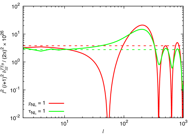
Figure 1: $TT\mu$ for $g_{\textrm{NL}}=1$ and $\tau_{\textrm{NL}}=1$. The solid and dashed lines describe the results including full transfer function (computed from Eqs. (3.32) and (3.38)) and those in the SW limit (computed from Eqs. (3.33) and (3.41)), respectively. As expected, the SW approximation agrees well with the full calculation on very small $\ell$’s.

Let us now consider a scale-invariant primordial power spectrum, $P(k)=2\pi^{2}A_{S}k^{-3}$. Using again asymptotic properties and the completeness relation for spherical Bessel functions, as well as keeping into account the $k_{D}$ cutoff in Eqs. (3.24) and (3.26), we can approximately evaluate $\alpha_{\ell}^{\mu}$ and $\beta_{\ell}^{\mu}$ as follows:

$$\alpha_{L}^{\mu}(r,z) \approx \begin{cases}\frac{3\delta(r-x_{\rm ls})}{2x_{\rm ls}^{2}}&:L\lesssim L_{D}(z)\\ 0&:L\gtrsim L_{D}(z)\end{cases}~{},$$ (3.27)

$$\beta_{L}^{\mu}(x_{\rm ls},z) \approx \begin{cases}\frac{3\pi A_{S}}{L(L+1)}&:L\lesssim L_{D}(z)\\ 0&:L\gtrsim L_{D}(z)\end{cases}\;,$$ (3.28)

where we have defined $L_{D}(z)\equiv k_{D}(z)x_{\rm ls}$. In Eq. (3.22) we can thus operate the replacement

$$\sum_{L_{1},L_{2}=0}^{\infty}\rightarrow\sum_{L_{1},L_{2}=L_{f}}^{L_{i}}\;,$$ (3.29)

with $L_{f}\equiv k_{f}x_{\rm ls}\sim 10^{5}$ and $L_{i}\equiv k_{i}x_{\rm ls}\sim 10^{8}$. We can then see that $L_{1},L_{2}$ are very large and $L_{1},L_{2}\gg\ell_{3}$ in the sum. In light of this, and using the Stirling approximation to evaluate the Wigner symbols, we can get the following asymptotic formula:

$$h_{l_{1}l_{2}l_{3}}^{2}\simeq\frac{2l_{1}}{\pi^{2}}\;,$$ (3.30)

where we assume $l_{1}\simeq l_{2}$, in virtue of the triangle inequality, imposing $|l_{1}-l_{2}|\leq l_{3}\leq l_{1}+l_{2}$, and of the condition $l_{1},l_{2}\gg l_{3}$.

We tested the approximation (3.30) by comparing $h_{l_{1}l_{2}l_{3}}^{2}$ computed numerically with $2l_{1}/\pi^{2}$, for $l_{1}\sim 1000$, and found that the error it introduces is $\sim 20\%$, which is completely reasonable for the order of magnitude Fisher forecasts in the next section. We can then operate the further replacement:

$$\sum_{L_{1},L_{2}=L_{f}}^{L_{i}}\frac{h_{L_{1}L_{2}\ell_{3}}^{2}}{2\ell_{3}+1}\simeq\sum_{L_{1},L_{2}=L_{f}}^{L_{i}}\frac{2L_{1}}{\pi^{2}}\delta_{L_{1},L_{2}}\;.$$ (3.31)

After substituting Eqs. (3.27) and (3.28) into Eq. (3.22), keeping the leading order terms in the sum over $L_{1}$, and evaluating the sum via integration, we finally arrive at the expression:

$$b_{\ell_{1}\ell_{2}\ell_{3}}^{TT\mu}\simeq\frac{972}{25\pi}g_{\textrm{NL}}A_{S}\ln\left(\frac{k_{i}}{k_{f}}\right)\beta_{\ell_{1}}^{T}(x_{\rm ls})\beta_{\ell_{2}}^{T}(x_{\rm ls})~{}.$$ (3.32)

If we take the Sachs-Wolfe (SW) limit, ${\cal T}_{\ell}(k)\to-\frac{1}{5}j_{\ell}(kx_{\rm ls})$, we can further simplify this into the following analytical expression:

$$b_{\ell_{1}\ell_{2}\ell_{3}}^{TT\mu,\rm SW}\simeq\frac{972}{\pi}g_{\textrm{NL}}A_{S}\ln\left(\frac{k_{i}}{k_{f}}\right)C_{\ell_{1},\rm SW}^{TT}C_{\ell_{2},\rm SW}^{TT}\;,$$ (3.33)

where $C_{\ell,\rm SW}^{TT}=\frac{2\pi A_{S}}{25\ell(\ell+1)}$. This is consistent with our expectation in Eq. (2.7) (the $4/\pi$ difference is simply due to the approximation in Eq. (3.30)).

3.2 $\tau_{\textrm{NL}}$ contributions

The $TT\mu$ signal arising from a primordial local $\tau_{\textrm{NL}}$-trispectrum can be computed in similar fashion as we did for the $g_{\textrm{NL}}$ part. Starting from Eq. (3.4), we include the $\tau_{\textrm{NL}}$ shape:

$$\Braket{\zeta_{{\bf k}_{1}}\zeta_{{\bf k}_{2}}\zeta_{{\bf K}_{1}}\zeta_{{\bf K}_{2}}}=(2\pi)^{3}\delta^{(3)}\left({\bf k}_{1}+{\bf k}_{2}+{\bf K}_{1}+{\bf K}_{2}\right)\tau_{\textrm{NL}}\left[P(k_{1})P(K_{1})P(k_{12})+(11~{}{\rm perm})\right]~{},$$ (3.34)

where $k_{12}\equiv|{\bf k}_{1}+{\bf k}_{2}|$. We then take into account the fact that the filters $f(K_{1},K_{2},K_{3})$ select configurations for which $K_{1}\simeq K_{2}\gg K_{12}$. This allows to write:

$$\Braket{\zeta_{{\bf k}_{1}}\zeta_{{\bf k}_{2}}\zeta_{{\bf K}_{1}}\zeta_{{\bf K}_{2}}} \simeq (2\pi)^{3}\int d^{3}{\bf k}\delta^{(3)}\left({\bf k}_{1}+{\bf k}_{2}+{\bf k}\right)\delta^{(3)}\left({\bf K}_{1}+{\bf K}_{2}-{\bf k}\right)t_{K_{1}K_{2}}^{k_{1}k_{2}}(k)~{},$$ (3.35)

$$t_{K_{1}K_{2}}^{k_{1}k_{2}}(k) \equiv \tau_{\textrm{NL}}\left[P(k_{1})P(K_{1})+P(k_{1})P(K_{2})+P(k_{2})P(K_{1})+P(k_{2})P(K_{2})\right]P(k)~{}.$$

Using the expansions and properties which lead from Eq. (3.14) to Eq. (3.20), we arrive at:

$$b_{\ell_{1}\ell_{2}\ell_{3}}^{TT\mu} = \frac{8}{\pi^{6}}\int_{0}^{\infty}r^{2}dr\int_{0}^{\infty}k_{1}^{2}dk_{1}{\cal T}_{\ell_{1}}(k_{1})j_{\ell_{1}}(k_{1}r)\int_{0}^{\infty}k_{2}^{2}dk_{2}{\cal T}_{\ell_{2}}(k_{2})j_{\ell_{2}}(k_{2}r)$$ (3.36)

$$\int_{0}^{\infty}K_{1}^{2}dK_{1}\int_{0}^{\infty}K_{2}^{2}dK_{2}\int_{0}^{\infty}K_{3}^{2}dK_{3}j_{\ell_{3}}(K_{3}x_{\rm ls})j_{\ell_{3}}(K_{3}r)$$

$$\int_{0}^{\infty}y^{2}dyj_{0}(K_{1}y)j_{0}(K_{2}y)j_{0}(K_{3}y)f(K_{1},K_{2},K_{3})t_{K_{1}K_{2}}^{k_{1}k_{2}}(K_{3})\;.$$

In the limit $K_{1}\sim K_{2}\gg K_{3}$, we have $j_{0}(K_{3}y)\rightarrow 1$, and:

$$\int_{0}^{\infty}y^{2}dyj_{0}(K_{1}y)j_{0}(K_{2}y)j_{0}(K_{3}y)\simeq\frac{\pi\delta(K_{1}-K_{2})}{2K_{1}^{2}}~{}.$$ (3.37)

With this approximation we can write

$$b_{\ell_{1}\ell_{2}\ell_{3}}^{TT\mu} \simeq \frac{9}{2}\tau_{\textrm{NL}}A_{S}\ln\left(\frac{k_{i}}{k_{f}}\right)\int_{0}^{\infty}r^{2}dr\left[\alpha_{\ell_{1}}^{T}(r)\beta_{\ell_{2}}^{T}(r)+\beta_{\ell_{1}}^{T}(r)\alpha_{\ell_{2}}^{T}(r)\right]\omega_{\ell_{3}}(r)~{},$$ (3.38)

where

$$\omega_{\ell}(r)\equiv\frac{2}{\pi}\int_{0}^{\infty}k^{2}dkP(k)j_{\ell}(kx_{\rm ls})j_{\ell}(kr)W\left(\frac{k}{k_{s}}\right).$$ (3.39)

In the SW limit for $\alpha_{\ell}^{T}$ and $\beta_{\ell}^{T}$, and approximating $\omega_{\ell_{3}}(x_{\rm ls})$, for $\ell_{3}\ll k_{s}x_{\rm ls}\simeq 2000$, in the following way:

$$\omega_{\ell_{3}}(x_{\rm ls})\simeq\frac{2}{\pi}\int_{0}^{\infty}k^{2}dkP(k)j_{\ell_{3}}^{2}(kx_{\rm ls})=\frac{2\pi A_{S}}{\ell_{3}(\ell_{3}+1)}~{},$$ (3.40)

we arrive at an analytical expression for the $TT\mu$ bispectrum originated by a primordial $\tau_{\textrm{NL}}$-signal

$$b_{\ell_{1}\ell_{2}\ell_{3}}^{TT\mu,\rm SW}=\frac{225}{2}\tau_{\textrm{NL}}A_{S}\ln\left(\frac{k_{i}}{k_{f}}\right)\left[C_{\ell_{1},\rm SW}^{TT}+C_{\ell_{2},\rm SW}^{TT}\right]C_{\ell_{3},\rm SW}^{TT}~{},$$ (3.41)

which is completely consistent with our intuitive estimation (2.10). Formulae (3.32), (3.33), (3.38) and (3.41) will be our starting point both for numerical evaluation of the $TT\mu$ $g_{\textrm{NL}}$-and $\tau_{\textrm{NL}}$-bispectra, which are displayed in Fig. 1, and for Fisher forecasting in the next section.

3.3 Contributions of the Gaussian part

Before concluding this section it is however important to consider whether Gaussian contributions to the trispectrum might produce a bias in $g_{\textrm{NL}}$ and $\tau_{\textrm{NL}}$ measurements from the $TT\mu$ signal. The short answer is “no”, and this is due again to the fact that $\mu$-distortions filters very small scales, while temperature anisotropies are generated at large scales, so that, in absence of mechanisms coupling short and long modes, the two are uncorrelated. A full calculation confirms this. We start with the primordial 4-point function generated by Gaussian primordial perturbations. If we neglect disconnected term, contributing only to the monopole, this reads

$$\Braket{\zeta_{{\bf k}_{1}}\zeta_{{\bf k}_{2}}\zeta_{{\bf K}_{1}}\zeta_{{\bf K}_{2}}}=(2\pi)^{6}P(k_{1})P(k_{2})\delta^{(3)}\left({\bf k}_{1}+{\bf K}_{1}\right)\delta^{(3)}\left({\bf k}_{2}+{\bf K}_{2}\right)+({\bf k}_{1}\leftrightarrow{\bf k}_{2})~{}.$$ (3.42)

If we plug this into Eq. (3.4), and follow analogous steps as for the calculation of the $g_{\textrm{NL}}$ signal, we obtain, keeping into account the approximation used in Eq. (3.21) :

$$b_{\ell_{1}\ell_{2}\ell_{3}}^{TT\mu}\simeq 2\left[\tilde{\beta}_{\ell_{1}}^{T}(z)\tilde{\beta}_{\ell_{2}}^{T}(z)\right]_{f}^{i}\;,$$ (3.43)

with

$$\tilde{\beta}_{\ell}^{T}(z)\equiv\frac{3}{\pi}\int_{0}^{\infty}k^{2}dkP(k){\cal T}_{\ell}(k)j_{\ell}(kx_{\rm ls})e^{-k^{2}/k_{D}^{2}(z)}~{}.$$ (3.44)

In the SW limit, we can take $\tilde{\beta}_{\ell}^{T}(z)\to-\frac{1}{5}\beta_{\ell}^{\mu}(x_{\rm ls},z)$. If we now consider the asymptotic approximation (3.28), we can see how this quantity is essentially vanishing in the relevant range of scales $\ell_{1},\ell_{2},\ell_{3}\ll L_{f}$. Assuming Gaussianity of the noise, for a given experiment, we can then conclude that the $TT\mu$ statistic is able to provide unbiased estimates of the local trispectrum parameters $g_{\textrm{NL}}$ and $\tau_{\textrm{NL}}$.

4 Forecasts

If we consider a case with $f_{\textrm{NL}}=0$, we can forecast error bars on $TT\mu$ estimates of $g_{\textrm{NL}}$ and $\tau_{\textrm{NL}}$ using the Fisher matrix:

$$F^{TT\mu}=\sum_{\ell_{1}\ell_{2}\ell_{3}}\frac{\left(h_{\ell_{1}\ell_{2}\ell_{3}}\hat{b}_{\ell_{1}\ell_{2}\ell_{3}}^{TT\mu}\right)^{2}}{2C_{\ell_{1}}^{TT}C_{\ell_{2}}^{TT}C_{\ell_{3}}^{\mu\mu}}\;,$$ (4.1)

where $\hat{b}^{TT\mu}$ denotes the $TT\mu$ bispectrum normalized at $g_{\textrm{NL}}=1$ or $\tau_{\textrm{NL}}=1$, and we took $C_{\ell}^{T\mu}=0$ in the denominator, as it is the case when $f_{\textrm{NL}}=0$. Regarding the $\mu\mu$ contribution to the denominator, the contribution arising from the Gaussian part of the signal is computed as $C_{\ell}^{\mu\mu,\rm G}\sim 10^{-30}$ for $\ell\lesssim 1000$, in the same manner as [27]. We note here that, if $\tau_{\textrm{NL}}$ does not vanish, the NG contribution to $\mu\mu$ dominates over the Gaussian part at small $\ell$’s (the G contribution is constant, while the NG part scales like $\ell^{-2}$ [27]). We account for the degradation of the error bars, obtained with the inclusion of this NG contribution, by simply adding it to $C_{\ell}^{\mu\mu}$ in the denominator of Eq. (4.1). A full forecast, including different fiducial values of $f_{\textrm{NL}}$, $g_{\textrm{NL}}$ and $\tau_{\textrm{NL}}$ and the joint covariance between $2$ and $3$-point signals, while interesting, is beyond the scope of the current analysis, and will be pursued in future work. Regarding the contribution to $\mu\mu$ arising from the $g_{\textrm{NL}}$-part of the primordial trispectrum, similar calculations to those performed in [27] for the $\tau_{\textrm{NL}}$-part show that this is negligible with respect to the Gaussian part, for values of $g_{\textrm{NL}}$ which are not ruled out by Planck [6]. We find in fact $C_{\ell}^{\mu\mu,g_{\textrm{NL}}}\sim 10^{-37}g_{\textrm{NL}}$ for $\ell\lesssim 1000$.

4.1 Cosmic-variance dominated measurements

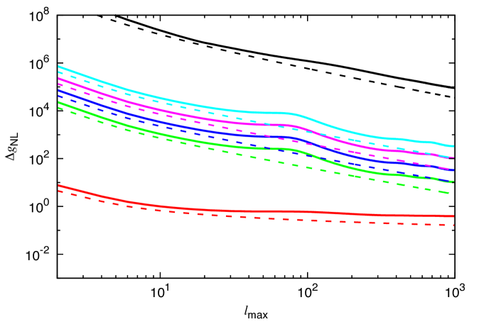
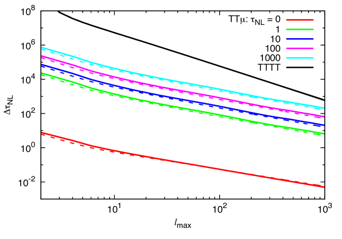
Figure 2: Expected 1$\sigma$ errors on $g_{\textrm{NL}}$ (top panel) and $\tau_{\textrm{NL}}$ (bottom panel) estimated from $TT\mu$ (colored lines) and $TTTT$ (black lines) in the cosmic-variance dominated case (i.e., $N_{\ell}^{\mu\mu}=0$). Solid and dashed lines are the full radiation transfer case (Eqs. (3.32) and (3.38) for $TT\mu$) and the SW case (Eqs. (3.33) and (3.41) for $TT\mu$), respectively. In the $TT\mu$ cases, we consider several nonzero $\tau_{\textrm{NL}}$’s with $f_{\textrm{NL}}=0$. For $\tau_{\textrm{NL}}=0$, $\Delta g_{\textrm{NL}}$ and $\Delta\tau_{\textrm{NL}}$ obtained from $TT\mu$ scale like $1/\ln(\ell_{\rm max}/2)$ and $1/\ell_{\rm max}$, respectively (see Eqs. (4.4) and (4.7)). It is apparent that, if $\tau_{\textrm{NL}}\leq 1000$, for $\ell_{\rm max}\leq 1000$, $TT\mu$ always outperforms $TTTT$, because $C_{\ell}^{\mu\mu,\rm G}+C_{\ell}^{\mu\mu,\tau_{\textrm{NL}}}\ll C_{\ell}^{TT}$. At larger $\ell_{\rm max}$, $TT\mu$ remains clearly superior to $TTTT$ for $g_{\textrm{NL}}$ measurements. For $\tau_{\textrm{NL}}$ estimation the comparison is instead dependent on the fiducial value of $\tau_{\textrm{NL}}$; see main text for further discussion.

The expected $1\sigma$ errors on $g_{\textrm{NL}}$ and $\tau_{\textrm{NL}}$, given by $\Delta g_{\textrm{NL}},\Delta\tau_{\textrm{NL}}=1/\sqrt{F^{TT\mu}}$, in the cosmic variance dominated regime are shown in Fig. 2. For a futuristic, cosmic variance dominated experiment up to $\ell\sim 1000$ (in $\mu$), we can see that spectral distortion based estimators can produce extremely tight error bars, $\Delta g_{\textrm{NL}}\simeq 0.4$ and $\Delta\tau_{\textrm{NL}}\simeq 5\times 10^{-3}$, for fiducial values $f_{\textrm{NL}}=0$, and $\tau_{\textrm{NL}}=0$. This, as originally pointed out in [27], is due to the fact that $\mu$ spectral distortions provide (integrated) information up to very high wavenumbers. However, if we have $\tau_{\textrm{NL}}\neq 0$, the sensitivity is reduced due to the increase of $C_{\ell}^{\mu\mu}$, as described in Fig. 2. This in particular implies that $\tau_{\textrm{NL}}=5\times 10^{-3}$ is not the smallest detectable $\tau_{\textrm{NL}}$, since the error bar computed for this central value satisfies $\Delta\tau_{\textrm{NL}}|_{\tau_{\textrm{NL}}=5\times 10^{-3}}>5\times 10^{-3}$. An inspection of the bottom panel of Fig. 2 and a fact that $\Delta\tau_{\textrm{NL}}$ scales like $\sqrt{\tau_{\textrm{NL}}}$ for $\tau_{\textrm{NL}}\gtrsim 1$ and $\ell\lesssim 1000$ (due to $C_{\ell}^{\mu\mu,\tau_{\textrm{NL}}}\sim 5\times 10^{-23}\tau_{\textrm{NL}}\ell^{-2}\gg C_{\ell}^{\mu\mu,\rm G}$) shows that the smallest value of the parameter for which $\Delta\tau_{\textrm{NL}}|_{\tau_{\textrm{NL}}={\bar{\tau}}_{\rm NL}}<\bar{\tau}_{\rm NL}$ (at $\ell_{\rm max}=1000$) corresponds to $\bar{\tau}_{\rm NL}\sim 40$.

To understand the $\ell_{\rm max}$ dependence of $\Delta g_{\textrm{NL}}$ and $\Delta\tau_{\textrm{NL}}$, we can estimate Eq. (4.1) analytically, using the flat-sky approximation [52, 53]

$$F^{TT\mu}\simeq\frac{1}{\pi(2\pi)^{2}}\left[\prod_{n=1}^{3}\int d^{2}\boldsymbol{\ell}_{n}\right]\delta^{(2)}\left(\boldsymbol{\ell}_{1}+\boldsymbol{\ell}_{2}+\boldsymbol{\ell}_{3}\right)\frac{\left(\hat{b}_{\ell_{1}\ell_{2}\ell_{3}}^{TT\mu}\right)^{2}}{2C_{\ell_{1}}^{TT}C_{\ell_{2}}^{TT}C_{\ell_{3}}^{\mu\mu}}~{}.$$ (4.2)

This should be accurate for large $\ell$. For simplicity, we work here with the SW formulae (3.33) and (3.41) and assume $\tau_{\rm NL}=0$, i.e., $C_{\ell}^{\mu\mu}=C_{\ell}^{\mu\mu,\rm G}=\rm const$. For the $g_{\textrm{NL}}$ case, there is no $\ell_{3}$ dependence except in the delta function, thus, the integral part is reduced to

$$\int_{2}^{\ell_{\rm max}}\ell_{1}d\ell_{1}\,C_{\ell_{1},\rm SW}^{TT}\int_{2}^{\ell_{\rm max}}\ell_{2}d\ell_{2}\,C_{\ell_{2},\rm SW}^{TT}~{}.$$ (4.3)

After computing this, we finally obtain

$$\Delta g_{\textrm{NL}}|_{\tau_{\textrm{NL}}=0}\simeq\left(\frac{C_{\ell}^{\mu\mu,\rm G}}{10^{-30}}\right)^{1/2}\left[\ln\left(\frac{\ell_{\rm max}}{2}\right)\right]^{-1}~{}.$$ (4.4)

For the $\tau_{\textrm{NL}}$ case, the Fisher matrix is proportional to

$$\left[\prod_{n=1}^{3}\int d^{2}\boldsymbol{\ell}_{n}\right]\delta^{(2)}\left(\boldsymbol{\ell}_{1}+\boldsymbol{\ell}_{2}+\boldsymbol{\ell}_{3}\right)\left(\frac{C_{\ell_{1},\rm SW}^{TT}}{C_{\ell_{2},\rm SW}^{TT}}+2+\frac{C_{\ell_{2},\rm SW}^{TT}}{C_{\ell_{1},\rm SW}^{TT}}\right)\left(C_{\ell_{3},\rm SW}^{TT}\right)^{2}~{}.$$ (4.5)

The signals satisfying $\ell_{3}\ll\ell_{1},\ell_{2}$ contribute dominantly to the integrals and hence we can evaluate this as

$$16\pi^{2}\int_{2}^{\ell_{\rm max}}\ell_{1}d\ell_{1}\int_{2}^{\ell_{\rm max}}\ell_{3}d\ell_{3}\left(C_{\ell_{3},\rm SW}^{TT}\right)^{2}~{}.$$ (4.6)

For large $\ell_{\rm max}$, this is proportional to $\ell_{\rm max}^{2}$ and we finally have

$$\Delta\tau_{\textrm{NL}}|_{\tau_{\textrm{NL}}=0}\simeq\left(\frac{C_{\ell}^{\mu\mu,\rm G}}{10^{-30}}\right)^{1/2}\frac{5.5}{\ell_{\rm max}}~{}.$$ (4.7)

For $\ell_{\rm max}\gtrsim 10$, the analytic expressions (4.4) and (4.7) are in excellent agreement with the numerical results (corresponding to the red dashed lines in Fig. 2). On the other hand, for $\tau_{\textrm{NL}}\neq 0$, $\Delta g_{\textrm{NL}}$ deviates drastically from $\propto 1/\ln(\ell_{\rm max}/2)$, because of non-negligible contributions of $C_{\ell}^{\mu\mu,\tau_{\textrm{NL}}}$ to the denominator of the Fisher matrix.

For comparison, in Fig. 2, we also plot our expected uncertainties estimated in a noiseless, cosmic-variance dominated measurement of the CMB temperature trispectrum ($TTTT$), which agree with results in previous literature [54, 55, 56, 57, 58]. This level of sensitivity is essentially already achieved using current Planck data [6, 5]. As shown in this figure, since the cosmic variance uncertainty for $\mu$-distortions is smaller than that for temperature anisotropies (i.e., $C_{\ell}^{\mu\mu,\rm G}+C_{\ell}^{\mu\mu,\tau_{\textrm{NL}}}\ll C_{\ell}^{TT}$), $TT\mu$ allows to achieve better sensitivity to both $g_{\textrm{NL}}$ and $\tau_{\textrm{NL}}$ than $TTTT$ does, for $\ell_{\rm max}\leq 1000$. However, given the difference in scaling with $\ell_{\rm max}$ of the two quantities – i.e. $\Delta\tau_{\textrm{NL}}^{TT\mu}\propto\ell_{\rm max}^{-1}$ (4.7) vs. $\Delta\tau_{\textrm{NL}}^{TTTT}\propto\ell_{\rm max}^{-2}$ [54] – $TTTT$ might become better than $TT\mu$ at measuring $\tau_{\textrm{NL}}$ for higher $\ell_{\rm max}$, and large values of $\tau_{\textrm{NL}}$.

4.2 Effects of experimental uncertainties

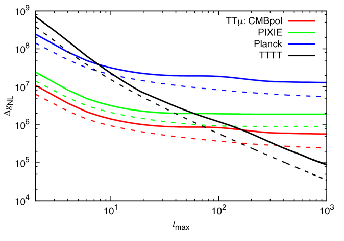
Figure 3: Expected $1\sigma$ errors on $g_{\textrm{NL}}$ computed from $TT\mu$ (colored lines) for noise-levels representative of Planck, PIXIE and CMBpol. For comparison, we also plot the errors computed from $TTTT$ (black lines) for a noiseless CMB survey, which are almost the same as the errors obtained in the Planck temperature data analysis [6, 5]. Solid and dashed lines correspond to the results including full CMB transfer function (Eqs. (3.32) and (3.38) for $TT\mu$) and those in the SW limit (Eqs. (3.33) and (3.41) for $TT\mu$), respectively. We here assume $f_{\textrm{NL}}=\tau_{\textrm{NL}}=0$. For $\ell_{\rm max}\lesssim\ell_{\mu}$, the scalings agree with expectations from Eqs. (4.1) and (4.4): $\Delta g_{\textrm{NL}}\simeq(N_{\mu}/10^{-30})^{1/2}[\ln(\ell_{\rm max}/2)]^{-1}$. At larger $\ell_{\rm max}$, when $N_{\mu}$ starts dominating, the $TT\mu$ sensitivity falls below $TTTT$.

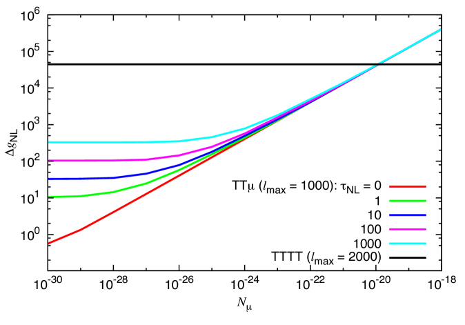
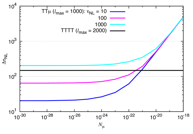
Figure 4: Expected 1$\sigma$ errors on $g_{\textrm{NL}}$ (top panel) and $\tau_{\textrm{NL}}$ (bottom panel) estimated from $TT\mu$ (colored lines) at $\ell_{\rm max}=1000$, as a function of the magnitude of instrumental noise $N_{\mu}$, keeping $\ell_{\mu}=1000$ angular resolution fixed. Black lines show the expected errors, at $\ell_{\rm max}=2000$, obtained from $TTTT$ in a noiseless CMB measurement, very close to the error bars obtained from the Planck temperature data [6, 5]. In the $TT\mu$ cases, we consider several nonzero $\tau_{\textrm{NL}}$’s with $f_{\textrm{NL}}=0$. The $TT\mu$ bispectrum used in this estimation is computed from Eqs. (3.32) and (3.38), including the full CMB transfer function dependence.

Besides the ideal, cosmic-variance dominated case, we consider also several different noise levels, corresponding to experiments like Planck [59], PIXIE [60] and CMBpol [61]. For $\mu$-$\mu$ noise spectra, we assume $N_{\ell}^{\mu\mu}=N_{\mu}\textrm{exp}\left(\ell^{2}/\ell_{\mu}^{2}\right)$, with $(N_{\mu},\ell_{\mu})=(10^{-15},861)$ (Planck), $(10^{-17},84)$ (PIXIE) and $(2\times 10^{-18},1000)$ (CMBpol) [28, 32]. As it is typical for this type of analysis, we see that current and forthcoming surveys, such as Planck and PIXIE, are expected to produce error bars on relevant NG parameters which are much worse than what is achievable with the current Planck measurements or cosmic-variance dominated CMB measurements (compare colored lines with black lines in Fig. 3). If we focus on $g_{\textrm{NL}}$, and consider the fiducial case $\tau_{\textrm{NL}}=0$ (resulting in $C_{\ell}^{\mu\mu}=C_{\ell}^{\mu\mu,\rm G}+N_{\ell}^{\mu\mu}$), we find that Planck can achieve a level of sensitivity $\Delta g_{\textrm{NL}}\simeq 10^{7}$, while PIXIE and CMBpol are expected to reach $\Delta g_{\textrm{NL}}\simeq 2\times 10^{6}$ and $\Delta g_{\textrm{NL}}\simeq 6\times 10^{5}$, respectively, as described in Fig. 3.

It is interesting to estimate the noise level in $\mu$-distortion measurements, required for $TT\mu$ to achieve better sensitivity than $TTTT$. To this purpose, we compute $\Delta g_{\textrm{NL}}$ and $\Delta\tau_{\textrm{NL}}$ at $\ell_{\rm max}=1000$, gradually decreasing the magnitude of instrumental noise, $N_{\mu}$, from $10^{-18}$ to $10^{-30}$. For the angular resolution, we consider $\ell_{\mu}=1000$, comparable to the value in CMBpol [61]. Figure 4 describes our numerical results. For large $N_{\mu}$, $C_{\ell}^{\mu\mu}$, at the denominator of (4.1), is dominated by instrumental noise. The error bars thus scale like $\sqrt{N_{\mu}}$. However, as $N_{\mu}$ decreases, $N_{\ell}^{\mu\mu}$ becomes subdominant compared with $C_{\ell}^{\mu\mu,\tau_{\textrm{NL}}}$ or $C_{\ell}^{\mu\mu,\rm G}$, and the error bars finally plateau for $N_{\mu}\lesssim C_{\ell}^{\mu\mu,\rm G}\sim 10^{-30}$. This behavior is displayed in Fig. 4, for several fiducial values of $\tau_{\textrm{NL}}$. We find from the top panel of Fig. 4 that, if we want $TT\mu$ to outperform $TTTT$ at measuring $g_{\textrm{NL}}$, $N_{\mu}\lesssim 10^{-20}$ is required, independently of $\tau_{\textrm{NL}}$. In contrast, for the $\tau_{\textrm{NL}}$ case, the final result depends strongly on the actual value of $\tau_{\textrm{NL}}$. We have already seen in the previous subsection that a detectable $\tau_{\textrm{NL}}$ should obey $\Delta\tau_{\textrm{NL}}<\tau_{\textrm{NL}}$, making $\tau_{\textrm{NL}}\sim 40$ the smallest detectable value, for $N_{\mu}=0$. For this reason $TT\mu$ is not useful for measuring small values of $\tau_{\textrm{NL}}$. Nonetheless, as seen in the bottom panel of Fig. 4, $\tau_{\textrm{NL}}\sim 100$ is detectable using $TT\mu$, when $N_{\mu}\lesssim 10^{-23}$, while being unmeasurable with $TTTT$. If we further increase $\tau_{\textrm{NL}}$ to reach $\tau_{\textrm{NL}}\sim 1000$, then $TTTT$ outperforms $TT\mu$. Of course, the most powerful way to measure $\tau_{\textrm{NL}}$ using spectral distortions is via $\mu\mu$ correlations [27], and that approach can potentially vastly outperform the temperature trispectrum. If we consider $\tau_{\textrm{NL}}$, $TT\mu$ can be essentially used for a cross-check of tighter $\mu\mu$ results.

5 Conclusions

In this paper, we studied the $TT\mu$ three-point function, arising from correlations between CMB temperature anisotropies and chemical potential ($\mu$) distortions in presence of local primordial NG. We showed, first with a more intuitive argument, followed by a full calculation, that both $\tau_{\textrm{NL}}$ and $g_{\textrm{NL}}$-type primordial trispectrum signatures source the $TT\mu$ bispectrum. Measurements of $TT\mu$ would thus allow to constrain also the $g_{\textrm{NL}}$ parameter, contrary to what happens with the $\mu\mu$ two-point auto-correlation, which is sensitive only to the $\tau_{\textrm{NL}}$ signal [27]. Our Fisher matrix-based forecast, in line with previous $T\mu$ and $\mu\mu$ analyses [27, 28, 29, 30, 31, 32, 33, 34, 35], shows that an ideal, cosmic-variance dominated experiment could in principle determine $g_{\textrm{NL}}$ and $\tau_{\textrm{NL}}$ from $TT\mu$ with an impressive level of accuracy, allowing to detect $g_{\textrm{NL}}\sim 0.4$ and $\tau_{\textrm{NL}}\sim 40$. While this is obviously a futuristic scenario, it does reflect the fact that correlations between CMB anisotropies and spectral distortions, including two and three-point functions, contain a large amount of information (since they can probe a vast range of otherwise unaccessible scales), and have the potential to significantly improve on current primordial NG experimental bounds.

The exact shape of the $TT\mu$ bispectrum should depend on the primordial inflationary scenario under exam. For example, in an inflationary model where a vector field acts as a strong NG source (e.g., [62, 63, 64]), a direction dependence of the vector field in the curvature trispectrum may give nontrivial effects in $TT\mu$, as well as it does for $TTT$ [62, 65, 66], $TTTT$ [56] and $T\mu$ [35]. Moreover, $TT\mu$ could also arise from different generation mechanisms. Heating sources, such as magnetic fields stretched on cosmological scales, can generate $T$ and $\mu$ fields which differs from the standard adiabatic mode considered in this paper (e.g., [31, 30, 32]). Also in this case one expects a $TT\mu$ signature with a specific shape. $TT\mu$ could be interesting also to check alternative models to Inflation. For example, it was argued that ekpyrosis produces a local trispectrum with $g_{\textrm{NL}}\leq-1700$ [67] or $-1000\leq g_{\textrm{NL}}\leq-100$ [68], a value which is well below the sensitivity of CMB temperature trispectrum measurements, but that is in principle accessible with $TT\mu$ in the future, according to our results. As a starting point, this paper analyzed the most standard case, namely, $TT\mu$ sourced by the adiabatic mode due to the standard $g_{\textrm{NL}}$ and $\tau_{\textrm{NL}}$-type trispectra. Other possibilities, mentioned above, are interesting to investigate and will be accounted for in future works.

References

• [1] D. S. Salopek and J. R. Bond, Nonlinear evolution of long wavelength metric fluctuations in inflationary models, Phys. Rev. D42 (1990) 3936–3962.
• [2] A. Gangui, F. Lucchin, S. Matarrese and S. Mollerach, The Three point correlation function of the cosmic microwave background in inflationary models, Astrophys. J. 430 (1994) 447–457, [astro-ph/9312033].
• [3] K. M. Smith, L. Senatore and M. Zaldarriaga, Optimal analysis of the CMB trispectrum, 1502.00635.
• [4] Planck collaboration, P. Ade et al., Planck 2013 Results. XXIV. Constraints on primordial non-Gaussianity, Astron.Astrophys. 571 (2014) A24, [1303.5084].
• [5] C. Feng, A. Cooray, J. Smidt, J. O’Bryan, B. Keating and D. Regan, Planck Trispectrum Constraints on Primordial Non-Gaussianity at Cubic Order, Phys. Rev. D92 (2015) 043509, [1502.00585].
• [6] Planck collaboration, P. A. R. Ade et al., Planck 2015 results. XVII. Constraints on primordial non-Gaussianity, 1502.01592.
• [7] T. Suyama and M. Yamaguchi, Non-Gaussianity in the modulated reheating scenario, Phys. Rev. D77 (2008) 023505, [0709.2545].
• [8] M. Sasaki, J. Valiviita and D. Wands, Non-Gaussianity of the primordial perturbation in the curvaton model, Phys. Rev. D74 (2006) 103003, [astro-ph/0607627].
• [9] C. T. Byrnes, M. Sasaki and D. Wands, The primordial trispectrum from inflation, Phys. Rev. D74 (2006) 123519, [astro-ph/0611075].
• [10] C. T. Byrnes and K.-Y. Choi, Review of local non-Gaussianity from multi-field inflation, Adv. Astron. 2010 (2010) 724525, [1002.3110].
• [11] K. Ichikawa, T. Suyama, T. Takahashi and M. Yamaguchi, Primordial Curvature Fluctuation and Its Non-Gaussianity in Models with Modulated Reheating, Phys. Rev. D78 (2008) 063545, [0807.3988].
• [12] L. Senatore and M. Zaldarriaga, A Naturally Large Four-Point Function in Single Field Inflation, JCAP 1101 (2011) 003, [1004.1201].
• [13] D. Baumann and D. Green, Signatures of Supersymmetry from the Early Universe, Phys. Rev. D85 (2012) 103520, [1109.0292].
• [14] N. Bartolo, M. Fasiello, S. Matarrese and A. Riotto, Large non-Gaussianities in the Effective Field Theory Approach to Single-Field Inflation: the Trispectrum, JCAP 1009 (2010) 035, [1006.5411].
• [15] EUCLID collaboration, R. Laureijs et al., Euclid Definition Study Report, 1110.3193.
• [16] T. Giannantonio, C. Porciani, J. Carron, A. Amara and A. Pillepich, Constraining primordial non-Gaussianity with future galaxy surveys, MNRAS 422 (June, 2012) 2854–2877, [1109.0958].
• [17] A. R. Cooray and W. Hu, Imprint of reionization on the cosmic microwave background bispectrum, Astrophys. J. 534 (2000) 533–550, [astro-ph/9910397].
• [18] A. Cooray, Large-scale non-Gaussianities in the 21 cm background anisotropies from the era of reionization, Mon. Not. Roy. Astron. Soc. 363 (2005) 1049, [astro-ph/0411430].
• [19] A. Cooray, C. Li and A. Melchiorri, The trispectrum of 21-cm background anisotropies as a probe of primordial non-Gaussianity, Phys. Rev. D77 (2008) 103506, [0801.3463].
• [20] A. Pillepich, C. Porciani and S. Matarrese, The bispectrum of redshifted 21-cm fluctuations from the dark ages, Astrophys. J. 662 (2007) 1–14, [astro-ph/0611126].
• [21] J. B. Muñoz, Y. Ali-Haïmoud and M. Kamionkowski, Primordial non-gaussianity from the bispectrum of 21-cm fluctuations in the dark ages, Phys. Rev. D92 (2015) 083508, [1506.04152].
• [22] H. Shimabukuro, S. Yoshiura, K. Takahashi, S. Yokoyama and K. Ichiki, 21cm-line bispectrum as method to probe Cosmic Dawn and Epoch of Reionization, 1507.01335.
• [23] T. Giannantonio, C. Porciani, J. Carron, A. Amara and A. Pillepich, Constraining primordial non-Gaussianity with future galaxy surveys, Mon. Not. Roy. Astron. Soc. 422 (2012) 2854–2877, [1109.0958].
• [24] R. Maartens, G.-B. Zhao, D. Bacon, K. Koyama and A. Raccanelli, Relativistic corrections and non-Gaussianity in radio continuum surveys, JCAP 1302 (2013) 044, [1206.0732].
• [25] J. Byun and R. Bean, Non-Gaussian Shape Discrimination with Spectroscopic Galaxy Surveys, JCAP 1503 (2015) 019, [1409.5440].
• [26] A. Raccanelli, M. Shiraishi, N. Bartolo, D. Bertacca, M. Liguori, S. Matarrese et al., Future Constraints on Angle-Dependent Non-Gaussianity from Large Radio Surveys, 1507.05903.
• [27] E. Pajer and M. Zaldarriaga, A New Window on Primordial non-Gaussianity, Phys.Rev.Lett. 109 (2012) 021302, [1201.5375].
• [28] J. Ganc and E. Komatsu, Scale-dependent bias of galaxies and mu-type distortion of the cosmic microwave background spectrum from single-field inflation with a modified initial state, Phys.Rev. D86 (2012) 023518, [1204.4241].
• [29] M. Biagetti, H. Perrier, A. Riotto and V. Desjacques, Testing the running of non-Gaussianity through the CMB $\mu$-distortion and the halo bias, Phys.Rev. D87 (2013) 063521, [1301.2771].
• [30] K. Miyamoto, T. Sekiguchi, H. Tashiro and S. Yokoyama, CMB distortion anisotropies due to the decay of primordial magnetic fields, Phys.Rev. D89 (2014) 063508, [1310.3886].
• [31] K. E. Kunze and E. Komatsu, Constraining primordial magnetic fields with distortions of the black-body spectrum of the cosmic microwave background: pre- and post-decoupling contributions, JCAP 1401 (2014) 009, [1309.7994].
• [32] J. Ganc and M. S. Sloth, Probing correlations of early magnetic fields using mu-distortion, JCAP 1408 (2014) 018, [1404.5957].
• [33] A. Ota, T. Sekiguchi, Y. Tada and S. Yokoyama, Anisotropic CMB distortions from non-Gaussian isocurvature perturbations, JCAP 1503 (2015) 013, [1412.4517].
• [34] R. Emami, E. Dimastrogiovanni, J. Chluba and M. Kamionkowski, Probing the scale dependence of non-Gaussianity with spectral distortions of the cosmic microwave background, Phys. Rev. D91 (2015) 123531, [1504.00675].
• [35] M. Shiraishi, M. Liguori, N. Bartolo and S. Matarrese, Measuring primordial anisotropic correlators with CMB spectral distortions, Phys. Rev. D92 (2015) 083502, [1506.06670].
• [36] R. Khatri and R. Sunyaev, Constraints on $\mu$-distortion fluctuations and primordial non-Gaussianity from Planck data, JCAP 1509 (2015) 026, [1507.05615].
• [37] J. Silk, Cosmic Black-Body Radiation and Galaxy Formation, ApJ 151 (Feb., 1968) 459.
• [38] P. J. E. Peebles and J. T. Yu, Primeval Adiabatic Perturbation in an Expanding Universe, ApJ 162 (Dec., 1970) 815.
• [39] N. Kaiser, Small-angle anisotropy of the microwave background radiation in the adiabatic theory, MNRAS 202 (Mar., 1983) 1169–1180.
• [40] S. Weinberg, Cosmology. Oxford University Press, 2008.
• [41] R. A. Sunyaev and Ya. B. Zeldovich, The Interaction of matter and radiation in the hot model of the universe, Astrophys. Space Sci. 7 (1970) 20–30.
• [42] A. F. Illarionov and R. A. Siuniaev, Comptonization, characteristic radiation spectra, and thermal balance of low-density plasma, Soviet Ast. 18 (Feb., 1975) 413–419.
• [43] L. Danese and G. de Zotti, Double Compton process and the spectrum of the microwave background, A&A 107 (Mar., 1982) 39–42.
• [44] C. Burigana, L. Danese and G. de Zotti, Formation and evolution of early distortions of the microwave background spectrum - A numerical study, A&A 246 (June, 1991) 49–58.
• [45] W. Hu, D. Scott and J. Silk, Power spectrum constraints from spectral distortions in the cosmic microwave background, Astrophys.J. 430 (1994) L5–L8, [astro-ph/9402045].
• [46] J. Chluba and R. Sunyaev, The evolution of CMB spectral distortions in the early Universe, Mon.Not.Roy.Astron.Soc. 419 (2012) 1294–1314, [1109.6552].
• [47] R. Khatri, R. A. Sunyaev and J. Chluba, Does Bose-Einstein condensation of CMB photons cancel $\mu$ distortions created by dissipation of sound waves in the early Universe?, Astron.Astrophys. 540 (2012) A124, [1110.0475].
• [48] J. Chluba, R. Khatri and R. A. Sunyaev, CMB at 2x2 order: The dissipation of primordial acoustic waves and the observable part of the associated energy release, Mon.Not.Roy.Astron.Soc. 425 (2012) 1129–1169, [1202.0057].
• [49] R. Khatri and R. A. Sunyaev, Creation of the CMB spectrum: precise analytic solutions for the blackbody photosphere, JCAP 1206 (2012) 038, [1203.2601].
• [50] R. Khatri and R. A. Sunyaev, Beyond y and $\mu$: the shape of the CMB spectral distortions in the intermediate epoch, $1.5\times 10^{4}<z<2\times 10^{5}$, JCAP 1209 (2012) 016, [1207.6654].
• [51] E. Komatsu and D. N. Spergel, Acoustic signatures in the primary microwave background bispectrum, Phys.Rev. D63 (2001) 063002, [astro-ph/0005036].
• [52] W. Hu, Weak lensing of the CMB: A harmonic approach, Phys. Rev. D62 (2000) 043007, [astro-ph/0001303].
• [53] D. Babich and M. Zaldarriaga, Primordial bispectrum information from CMB polarization, Phys. Rev. D70 (2004) 083005, [astro-ph/0408455].
• [54] N. Kogo and E. Komatsu, Angular trispectrum of cmb temperature anisotropy from primordial non-gaussianity with the full radiation transfer function, Phys. Rev. D73 (2006) 083007, [astro-ph/0602099].
• [55] R. Pearson, A. Lewis and D. Regan, CMB lensing and primordial squeezed non-Gaussianity, JCAP 1203 (2012) 011, [1201.1010].
• [56] M. Shiraishi, E. Komatsu and M. Peloso, Signatures of anisotropic sources in the trispectrum of the cosmic microwave background, JCAP 1404 (2014) 027, [1312.5221].
• [57] D. M. Regan, E. P. S. Shellard and J. R. Fergusson, General CMB and Primordial Trispectrum Estimation, Phys. Rev. D82 (2010) 023520, [1004.2915].
• [58] T. Sekiguchi and N. Sugiyama, Optimal constraint on $g_{NL}$ from CMB, JCAP 1309 (2013) 002, [1303.4626].
• [59] Planck collaboration, J. Tauber et al., The Scientific programme of Planck, astro-ph/0604069.
• [60] A. Kogut, D. Fixsen, D. Chuss, J. Dotson, E. Dwek et al., The Primordial Inflation Explorer (PIXIE): A Nulling Polarimeter for Cosmic Microwave Background Observations, JCAP 1107 (2011) 025, [1105.2044].
• [61] CMBPol Study Team collaboration, D. Baumann et al., CMBPol Mission Concept Study: Probing Inflation with CMB Polarization, AIP Conf.Proc. 1141 (2009) 10–120, [0811.3919].
• [62] N. Bartolo, E. Dimastrogiovanni, M. Liguori, S. Matarrese and A. Riotto, An Estimator for statistical anisotropy from the CMB bispectrum, JCAP 1201 (2012) 029, [1107.4304].
• [63] N. Bartolo, S. Matarrese, M. Peloso and A. Ricciardone, Anisotropic power spectrum and bispectrum in the $f(\phi)F^{2}$ mechanism, Phys.Rev. D87 (2013) 023504, [1210.3257].
• [64] N. Bartolo, S. Matarrese, M. Peloso and M. Shiraishi, Parity-violating CMB correlators with non-decaying statistical anisotropy, JCAP 1507 (2015) 039, [1505.02193].
• [65] M. Shiraishi and S. Yokoyama, Violation of the Rotational Invariance in the CMB Bispectrum, Prog.Theor.Phys. 126 (2011) 923–935, [1107.0682].
• [66] M. Shiraishi, E. Komatsu, M. Peloso and N. Barnaby, Signatures of anisotropic sources in the squeezed-limit bispectrum of the cosmic microwave background, JCAP 1305 (2013) 002, [1302.3056].
• [67] J.-L. Lehners and P. J. Steinhardt, Planck 2013 results support the cyclic universe, Phys. Rev. D87 (2013) 123533, [1304.3122].
• [68] A. Fertig and J.-L. Lehners, The Non-Minimal Ekpyrotic Trispectrum, 1510.03439.