Kinetically Modified Non-Minimal Higgs Inflation in Supergravity

Abstract

Abstract: We consider models of chaotic inflation driven by the real parts of a conjugate pair of Higgs superfields involved in the spontaneous breaking of a grand unification symmetry at a scale assuming its supersymmetric value. We combine a superpotential, which is uniquely determined by applying a continuous $R$ symmetry, with a class of logarithmic or semi-logarithmic Kähler potentials which exhibit a prominent shift-symmetry with a tiny violation, whose strengths are quantified by $c_{-}$ and $c_{+}$ respectively. The inflationary observables provide an excellent match to the recent Bicep2/Keck Array and Planck results setting $3.5\cdot 10^{-3}\lesssim r_{\pm}=c_{+}/c_{-}\lesssim 1/N$ where $N=3$ or $2$ is the prefactor of the logarithm. Inflation can be attained for subplanckian inflaton values with the corresponding effective theories retaining the perturbative unitarity up to the Planck scale.

PACs numbers: 98.80.Cq, 04.50.Kd, 12.60.Jv, 04.65.+e Published in Phys. Rev. D 92, no. 12, 121305(R) (2015)

I Introduction

Soon after inflation’s guth introduction as a solution to a number of longstanding cosmological puzzles – such as the horizon and flatness problems – many efforts have been made so as to connect it with a Grand Unified Theory (GUT) phase transition in the early universe – see e.g. Refs. old ; fhi ; jones2 ; nmH ; lazarides ; fhi1 ; fhi2 ; fhi3 ; okada . According to this economical and highly appealing set-up, the scalar field which drives inflation (called inflaton) plays, at the end of its inflationary evolution, the role of a Higgs field old ; jones2 ; nmH ; okada ; lazarides or destabilizes others fields, which act as Higgs fields fhi ; fhi1 ; fhi2 ; fhi3 ; fhi4 . As a consequence, a GUT gauge group $G_{\rm GUT}$ can be spontaneously broken after the end of inflation. The first mechanism above can be also applied in the context of the Standard Model (SM) sm or the next-to-Minimal Supersymmetric SM (MSSM) linde1 ; shiftHI and leads to the spontaneous breaking of the electroweak gauge group ${G_{\rm SM}}=SU(3)_{\rm C}\times SU(2)_{\rm L}\times U(1)_{Y}$ by the Higgs/inflaton field(s).

We here focus on the earlier version of this idea – i.e. the GUT-scale Higgs inflation – concentrating on its supersymmetric (SUSY) realization fhi ; jones2 ; nmH ; lazarides ; fhi1 ; fhi2 ; fhi3 ; fhi4 ; okada , where the notorious GUT hierarchy problem is elegantly addressed. The starting point of our approach is the simplest superpotential

$$W=\lambda S\left(\bar{\Phi}\Phi-M^{2}/4\right)$$ (1)

which leads to the spontaneous breaking of $G_{\rm GUT}$ and is uniquely determined, at renormalizable level, by a convenient fhi continuous $R$ symmetry. Here, $\lambda$ and $M$ are two constants which can both be taken positive by field redefinitions; $S$ is a left-handed superfield, singlet under $G_{\rm GUT}$; $\bar{\Phi}$ and $\Phi$ is a pair of left-handed superfields belonging to non-trivial conjugate representations of $G_{\rm GUT}$, and reducing its rank by their vacuum expectation values (v.e.vs) – see e.g. Refs. fhi1 ; fhi2 . Just for definiteness we restrict ourselves to $G_{\rm GUT}=G_{\rm SM}\times U(1)_{B-L}$ fhi1 ; okada , gauge group which consists the simplest GUT beyond the MSSM – where $B$ and $L$ denote the baryon and lepton number. With the specific choice of $G_{\rm GUT}$ $\Phi$ and $\bar{\Phi}$ carry $B-L$ charges $1$ and $-1$ respectively.

Moreover, $W$ combined with a judiciously selected Kähler potential, $K$, gives rise to two types of inflation, in the context of Supergravity (SUGRA). In particular, we can obtain F-term hybrid inflation (FHI) driven by $S$ with $\bar{\Phi}$ and $\Phi$ being confined to zero or non-minimal Higgs inflation (nMHI), interchanging the roles of $S$ and $\bar{\Phi}-\Phi$. A canonical fhi1 or quasi-canonical fhi3 ; fhi2 $K$ is convenient for implementing FHI, whereas a logarithmic $K$ including an holomorphic function $c_{\cal R}\Phi\bar{\Phi}$ with large $c_{\cal R}>0$ nmH or tiny $c_{\cal R}<0$ okada is dictated for nMHI. Although FHI can become compatible with data plcp at the cost of a mild tuning of one fhi1 ; fhi3 (or more fhi2 ) parameters beyond $\lambda$ and $M$, it exhibits a serious drawback which can be eluded, by construction, in nMHI. Since $G_{\rm GUT}$ is broken only at the SUSY vacuum, after the end of FHI, topological defects are formed, if they are predicted by the $G_{\rm GUT}$ breaking. This does not occur within nMHI since $G_{\rm GUT}$ is already spontaneously broken during it, through the non-zero $\bar{\Phi}$ and $\Phi$ values. Utilizing large enough $c_{\cal R}$’s nmH or adjusting three parameters ($\lambda$, $c_{\cal R}$ and $M$) okada , acceptable values for the (scalar) spectral index, $n_{\rm s}$, can be achieved with low enough nmH or higher okada tensor-to-scalar ratio, $r$. In the former case, though, the largeness of $c_{\cal R}$ violates the perturbative unitarity cutoff ; riotto whereas in the latter case, transplanckian values of the inflaton jeopardize the validity of the inflationary predictions.

In this letter, we show that the shortcomings above can be elegantly overcome, if we realize the recently proposed nMkin idea of kinetically modified non-minimal inflation with a $G_{\rm GUT}$ non-singlet inflaton. The crucial difference of this setting compared to the nMHI with large $c_{\cal R}$ nmH is that the slope of the inflationary potential and the canonical normalization of the higgs-inflaton do not depend exclusively on one parameter, $c_{\cal R}$, but separately on two parameters, $c_{+}$ and $c_{-}$, whose the ratio $r_{\pm}=c_{+}/c_{-}\ll 1$ determines $n_{\rm s}$ and $r$. In particular, restricting $r_{\pm}$ to natural values, motivated by an enhanced shift symmetry, the inflationary observables can nicely cover the 1-$\sigma$ domain of the present data plcp ; gws ,

$$n_{\rm s}=0.968\pm 0.0045~{}~{}\mbox{and}~{}~{}r=0.048^{+0.035}_{-0.032},$$ (2)

independently of $M$ which may be confined precisely at its value entailed by the gauge unification within MSSM. Contrary to our recent investigation lazarides , where we stick to quadratic terms for $\Phi$ and $\bar{\Phi}$ in the selected $K$’s we here parameterize the relevant terms with an exponent $m$. Moreover, we here, insist to integer prefactors of the logarithms involved in $K$’s, increasing thereby the naturalness of the model. As regards other simple and well-motivated inflationary models roest ; eno5 which share similar inflationary potentials with the one obtained here, let us underline that the use of a gauge non-singlet inflaton with subplanckian values together with the enhanced resulting $r$’s, in accordance with an approximate shift symmetry, consist the main novelties of our approach.

Below we describe a class of Kähler potentials which lead to kinetically modified nMHI, we outline the derivation of the inflationary potential and restrict the free parameters of the models testing them against observations. Finally, we analyze the ultraviolet (UV) behavior of these models and summarize our conclusions.

II Kähler Potentials

The key ingredient of our proposal is the selection of a purely or partially logarithmic $K$ including the real functions

$$F_{\pm}=\left|\Phi\pm\bar{\Phi}^{*}\right|^{2}~{}~{}\mbox{and}~{}~{}F_{S}=|S|^{2}-k_{S}{|S|^{4}},$$ (3)

which respect the symmetries of $W$ – star (^∗) denotes complex conjugation. As we show below, $c_{-}F_{-}$ dominates the canonical normalization of inflaton, $c_{+}F_{+}$ plays the role of the non-minimal inflaton-curvature coupling and $F_{S}$ provides a typical kinetic term for $S$, considering the next-to-minimal term for stability/heaviness reasons linde1 . Obviously, $F_{S}$ is the same as that used in Ref. nMkin , apart from an overall normalization factor, whereas $F_{-}$ and $F_{+}$ correspond to $F_{\rm K}$ and $F_{\cal R}$ respectively. However, $F_{+}$ is a real and not an holomorphic function as $F_{\cal R}$. Actually, it remains invariant under the transformation $\Phi\ \rightarrow\ \Phi+c$ and $\bar{\Phi}\ \rightarrow\ \bar{\Phi}-c^{*}$ (where $c$ is a complex number) whereas $F_{-}$ respects the symmetry $\Phi\ \rightarrow\ \Phi+c$ and $\bar{\Phi}\ \rightarrow\ \bar{\Phi}+c^{*}$ which coincides with the former only for $c=0$. Stability of the selected inflationary direction entails that the latter symmetry is to be the dominant one – see below. The particular importance of the shift symmetry in taming the so-called $\eta$-problem of inflation in SUGRA is first recognized for gauge singlets in Ref. kawasaki and non-singlets in Ref. shiftHI .

In terms of the functions introduced in Eq. (3) we postulate the following form of $K$

$$K_{1} = -3\ln\left(1+c_{+}F_{+}-\frac{1}{3}(1+c_{+}F_{+})^{m}c_{-}F_{-}\right.$$ (4a)

$$\left.-\frac{1}{3}F_{S}+k_{\Phi}F_{-}^{2}+\frac{1}{3}k_{S\Phi}F_{-}{|S|^{2}}\right)\,,~{}~{}~{}~{}~{}$$

where we take for consistency all the possible terms up to fourth order whereas a term of the form $$-k_{S+}F_{+}^{m}|S|^{2}/3 F_{+} m_{\rm P}=2.433\cdot 10^{18}~{}{\mbox{\rm GeV}} K=K_{2}$$ is neglected for simplicity, given that is considered as a violation of the principal symmetry – we use throughout units with the reduced Planck scale being set equal to unity. Identical results can be achieved if we select with

$$K_{2}=-3\ln\left(1+c_{+}F_{+}-\frac{1}{3}F_{S}\right)+\frac{c_{-}F_{-}}{(1+c_{+}F_{+})^{1-m}}\,\cdot$$ (4b)

If we place $$F_{S} K$$ outside the argument of the logarithm, we can obtain two other ’s – not mentioned in Ref. nMkin – which lead to similar results. Namely,

$$K_{3}=-2\ln\left(1+c_{+}F_{+}-\frac{1}{2}(1+c_{+}F_{+})^{m}c_{-}F_{-}\right)+F_{S}\,$$ (4c)

and

$$K_{4}=-2\ln(1+c_{+}F_{+})+F_{S}+(1+c_{+}F_{+})^{m-1}c_{-}F_{-}\,.$$ (4d)

To highlight the robustness of our setting we use only integer prefactors for the logarithms avoiding thereby any relevant tuning – cf. Ref. lazarides ; nIG . Note that for $m=0$ [$m=1$], $F_{-}$ and $F_{+}$ in $K_{1}$ and $K_{3}$ [$K_{2}$ and $K_{4}$] are totally decoupled, i.e. no higher order term is needed. If we allow for a continuous variation of the $\ln$ prefactor, too, we can obtain several variants of kinetically modified nMHI. For $m=0$ this possibility is analyzed in Ref. lazarides .

Given that $M\ll 1$ does not affect the inflationary epoch, the free parameters of our models, for fixed $m$, are $r_{\pm}$ and $\lambda/c_{-}$ and not $c_{-}$, $c_{+}$ and $\lambda$ as naively expected. Indeed, performing the rescalings $\Phi\rightarrow\Phi/\sqrt{c_{-}}$ and $\bar{\Phi}\rightarrow\bar{\Phi}/\sqrt{c_{-}}$, in Eqs. (1) and (4a) – (4d) we see that $W$ and $K$ depends exclusively on $\lambda/c_{-}$ and $r_{\pm}$ respectively. Therefore, our models are equally economical as nMHI with $c_{\cal R}<0$ okada and they have just one more free parameter than nMHI with $c_{\cal R}>0$ nmH – see also Ref. roest . Unlike these models, however, – where the largeness nmH or the smallness okada of $c_{\cal R}$ can not be justified by any symmetry – our models can be characterized as completely natural, in the ’t Hooft sense, since in the limits $r_{\pm}=c_{+}/c_{-}\rightarrow 0$ and $\lambda\rightarrow 0$, they enjoy the following enhanced symmetries:

$$\Phi\rightarrow\ \Phi+c,\>\>\>\bar{\Phi}\rightarrow\ \bar{\Phi}+c^{*}\>\>\>\mbox{and}\>\>\>S\rightarrow\ e^{i\varphi}S,$$ (5)

where $c$ and $\varphi$ is a complex and a real number respectively. The same argument guarantees the smallness of $k_{S+}$ in a possible term $-k_{S+}F_{+}^{m}|S|^{2}/3$ inside the logarithms in Eq. (4a) or Eq. (4b). On the other hand, our models do not exhibit any no-scale-type symmetry like that postulated in Ref. eno5 .

Table 1: Mass-squared spectrum for $K=K_{i}$ and $K=K_{i+2}$ ($i=1,2$) along the path in Eq. (8).

Fields	Eigenstates	Masses Squared
		Symbol	$K=K_{1}$	$K=K_{2}$	$K=K_{i+2}$
2 real scalars	$\widehat{\theta}_{+}$	$\widehat{m}_{\theta+}^{2}$	$4\widehat{H}_{\rm HI}^{2}$	$6\widehat{H}_{\rm HI}^{2}$
	$\widehat{\theta}_{\Phi}$	$\widehat{m}_{\theta_{\Phi}}^{2}$	$M^{2}_{BL}+4\widehat{H}_{\rm HI}^{2}$	$M^{2}_{BL}+6\widehat{H}_{\rm HI}^{2}$
1 complex scalar	$\widehat{s},\widehat{\bar{s}}$	$\widehat{m}_{s}^{2}$	$6\left(2k_{S}f_{\cal R}-1/3\right)\widehat{H}_{\rm HI}^{2}$		$12k_{S}\widehat{H}_{\rm HI}^{2}$
1 gauge boson	$A_{BL}$	$M_{BL}^{2}$	$g^{2}c_{-}\left(f_{\cal R}^{m-1}-Nr_{\pm}/f_{\cal R}\right)\phi^{2}$
$4$ Weyl spinors	$\widehat{\psi}_{\pm}=\frac{1}{\sqrt{2}}(\widehat{\psi}_{\Phi+}\pm\widehat{\psi}_{S})$	$\widehat{m}^{2}_{\psi\pm}$	${24\widehat{H}_{\rm HI}^{2}/c_{-}\phi^{2}f_{\cal R}^{1+m}}$
	$\uplambda_{BL},\widehat{\psi}_{\Phi-}$	$M_{BL}^{2}$	$g^{2}c_{-}\left(f_{\cal R}^{m-1}-Nr_{\pm}/f_{\cal R}\right)\phi^{2}$

III Inflationary Potential

The Einstein frame (EF) action within SUGRA for the complex scalar fields $z^{\alpha}=S,\Phi,\bar{\Phi}$ – denoted by the same superfield symbol – can be written as linde1

$${\sf S}=\int d^{4}x\sqrt{-\widehat{\mathfrak{g}}}\left(-\frac{1}{2}\widehat{\mathcal{R}}+K_{{\alpha}{\bar{\beta}}}\widehat{g}^{\mu\nu}D_{\mu}z^{\alpha}D_{\nu}z^{*{\bar{\beta}}}-\widehat{V}\right)$$ (6a)

where summation is taken over $$z^{\alpha} \widehat{\mathcal{R}} D_{\mu} K_{{\alpha}{\bar{\beta}}}=K_{,z^{\alpha}z^{*{\bar{\beta}}}} K^{{\alpha}{\bar{\beta}}}K_{{\bar{\beta}}\gamma}=\delta^{\alpha}_{\gamma} ,z z \widehat{V} W K$$; is the EF Ricci scalar curvature; is the gauge covariant derivative, and – the symbol as subscript denotes derivation with respect to (w.r.t) . Also is the EF SUGRA potential which can be found in terms of in Eq. (1) and the ’s in Eqs. (4a) – (4d) via the formula

$$\widehat{V}=e^{K}\left(K^{{\alpha}{\bar{\beta}}}D_{\alpha}WD^{*}_{\bar{\beta}}W^{*}-3{|W|^{2}}\right)+\frac{g^{2}}{2}\mbox{$\sum_{a}$}{\rm D}_{a}{\rm D}_{a},$$ (6b)

where $D_{\alpha}W=W_{,z^{\alpha}}+K_{,z^{\alpha}}W$, ${\rm D}_{a}=z_{\alpha}\left(T_{a}\right)^{\alpha}_{\beta}K^{\beta}$ and the summation is applied over the generators $T_{a}$ of $G_{\rm GUT}$. If we express $\Phi,\bar{\Phi}$ and $S$ according to the parametrization

$$\Phi=\frac{\phi e^{i{\theta}}}{\sqrt{2}}\cos{\theta_{\Phi}},~{}~{}\bar{\Phi}=\frac{\phi e^{i{\bar{\theta}}}}{\sqrt{2}}\sin{\theta_{\Phi}},~{}~{}\mbox{and}~{}~{}S=\frac{s+i\bar{s}}{\sqrt{2}}\,,$$ (7)

with $0\leq{\theta_{\Phi}}\leq\pi/2$, we can easily deduce from Eq. (6b) that a D-flat direction occurs at

$$\bar{s}=s={\theta}={\bar{\theta}}=0\>\>\>\mbox{and}\>\>\>{\theta_{\Phi}}={\pi/4}$$ (8)

along which the only surviving term in Eq. (6b) is

$$\widehat{V}_{\rm HI}=e^{K}K^{SS^{*}}\,|W_{,S}|^{2}\,=\frac{\lambda^{2}(\phi^{2}-M^{2})^{2}}{16f_{\cal R}^{2}}\,,$$ (9a)

since we obtain

$$K^{SS^{*}}=\begin{cases}f_{\cal R}\\ 1\end{cases}\mbox{for}~{}~{}K=\begin{cases}K_{i}\\ K_{i+2}\end{cases}\mbox{with}~{}~{}i=1,2$$ (9b)

where $f_{\cal R}=1+c_{+}\phi^{2}$ plays the role of a non-minimal coupling to Ricci scalar in the Jordan frame (JF). Indeed, if we perform a conformal transformation linde1 ; lazarides ; nIG defining the frame function as ${\Omega/N}=-\exp\left(-{K}/{N}\right)$, where

$$N=3~{}~{}\mbox{or}~{}~{}N=2~{}~{}\mbox{for}~{}~{}K=K_{i}~{}~{}\mbox{or}~{}~{}K=K_{i+2}\,,$$ (10)

respectively, we can easily show that $f_{\cal R}=-\Omega/N$ along the path in Eq. (8). It is remarkable that $\widehat{V}_{\rm HI}$ turns out to be independent of the coefficients $c_{-},k_{\Phi}$ and $k_{S\Phi}$ in Eqs. (4a) – (4b). Had we introduced the term $-k_{S+}F_{+}^{m}|S|^{2}/3$ inside the logarithms in Eqs. (4a) and (4b), we would have obtained an extra factor $\left(1+k_{S+}\phi^{2m}\right)$ in the denominator of $\widehat{V}_{\rm HI}$. Our results remain intact from this factor provided that $k_{S+}\leq 0.001$. Note, finally, that the conventional Einstein gravity is recovered at the SUSY vacuum,

$$\langle{S}\rangle=0~{}~{}~{}\mbox{and}~{}~{}~{}\langle{\phi}\rangle=M\ll 1$$ (11)

since $\langle{f_{\cal R}}\rangle\simeq 1$.

To specify the EF canonically normalized inflaton, we note that, for all choices of $K$ in Eqs. (4a) – (4d), $K_{{\alpha}{\bar{\beta}}}$ along the configuration in Eq. (8) takes the form

$$\left(K_{{\alpha}{\bar{\beta}}}\right)={\sf diag}\left(M_{K},K_{SS^{*}}\right)~{}~{}\mbox{with}~{}~{}M_{K}=\frac{1}{f_{\cal R}^{2}}\mbox{ $\left\lgroup\begin{matrix}\kappa&\bar{\kappa}\cr\bar{\kappa}&\kappa\end{matrix}\right\rgroup$},$$ (12)

where $\kappa=c_{-}f_{\cal R}^{1+m}-Nc_{+}$ and $\bar{}\kappa={Nc_{+}^{2}\phi^{2}}$. Upon diagonalization of $M_{K}$ we find its eigenvalues which are

$$\kappa_{+} = c_{-}\left(f_{\cal R}^{1+m}+Nr_{\pm}(c_{+}\phi^{2}-1)\right)/{f_{\cal R}^{2}};$$ (13a)

$$\kappa_{-} = c_{-}\left(f_{\cal R}^{m}-{Nr_{\pm}}\right)/{f_{\cal R}},~{}~{}~{}$$ (13b)

where the positivity of $\kappa_{-}$ is assured during and after nMHI for $r_{\pm}\lesssim 1/N$ given that $\langle{f_{\cal R}}\rangle\simeq 1$. Inserting Eqs. (7) and (12) in the second term of the right-hand side (r.h.s) of Eq. (6a) we can define the EF canonically normalized fields which are denoted by hat and are found to be

$$\frac{d\widehat{\phi}}{d\phi}=J=\sqrt{\kappa_{+}},\>\>\widehat{\theta}_{+}={J\phi\theta_{+}\over\sqrt{2}},\widehat{\theta}_{-}=\sqrt{\frac{\kappa_{-}}{2}}\phi\theta_{-}\,,~{}~{}~{}~{}~{}~{}~{}~{}~{}~{}~{}~{}$$ (14a)

$$\widehat{\theta}_{\Phi}=\phi\sqrt{\kappa_{-}}\left(\theta_{\Phi}-{\pi/4}\right),~{}~{}(\widehat{s},\widehat{\bar{s}})=\sqrt{K_{SS^{*}}}(s,\bar{s})\,,~{}~{}~{}$$ (14b)

where ${\theta}_{\pm}=\left(\bar{\theta}\pm{\theta}\right)/\sqrt{2}$. Note, in passing, that the spinors $\psi_{S}$ and $\psi_{\Phi\pm}$ associated with the superfields $S$ and $\Phi-\bar{\Phi}$ are normalized similarly, i.e., $\widehat{\psi}_{S}=\sqrt{K_{SS^{*}}}\psi_{S}$ and $\widehat{\psi}_{\Phi\pm}=\sqrt{\kappa_{\pm}}\psi_{\Phi\pm}$ with $\psi_{\Phi\pm}=(\psi_{\Phi}\pm\psi_{\bar{\Phi}})/\sqrt{2}$.

Taking the limit $c_{-}\gg c_{+}$ we find the expressions of the masses squared $\widehat{m}^{2}_{\chi^{\alpha}}$ (with $\chi^{\alpha}=\theta_{+},\theta_{\Phi}$ and $S$) arranged in Table 1, which approach rather well the quite lengthy, exact expressions taken into account in our numerical computation. These expressions assist us to appreciate the role of $k_{S}>0$ in retaining positive $\widehat{m}^{2}_{s}$ for $K=K_{i}$ and heavy enough for $K=K_{i+2}$. Indeed, $\widehat{m}^{2}_{\chi^{\alpha}}\gg\widehat{H}_{\rm HI}^{2}=\widehat{V}_{\rm HI0}/3$ for $\phi_{\rm f}\leq\phi\leq\phi_{\star}$ – where $\phi_{\star}$ and $\phi_{\rm f}$ are the values of $\phi$ when $k_{\star}=0.05/{\rm Mpc}$ crosses the horizon of nMHI and at its end correspondingly. In Table 1 we display also the masses, $M_{BL}$, of the gauge boson $A_{BL}$ – which signals the fact that $G_{\rm GUT}$ is broken during nMHI – and the masses of the corresponding fermions.

The derived mass spectrum can be employed in order to find the one-loop radiative corrections, $\Delta\widehat{V}_{\rm HI}$, to $\widehat{V}_{\rm HI}$. Considering SUGRA as an effective theory with cutoff scale equal to $m_{\rm P}$, the well-known Coleman-Weinberg formula can be employed self-consistently taking into account only the masses which lie well below $m_{\rm P}$, i.e., all the masses arranged in Table 1 besides $M_{BL}$ and $\widehat{m}_{{\theta}_{\Phi}}$. The resulting $\Delta\widehat{V}_{\rm HI}$ lets intact our inflationary outputs, provided that the renormalization-group mass scale $\Lambda$, is determined by requiring $\Delta\widehat{V}_{\rm HI}(\phi_{\star})=0$ or $\Delta\widehat{V}_{\rm HI}(\phi_{\rm f})=0$. The possible dependence of our findings on the choice of $\Lambda$ can be totally avoided if we confine ourselves to $k_{S\Phi}\sim 1$ and $k_{S}\sim 1$ resulting to $\Lambda\simeq 3.2\cdot 10^{-5}-1.4\cdot 10^{-4}$. Under these circumstances, our inflationary predictions can be exclusively reproduced by using $\widehat{V}_{\rm HI}$ in Eq. (9a) – cf. Ref. lazarides .

IV Inflationary Requirements

Applying the standard formulas quoted in Ref. nMkin for $\widehat{V}_{\rm CI}=\widehat{V}_{\rm HI}$, we can compute a number of observational quantities, which assist us to qualify our inflationary setting. Namely, we extract the number, ${\widehat{N}_{\star}}$, of e-foldings that the scale $k_{\star}$ experiences during nMHI and the amplitude, $A_{\rm s}$, of the power spectrum of the curvature perturbations generated by $\phi$ for $\phi=\phi_{\star}$. These observables must be compatible with the requirements plcp

$${\widehat{N}_{\star}}\simeq 61.5+\ln{\widehat{V}_{\rm HI}(\phi_{\star})^{\frac{1}{2}}\over\widehat{V}_{\rm HI}(\phi_{\rm f})^{\frac{1}{4}}}~{}~{}\mbox{and}~{}~{}A_{\rm s}^{\frac{1}{2}}\simeq 4.627\cdot 10^{-5},$$ (15)

where we consider an equation-of-state parameter $w_{\rm int}=1/3$ correspoding to quatric potential which is expected to approximate rather well $\widehat{V}_{\rm HI}$ for $\phi\ll 1$. We can, then, compute the model predictions as regards $n_{\rm s}$, its running, $a_{\rm s}$ and $r$ or $r_{0.002}$ – see Ref. nMkin . The analytic expressions displayed in Ref. nMkin for these quantities are applicable to our present case too, for $m>-1$, performing the following replacements:

$$n=4,~{}r_{\cal R\rm K}=r_{\pm},~{}~{}\mbox{and}~{}~{}c_{\rm K}=c_{-}\,$$ (16)

and multiplying by a factor of two the r.h.s of the equation which yields $\lambda$ in terms of $c_{-}$. We here concetrate on $m>-1$ since for smaller $m$’s, confining $n_{\rm s}$ to its allowed region in Eq. (2) the predicted $r$’s, although acceptable, lie well below the sencitivity of the present experiments cmbpol . This happens because, decreasing $m$ below $0$, the first term in the r.h.s of Eq. (13a) becomes progressively subdominant and thus, $c_{+}$ controls both the slope of $\widehat{V}_{\rm HI}$ and the value of $J$ in Eq. (14a) as in the standard nMHI nmH ; okada .

The inflationary observables are not affected by $M$, provided that it is confined to values much lower than $m_{\rm P}$. This can be done if we determine it identifying the unification scale (as defined by the gauge-coupling unification within the MSSM) $M_{\rm GUT}\simeq 2/2.433\cdot 10^{-2}$ with the value of $M_{BL}$ – see Table 1 – at the SUSY vacuum. Given that $\langle{f_{\cal R}}\rangle\simeq 1$ and $\langle{\kappa_{+}}\rangle\simeq 1-{Nr_{\pm}}$, we obtain, for $r_{\pm}\lesssim 1/N$,

$$M\simeq{M_{\rm GUT}}/{g\sqrt{c_{-}\left(1-{Nr_{\pm}}\right)}}$$ (17)

with $g\simeq 0.7$ being the value of the GUT gauge coupling constant. This result influences the inflaton mass at the vacuum, which is estimated to be $\widehat{m}_{\rm\delta\phi}\simeq\lambda M/\sqrt{2c_{-}\left(1-{Nr_{\pm}}\right)}$.

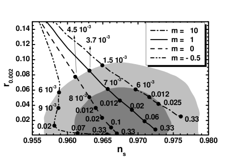
Fig. 1: Allowed curves in the $n_{\rm s}-r_{0.002}$ plane for $K=K_{i}$ ($i=1,2$) and various $m$’s (shown in the plot legend) and $r_{\pm}$’s indicated on the curves. The marginalized joint $68\%$ [$95\%$] regions from Planck, Bicep2/Keck Array and Baryon Acoustic Oscillations (BAO) data are depicted by the dark [light] shaded contours.

V Results

Imposing the conditions in Eq. (15) we restrict $\lambda/c_{-}$ and $\widehat{\phi}_{\star}$ whereas Eq. (2) constrains mainly $m$ and $r_{\pm}$. Focusing initially on $K=K_{i}$ with $i=1,2$ we present our results in Figs. 1 and 2. Namely, in Fig. 1 we compare the allowed curves in the $n_{\rm s}-r_{0.002}$ plane with the observational data plcp for $m=-1/2,0,1$ and $10$ – double dot-dashed, dashed, solid, and dot-dashed line respectively. The variation of $r_{\pm}$ is shown along each line. Note that for $m=0$ the line essentially coincides with the corresponding one in Ref. lazarides – cf. Refs. roest ; nMkin – and declines from the central $n_{\rm s}$ value in Eq. (2). On the other hand, the compatibility of the $m=1$ line with the central values in Eq. (2) is certainly impressive. For low enough $r_{\pm}$’s – i.e. $r_{\pm}\leq 10^{-4}$ – the various lines converge to the $(n_{\rm s},r_{0.002})$’s obtained within quartic inflation whereas, for larger $r_{\pm}$, they enter the observationally allowed regions and terminate for $r_{\pm}\simeq 1/3$, beyond which $\kappa_{-}$ in Eq. (13b) ceases to be well defined. Notably, this restriction provides a lower bound on $r_{0.002}$ which increases with $m$. Indeed, we obtain $r_{0.002}\gtrsim 0.0017,0.0028,0.009$ and $0.025$ for $m=-1/2,0,1$ and $10$ correspondingly. Therefore, our results are testable in forthcoming experiments cmbpol .

Repeating the same analysis for $(-1)\leq m\leq 10$ we can identify the allowed range of $r_{\pm}$ – as in Fig. 2. The allowed (shaded) region is bounded by the dashed line, which corresponds to $r_{\pm}\simeq 1/3$, and the dot-dashed and thin lines along which the lower and upper bounds on $n_{\rm s}$ and $r$ in Eq. (2) are saturated respectively. We remark that increasing $r_{\pm}$, with fixed $m$, $n_{\rm s}$ increases whereas $r$ decreases, in accordance with our findings in Fig. 1. We also infer that $r_{\pm}$ takes more natural (lower than unity) values for larger $m$’s. Fixing $n_{\rm s}$ to its central value in Eq. (2) we obtain the solid line along which we get clear predictions for $r$, $a_{\rm s}$ and $\widehat{m}_{\rm\delta\phi}$. Namely,

$$0.18\lesssim m\lesssim 10\>\>\>\mbox{and}\>\>\>1/3\gtrsim{r_{\pm}}\gtrsim 3.5\cdot 10^{-3};$$ (18a)

$$0.4\lesssim{r/0.01}\lesssim 7.6\>\>\>\mbox{and}\>\>\>5.4\lesssim-a_{\rm s}/10^{-4}\lesssim 6~{}~{}~{}~{}~{}~{}~{}~{}~{}$$ (18b)

with $2.4\cdot 10^{-8}\lesssim\widehat{m}_{\rm\delta\phi}\lesssim 8.7\cdot 10^{-6}$. Since the resulting $|a_{\rm s}|$ remains sufficiently low, our models are consistent with the fitting of data with the $\Lambda$CDM+$r$ model plcp . Finally, the $\widehat{m}_{\rm\delta\phi}$ range lets open the possibility of non-thermal leptogenesis ntlepto if we introduce a suitable coupling between $\bar{\Phi}$ and the right-handed neutrinos – see e.g. Refs. fhi1 ; nmH .

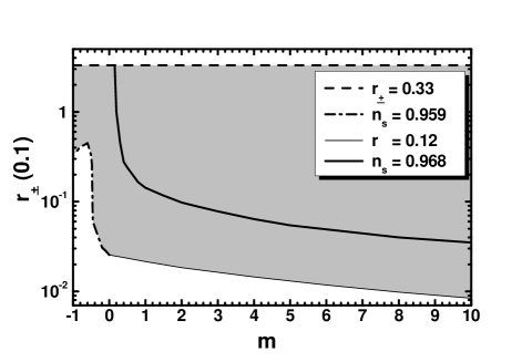
Fig. 2: Allowed (shaded) region in the $m-r_{\pm}$ plane for $K=K_{i}$. The conventions adopted for the various lines are also shown.

Had we employed $K=K_{i+2}$, the various lines in Fig. 1 and the allowed regions in Fig. 2 would have been extended until $r_{\pm}\simeq 1/2$. This bound would have yielded $r_{0.002}\gtrsim 0.0012,0.002,0.0066$ and $0.023$ for $m=-1/2,0,1$ and $10$ correspondingly, which are a little lower than those designed in Fig. 1. The lower bounds of $m$, $r_{\pm}$ and $r$ in Eqs. (18a) and (18b) become $0.19$, $1/2$, and $0.003$, the upper bound on $\widehat{m}_{\rm\delta\phi}$ moves on to $1.3\cdot 10^{-5}$ whereas the bounds on $(-a_{\rm s})$ remain unaltered.

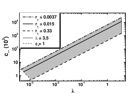
Fig. 3: Allowed (shaded) region in the $\lambda-c_{-}$ plane for $K=K_{i}$ (with $i=1,2$) and $m=1$. The conventions adopted for the various lines are also shown.

Although $\lambda/c_{-}$ is constant in our setting for fixed $r_{\pm}$ and $m$, the amplitudes of $\lambda$ and $c_{-}$ can be bounded. This fact is illustrated in Fig. 3 where we display the allowed (shaded) area in the $\lambda-c_{-}$ plane focusing on the $m=1$ case. We observe that for any $r_{\pm}$ between its minimal ($0.0037$) and maximal ($1/3$) value – depicted by bold dot-dashed and dashed lines – there is a lower bound – represented by a faint dashed line – on $c_{-}$, above which $\phi_{\star}<1$. Consequently, our proposal can be stabilized against corrections from higher order terms – e.g., $(\bar{\Phi}\Phi)^{l}$ with $l>1$ in Eq. (1). The perturbative bound $\lambda=3.5$ limits the region at the other end along the thin solid line. Plotted is also the solid line for $r_{\pm}=0.015$ which yields $n_{\rm s}=0.968$. The corresponding $r=0.043$ turns out to be impressively close to its central value in Eq. (2).

VI The Effective Cut-Off Scale

The fact that $\widehat{\phi}$ in Eq. (14a) does not coincide with $\phi$ at the vacuum of the theory – contrary to the pure nMHI cutoff ; riotto – assures that the corresponding effective theories respect perturbative unitarity up to $m_{\rm P}=1$ although $c_{-}$ may take relatively large values for $\phi_{\star}<1$ – see Fig. 3. To clarify further this point, we analyze the small-field behavior of our models in the EF for $m=1$. We focus on the second term in the r.h.s of Eq. (6a) for $\mu=\nu=0$ and we expand it about $\langle{\phi}\rangle=M\ll 1$ in terms of $\widehat{\phi}$. Our result is written as

$$J^{2}\dot{\phi}^{2}\simeq\left(1+3Nr_{\pm}^{2}\widehat{\phi}^{2}-5Nr_{\pm}^{3}\widehat{\phi}^{4}+\cdots\right)\dot{}\widehat{\phi}^{2}.$$ (19a)

Expanding similarly $$\widehat{V}_{\rm HI} \widehat{\phi}$$, see Eq. (9a), in terms of we have

$$\widehat{V}_{\rm HI}\simeq\frac{\lambda^{2}\widehat{\phi}^{4}}{16c_{-}^{2}}\left(1-2r_{\pm}\widehat{\phi}^{2}+3r_{\pm}^{2}\widehat{\phi}^{4}-\cdots\right).$$ (19b)

Similar expressions can be obtained for the other $m$’s too. Given that the positivity of $\kappa_{-}$ in Eq. (13a) entails $r_{\pm}\lesssim 1/N<1$, we can conclude that our models do not face any problem with the perturbative unitarity up to $m_{\rm P}$.

VII Conclusions and Perspectives

The feasibility of inflating with a superheavy Higgs field is certainly an archetypal open question. We here outlined a fresh look, identifying a class of Kähler potentials in Eqs. (4a) – (4d) which can cooperate with the superpotential in Eq. (1) and lead to the SUGRA potential $\widehat{V}_{\rm HI}$ collectively given by Eq. (9a). Prominent in the proposed Kähler potentials is the role of a shift-symmetric quadratic function $F_{-}$ in Eq. (3) which remains invisible in $\widehat{V}_{\rm HI}$ while dominates the canonical normalization of the Higgs-inflaton. Using $0.18~{}[0.19]\leq m\leq 10$ and confining $r_{\pm}$ to the range $(3.5\cdot 10^{-3}-1/N)$ where $N=3$ [$N=2$] for $K=K_{i}$ [$K=K_{i+2}$] – with $i=1,2$ –, we achieved observational predictions which may be tested in the near future and converge towards the “sweet” spot of the present data. These solutions can be attained even with subplanckian values of the inflaton requiring large $c_{-}$’s and without causing any problem with the perturbative unitarity. It is gratifying, finally, that our proposal remains intact from radiative corrections, the Higgs-inflaton may assume ultimately its v.e.v predicted by the gauge unification within MSSM, and the inflationary dynamics can be studied analytically and rather accurately.

As a last remark, we would like to point out that, although we have restricted our discussion to the $G_{\rm GUT}=G_{\rm SM}\times U(1)_{B-L}$ gauge group, kinetically modified nMHI has a much wider applicability. It can be realized, employing the same $W$ and $K$’s within other SUSY GUTs too based on a variety of gauge groups – such as the left-right fhi2 , the Pati-Salam nmH , or the flipped $SU(5)$ group fhi2 – provided that $\Phi$ and $\bar{\Phi}$ consist a conjugate pair of Higgs superfields so that they break $G_{\rm GUT}$ and compose the gauge invariant quantities $F_{\pm}$. Moreover, given that the term $\lambda M^{2}S/4$ of $W$ in Eq. (1) plays no role during nMHI, our scenario can be implemented by replacing it with $\kappa S^{3}$ and identifying $\Phi$ and $\bar{\Phi}$ with the electroweak Higgs doublets $H_{u}$ and $H_{d}$ of the next-to-MSSM linde1 . In this case we have to modify the shift symmetry in Eq. (5), following the approach of Ref. shiftHI , consider the soft SUSY breaking terms to obtain the radiative breaking of $G_{\rm SM}$ and take into account the renormalization-group running of the various parameters from the inflationary up to the electroweak scale in order to connect convincingly the high- with the low-energy phenomenology. In all these cases, the inflationary predictions are expected to be quite similar to the ones obtained here, although the parameter space may be further restricted. The analysis of the stability of the inflationary trajectory may be also different, due to the different representations of $\Phi$ and $\bar{\Phi}$. Since our main aim here is the demonstration of the kinetical modification on the observables of nMHI, we opted to utilize the simplest GUT embedding.

References

A.H. Guth, Phys. Rev. D 23, 347 (1981); A.D. Linde, Phys. Lett. B 108, 389 (1982); A. Albrecht and P.J. Steinhardt, Phys. Rev. Lett. 48, 1220 (1982).

D.S. Salopek, J.R. Bond and J.M. Bardeen, Phys. Rev. D 40, 1753 (1989); J.L. Cervantes-Cota and H. Dehnen, Phys. Rev. D 51, 395 (1995) [astro-ph/9412032].

M. Arai, S. Kawai, and N. Okada, Phys. Rev. D 84,1 23515 (2011) [arXiv:1107.4767]; K. Nakayama and F. Takahashi, J. Cosmol. Astropart. Phys. 05, 035 (2012) [arXiv: 1203.0323]; M.B. Einhorn and D.R.T. Jones, J. Cosmol. Astropart. Phys. 11, 049 (2012) [arXiv:1207.1710]; L. Heurtier, S. Khalil, and A. Moursy, J. Cosmol. Astropart. Phys. 10, 045 (2015) [arXiv:1505.07366].

C. Pallis and N. Toumbas, J. Cosmol. Astropart. Phys. 12, 002 (2011) [arXiv:1108.1771].

M. Arai, S. Kawai, and N. Okada, Phys. Lett. B 734, 100 (2014) [arXiv:1311.1317].

G. Lazarides and C. Pallis, J. High Energy Phys. 11, 114 (2015) [arXiv:1508.06682].

G.R. Dvali, Q. Shafi, and R.K. Schaefer, Phys. Rev. Lett. 73, 1886 (1994) [hep-ph/9406319].

C. Pallis and Q. Shafi, Phys. Lett. B 725, 327 (2013) [arXiv:1304.5202].

M. Bastero-Gil, S.F. King, and Q. Shafi, Phys. Lett. B 651, 345 (2007) [hep-ph/0604198].

M. Civiletti, C. Pallis, and Q. Shafi, Phys. Lett. B 733, 276 (2014) [arXiv:1402.6254].

S. Antusch et al., J. High Energy Phys. 08, 100 (2010) [arXiv:1003.3233]; J. Ellis, T.E. Gonzalo, J. Harz, and W.C. Huang, J. Cosmol. Astropart. Phys. 03, 039 (2015) [arXiv:1412.1460].

J.L. Cervantes-Cota and H. Dehnen, Nucl. Phys. B442, 391 (1995) [astro-ph/9505069]; F.L. Bezrukov and M. Shaposhnikov, Phys. Lett. B 659, 703 (2008) [arXiv:0710.3755].

M.B. Einhorn and D.R.T. Jones, J. High Energy Phys. 03, 026 (2010) [arXiv:0912.2718]; H.M. Lee, J. Cosmol. Astropart. Phys. 08, 003 (2010) [arXiv:1005.2735]; S. Ferrara et al., Phys. Rev. D 83, 025008 (2011) [arXiv:1008.2942].

I. Ben-Dayan and M.B. Einhorn, J. Cosmol. Astropart. Phys. 12, 002 (2010) [arXiv:1009.2276].

J.L.F. Barbon and J.R. Espinosa, Phys. Rev. D 79, 081302 (2009) [arXiv:0903.0355]; C.P. Burgess, H.M. Lee, and M. Trott, J. High Energy Phys. 07, 007 (2010) [arXiv:1002. 2730].

A. Kehagias, A.M. Dizgah, and A. Riotto, Phys. Rev. D 89, 043527 (2014) [arXiv:1312.1155].

C. Pallis, Phys. Rev. D 91, 123508 (2015) [arXiv:1503.05 887]; C. Pallis, PoS PLANCK 2015, 095 (2015) [arXiv:15 10.02306].

P.A.R. Ade et al. [Planck Collaboration], arXiv:1502.02114.

P.A.Ade et al. [Bicep2 and Planck Collaborations], Phys. Rev. Lett. 114, 101301 (2015) [arXiv:1502.00612].

J. Ellis, D.V. Nanopoulos and K.A. Olive, Phys. Rev. Lett.  111, 111301 (2013); Erratum-ibid.  111, no. 12, 129902 (2013) [arXiv:1305.1247].

R. Kallosh, A. Linde, and D. Roest, Phys. Rev. Lett. 112 (2014) 011303 [arXiv:1310.3950].

M. Kawasaki, M. Yamaguchi and T. Yanagida, Phys. Rev. Lett. 85, 3572 (2000) [hep-ph/0004243].

R. Kallosh, A. Linde, and D. Roest, J. High Energy Phys. 08, 052 (2014) [arXiv:1405.3646]; C. Pallis, J. Cosmol. Astropart. Phys. 10, 058 (2014) [arXiv:1407.8522].

P. Creminelli et al., arXiv:1502.01983.

G. Lazarides and Q. Shafi, Phys. Lett. B 258, 305 (1991); K. Kumekawa, T. Moroi, and T. Yanagida, Prog. Theor. Phys. 92, 437 (1994) [hep-ph/9405337].