Stochastic Particle Flow for Nonlinear High-Dimensional Filtering Problems

Abstract

A series of novel filters for probabilistic inference that propose an alternative way of performing Bayesian updates, called particle flow filters, have been attracting recent interest. These filters provide approximate solutions to nonlinear filtering problems. They do so by defining a continuum of densities between the prior probability density and the posterior, i.e. the filtering density. Building on these methods’ successes, we propose a novel filter. The new filter aims to address the shortcomings of sequential Monte Carlo methods when applied to important nonlinear high-dimensional filtering problems. The novel filter uses equally weighted samples, each of which is associated with a local solution of the Fokker-Planck equation. This hybrid of Monte Carlo and local parametric approximation gives rise to a global approximation of the filtering density of interest. We show that, when compared with state-of-the-art methods, the Gaussian-mixture implementation of the new filtering technique, which we call Stochastic Particle Flow, has utility in the context of benchmark nonlinear high-dimensional filtering problems. In addition, we extend the original particle flow filters for tackling multi-target multi-sensor tracking problems to enable a comparison with the new filter.

1 Introduction

Stochastic filtering in high-dimensional spaces is a challenging estimation task because of two fundamental issues:

• The curse of dimensionality. In a statistical experiment, as the sample space’s dimensionality increases a finite number of realizations can only populate the space to an increasingly sparse extent [1]. This issue makes it challenging to use approximation based on realizations of the state.

• The infinite number of parameters required to describe a general probability density on a continuous state space. Such a density, in common with any other real function, can always be exactly described using a power series with infinitely many terms. In all but a very few cases, where the density is known to have a specific parametric form, using a finite set of parameters is necessarily an approximation to this complete description. The fidelity of such approximations falls rapidly as dimension increases. This issue makes it challenging to define a parameterization that uses a number of parameters that scales only gently with dimension.

The development of the vast majority of practical filters focuses on how to accurately represent generic probability densities. However, in the view of the authors, relatively few filters are systematically developed with the explicit intent of efficiently expressing densities in high-dimensional spaces. There does appear to be a consensus that the statistical efficiency associated with expressing high-dimensional filtering densities can be improved by simulating tempering distributions [2, 3, 4, 5]. Such approaches involve introducing intermediate distributions such that it is easier to migrate between these intermediate distributions than it is to migrate directly from the prior to the posterior. The use of such intermediate distributions stabilizes the sampling procedure and maintain the variance of the Monte Carlo weights at an acceptable level. Bickel et al. [6] considered, in the context of a bootstrap particle filter, the number of intermediate distributions needed to use such tempering successfully. They prove that, as the dimensionality increases, the number of intermediate distributions needed to accurately represent a high-dimensional density becomes practically infinite. This implies that considering a continuum, i.e. infinite number, of intermediating distributions [4] might be the basis of a successful approach. This implication is corroborated by the reported success of Markov chain Monte Carlo (MCMC) algorithms that populate high-dimensional state spaces efficiently using approximations of problem-specific continuous-time processes [7, 8, 9, 10].

Techniques for continuous-time processes stem from the seminal work by Stratonovich [11], Kushner [12] and Zakai [13] on filtering theory. The most popular instance of such filters is the so-called Kalman-Bucy filter [14], the continuous-time counterpart of the Kalman filter. More general filters directly approximate solutions to the Kushner-Stratonovich equation either by a finite-dimensional density parameterization [15, 16] or by Monte Carlo methods [17, 18, 19]. Other important finite-order filters that appeal to an unusual formalism of multiple stochastic integrals [20, 21] are worth mentioning as well.

Continuous-time filtering may be seen by some as an idealized problem of limited practical utility. However, recent research [22, 23] has shown that continuous-time filtering can offer key insights into the fundamental principles necessarily associated with successful filtering in high-dimensions: the effects of local, continuous spatial properties of the observation process need to be incorporated in the solution. As identified by Bickel et al. [6], the information in the data gives rise to the notion of the effective dimension of the space. It is this effective dimension, and not the dimension of the state space itself, that actually affects the statistical efficiency of inference algorithms. This implies that tempering only addresses part of the problem, remaining the local observation properties to be incorporated. Recently, based on a principled approach, Rebeschini & van Handel [23] proposed to decompose the state space into separate blocks. The global solution to the inference problem is then constructed by combining the local solutions for each of the blocks. The paper goes on to demonstrate that, by using the decay of correlations property, it is possible to develop particle filters based on local solutions in such a way that the approximation error does not depend on the dimension of the state space.

Largely independently, the idea of filtering via a continuum of intermediate distributions seems to have its appeal revigorated as several new methods have been proposed for progressive Bayesian updates, whose continuity is considered in the limit, aiming to gradually introduce the effect of each observation. Those filters have emerged either in a variational, ensemble-based, or sequential Monte Carlo framework. In the variational framework, the new methods presented in [24, 25, 26] pose the filtering problem as a multi-step optimization problem for which the cost function is an approximated distance between a parameterised density and the actual filtering density. In the ensemble-based framework, the methods [27, 28, 29] are focused on data assimilation problems and apply ideas of optimal transport along with continuous-time filtering to generate multiple independent solutions that are combined to obtain a single solution of an inference problem. The methods in the sequential Monte Carlo framework explore extensions or alternatives to particle filters (e.g., [30, 31, 32, 33, 34]), or simply capitalize on techniques for properly choosing a sequence of bridging importance densities (e.g., [3, 4, 5, 35]), carrying on the intent to overcome the widely known problem of particle filters called degeneracy or collapse of weights [36, 37, 38, 39].

Among those methods one in particular has recently attracted interest in an Engineering context where it has been described as particle flow. The performance that has been reported is remarkable and the literature is extensive with several variants having been developed over recent years (see, for example, [32, 40, 41, 42, 43]). The development of particle flow draws on analogies to problems that arise in Fluid Dynamics and Electromagnetism. These filters flow probability masses (particles) from a prior probability space to one that is updated according to a set of measurements without the need to perform a Bayesian update explicitly. All particle flow algorithms explore the concept of a homotopy between the prior and posterior probability spaces, implicitly describing a joint measure that couples the prior and posterior probability measures. This idea is in the heart of the Kantorovich’s optimal tranportation problem [44] that, by evoking deterministic transport maps for very simple cost functions and dynamic constraints, yields an essential explanation on why original particle flow methods work well based on deterministic rules to flow the particles.

When the sequential filtering problem involves non-compactly supported densities, solving it via deterministic (optimal) transport is not straightforward. A solution would require either a non-trivial approximation of the highly nonlinear Monge-Ampère equation [45] or adapting classical solutions constructed for measures on bounded sets [46, 47]. In these approaches, severe technical difficulties may arise and not all the effects on the estimation errors are clearly known. A continuously evolving, exact, optimal transport map would require a complete description, at all time instants, of an embedding dynamic field that induces a transference plan to correctly move particles. If the posterior density could be completely characterized beforehand then the optimal transport problem could be numerically solved by the multiple-step augmented-Lagrangian optimization method as proposed by Benamou & Brenier [48]. However, detailed knowledge of the posterior would imply a direct answer to the filtering problem. As an alternative, theoretically speaking, a complete description of the optimal field could be achieved by solving the Monge-Ampère equation for any possible location of particles on the state space. Notwithstanding, the Monge-Ampère equation admits exact solutions only for few particular cases [45] and would also require a thorough description of the posterior density in advance.

In this scenario, one feasible approach is that advocated by particle flow methods, which take simplifying assumptions on the embedding dynamic field in order to avoid both optimization over a parametric class of transport maps and explicit solution of the associated elliptic partial differential equation. However, in our experience, these symplifying assumptions result in approximated filtering densities providing accurate estimates for the first-order moment but estimates for second and higher-order moments whose quality is highly dependent on the problem and algorithm settings (e.g., [49]). In practice, particle flow methods address this latter issue by either relying on a companion filter [50, 51] or using the sample covariance matrix with shrinkage and Tikhonov regularization [52] to be able to estimate the second-order moment.

We conjectured if appealing to stochastic transport could provide a new avenue for solving the filtering problem. Fortunately, a variational formulation of the Fokker-Planck equation as a gradient flow, as exposed by Jordan et al. [53], enables the precise interpretation that, if a transport operation is to be understood as a diffusion, then it minimizes the free energy functional of the process with respect to the Wasserstein metric over an admissible class of probability measures. Relying on this formulation, it is straightforward to obtain a transport rule, optimal in terms of minimizing the free energy functional, as a Langevin stochastic process. This rule is based simply on the assumptions of stationarity of the filtering distribution (Gibb’s distribution) and on potential conditions, for which an embedding stationary field is exactly derived.

In this article we take into consideration the findings presented by Jordan et al. [53], incorporate the description of statistically efficient processes in high-dimensional spaces as proposed by Girolami & Calderhead [10], and incorporate local properties of the observation process to formulate a stochastic variant of particle flow. This new stochastic particle flow (SPF) involves defining a Langevin diffusion such that a posterior measure from a previous step, under a known stationary potential field, is diffused onto the current posterior measure, satisfying the Fokker-Planck equation to produce an accurate approximation of the filtered density. This process involves guiding local solutions of the Fokker-Planck equation in such a way that we construct a mixture that approximates the posterior. As we will discuss later on, the SPF method we propose is essentially built as a Gaussian sum filter (SPF-GS), nevertheless, it is possible to use a similar formulation to define an implementation strategy based on a marginal particle filter (SPF-MPF). This variant demonstrates versatility of the SPF to algorithm settings.

It is worth mentioning that our resulting SPF technique is in the same ethos as the method recently developed by Bunch & Godsill [35, 55]. However, in constrast to our approach, their method (i) is based on the homotopy between the prior and posterior spaces, (ii) assumes the particle flow is an Ornstein-Uhlenbeck process whose scaling parameter determines the rate of diffusion of samples’ paths, (iii) proposes weights that must be updated iteratively by a partial differential equation (PDE) describing how the unnormalized log-density evolves with a pseudo-time variable; (iv) is articulated as a standard (not marginal) particle filter.

The outline of the article is as follows. We begin by reviewing the stochastic filtering problem in a sequential Monte Carlo framework in Section 2. We abstract the solution in terms of a general map that could adopt any valid method to perform the filtering update. In Section 3, we present a brief overview of the original particle flow methods. We discuss their principles in order to further clarify these methods and motivate the natural step towards stochastic particle flow. In Section 4 we derive the generic SPF algorithm by describing the proposed dynamics of probability masses, describing the associated stationary solution to the Fokker-Planck equation, and constructing the stochastic flow. Algorithmic details are given and relate to how to compute the diffusion matrix, how to integrate the stochastic flow, and how to select the simulation time horizon and integration step size. We present the stochastic particle flow implementation using a Gaussian sum filter (SPF-GS) in Section 5. We achieve this by considering the posterior to be well approximated as a mixture of local solutions to the flow. Similarly, in Section 6 we show the SPF articulated as a marginal particle filter (SPF-MPF) by setting the importance density as a mixture analogous to that generated by the SPF-GS. Section 7 then illustrates the SPF’s properties by a series of toy problems, and compares the performance of the SPF and other state-of-the-art methods in the context of three instructive multi-sensor or multi-target tracking problems: multi-sensor bearing-only tracking, convoy tracking and inference on a large network of sensors (as in [56]). In the comparisons for the multi-sensor bearing-only and convoy tracking problems, we included extensions to two of the most effective (original) particle flows, namely, the Gaussian particle flow (GPF) [57] and the scaled-drift particle flow (SDPF) [54]. Finally, Section 8 concludes.

2 Sequential Monte Carlo Filtering

In this section we report the filtering framework within which the particle flows may be formalized. Let $\{\mathrm{x}_{t}\in\mathcal{X}:t\in\mathbb{R}_{+}\}$ be a sequence of states generated through time by a known continuous-time state process, modelled as a Markov process, and $\{\mathrm{y}_{t_{k}}\in\mathcal{Y}:t_{k}\in\mathbb{R}_{+},k\in\mathbb{N}\}$ be a sequence of discrete-time observations of the process generated by an observation model. In the classical filtering problem, one is required to compute the best estimate of a function of interest $\varphi$ of the state, given all observations realized up to the time instant $t_{k}$, i.e.,

$$\hat{\varphi}_{k}=\mathbb{E}\left[\varphi(\mathrm{x}_{t_{k}})|\mathrm{y}_{t_{1}},\mathrm{y}_{t_{2}},\dots,\mathrm{y}_{t_{k}}\right].$$ (2.1)

To simplify notation, we will denote all variables at discretized time instants by the time indexes $k\in\mathbb{N}$, and write $\mathrm{y}_{1:k}^{\vphantom{(i)}}\triangleq\{\mathrm{y}_{1}^{\vphantom{(i)}},\mathrm{y}_{2}^{\vphantom{(i)}},\dots,\mathrm{y}_{k}^{\vphantom{(i)}}\}$. Now consider a set of particles $\{\mathrm{x}_{k-1}^{(i)},w_{k-1}^{(i)}:\,i=1,\,\dots,\,N\}$ constituting samples that can be used to approximate a filtering probability density $p(\mathrm{x}_{k-1}|\mathrm{y}_{1:k-1})$ by means of a Monte Carlo measure satisfying

$$\sum_{i=1}^{N}w_{k-1}^{(i)}\delta(\mathrm{x}_{k-1}^{\vphantom{(i)}}-\mathrm{x}_{k-1}^{(i)})\overset{\vphantom{\tfrac{}{}}{\scriptstyle N\rightarrow\infty}}{\longrightarrow}p(\mathrm{x}_{k-1}^{\vphantom{(i)}}|\mathrm{y}_{1:k-1}^{\vphantom{(i)}}),$$ (2.2)

to represent the convergence as follows for any test function $\varphi:\mathcal{X}\rightarrow\mathbb{R}$:

$$\sum_{i=1}^{N}w_{k-1}^{(i)}\varphi(\mathrm{x}_{k-1}^{(i)})\overset{\vphantom{\tfrac{}{}}{\scriptstyle N\rightarrow\infty}}{\longrightarrow}\int_{\mathcal{X}}\varphi(\mathrm{x}_{k-1}^{\vphantom{(i)}})p(\mathrm{x}_{k-1}^{\vphantom{(i)}}|\mathrm{y}_{1:k-1}^{\vphantom{(i)}})d\mathrm{x}_{k-1}^{\vphantom{(i)}}\quad\text{almost surely}.$$ (2.3)

Given a new observation obtained at instant $k$, one wishes to find a procedure to transform the set of particles $\{\mathrm{x}_{k-1}^{(i)},w_{k-1}^{(i)}\}$ into a new set of particles $\{\mathrm{x}_{k}^{(i)},w_{k}^{(i)}:\,i=1,\,\dots,\,N\}$ that incorporates the effect of the latest observation in order to estimate the filtered entity as

$$\hat{\varphi}_{k}\approx\sum_{i=1}^{N}w_{k}^{(i)}\varphi(\mathrm{x}_{k}^{(i)}).$$ (2.4)

In theory, the filtering problem in the sequential Monte Carlo form can be solved by any map $\mathcal{T}:\mathcal{X}\times\mathcal{Y}\rightarrow\mathcal{X}^{\prime}$, $\mathcal{T}\in\mathcal{C}^{1}(\mathbb{R}^{n_{x}})\times\mathcal{C}^{0}(\mathbb{R}^{n_{y}})$, where $\left|\mathcal{X}^{\prime}\right|=\left|\mathcal{X}\hphantom{{}^{\prime}}\right|$, that implements

$$\mathrm{x}_{k}^{(i)} \coloneqq \mathcal{T}(\mathrm{x}_{k-1}^{(i)},\mathrm{y}_{k}^{\vphantom{(i)}});\,i=1,\,\dots,\,N;$$ (2.5)

$$w_{k}^{(i)} \coloneqq \det\mathcal{J}_{\mathrm{x}_{k-1}}\left[\mathcal{T}\right]^{-1}w_{k-1}^{(i)};$$ (2.6)

where $\mathcal{J}_{\mathrm{x}_{k-1}}\left[.\right]$ is the Jacobian matrix with respect to $\mathrm{x}_{k-1}$, and such that

$$\sum_{i=1}^{N}w_{k}^{(i)}\delta(\mathrm{x}_{k}^{\vphantom{(i)}}-\mathrm{x}_{k}^{(i)})\overset{\vphantom{\tfrac{}{}}{\scriptstyle N\rightarrow\infty}}{\longrightarrow}p(\mathrm{x}_{k}^{\vphantom{(i)}}|\mathrm{y}_{1:k}^{\vphantom{(i)}}).$$ (2.7)

Although most practical filters implement the mapping (2.5) in terms of discrete Bayesian updates, there should be no objection to the general idea of considering the map $\mathcal{T}$ as a transform continuous in time within $t_{k-1}<t\leq t_{k}$. This idea establishes the basis for the particle flow filters.

3 Particle Flow

This section aims to present a brief overview on the particle flow methods, to discuss their principles, and to set the background for the introduction of the stochastic particle flow. The key idea of the particle flow is to transfer a set of probability masses by an operation that transports the prior probability measure onto the posterior measure. This operation realizes the measurement update smoothly in order to express a filtering entity, usually an estimate. The mechanism implied is, therefore, a filtering algorithm that avoids the need to perform a Bayesian measurement update explicitly.

Given a set of particles $\left\{\mathrm{x}^{(i)}\left(\lambda\right)\in\mathbb{R}^{n_{x}}:\,i=1,\,\dots,\,N\right\}$ dependent on a continuous pseudo-time variable $\lambda\in\left[0,1\right]$, where $n_{x}$ is the number of dimensions of the state space, and such that $\mathrm{x}_{\vphantom{k}}^{(i)}\left(0\right)=\mathrm{x}_{k-1}^{(i)}$ and $\mathrm{x}_{\vphantom{k}}^{(i)}\left(1\right)=\mathrm{x}_{k}^{(i)}$, the transformation of the particles is accomplished by solving through $0<\lambda\leq 1$ an ordinary differential equation (ODE) referred to as the flow equation

$$\frac{d\mathrm{x}}{d\lambda} = \mu\left(\mathrm{x},\lambda\right),\quad\mathrm{x}^{(i)}\left(0\right)\sim p_{0}\left(\mathrm{x}\right).$$ (3.1)

The varieties of particle flow methods rely on how one defines the flow drift $\mu\left(\mathrm{x},\lambda\right)$, which in turn depends on the assumptions made to solve the associated continuity equation

$$\frac{\partial p}{\partial\lambda} =-\nabla_{\mathrm{x}}\cdot\left(\mu\cdot p\right),\quad p\left(\mathrm{x},0\right)=p_{0}\left(\mathrm{x}\right).$$ (3.2)

The operator $\nabla_{\mathrm{x}}\cdot\left(.\right)$ is the divergence operator and the drift can be understood as a vector field $\mu\left(\mathrm{x},\lambda\right)\in\mathbb{R}^{n_{x}}$ that is not uniquely determined for a given probability density $p\left(\mathrm{x},\lambda\right)$. In the optimal transportation literature the vector field is usually determined by the constraint that it minimizes the kinetic energy. In that case, the flow equation (3.1) can be written in terms of a dynamic potential field as $\mu\left(\mathrm{x},\lambda\right)=\mathcal{M}^{-1}\nabla_{\mathrm{x}}\psi\left(\mathrm{x},\lambda\right)$ [44], where $\mathcal{M}$ is a positive-definite mass matrix, $\nabla_{\mathrm{x}}$ is the gradient operator, and $\psi\left(\mathrm{x},\lambda\right)$ is a dynamic potential function that satisfies the elliptic PDE

$$\nabla_{\mathrm{x}}\cdot\left(p\left(\mathrm{x},\lambda\right)\mathcal{M}^{-1}\nabla_{\mathrm{x}}\psi\left(\mathrm{x},\lambda\right)\right)=-\partial_{\lambda}p\left(\mathrm{x},\lambda\right).$$ (3.3)

An exact solution to equation (3.3) has been derived by Reich [27] considering Gaussian likelihood functions. In more general settings, if the target posterior density $\pi\left(\mathrm{x}\right)$ could be thoroughly characterized in advance, the numerical solution to this problem could be achieved by the multiple-step augmented-Lagrangian optimization method as proposed by Benamou & Brenier [48]. However, availability of a detailed description of the posterior density would constitute a direct answer to the filtering problem. Similarly, the well known flow constructed by Dacorogna & Moser [47], appropriate for mapping measures on bounded open sets, could be adapted for problems involving non-compactly supported densities as the solution of the $p$-Laplacian equation [58]

$$\nabla_{\mathrm{x}}\cdot\left(a\left(\mathrm{x},\lambda\right)\nabla_{\mathrm{x}}\vartheta\left(\mathrm{x},\lambda\right)\right)=\pi\left(\mathrm{x}\right)-p\left(\mathrm{x},\lambda\right),$$ (3.4)

where $p\left(\mathrm{x},\lambda\right)$ and $\pi\left(\mathrm{x}\right)$ are the intermediate and target densities respectively. Function $a\left(\mathrm{x},\lambda\right)\geq 0$, ${a\left(\mathrm{x},\lambda\right)\in\mathbb{L}^{\infty}}$ ($\mathbb{L}^{\infty}$-space), is a Lagrange multiplier that scales the distance of optimal transportation, whereas the term $\nabla_{\mathrm{x}}\vartheta\left(\mathrm{x},\lambda\right)$ gives the direction of optimal tranportation. As mentioned before, these transport-based solutions are not straightforwardly applicable to filtering problems as they would require anticipative approximations of the target probability density, and the solution by Dacorogna & Moser [47] would require truncation of the involved densities to bound their support.

Indeed original particle flows do not follow the classical transport-based methodology but rather take simplifying assumptions on the dynamic potential field, avoiding the complexity of solving the elliptic PDEs (3.3) and (3.4). Specifically, the particle flows are derived from a programmed sequence of a dynamic potential field that roughly solves the equation (3.2). As examples we refer the reader to the incompressible particle flow [32], the Gaussian or exact particle flow [57], and the non-zero “diffusion” particle flow [54], which is not actually a diffusion, but simply takes into account a diffusion term to scale and/or offset the drift term.

In a closely related problem, as an alternative to the solution of elliptical equations or to original particle flows, it is possible to demonstrate that if the drift solves the continuity equation (3.2), under a stationary potential field (conservative) related to an invariant, locally log-concave density of the form ${p\left(\mathrm{x},T\right)=\pi\left(\mathrm{x}\right)\propto\exp\left(-\psi\left(\mathrm{x}\right)\right)}$, then the flow (3.1) produces the maximum-a-posteriori (MAP) estimate, $\hat{\mathrm{x}}_{MAP}$, after an appropriate time horizon $\lambda\geq T$ (see Theorem 12 in the Appendix A.2). A similar concept is used in optimization algorithms based on gradient descent. An evident problem with this approach is that, regardless of providing a MAP estimate, it is unable to capture higher-order aspects of a target posterior density. Thus, under the assumption of a stationary potential field, a stochastic particle flow seems suitable to describe a filtering density precisely up to an arbitrary moment order, by following the dynamics of a diffusion that minimizes the free energy functional (see [53] for details). Such stochastic flow would propagate a probability density according to the Fokker-Planck equation. This observation becomes fundamental when we note that, loosely speaking, obtaining a precise approximation of a stationary potential field requires less effort than obtaining a sequence of accurate approximations of a dynamic potential field. In this context, approximating a dynamic potential field forms the basis for the classical transport methodology (e.g., [27]).

4 Stochastic Particle Flow

This section derives stochastic particle flow based on a stationary solution to the Fokker Planck equation. We capitalize on the fact that, under certain conditions on the drift and diffusion terms of a stochastic process, there is a stationary solution that satisfies a variational principle, minimizing a certain convex free energy functional over an admissible class of probability densities. The Fokker–Planck equation is shown to follow the direction of steepest descent of the associated free energy functional [53] at each instant of time, rendering a process where the entropy is maximized, i.e., a diffusion.

In Section 4.1 we set dynamics for stochastic particle flow. Section 4.2 derives the stationary solution to the Fokker-Planck equation such that the particles follow the Langevin dynamics. In Section 4.3 we show how to specify the Langevin dynamics to solve the specific problem of interest. In Section 4.4 we discuss the interpretation of and possible choices for the diffusion matrix; in Section 4.5 we present the integration methods used to sample from the Langevin dynamics; and in Section 4.6 we discuss criteria for choosing the algorithm’s parameters (the step size and time horizon).

4.1 Dynamics of Particles

Assuming that a set of particles $\left\{\mathrm{x}^{(i)}\left(\lambda\right):\,i=1,\,\dots,\,N\right\}$ follows a diffusion process $\left\{X_{\lambda}\right\}_{\lambda\geq 0}$ when subject to a Bayesian measurement update, the dynamics of the particles can, in general, be described by the Îto stochastic differential equation

$$dX_{\lambda}=\mathrm{\mu}\left(X_{\lambda},\lambda\right)d\lambda+\mathrm{\sigma}\left(X_{\lambda},\lambda\right)dW_{\lambda},\quad X_{0}=X\left(0\right);$$ (4.1)

such that the associated probability distribution, $p\left(\mathrm{x},\lambda\right)$, is continuously evolving with respect to the pseudo-time variable $\lambda\in\mathbb{R}_{+}$, where $\left\{W_{\lambda}\right\}$ is a standard Brownian motion, $\mathrm{\mu}\left(X_{\lambda},\lambda\right)$ is the drift vector and $\mathrm{\sigma}\left(X_{\lambda},\lambda\right)$ is the diffusion coefficient. It is well known [59, 60] that the probability density $p\left(\mathrm{x},\lambda\right)$ of an $n_{x}$-dimensional random state vector $\mathrm{x}$ under the dynamics of (4.1) has a deterministic evolution according to the Fokker-Planck equation

$$\frac{\partial}{\partial\lambda}p\left(\mathrm{x},\lambda\right)= -\sum_{i=1}^{n_{x}}\frac{\partial}{\partial x_{i}}\left[\mu_{i}\left(\mathrm{x},\lambda\right)p\left(\mathrm{x},\lambda\right)\right]$$

$$+\frac{1}{2}\sum_{i=1}^{n_{x}}\sum_{j=1}^{n_{x}}\frac{\partial}{\partial x_{i}}\frac{\partial}{\partial x_{j}}\left[D_{ij}\left(\mathrm{x},\lambda\right)p\left(\mathrm{x},\lambda\right)\right],$$ (4.2)

$$\hphantom{+\ \ }p\left(\mathrm{x},0\right)=p_{0}\left(\mathrm{x}\right),\,\lambda\geq 0;$$

where $\mathrm{x}=[x_{1},\dots,x_{n_{x}}]^{T}$, $\mathrm{\mu}=[\mu_{1},\dots,\mu_{n_{x}}]^{T}$, and

$$D_{ij}\left(\mathrm{x},\lambda\right)=\sum_{k=1}^{n_{x}}\mathrm{\sigma}_{ik}\left(\mathrm{x},\lambda\right)\mathrm{\sigma}_{jk}\left(\mathrm{x},\lambda\right),$$ (4.3)

for an $n_{x}$-dimensional Wiener process $\left\{W_{\lambda}\right\}$. In its usual form, as described in Physics, the equation reads

$$\frac{\partial}{\partial\lambda}p=-\nabla_{\mathrm{x}}\cdot\left[\mathrm{\mu}p\right]+\frac{1}{2}\nabla_{\mathrm{x}}\cdot\left[D\nabla_{\mathrm{x}}p\right].$$ (4.4)

We assume that the diffusion coefficient $\mathrm{\sigma}$ is locally independent of $\mathrm{x}$, giving rise to a local diffusion matrix $D\left(\lambda\right)=\mathrm{\sigma}\left(\lambda\right)\mathrm{\sigma}\left(\lambda\right){}^{T}$ that is invariant to the divergence operator in the vicinity of each particle. This means that, at a given time instant, the diffusion term in (4.4) evolves at a rate proportional to the curvature of a (Riemann) manifold that is approximately constant in the neighbourhood of each particle. This assumption does not affect the generality of the concepts applied in our derivation for two reasons: it results in a stochastic particle flow that is missing a simple term, of the form ${\sigma\left(x,\lambda\right)\cdot\partial_{x}\left[\sigma\left(x,\lambda\right)\right]}$, that could be incorporated if needed; in practice, any probability density can be well approximated by a mixture of densities whose covariances are locally constant with respect to the state [61] (i.e., $\partial_{x}\left[\sigma\left(x,\lambda\right)\right]=0$ locally). Additionally, as evidenced in [10], keeping the diffusion coefficient fixed for each sampling step does not perturb the target distribution.

4.2 Stationary Solution of the Fokker-Planck Equation

A stationary solution to the equation (4.4) should satisfy

$$\frac{\partial}{\partial\lambda}p\left(\mathrm{x},\lambda\right)\overset{\vphantom{\tfrac{}{}}{\scriptstyle\lambda\rightarrow\infty}}{\longrightarrow}0.$$ (4.5)

By writting

$$\nabla_{\mathrm{x}}\cdot S\triangleq\nabla_{\mathrm{x}}\cdot\left[\mathrm{\mu}\,p\right]-\frac{1}{2}\nabla_{\mathrm{x}}\cdot\left[D\nabla_{\mathrm{x}}p\right],$$ (4.6)

the definition of the probability current becomes clear:

$$S\left(\mathrm{x},\lambda\right) =\mu\left(\mathrm{x},\lambda\right)p\left(\mathrm{x},\lambda\right)-\frac{1}{2}D\left(\lambda\right)\cdot\nabla_{\mathrm{x}}p\left(\mathrm{x},\lambda\right)$$

$$=p\left(\mathrm{x},\lambda\right)\left[\mathrm{\mathrm{\mu}\left(\mathrm{x},\lambda\right)}-\frac{1}{2}D\left(\lambda\right)\cdot\nabla_{\mathrm{x}}\log p\left(\mathrm{x},\lambda\right)\right].$$ (4.7)

Since the stationary condition requires

$$\frac{\partial}{\partial\lambda}p\left(\mathrm{x},\lambda\right)=-\nabla_{\mathrm{x}}\cdot S\left(\mathrm{x},\lambda\right)\overset{\vphantom{\tfrac{}{}}{\scriptstyle\lambda\rightarrow\infty}}{\longrightarrow}0,$$ (4.8)

the probability current is required to vanish as $\lambda\rightarrow\infty$. The probability current can only vanish if the drift $\mathrm{\mu}\left(\mathrm{x},\lambda\right)$ can be expressed as the gradient of a potential function [62], cancelling out the terms within brackets in (4.7). We write the drift as the gradient of a stationary potential function according to

$$\mathrm{\mu}\left(\mathrm{x},\lambda\right)=-\frac{1}{2}D\left(\lambda\right)\cdot\nabla_{\mathrm{x}}\Phi\left(\mathrm{x}\right).$$ (4.9)

The necessary and sufficient conditions for the existence of $\Phi\left(\mathrm{x}\right)$ are the potential conditions [62]

$$\frac{\partial\mu_{i\vphantom{j}}}{\partial x_{j}}=\frac{\partial\mu_{j}}{\partial x_{i}},\quad\forall i\neq j.$$ (4.10)

Provided that the probability current vanishes as $\nabla_{\mathrm{x}}\log p\left(\mathrm{x},\lambda\right)\rightarrow-\nabla_{\mathrm{x}}\Phi\left(\mathrm{x}\right)$, we obtain the stationary solution, $p_{st}\left(\mathrm{x}\right)$, as

$$p\left(\mathrm{x},\lambda\right)\overset{\vphantom{\tfrac{}{}}{\scriptstyle\lambda\rightarrow\infty}}{\longrightarrow}p_{st}\left(\mathrm{x}\right)=\frac{1}{Z}e^{-\Phi\left(\mathrm{x}\right)},$$ (4.11)

where

$$Z=\int_{\mathbb{R}^{n_{x}}}e^{-\Phi\left(\mathrm{x}\right)}d\mathrm{x}$$ (4.12)

must be positive and finite. We promptly recognise (4.11) as analogous to the Gibbs distribution. It is verifiable that (see, for example, [63]) the Gibbs distribution minimizes the free energy functional over all probability densities on $\mathbb{R}^{n_{x}}$. It can also be shown that the stationary solution is the first eigenfunction of the Fokker-Planck equation, corresponding to the eigenvalue zero [62].

4.3 The Stochastic Flow

The general stochastic particle flow is derived by setting the stationary solution, $p_{st}\left(\mathrm{x}\right)$, to be the target posterior density, $\pi\left(\mathrm{x}\right)=p\left(\mathrm{x}|\mathrm{y}_{1:k}\right)$, to give

$$p_{st}\left(\mathrm{x}\right) \coloneqq p\left(\mathrm{x}|\mathrm{y}_{1:k}\right),$$

$$\frac{e^{-\Phi\left(\mathrm{x}\right)}}{Z\vphantom{p\left(\mathrm{y}_{1:k}\right)}} =\frac{p\left(\mathrm{y}_{k}|\mathrm{x}\right)p\left(\mathrm{x}|\mathrm{y}_{1:k-1}\right)}{p\left(\mathrm{y}_{k}|\mathrm{y}_{1:k-1}\right)},$$

$$\Phi\left(\mathrm{x}\right) =-\log p\left(\mathrm{y}_{k}|\mathrm{x}\right)-\log p\left(\mathrm{x}|\mathrm{y}_{1:k-1}\right).$$ (4.13)

Given a valid potential function $\Phi\left(\mathrm{x}\right)$ provides the stationary solution, all potential functions of the form $\Phi\left(\mathrm{x}\right)\pm K$ for any constant $K\in\mathbb{R}$ are also valid. We can therefore choose a valid potential function in (4.13) such that $p\left(\mathrm{y}_{k}|\mathrm{y}_{1:k-1}\right)=Z$. By using equation (4.9), we obtain

$$\mu\left(\mathrm{x},\lambda\right) =-\frac{1}{2}D\left(\lambda\right)\cdot\nabla_{\mathrm{x}}\Phi\left(\mathrm{x}\right)=\frac{1}{2}D\left(\lambda\right)\cdot\nabla_{\mathrm{x}}\log\pi\left(\mathrm{x}\right)$$

$$=\hphantom{-}\frac{1}{2}D\left(\lambda\right)\cdot\left[\nabla_{\mathrm{x}}\log p\left(\mathrm{y}_{k}|\mathrm{x}\right)+\nabla_{\mathrm{x}}\log p\left(\mathrm{x}|\mathrm{y}_{1:k-1}\right)\right].$$ (4.14)

Substituting (4.14) into (4.7), it is easy to see that the probability current vanishes as $\lambda\rightarrow\infty$. Additionally, it is important to note that continuous multivariate probability densities commonly used in parametric statistics (e.g., Gaussian, Student’s t, Mises-Fisher, Pareto of first kind, Cauchy etc) satisfy the potential conditions (4.10) that suffice for $\Phi\left(\mathrm{x}\right)$ to exist.

Based on equation (4.1) and on the drift obtained from the stationary solution (4.14), the dynamics of a set of particles $\left\{\mathrm{x}^{(i)}\left(\lambda\right):\,i=1,\,\dots,\,N\right\}$ can be described by the stochastic differential equation

$$d\mathrm{x} =\mathrm{\mu}\left(\mathrm{x},\lambda\right)d\lambda+\mathrm{\sigma}\left(\mathrm{x},\lambda\right)d\mathrm{w}_{\lambda},\quad\mathrm{x}_{0}^{(i)}=\mathrm{x}_{k-1}^{(i)};$$

$$d\mathrm{x} =\frac{1}{2}D\nabla_{\mathrm{x}}\log\pi\left(\mathrm{x}\right)d\lambda+D^{\nicefrac{{1}}{{2}}}d\mathrm{w}_{\lambda};$$ (4.15)

where $\pi\left(\mathrm{x}\right)$ is the target (posterior) probability density, $\left\{\mathrm{w}_{\lambda}\right\}$ is the standard Wiener process (Brownian motion) and $D$ is the diffusion matrix. The stochastic process described by (4.15) is known in the literature to follow the Langevin dynamics and, except for few special cases, cannot be exactly simulated. Thus, the most common way to ensure the simulation provides samples from the correct target distribution, $\pi\left(\mathrm{x}\right)$, is to set the discretized dynamics as a proposal within a Markov chain Monte Carlo framework, which leads to the Metropolis-adjusted Langevin algorithm (MALA) [9].

By defining the distribution at $\lambda$ and target distribution as ${d\mathcal{P}=p_{\vphantom{1}}\left(\mathrm{x},\lambda\right)d\mathrm{x}}$ and ${d\mathcal{P}_{\pi}=\pi\left(\mathrm{x}\right)d\mathrm{x}}$ respectively, one can articulate the total-variation distance between the probability measures $\mathcal{P}\left(d\mathrm{x}\right)$ and $\mathcal{P}_{\pi}\left(d\mathrm{x}\right)$ defined on $\left(\mathbb{R}^{n_{x}},\mathscr{B}(\mathbb{R}^{n_{x}})\right)$ as $\left\|\mathcal{P}_{\vphantom{1}}-\mathcal{P}_{\pi}\right\|_{\text{TV}}$. It can be shown that (e.g., [64]), if the SDE (4.15) is integrated over a sufficiently long (finite) time horizon $T\in\mathbb{R}_{+}$, then

$$\left\|\mathcal{P}_{\vphantom{1}}-\mathcal{P}_{\pi}\right\|_{\text{TV}}= \frac{1}{2}\int_{\mathbb{R}^{n_{x}}}\left|p_{\vphantom{1}}\left(\mathrm{x},\lambda\right)-\pi\left(\mathrm{x}\right)\right|d\mathrm{x}\leq\varepsilon$$ (4.16)

for any $\lambda>T$, under a desired precision $\varepsilon$. The implication is that stochastic particle flow implements the filtering mapping (2.5) with increasing accuracy as $\lambda$ progresses.

Stochastic particle flow can be interpreted as a continuous-time filtering method in the classical sense. Under the abstraction of a continuously interpolated observation process, the method has a direct correspondence to the Kallianpur-Striebel formula and satisfies the Zakai equation as we demonstrate by the Theorem 17 and Corollary 19 in the Appendix A.2. Practically speaking, the major difference between stochastic particle flow and other Langevin-based algorithms is the way that the target density is sequentially approximated via local representations that compose a mixture. This will be discussed later in Section 5.

4.4 The Diffusion Matrix

As explained by Girolami & Calderhead [10], the space of parameterized probability density functions is endowed with a natural Riemann geometry, where the diffusion matrix arises as the inverse of a position-specific metric tensor, $G\left(\mathrm{x}\left(\lambda\right)\right)$. This metric tensor maps the distances inscribed in a Riemann manifold to distances in the Euclidean space and, therefore, constitutes a means to constrain the dynamics of any stochastic process to the geometric structure of the parametric probability space. Rao [66] showed the tensor $G\left(\mathrm{x}\left(\lambda\right)\right)$ to be the expected Fisher information matrix

$$G\left(\mathrm{x}\left(\lambda\right)\right)=-\mathbb{E}_{\mathrm{y}|\mathrm{x}}\left[\mathcal{H}_{\mathrm{x}}\left[\log p\left(\mathrm{y}|\mathrm{x}\right)\right]\right],$$ (4.17)

where $\mathcal{H}_{\mathrm{x}}\left[.\right]$ is the Hessian matrix with respect to $\mathrm{x}$. In a Bayesian context, Girolami & Calderhead [10] suggested a metric tensor that includes the prior information as

$$G\left(\mathrm{x}\left(\lambda\right)\right)=-\mathbb{E}_{\mathrm{y}|\mathrm{x}}\left[\mathcal{H}_{\mathrm{x}}\left[\log p\left(\mathrm{y}|\mathrm{x}\right)\right]\right]-\mathcal{H}_{\mathrm{x}}\left[\log p_{x}\left(\mathrm{x}\right)\right],$$ (4.18)

although many possible choices of metric for a specific manifold could be advocated. Because we are interested in local (curvature) properties of stochastic particle flow, a sensible choice for the metric tensor $G\left(\mathrm{x}\left(\lambda\right)\right)$ is the observed Fisher information matrix incorporating the prior information. In this case, the diffusion matrix becomes

$$D=G\left(\mathrm{x}\left(\lambda\right)\right)^{-1}=\left[-\mathcal{H}_{\mathrm{x}}\left[\log\pi\left(\mathrm{x}\right)\right]\right]_{\mathrm{x}=\mathrm{x}_{\lambda}}^{-1},$$ (4.19)

where the Hessian matrix is locally evaluated at $\mathrm{x}=\mathrm{x}_{\lambda}^{(i)}$ for the $i$th sample, and the resulting diffusion matrix is kept constant for each integration step to obtain the subsequent sample. A problem with this choice is that the expression (4.19) may not be strictly positive definite at specific points of the state space for some types of probability distributions (e.g., mixtures). In order to solve that problem, one could appeal to methods for regularizing the diffusion matrix such as the Tikhonov regularization, the technique to find the nearest (in terms of minimum Fröbenius norm) positive definite matrix [67], or SoftAbs [68], a technique that implements a smooth absolute transformation of the eigenvalues to map the negative-Hessian metric into a positive-definite matrix. Another possibility is adopting an empirical estimate to (4.18).

4.5 Integration Method

Among the discretization methods that could be used to integrate the SDE (4.15), we advocate the use of Ozaki’s discretization [69] of the Langevin diffusion. This is more accurate than methods based on the Euler discretization. Ozaki’s discretization is only possible for target densities that are continuously differentiable and have a smooth Hessian matrix. These requirements may be fulfilled by a solution that constitutes a superposition of conveniently parameterized local approximations to a density.

The algorithm that enables simulation from the SDE (4.15) using Ozaki’s discretization is generally called Langevin Monte Carlo with Ozaki discretization (LMCO) in the MCMC community (see [64]). Provided an appropriate time horizon, $T$, by discretizing the interval $0\leq\lambda\leq T$ into $L$ sub-intervals $\{\lambda_{0}=0,\,\lambda_{1},\,\dots\lambda_{l},\,\dots,\,\lambda_{L}=T\}$, the discretized particle flow equation using Ozaki’s method is given by

$$\mathrm{x}(\lambda_{l+1}) =\mathrm{x}(\lambda_{l})+\left(\mathrm{\mathbb{I}}_{n_{x}}-e^{-\frac{\Delta\lambda}{2}D(\lambda_{l})^{-1}}\right)D(\lambda_{l})^{2}\nabla_{\mathrm{x}}\log\pi\left(\mathrm{x}(\lambda_{l})\right)$$

$$+\left[\left(\mathrm{\mathbb{I}}_{n_{x}}-e^{-\Delta\lambda D(\lambda_{l})^{-1}}\right)D(\lambda_{l})^{2}\right]^{\nicefrac{{1}}{{2}}}\mathrm{w}_{l+1},$$ (4.20)

where $\{\mathrm{w}_{l}:l=1,\dots,L\}$ is a sequence of independent random vectors distributed according to $\mathrm{w}_{l}\sim\mathcal{N}(\mathrm{w};0_{n_{x}},\mathrm{\mathbb{I}}_{n_{x}})$. The need to compute the exponential matrices in (4.20) implies an increment in complexity typically bounded by $\mathcal{O}\left(NLn_{x}^{3}\right)$ computations, which may not be justifiable for some applications. A cheaper alternative is achieved by linearizing (4.15) in the neighbourhood of the current state, assuming $D(\lambda)$ piecewise constant in pseudo-time, transforming the linearized equation by the Laplace transform, solving it in the Laplace domain, and transforming it back. The result is

$$\mathrm{x}(\lambda_{l+1}) =\mathrm{x}(\lambda_{l})+\left(1-e^{-\frac{1}{2}\Delta\lambda}\right)D(\lambda_{l})^{\vphantom{1}}\nabla_{\mathrm{x}}\log\pi\left(\mathrm{x}(\lambda_{l})\right)$$

$$+\left(1-e^{-\Delta\lambda}\right)^{\nicefrac{{1}}{{2}}}D(\lambda_{l})^{\nicefrac{{1}}{{2}}}\mathrm{w}_{l+1},$$ (4.21)

where the exponential matrices are avoided but the exponential effect on the integration variable (time step) is kept. See Appendix B for the derivation of this latter integration rule.

It is important to note that, upon integration of the SDE (4.15) by a numerical method, convergence to the invariant distribution is no longer guaranteed for any finite step size. This is due to the first-order integration error that is introduced. When tackling difficult nonlinear filtering problems where the integration error becomes significant, a correction can be carried out by employing a Metropolis acceptance step after each integration step to ensure convergence to the invariant measure.

4.6 Selection of Time Horizon and Integration Step Size

To successfully implement stochastic particle flow, it is necessary to select an adequate time horizon, $T$, and an integration step size, $\Delta\lambda$. These parameters need to be chosen such that stationarity is reached and convergence to the invariant measure is achieved. There are several routes one could take to solve this problem with each making different assumptions about the probability measures involved and about the regularity properties of the stationary distribution. One could also pose related questions in the context of specific implementations. Answering such questions might, for example, involve selecting the time horizon and integration step size that minimizes the variance of the samples’ weights.

The view adopted here is that, since computational effort is a fundamental issue for implementing stochastic particle flow, we should choose these parameters to minimize computational effort. More specifically, we want to minimize the number of integration steps that need to be performed to achieve

$$\|\mathcal{P}_{\mathcal{\tilde{\mathcal{L}}}[\Delta\lambda],T}-\mathcal{P}_{\vphantom{\tilde{\mathcal{L}}}\pi}\|_{\text{TV}}\leq\varepsilon$$ (4.22)

for an acceptable precision level $\varepsilon$, where $\mathcal{P}_{\mathcal{\tilde{\mathcal{L}}}[\Delta\lambda],T}(d\mathrm{x})$ is the approximating probability measure achieved by sampling from the discretized Langevin stochastic process over $L=\left\lceil T/\Delta\lambda\right\rceil$ steps.

Defining near-optimal choices of these parameters for general target measures, including mixtures and highly skewed distributions, would require a more thorough study that extrapolates the scope of this work. Instead, in this paper, we propose two pragmatic approaches to choosing both the time horizon and integration step size.

Approach 1

Our first approach builds on results concerning the scaling of Langevin-based MCMC algorithms: the interested reader is referred to Roberts & Rosenthal [70] and a recent extension by Pillai et al. [71] that treat high-dimensional target measures that are not of the product form. In summary, these analyses show that the number of steps required to sample the target measure by the Metropolis-Adjusted Langevin algorithm (MALA) grows as $L\sim\mathcal{O}(n_{x}^{\nicefrac{{1}}{{3}}})$. In addition, these papers work out the optimal step size by maximizing the “speed function” or, equivalently, producing the optimal average acceptance rate. Although this optimal criterion is only applicable to algorithms that employ a Metropolis acceptance step, tuning the step size used in stochastic particle flow for an “emulated” (hypothetical) acceptance rate of interest can guide the rate of convergence (even if the accept-reject step is suppressed in practice). Abusing the methodology presented by Pillai et al. [71] and using Proposition 2.4 from Roberts et al. [72], let us denote the asymptotic acceptance probability $\alpha(l)$ as a function of a scaling parameter $l\in\mathbb{R}$, such that the speed function $h(l)$ for high-dimensional MALA can be approximated as [71]

$$h\left(l\right) =l\cdot\alpha\left(l\right)\approx l\cdot\mathbb{E}_{\pi}\left[1\wedge e^{\mathcal{N}\left(-l^{3}/4,l^{3}/2\right)}\right]$$

$$=l\cdot\left[\mathcal{N}_{\text{cdf}}\left(\frac{-l^{3}/4}{\sqrt{l^{3}/2}}\right)+\exp\left(-\frac{l^{3}}{4}+\frac{\left(\sqrt{l^{3}/2}\right)^{2}}{2}\right)\mathcal{N}_{\text{cdf}}\left(-\sqrt{l^{3}/2}-\frac{-l^{3}/4}{\sqrt{l^{3}/2}}\right)\right]$$

$$=l\cdot 2\mathcal{N}_{\text{cdf}}\left(-\sqrt{l^{3}/8}\right),$$ (4.23)

where $\mathcal{N}_{\text{cdf}}(.)$ is a standard normal cumulative distribution function (cdf). One can observe the maximum occurs at $l_{opt}\approx 1.3620$ and corresponds to the theoretical optimal acceptance rate, $\alpha(l_{opt})\approx 0.5741$.

Our approach is then based on the notion that, for a conveniently selected acceptance rate, the step size should scale as $\Delta\lambda\propto l\cdot n_{x}^{-\xi}$ such that the total number of steps is scaled as $L\propto n_{x}^{\xi}$, and the exponent $\xi$ depends on whether the Metropolis adjustment is used or not. Theoretically, if the accept-reject step is not adopted then $\xi=1$, otherwise the optimal choice is $\xi=1/3$ [71].

To exemplify the use of this approach, to produce an emulated (asymptotic) acceptance rate of $\alpha=0.80$, a stochastic particle flow should be scaled as $l\approx 2\left[-\mathcal{N}_{\text{cdf}}^{-1}\left(\alpha/2\right)\right]^{2/3}=0.8008$. Using the Langevin dynamics considered herein, if $n_{x}=10$ and $\xi=1$ then $\Delta\lambda=2l\cdot n_{x}^{-\xi}\approx 0.1602$.

If the accept-reject step is present, a criterion to stop the simulation could be established online. Various MCMC convergence diagnostic methods are applicable to this task. However, in our experience with stochastic particle flow, such approaches to online determination of convergence may indicate more steps are needed than are actually necessary to obtain good results, and so give a pessimistic view of the amount of computation required. To set the time horizon when accept-reject step is not used, we note that $T=T_{0}+L_{s}\cdot\Delta\lambda$, where $T_{0}$ is the time required to take the chain to the region of high acceptance probability (“warm-up”) and $L_{s}$ is the number of steps to explore the invariant measure. We determine both $L_{s}$ and $T_{0}$ either by presetting reasonable values, or based on the second approach to be explained next.

Approach 2

Our second approach is an extension of the method proposed by Dalalyan [64]. It is useful due to its ease of application and suitability to “nicely” measurable filtering quantities although, strictly speaking, the method is only applicable to target densities that are log-concave. The criteria are presented as follows.

Theorem 1.

Let $\Phi:\mathbb{R}^{n_{x}}\rightarrow\mathbb{R}$ be a measurable convex function satisfying

$$\int_{\mathbb{R}^{n_{x}}}\exp\{-\Phi\left(\mathrm{x}\right)\} <\infty,$$ (4.24)

$$\begin{gathered}\Phi\left(\mathrm{x}\right)-\Phi\left(\bar{\mathrm{x}}\right)-\nabla_{\mathrm{x}}\Phi\left(\bar{\mathrm{x}}\right)^{T}\left(\mathrm{x}-\bar{\mathrm{x}}\right)\end{gathered} \geq\frac{1}{2}m\left\|\mathrm{x}-\bar{\mathrm{x}}\right\|_{2}^{2},$$ (4.26)

$$\left\|\nabla_{\mathrm{x}}\Phi\left(\mathrm{x}\right)-\nabla_{\mathrm{x}}\Phi\left(\bar{\mathrm{x}}\right)\right\|_{2} \leq M\left\|\mathrm{x}-\bar{\mathrm{x}}\right\|_{2},\quad\forall\mathrm{x},\bar{\mathrm{x}}\in\mathbb{R}^{n_{x}},$$ (4.27)

for two existing positive constants $m$ and $M$. Let $\bar{\mathrm{x}}\in\mathbb{R}^{n_{x}}$ be the global minimum of $\Phi(\mathrm{x})$. Suppose a discrete-time Langevin Monte Carlo algorithm integrates (4.15), targeting the invariant density $\pi(\mathrm{x})\propto\exp\{-\Phi(\mathrm{x})\}$ with measure $\mathcal{P}_{\pi}(d\mathrm{x})$, and with the initial density $\nu\left(\mathrm{x}\right)=\delta(\mathrm{x}-\mathrm{x}_{\nu})$ (a probability mass initially located at $\mathrm{x}=\mathrm{x}_{\nu}$). In addition, assume that for some $\gamma\geq 1$ we have $\Delta\lambda\leq\left(\gamma M\right)^{-1}$, and $K=\sup_{\mathrm{x}}\|D(\mathrm{x})\|_{2}$ where $D_{\lambda}=D(\mathrm{x}_{\lambda})$ is the diffusion matrix. Then, for a time horizon, $T$, and step size, $\Delta\lambda$, the total-variation distance between the target measure $\mathcal{P}_{\pi}$ and the approximated measure $\mathcal{P}_{\mathcal{\tilde{\mathcal{L}}}(\Delta\lambda),T}$ furnished by the discrete-time Langevin Monte Carlo algorithm satisfies

$$\|\mathcal{P}_{\mathcal{\tilde{\mathcal{L}}}[\Delta\lambda],T}-\mathcal{P}_{\vphantom{\tilde{\mathcal{L}}}\pi}\|_{\text{TV}}\leq\frac{1}{2}\exp\left\{-\frac{1}{2}mT+\frac{n_{x}}{2}\log\left(\frac{M}{m}\right)-\log\left[\Gamma_{u}\left(\frac{n_{x}}{2},\frac{M\|\bar{\mathrm{x}}-\mathrm{x}_{\nu}\|_{2}^{2}}{2}\right)\right]\right\}\\ +\frac{1}{2}-\frac{1}{2}\exp\left\{-\frac{n_{x}}{2}\frac{M^{3}K^{4}\gamma}{48(2\gamma-1)}\left(\frac{1}{n_{x}}\|\mathrm{\bar{x}}-\mathrm{x}_{\nu}\|_{2}^{2}+2T\right)\Delta\lambda^{2}-\frac{n_{x}M^{2}K^{3}T}{16}\Delta\lambda\right\},$$ (4.28)

where $\Gamma_{u}(s,x)\triangleq\Gamma(s)^{-1}\int_{x}^{\infty}t^{s-1}e^{-t}dt$ is the upper incomplete gamma function.

Corollary 2.

Let $n_{x}\geq 2$, $\Phi$ satisfy (4.24), (4.26) and (4.27), and $\varepsilon\in(0,\nicefrac{{1}}{{2}})$ be a desired precision level. Let the time horizon $T$ and the step size $\Delta\lambda$ be defined by

$$T \geq\frac{2\log\left(1/\varepsilon\right)+n_{x}\log\left(\frac{M}{m}\right)-2\log\left[\Gamma_{u}\left(\frac{n_{x}}{2},\frac{M\|\bar{\mathrm{x}}-\mathrm{x}_{\nu}\|_{2}^{2}}{2}\right)\right]}{m},$$ (4.29)

$$\Delta\lambda \leq\frac{-\frac{T}{16}+\sqrt{\left(\frac{T}{16}\right)^{2}+\frac{\gamma}{48(2\gamma-1)}\left(\frac{1}{n_{x}}\|\mathrm{\bar{x}}-\mathrm{x}_{\nu}\|_{2}^{2}+2T\right)M^{-1}K^{-2}\left[\frac{2}{n_{x}}\log\left(\frac{1}{1-\varepsilon}\right)\right]}}{\frac{\gamma}{48(2\gamma-1)}\left(\frac{1}{n_{x}}\|\mathrm{\bar{x}}-\mathrm{x}_{\nu}\|_{2}^{2}+2T\right)MK},$$ (4.30)

where $\gamma\geq 1$. Then the resulting probability distribution of a Langevin Monte Carlo algorithm that integrates (4.15) after $L=\left\lceil T/\Delta\lambda\right\rceil$ steps, satisfies $\|\mathcal{P}_{\mathcal{\tilde{\mathcal{L}}}[\Delta\lambda],T}-\mathcal{P}_{\vphantom{\tilde{\mathcal{L}}}\pi}\|_{\text{TV}}\leq\varepsilon$.

Theorem 1 is thoroughly underpinned by the findings of Dalalyan [73], with specific settings changed to match the Langevin algorithm proposed in this paper, and both a more general bound for the time horizon and a tightened bound for the step size (to reduce computational effort). We recommend the reader interested in the proof to first refer to [73] and then follow the missing arguments for its proof in the Appendix A.1.

Corollary 2 is a direct criterion for selecting the time horizon and step size, arising from the right-hand side of the inequality (4.28) being set to be a desired precision level. It is essential to clarify that some practical issues arise here: in this form, the method holds for log-concave densities only; the positive constants, $m$ and $M$, are assumed known a priori; and the approximation of the filtering density is not taken into account in the error budget. Rigorously speaking, the method does not apply to more general cases. However, the method has utility as the basis of an approximate (and pragmatic) mechanism for obtaining the required parameters. In making this approximation, we explicitly acknowledge that we are assuming that:

1. The target density can be well characterized by a central tendency statistic, $\bar{\mathrm{x}}_{c}$, that replaces and roughly represents $\bar{\mathrm{x}}$ in all aspects of the analysis.

2. The initial measure is composed of a superposition of $N$ probability masses described by

   $$N^{-1}\sum_{i=1}^{N}\delta(\mathrm{x}-\mathrm{x}^{(i)})$$

   or, equivalently, an empirical distribution with mean $\mu_{\nu}$ and covariance matrix $\mathrm{V}$, spatially encompassing all initial samples (from the previous filtering iteration), which is assumed to constrain the constants $M$ and $m$ by

   $$M <\|\mathrm{V}\|_{2}/2,$$ (4.31)

   $$(\mathrm{x}^{(i)}-\bar{\mathrm{x}}_{c})^{T}\frac{m}{2}(\mathrm{x}^{(i)}-\bar{\mathrm{x}}_{c}) \geq\chi_{\text{cdf}}^{-2}(0.99,n_{x}),\quad\forall\mathrm{x}^{(i)}:\,i=1,\dots,N,$$ (4.32)

   where $\chi_{\text{cdf}}^{-2}(P,\kappa)$ is the inverse of chi-square cdf for probability $P$ and $\kappa$ degrees of freedom.

3. In accordance with Lemma 4 in [64], the constant $M$ is also constrained by

   $$\Phi(\mathrm{x}^{(i)})-\Phi(\bar{\mathrm{x}}_{c})-\nabla_{\mathrm{x}}\Phi(\bar{\mathrm{x}}_{c})^{T}(\mathrm{x}^{(i)}-\bar{\mathrm{x}}_{c}) \leq\frac{M}{2}\left\|\mathrm{x}-\bar{\mathrm{x}}_{c}\right\|_{2}^{2},\quad\forall\mathrm{x}^{(i)}:i=1,\dots,N.$$ (4.33)

4. The positive constants $M$ and $m$ can be roughly estimated by

   1. approximating the statistic $\bar{\mathrm{x}}_{c}$ of the target density (e.g., obtaining a maximum-a-posteriori estimate by optimization or an approximated mean by the EKF),

   2. inverting conditions (4.26) and (4.27), and incorporating the constraint (4.33), to give

      $$\tilde{M}= 2\sup_{i\in[1,N]}\max\left[\frac{\left\|\nabla_{\mathrm{x}}\Phi(\mathrm{x}^{(i)})-\nabla_{\mathrm{x}}\Phi(\bar{\mathrm{x}}_{c})\right\|_{2}}{2\left\|\mathrm{x}^{(i)}-\bar{\mathrm{x}}_{c}\right\|_{2}},\frac{\Phi(\mathrm{x}^{(i)})-\Phi(\bar{\mathrm{x}}_{c})-\nabla_{\mathrm{x}}\Phi(\bar{\mathrm{x}}_{c})^{T}(\mathrm{x}^{(i)}-\bar{\mathrm{x}}_{c})}{\left\|\mathrm{x}^{(i)}-\bar{\mathrm{x}}_{c}\right\|_{2}^{2}}\right],$$ (4.34)

      $$\tilde{m}= 2\inf_{i\in[1,N]}\frac{\Phi(\mathrm{x}^{(i)})-\Phi(\bar{\mathrm{x}}_{c})-\nabla_{\mathrm{x}}\Phi(\bar{\mathrm{x}}_{c})^{T}(\mathrm{x}^{(i)}-\bar{\mathrm{x}}_{c})}{\left\|\mathrm{x}^{(i)}-\bar{\mathrm{x}}_{c}\right\|_{2}^{2}},$$ (4.35)

      where all quantities can be computed from definition $\Phi\left(\mathrm{x}\right)\triangleq-\log p\left(\mathrm{y}_{k}|\mathrm{x}\right)-\log p\left(\mathrm{x}|\mathrm{y}_{1:k-1}\right)$ given an approximation to the prior pdf; the resulting values of $\tilde{M}$ and $\tilde{m}$ must also satisfy (4.31) and (4.32).

Once the positive constants $M$ and $m$ have been estimated, obtaining $T$ and $\Delta\lambda$ follows from (4.29) and (4.30) respectively. In our experience, for very simple problems, (4.29) may produce overestimated time horizons and, as a consequence, may cause (4.30) to produce underestimated step sizes for stochastic particle flow. This happens because the bound for the time horizon becomes loose, in view of Lemma 7, for initial distributions that are far from the target distribution. In simple cases, a closer approximation can by achieved by assuming 1-uniform ergodicity of the Markov chain to give

$$T\geq\frac{2\log\left(1/\varepsilon\right)+n_{x}\log R}{\tilde{m}},$$ (4.36)

for a finite $R\in\mathbb{R}_{+},$ at the cost of having to determine $R$ empirically. Similarly, for simple cases, expression (4.30) can be replaced with an empirical rule of the form

$$\Delta\lambda\leq 2\frac{\sqrt{\tilde{m}}}{\tilde{M}},$$ (4.37)

which satisfies $\Delta\lambda\leq\left(\gamma\tilde{M}\right)^{-1}$ for $\gamma\leq\left(2\sqrt{\tilde{m}}\right)^{-1}$ as required by Theorem 1, but is not guaranteed to satisfy Corollary 2.

5 Stochastic Particle Flow as a Gaussian Sum Filter

In this section we use stochastic particle flow to derive a filter that approximates the posterior probability density as a Gaussian mixture. We refer to the resulting filter as the stochastic particle flow Gaussian sum filter (SPF-GS).

5.1 The Mixture-Based Approximating Measure

Given a set of samples drawn from an importance distribution, $\left\{\mathrm{x}^{(i)}\in\mathcal{X}:\,i\in 1,\,\dots,\,N\right\}$, if one is required to solve the filtering problem by a standard Monte Carlo method, then the stochastic filter adopts the following approximation

$$\hat{\varphi} =\int_{\mathrm{\mathcal{X}}}\varphi\left(\mathrm{x}\right)\pi\left(\mathrm{x}\right)dx$$

$$\approx\int_{\mathrm{\mathcal{X}}}\varphi\left(\mathrm{x}\right)\sum_{i=1}^{N}w(\mathrm{x}^{(i)})\delta(\mathrm{x}-\mathrm{x}^{(i)})d\mathrm{x}$$

$$=\sum_{i=1}^{N}w^{(i)}\varphi(\mathrm{x}^{(i)}),$$ (5.1)

where $w(\mathrm{x}^{(i)})=w^{(i)}$ are the importance weights. Now suppose that we have access to an approximating measure $\tilde{\mathcal{P}}_{\pi}\left(d\mathrm{x}\right)$ on $(\mathcal{X},\mathscr{B}(\mathcal{X}))$ with an associated density such that $d\tilde{\mathcal{P}}_{\pi}=\tilde{\pi}d\mathrm{x}$. If the density $\tilde{\pi}$ involves a mixture of $N$ Gaussians according to

$$\tilde{\pi}\left(\mathrm{x}\right) =\sum_{i=1}^{N}w_{m}^{(i)}\mathcal{N}(\mathrm{x};\mu_{m}(\mathrm{x}^{(i)}),\Sigma_{m}(\mathrm{x}^{(i)}))$$

$$=\sum_{i=1}^{N}w_{m}^{(i)}\mathcal{N}(\mathrm{x};\mu_{m}^{(i)},\Sigma_{m}^{(i)}),$$ (5.2)

where $\{w_{m}^{(i)},\mu_{m}^{(i)},\Sigma_{m}^{(i)}\}$ are computed based on the samples $\{\mathrm{x}^{(i)}\}$, then the solution is given by

$$\hat{\varphi} =\int_{\mathrm{\mathcal{X}}}\varphi\left(\mathrm{x}\right)\pi\left(\mathrm{x}\right)d\mathrm{x}$$

$$\approx\int_{\mathrm{\mathcal{X}}}\varphi\left(\mathrm{x}\right)\sum_{i=1}^{N}w_{m}^{(i)}\mathcal{N}(\mathrm{x};\mu_{m}^{(i)},\Sigma_{m}^{(i)})d\mathrm{x}$$

$$=\sum_{i=1}^{N}w_{m}^{(i)}\int_{\mathrm{\mathcal{X}}}\varphi\left(\mathrm{x}\right)\mathcal{N}(\mathrm{x};\mu_{m}^{(i)},\Sigma_{m}^{(i)})d\mathrm{x}$$

$$=\sum_{i=1}^{N}w_{m}^{(i)}\mathbb{E}_{\mathcal{N}}\left[\varphi\left(\mathrm{x}\right)|\mu_{m}^{(i)},\Sigma_{m}^{(i)}\right].$$ (5.3)

In this setting, it is possible to prove that $\tilde{\pi}\left(\mathrm{x}\right)\rightarrow\pi\left(\mathrm{x}\right)$ as $N\rightarrow\infty$ almost surely if $\mu_{m}^{(i)}\rightarrow\mathrm{x}^{(i)}$ and $\Sigma_{m}^{(i)}\rightarrow 0$, by appealing to convergence proofs for mixture-based estimators (see [74], pages 197–199). Also, it is worth noting that this procedure is quite general in the sense that (5.2) could be replaced by a mixture of any convenient parametric distribution.

5.2 The Stochastic-Particle-Flow Gaussian Sum Filter

Building upon the results presented in the previous section, SPF-GS uses samples to propagate local Gaussian components, which can together provide an accurate approximation to the posterior probability density of the form (5.2). More specifically, given a new measurement and a set of samples and moments $\{\mathrm{x}_{k-1}^{(i)},\mu_{m,k-1}^{(i)},\Sigma_{m,k-1}^{(i)}:i=1,\dots,N\}$, the filtering procedure consists of integrating the SDE (4.15) for each particle $\mathrm{x}^{(i)}\left(\lambda\right)$ and propagating its associated moments $(\mu_{m}^{(i)}\left(\lambda\right),\Sigma_{m}^{(i)}\left(\lambda\right))$ through the interval $0<\lambda\leq T$, which corresponds to the interval $t_{k-1}<t\leq t_{k}$. The integration process is performed until one achieves the posterior set of samples and parameters $\{\mathrm{x}_{k}^{(i)},\mu_{m,k}^{(i)},\Sigma_{m,k}^{(i)}\}\coloneqq\{\mathrm{x}^{(i)}\left(T\right),\mu_{m\vphantom{k}}^{(i)}\left(T\right),\Sigma_{m\vphantom{k}}^{(i)}\left(T\right)\}$, where $\mathrm{x}_{\vphantom{k-1}}^{(i)}\left(0\right)=\mathrm{x}_{k-1}^{(i)}$, so that

$$\frac{1}{2}\int_{\mathrm{\mathcal{X}}}\left|\sum_{i=1}^{N}\frac{1}{N}\mathcal{N}(\mathrm{x};\mu_{m}^{(i)}(T),\Sigma_{m}^{(i)}(T))-\pi\left(\mathrm{x}\right)\right|d\mathrm{x} \leq\varepsilon^{\prime},$$

under a desired precision level $\varepsilon^{\prime}$ as $N\rightarrow\infty$. In practice, the integration of stochastic particle flow (4.15) over $0<\lambda\leq T$ involves multiple intermediate sampling steps that evolve the samples $\mathrm{x}^{(i)}\left(\lambda\right)$ to populate the local regions of the state space where the target distribution will be described. At the same time, the mixture components are propagated to define the local approximations and thereby the global approximation to the filtering density. A fundamental aspect of the procedure proposed herein is that, for each filtering step, the intermediate moments $(\mu_{m}^{(i)}\left(\lambda\right),\Sigma_{m}^{(i)}\left(\lambda\right))$ are initialized as departing from the corresponding samples obtained from the previous step, i.e., $\mu_{m}^{(i)}\left(0\right)\coloneqq\mathrm{x}_{k-1}^{(i)}$ and $\Sigma_{m}^{(i)}\left(0\right)\coloneqq 0_{n_{x}\times n_{x}}$, and evolved onto the local posterior moments, $\mu_{m}^{(i)}(T)$ and $\Sigma_{m}^{(i)}(T)$. In this setting, each component of the filtering mixture is associated, via Fokker-Planck equation (Langevin dynamics), with the mapping

$$\frac{1}{N}\delta(\mathrm{x}_{k-1}^{\vphantom{(i)}}-\mathrm{x}_{k-1}^{(i)})\mapsto\frac{1}{N}\mathcal{N}(\mathrm{x}_{k}^{\vphantom{(i)}};\mu_{m,k}^{(i)},\Sigma_{m,k}^{(i)}).$$ (5.4)

It is also important to highlight that we perceive the most informative approximation of the posterior from the previous iteration as provided by the set of moments from the previous iteration, $\{\mu_{m,k-1}^{(i)},\Sigma_{m,k-1}^{(i)}\}$, and not by the samples. We therefore use the previous iteration’s mixture to define the invariant target measure but samples from this mixture to integrate the SDE. In our experience, this setting is beneficial because: it avoids the bias that would result from propagating a mixture-only approximation from one filtering iteration to the next; it dismisses the need to explicitly compute mixture weights since the ergodic Markov chain that carries out (5.4) is known to converge to the invariant measure no matter where it starts [75].

More specifically, in the Langevin diffusion setting presented in Section 4, the mixture measure forms the basis of approximating the target log-density. Each mixture component from the previous filtering step enables a local approximation of the prior density as

$$\tilde{p}^{(i)}\left(\mathrm{x}_{k}^{\prime}|\mathrm{y}_{1:k-1}^{\vphantom{\prime}}\right)=\int_{\mathbb{R}^{n_{x}}}p_{t}(\mathrm{x}_{k}^{\prime\vphantom{(i)}}|\mathrm{x}_{k-1}^{\vphantom{(i)}})\mathcal{N}(\mathrm{x}_{k-1}^{\vphantom{(i)}};\mu_{m,k-1}^{(i)},\Sigma_{m,k-1}^{(i)})d\mathrm{x}_{k-1}^{\vphantom{\prime}},$$ (5.5)

where $p_{t}\left(\mathrm{x}_{k}^{\prime}|\mathrm{x}_{k-1}^{\vphantom{\prime}}\right)$ is the state-process transition kernel, and the resulting prior density is locally approximated as a Gaussian (e.g., via the Unscented Transform). Thus, provided a known likelihood function, $p\left(\mathrm{y}_{k}|\mathrm{x}\right)$, one Langevin transition kernel is computed per sample based on $\nabla_{\mathrm{x}}\log\tilde{\pi}^{(i)}(\mathrm{x})=\nabla_{\mathrm{x}}\log p\left(\mathrm{y}_{k}|\mathrm{x}\right)+\nabla_{\mathrm{x}}\log\tilde{p}^{(i)}\left(\mathrm{x}|\mathrm{y}_{1:k-1}\right)$.

We propose an approximate method to propagate the moments, $\mu_{m}(\lambda)$ and $\Sigma_{m}(\lambda)$, by linearizing the flow locally, in the neighbourhood of a probability mass located at $\mathrm{x}_{l}$. In the Appendix C we provide an argument (which we regard as useful, if not rigorous) to justify why this local flow approximation should produce acceptable errors on the propagated moments. The procedure produces a negligible error for a small state displacement given a small increment of pseudo-time, $\Delta\lambda$, so that stochastic particle flow (4.15) can be approximated within the region $\left\|\mathrm{x}-\mathrm{x}_{l}\right\|<\zeta$, for a sufficiently small $\zeta\in\mathbb{R}_{+}$, as

$$d\mathrm{x} =\frac{1}{2}D(\lambda)\nabla_{\mathrm{x}}\log\pi\left(\mathrm{x}\right)d\lambda+D(\lambda)^{\nicefrac{{1}}{{2}}}d\mathrm{w}_{\lambda},\quad\lambda\in(\lambda_{l},\lambda_{l}+\Delta\lambda],\,\mathrm{x}(\lambda_{l})=\mathrm{x}_{l};$$

$$d\mathrm{x} \approx\left[C(\mathrm{x}_{l},\lambda)\cdot\mathrm{x}+c(\mathrm{x}_{l},\lambda)\right]d\lambda+D(\lambda)^{\nicefrac{{1}}{{2}}}d\mathrm{w}_{\lambda}.$$ (5.6)

As a consequence of integrating the flow, the corresponding component moments are evolved according to the locally approximated ordinary differential equations (Appendix C)

$$\frac{d\mu_{m}^{(i)}(\lambda)}{d\lambda} =C(\mathrm{x}_{l}^{(i)})\mu_{m}^{(i)}(\lambda)+c(\mathrm{x}_{l}^{(i)}),$$ (5.7)

$$\frac{d\Sigma_{m}^{(i)}(\lambda)}{d\lambda} =C(\mathrm{x}_{l}^{(i)})\Sigma_{m}^{(i)}(\lambda)+\Sigma_{m}^{(i)}(\lambda)C^{T}(\mathrm{x}_{l}^{(i)})+D^{(i)}.$$ (5.8)

For nonlinear Gaussian problems, the locally approximated flow implies that

$$C\left(\mathrm{x}_{l},\lambda\right) =-\frac{1}{2}D(\lambda)P_{k|k-1}^{-1}$$

$$\hphantom{\,=}-\frac{1}{2}D(\lambda)\mathcal{J}_{\mathrm{x}}\left[h(\mathrm{x}_{l})\right]^{T}R_{k}^{-1}\mathcal{J}_{\mathrm{x}}\left[h(\mathrm{x}_{l})\right],$$ (5.9)

$$c\left(\mathrm{x}_{l},\lambda\right) =\hphantom{+}\frac{1}{2}D(\lambda)P_{k|k-1}^{-1}f(\mu_{m,k-1}^{\vphantom{-1}})$$

$$\hphantom{\,=}+\frac{1}{2}D(\lambda)\mathcal{J}_{\mathrm{x}}\left[h(\mathrm{x}_{l})\right]^{T}R_{k}^{-1}\mathcal{J}_{\mathrm{x}}\left[h(\mathrm{x}_{l})\right]\cdot\mathrm{x}_{l}$$

$$\hphantom{\,=}+\frac{1}{2}D(\lambda)\mathcal{J}_{\mathrm{x}}\left[h(\mathrm{x}_{l})\right]^{T}R_{k}^{-1}\left(\mathrm{y}_{k}-h(\mathrm{x}_{l})\right),$$ (5.10)

where $\mathcal{J}_{\mathrm{x}}\left[\cdot\right]$ is the Jacobian matrix with respect to the state, $f(\cdot)$ is the state process function, $h(\cdot)$ is the observation function, and where

$$P_{k|k-1} =\mathbb{E}\left[(\mathrm{x}_{k|k-1}-f(\mu_{m,k-1}))(\mathrm{x}_{k|k-1}-f(\mu_{m,k-1}))^{T}\right],$$ (5.11)

$$R_{k\hphantom{|k-1}} =\mathbb{E}\left[(\mathrm{y}_{k}-h(\mathrm{x}_{k}))(\mathrm{y}_{k}-h(\mathrm{x}_{k}))^{T}\right],$$ (5.12)

are, respectively, the covariance matrix of the prior probability density and the covariance matrix of the observation noise.

Notice that the resulting algorithm is somewhat similar to the Kalman-Bucy filter, in that it avoids an explicit discrete-time measurement update. One could also interpret the SPF-GS as a Monte-Carlo and continuous-time version of the original Gaussian sum filter [76, 77], albeit modified to explore the Riemannian geometric structure of the probability space. However, in contrast to the Gaussian sum filter (and the particle filter), the structure of the SPF-GS removes the need to explicitly compute mixture weights: it relies on multiple independent (ergodic) Markov chains that start at the samples to produce equally weighted mixture components, each describing a local version of the underlying geometric structure of the posterior measure.

The SPF-GS has features that are apparently similar to those of the Gaussian sum particle filter [78], however, in reality, these filters rely on distinct fundamental principles that make them very different. The principle of the Gaussian sum particle filter is using importance sampling to estimate the moments of a mixture’s components for approximating a target density. In contrast, the SPF-GS evolves a mixture through multiple intermediate steps by exploring the local properties of a stochastic flow in order to translate probability masses from the previous iteration to a mixture on the posterior probability space. The SPF-GS is also very different from that proposed by Terejanu et al. [79], which is a Gaussian sum filter analogous to an extended Kalman-Bucy filter, but providing an estimate of the predicted mixture weights based on an optimization procedure.

The stochastic particle flow Gaussian-sum filter (SPF-GS) is summarized in Algorithm 1. The algorithm is expressed in a quite general form, including an accept-reject step that enforces theoretical convergence to the invariant target measure. Our empirical experience indicates that having this step was often not necessary (at least in the cases we have considered). As has already been touched on, if computational efficiency is a primary goal, the SPF-GS should avoid the accept-reject step: calculating the acceptance probability requires double the number of computations of the gradients and inverted Hessian matrices. In addition, using this step requires the explicit evaluation of the kernels and target densities themselves. When the step is removed, there may be the need to deal with outliers, which can significantly affect the estimates because all components in the propagated mixture are treated as equally important. In all numerical examples studied in this paper, none adopted the Metropolis adjustment. For the high-dimensional examples, the (occasional) outliers are removed online by an empirical test to identify the samples that fall outside a credible inference region.

1 Initialization:

2 if time $k=0$ then

3       Sample $\mathrm{x}_{0}^{(i)}\sim p(\mathrm{x}_{0}^{\vphantom{(i)}}),\,\forall i=1,\dots,N$

4       Set $w_{m,0}^{(i)}\coloneqq N^{-1}$, $\mu_{m,0}^{(i)}\coloneqq\mathbb{E}_{p_{0}}\left[\mathrm{x}_{0}\right]$, $\Sigma_{m,0}^{(i)}\coloneqq\mathbb{E}_{p_{0}}\left[(\mathrm{x}_{0}-\bar{\mathrm{x}}_{0})(\mathrm{x}_{0}-\bar{\mathrm{x}}_{0})^{T}\right]$, $\forall i=1,\dots,N$

5      

6 end if

7Steps:

8 for time $k\geq 1$ do

9       Compute the time horizon $T$ and step size $\Delta\lambda$ (section 4.6)

10       Discretize the interval $0\leq\lambda\leq T$ into $L$ sub-intervals $\{\lambda_{0}=0,\,\dots\lambda_{l},\,\dots,\,\lambda_{L}=T\}$

11       Set $\mathrm{x}_{l=0}^{(i)}\coloneqq\mathrm{x}_{k-1}^{(i)}$, $\mu_{l=0}^{(i)}\coloneqq\mathrm{x}_{k-1}^{(i)}$, $\Sigma_{l=0}^{(i)}\coloneqq 0_{n_{x}\times n_{x}}$, $\forall i=1,\dots,N$

12      

13      for $l=1$ to $L$ do

14             for $i=1,\dots,N$ do

15                   Simulate

$$\mathrm{x}_{l}^{\star(i)}\leftarrow\mathrm{x}_{l-1}^{(i)}+\frac{1}{2}\int_{\lambda_{l-1}}^{\lambda_{l}}D(\mathrm{x}_{l-1}^{(i)})\nabla_{\mathrm{x}}\log\tilde{\pi}(\mathrm{x}_{l-1}^{(i)})d\lambda+\int_{\lambda_{l-1}}^{\lambda_{l}}D(\mathrm{x}_{l-1}^{(i)})^{\nicefrac{{1}}{{2}}}d\mathrm{w}_{\lambda}$$ (5.13)

16                  

17                  Compute the MH acceptance probability $\rho^{(i)}=\min\left[1,\frac{\tilde{\pi}(\mathrm{x}_{l}^{\star(i)})}{q(\mathrm{x}_{l}^{\star(i)}|\mathrm{x}_{l-1}^{(i)})}\frac{q(\mathrm{x}_{l-1}^{(i)}|\mathrm{x}_{l}^{\star(i)})}{\tilde{\pi}(\mathrm{x}_{l-1}^{(i)})}\right]$

                   /* We advocate using the Metropolis-adjustment step as practically optional, i.e., only for difficult problems. For many Engineering problems the approximation achieved by suppressing the MH step may be enough and will be more computationally efficient. */

18                   Simulate $z^{(i)}\sim\mathcal{U}(0,1)$

19                   if $z^{(i)}\leq\rho^{(i)}$ then

20                         Set $\mathrm{x}_{l}^{(i)}\leftarrow\mathrm{x}_{l}^{\star(i)}$

21                         Propagate

$$\mu_{l}^{(i)}\leftarrow\mu_{l-1}^{(i)}+\int_{\lambda_{l-1}}^{\lambda_{l}}\left[C(\mathrm{x}_{l-1}^{(i)})\mu_{l-1}^{(i)}+c(\mathrm{x}_{l-1}^{(i)})\right]d\lambda,$$ (5.14)

$$\Sigma_{l}^{(i)}\leftarrow\Sigma_{l-1}^{(i)}+\int_{\lambda_{l-1}}^{\lambda_{l}}\left[C(\mathrm{x}_{l-1}^{(i)})\Sigma_{l-1}^{(i)}+\Sigma_{l-1}^{(i)}C^{T}(\mathrm{x}_{l-1}^{(i)})+D(\mathrm{x}_{l-1}^{(i)})\right]d\lambda$$ (5.15)

22                        

23                  else

24                         Set $\mathrm{x}_{l}^{(i)}\leftarrow\mathrm{x}_{l-1}^{(i)}$, $\mu_{l}^{(i)}\leftarrow\mu_{l-1}^{(i)}$, $\Sigma_{l}^{(i)}\leftarrow\Sigma_{l-1}^{(i)}$

25                        

26                   end if

27                  

28             end for

29            

30       end for

31      Set $\mathrm{x}_{k}^{(i)}\coloneqq\mathrm{x}_{l=L}^{(i)}$, $\mu_{m,k}^{(i)}\coloneqq\mu_{l=L}^{(i)}$, $\Sigma_{m,k}^{(i)}\coloneqq\Sigma_{l=L}^{(i)}$, $\forall i=1,\dots,N$

       Output : Approximation of the filtering density as

32      

$$\tilde{p}(\mathrm{x}_{k}^{\vphantom{(i)}}|\mathrm{y}_{1:k}^{\vphantom{(i)}})=\sum_{i=1}^{N}\frac{1}{N}\mathcal{N}(\mathrm{x}_{k}^{\vphantom{(i)}};\mu_{m,k}^{(i)},\Sigma_{m,k}^{(i)})$$

33 end for

Algorithm 1 Stochastic particle flow - Gaussian sum filter

6 Stochastic Particle Flow as a Marginal Particle Filter

In this section we derive a marginal particle filter whose proposal density is built upon a Gaussian mixture obtained via stochastic particle flow. The resulting filter is referred to as the stochastic-particle-flow marginal particle filter (SPF-MPF).

6.1 Marginal Particle Filtering

In the standard setting, particle filters don’t target the marginal filtering distribution $p\left(\mathrm{x}_{k}|\mathrm{y}_{1:k}\right)$, a characteristic inherited from the first particle filters, which were designed to be relatively simple to implement. The main problem with the standard particle filters arises because they construct importance densities that target a joint filtering density $p\left(\mathrm{x}_{0:k}|\mathrm{y}_{1:k}\right)$. A typical particle filter incrementally draws path samples, $\{\mathrm{x}_{0:k}^{(i)}\in\mathcal{X}^{k+1}:\,i=1,\,\dots,\,N\}$, from a joint importance density $q\left(\mathrm{x}_{0:k}|\mathrm{y}_{1:k}\right)$, and ignores the past of the sampled paths ($\{\mathrm{x}_{0:k-1}^{(i)}\in\mathcal{X}^{k}\}$) when computing (filtered) expectations of interest. Thus, although these algorithms provide a simple way to perform measurement update, they perform importance sampling in the joint space along all time steps, i.e., in $\mathcal{X}^{k+1}=\mathcal{X}\left(0\right)\times\mathcal{X}\left(1\right)\times\dots\times\mathcal{X}\left(k\right)$. The result is precipitation of the degeneracy phenomenon: the set of paths become increasingly sparse on the joint space $\mathcal{X}^{k+1}$, leading to a quick increase in the weights’ variance while most paths have vanishingly small probability. In high-dimensional applications this problem becomes even more pronounced, rendering the standard particle filters to be practically infeasible.

With the mindset of improving this shortcoming in particle filters, Klaas et al. [80] proposed the marginal particle filter. The marginal particle filter targets the marginal posterior distribution $p\left(\mathrm{x}_{k}|\mathrm{y}_{1:k}\right)$, performing importance sampling on the marginal state space, $\mathcal{X}\left(k\right)$, to produce samples with commensurate sparsity over time. The samples are drawn from an importance density of the form

$$q\left(\mathrm{x}_{k}|\mathrm{y}_{1:k}\right)\propto\int_{\mathcal{X}}q\left(\mathrm{x}_{k}|\mathrm{x}_{k-1},\mathrm{y}_{k}\right)q\left(\mathrm{x}_{k-1}|\mathrm{y}_{1:k-1}\right)d\mathrm{x}_{k-1},$$ (6.1)

to target the posterior density

$$p\left(\mathrm{x}_{k}|\mathrm{y}_{1:k}\right)\propto p\left(\mathrm{y}_{k}|\mathrm{x}_{k}\right)\int_{\mathcal{X}}p_{t}\left(\mathrm{x}_{k}|\mathrm{x}_{k-1}\right)p\left(\mathrm{x}_{k-1}|\mathrm{y}_{1:k-1}\right)d\mathrm{x}_{k-1},$$ (6.2)

with the importance weights

$$w\left(\mathrm{x}_{k}\right)\propto\frac{p\left(\mathrm{x}_{k}|\mathrm{y}_{1:k}\right)}{q\left(\mathrm{x}_{k}|\mathrm{y}_{1:k}\right)}.$$ (6.3)

In practical terms, particles and weights from the previous iteration are used to compose both an approximation of the target density (6.2) and the importance density (6.1), in order to obtain particles and weights for the current iteration. Even though the marginal particle filter is more robust than the standard particle filter against degeneracy, and thereby more suitable to high-dimensional problems in principle, its success is highly dependent on the validity of sequential representations of the target density. Problems may arise in situations where the usual approximation

$$\tilde{p}\left(\mathrm{x}_{k}|\mathrm{y}_{1:k}\right)\propto p(\mathrm{y}_{k}^{\vphantom{(i)}}|\mathrm{x}_{k}^{\vphantom{(i)}})\sum_{i=1}^{N}w_{k-1}^{(i)}p_{t}(\mathrm{x}_{k}^{\vphantom{(i)}}|\mathrm{x}_{k-1}^{(i)}),$$ (6.4)

is prone to relevant statistical or numerical errors, e.g., when the transition density $p_{t}\left(\mathrm{x}_{k}|\mathrm{x}_{k-1}\right)$ describes a Markov process with small variance and the observation $\mathrm{y}_{k}$ lies relatively far from the current set of particles $\{\mathrm{x}_{k-1}^{(i)},\mathrm{w}_{k-1}^{(i)}\}$ on the state space (see the linear, univariate example in Section 7). Moreover, owing to the curse of dimensionality, the usual approximation (6.4) is corrupted by a Monte Carlo error that increases geometrically with the number of state dimensions. This may cripple the marginal particle filter in very high-dimensional problems. Because of this limitation, marginal particle filters are likely to perform well only in moderately high-dimensional problems. We illustrate this limitation of marginal particle filters by numerical examples in Section 7.

As well covered in [80], there exist several possibilities to choose the marginal importance density (6.1), among which the auxiliary marginal proposal density is particularly interesting because it emulates an optimal importance density in the sense of minimizing the weights’ variance. The marginal optimal (auxiliary) proposal density is usually approximated as

$$\tilde{q}\left(\mathrm{x}_{k}|\mathrm{y}_{1:k}\right) =\sum_{i=1}^{N}w_{q,k-1}^{(i)}p(\mathrm{x}_{k}^{\vphantom{(i)}}|\mathrm{x}_{k-1}^{(i)},\mathrm{y}_{k}^{\vphantom{(i)}}),$$ (6.5)

$$w_{q,k-1}^{(i)} \propto w_{k-1}^{(i)}p(\mathrm{y}_{k}^{\vphantom{(i)}}|\mathrm{x}_{k-1}^{(i)}).$$

It is straightforward to verify that, in the usual setting, the marginal optimal proposal implies that weights never change:

$$w_{k} \propto\frac{\tilde{p}\left(\mathrm{x}_{k}|\mathrm{y}_{1:k}\right)}{\tilde{q}\left(\mathrm{x}_{k}|\mathrm{y}_{1:k}\right)}\propto\frac{p(\mathrm{y}_{k}^{\vphantom{(i)}}|\mathrm{x}_{k}^{\vphantom{(i)}})\sum_{i=1}^{N}w_{k-1}^{(i)}p_{t}(\mathrm{x}_{k}^{\vphantom{(i)}}|\mathrm{x}_{k-1}^{(i)})}{\sum_{i=1}^{N}w_{q,k-1}^{(i)}p(\mathrm{x}_{k}^{\vphantom{(i)}}|\mathrm{x}_{k-1}^{(i)},\mathrm{y}_{k}^{\vphantom{(i)}})}$$

$$\propto\frac{p(\mathrm{y}_{k}^{\vphantom{(i)}}|\mathrm{x}_{k}^{\vphantom{(i)}})\sum_{i=1}^{N}w_{k-1}^{(i)}p_{t}(\mathrm{x}_{k}^{\vphantom{(i)}}|\mathrm{x}_{k-1}^{(i)})}{\sum_{i=1}^{N}w_{k-1}^{(i)}p(\mathrm{y}_{k}^{\vphantom{(i)}}|\mathrm{x}_{k-1}^{(i)})\cdot\frac{p(\mathrm{y}_{k}^{\vphantom{(i)}}|\mathrm{x}_{k}^{\vphantom{(i)}})p_{t}(\mathrm{x}_{k}^{\vphantom{(i)}}|\mathrm{x}_{k-1}^{(i)})}{p(\mathrm{y}_{k}^{\vphantom{(i)}}|\mathrm{x}_{k-1}^{(i)})}}$$

$$=\text{constant.}$$

This feature is crucial because it endows a particle filter with low variance of weights, which essentially turns into statistical efficiency. This finding motivates the marginal optimal proposal density as the foundation for a marginal particle filter based on the stochastic particle flow. The resulting filter is expected to work well for moderately high-dimensional problems.

6.2 Difficulties from a Usual Marginal Importance Density

This section discusses the problems that naturally arise when considering a standard Monte Carlo setting as (5.1) to build a marginal importance density based on the stochastic particle flow. If one regards the proposal distribution as the result of a sequence of $L$ Markov transitions through a discretization of the interval $0<\lambda\leq T$ onto the sub-intervals $\{\lambda_{0}=0,\,\lambda_{1},\,\dots\lambda_{l},\,\dots,\,\lambda_{L}=T\}$, where $\mathrm{x}_{k}\triangleq\mathrm{x}_{L}$ and $\mathrm{x}_{k-1}\triangleq\mathrm{x}_{0}$, then the sequence of transitions would provide the importance density

$$q\left(\mathrm{x}_{k}|\mathrm{y}_{1:k}\right) =\int_{\mathcal{X}}\int_{\mathcal{X}}\dots\int_{\mathcal{X}}q(\mathrm{x}_{L}|\mathrm{x}_{L-1},\mathrm{y}_{k})q(\mathrm{x}_{L-1}|\mathrm{x}_{L-2},\mathrm{y}_{k})\dots$$

$$\hphantom{=\ \ }q(\mathrm{x}_{1}|\mathrm{x}_{0},\mathrm{y}_{k})q(\mathrm{x}_{0}|\mathrm{y}_{1:k-1})d\mathrm{x}_{L-1}d\mathrm{x}_{L-2}\dots d\mathrm{x}_{0}\cdot$$ (6.6)

In order to evaluate this importance density over a set of $N$ particles, incorporating the previous set of samples and importance weights, one would be required to compute

$$\tilde{q}(\mathrm{x}_{k}^{(i)}|\mathrm{y}_{1:k}^{\vphantom{(i)}}) =\sum_{j=1}^{N}w_{k-1}^{(j)}\tilde{q}(\mathrm{x}_{k}^{(i)}|\mathrm{x}_{k-1}^{(j)},\mathrm{y}_{k}^{\vphantom{(i)}}),$$ (6.7)

$$\hphantom{=}i=1,\dots,N.$$

This implementation depends on the set of conditional kernels $\tilde{q}(\mathrm{x}_{k}|\mathrm{x}_{k-1},\mathrm{y}_{k})=\tilde{q}(\mathrm{x}_{L}|\mathrm{x}_{0},\mathrm{y}_{k})$ that could be achieved in terms of a recursion of the form

$$w_{1}^{(i|j)} \triangleq q(\mathrm{x}_{1}^{(i)}|\mathrm{x}_{0}^{(j)},\mathrm{y}_{k}^{\vphantom{(i)}}),\quad i,\,j=1,\dots,N;$$

$$w_{2}^{(i|j)} \triangleq\tilde{q}(\mathrm{x}_{2}^{(i)}|\mathrm{x}_{0}^{(j)},\mathrm{y}_{k}^{\vphantom{(i)}})=\sum_{n=1}^{N}w_{1}^{(n|j)}q(\mathrm{x}_{2}^{(i)}|\mathrm{x}_{1}^{(n)},\mathrm{x}_{0}^{(j)},\mathrm{y}_{k}^{\vphantom{(i)}});$$

$$\hphantom{\triangleq q(\mathrm{x}_{2}^{(i)}|)}\vdots$$

$$w_{l}^{(i|j)} \triangleq\tilde{q}(\mathrm{x}_{l}^{(i)}|\mathrm{x}_{0}^{(j)},\mathrm{y}_{k}^{\vphantom{(i)}})=\sum_{n=1}^{N}w_{l-1}^{(n|j)}q(\mathrm{x}_{l}^{(i)}|\mathrm{x}_{l-1}^{(n)},\mathrm{x}_{0}^{(j)},\mathrm{y}_{k}^{\vphantom{(i)}});$$

$$\hphantom{\triangleq q(\mathrm{x}_{2}^{(i)}|)}\vdots$$

$$\hphantom{\triangleq\>\>\,}\tilde{q}(\mathrm{x}_{L}^{(i)}|\mathrm{x}_{0}^{(j)},\mathrm{y}_{k}^{\vphantom{(i)}})=\sum_{n=1}^{N}w_{L-1}^{(n|j)}q(\mathrm{x}_{L}^{(i)}|\mathrm{x}_{L-1}^{(n)},\mathrm{x}_{0}^{(j)},\mathrm{y}_{k}^{\vphantom{(i)}});$$ (6.8)

where $q(\mathrm{x}_{l}|\mathrm{x}_{l-1},\mathrm{x}_{0},\mathrm{y}_{k})$ are the one-step proposal kernels conditioned on the initial state (prior samples), which are directly available from the discretized version of (4.15). Computing the conditional proposal components (6.8) and the marginal proposal (6.7) involves high computational effort, bounded by $\mathcal{O}\left((L-1)N^{3}+N^{2}\right)$ evaluations. In addition, the main complication of this realization is due to the mixing properties of (6.7), leading to significant errors built up through the sequence of finite-sample approximations in (6.8) along with the prohibitively high variance of the resulting importance weights (6.3).

While these problems could be tentatively worked around by a judicious choice of a variance reduction method, it is worth looking how the implementation difficulties would turn out to be by evoking a hypothetical “continuity” between sampling steps. It is well known that in the limit $\Delta\lambda\rightarrow 0$, the proposal density (6.6) defines a path integral. Based on the concept of path probability density [81] of a Markov process

$$W_{\infty}\left[\mathrm{x}\left(\lambda\right)\right]\left[d\mathrm{x}\right]\propto e^{-\int_{0}^{T}\left[\frac{1}{2}\left(\mathrm{\dot{x}-\mathrm{\mu\left(\mathrm{x}\right)}}\right)^{T}D^{-1}\left(\mathrm{\dot{x}-\mathrm{\mu\left(\mathrm{x}\right)}}\right)+\frac{1}{2}\nabla_{\mathrm{x}}\cdot\mu\left(\mathrm{x}\right)\right]d\lambda},$$ (6.9)

for samples describing continuous paths, the proposal could be written as a functional integral [82] of the form

$$q_{c}\left(\mathrm{x}_{k}|\mathrm{y}_{1:k}\right)\propto\int e^{-\int_{0}^{T}\left[\frac{1}{2}\left(\mathrm{\dot{x}-\mathrm{\mu\left(\mathrm{x}\right)}}\right)^{T}D^{-1}\left(\mathrm{\dot{x}-\mathrm{\mu\left(\mathrm{x}\right)}}\right)+\frac{1}{2}\nabla_{\mathrm{x}}\cdot\mu\left(\mathrm{x}\right)\right]d\lambda}\left[d\mathrm{x}\right],$$ (6.10)

where $\left[d\mathrm{x}\right]=d\mathrm{x}_{L-1}\dots d\mathrm{x}_{0}$ as $\Delta\lambda\rightarrow 0$. Solving path integrals in general is a daunting task, nevertheless, a density of interest could be approximately obtained in terms of a Gaussian mixture, under the assumption of local Gaussianity of probability paths. Within this framework, an ensemble of independently selected Gaussian densities can be analytically integrated to achieve local solutions to (6.10). This fundamental idea is equivalent to what stochastic particle flow proposes when the filtering solution is formulated as the mixture (5.2).

6.3 The Stochastic-Particle-Flow Marginal Particle Filter

In marginal particle filtering, the best importance density one could achieve is the proposal density $q\left(\mathrm{x}_{k}|\mathrm{y}_{1:k}\right)$ when computed exactly. This density enables inference of the actual posterior pdf, $p\left(\mathrm{x}_{k}|\mathrm{y}_{1:k}\right)$. Composing the marginal optimal proposal requires computing $p(\mathrm{y}_{k}^{\vphantom{(i)}}|\mathrm{x}_{k-1}^{(i)})$ exactly, which is not possible in general. In addition, the same scenarios that produce considerable errors in computing the empirical target, $\tilde{\pi}\left(\mathrm{x}_{k}\right)=\tilde{p}\left(\mathrm{x}_{k}|\mathrm{y}_{1:k}\right)$, according to (6.4), will also affect evaluation of the proposal $\tilde{q}\left(\mathrm{x}_{k}|\mathrm{y}_{1:k}\right)$, computed by (6.5), as illustrated by the first example in Section 7. In these cases, one can benefit from the inherent characteristics of stochastic particle flow to construct a proposal density with better regularity properties by doing

$$\tilde{q}\left(\mathrm{x}_{k}|\mathrm{y}_{1:k}\right) =\sum_{i=1}^{N}w_{k-1}^{(i)}p(\mathrm{y}_{k}^{\vphantom{(i)}}|\mathrm{x}_{k}^{\vphantom{(i)}})p_{t}(\mathrm{x}_{k}^{\vphantom{(i)}}|\mathrm{x}_{k-1}^{(i)})$$

$$=\sum_{i=1}^{N}w_{k-1}^{(i)}\frac{p_{t}(\mathrm{x}_{k}^{\vphantom{(i)}}|\mathrm{x}_{k-1}^{(i)})}{\tilde{p}^{(i)}(\mathrm{x}_{k}^{\vphantom{(i)}}|\mathrm{y}_{1:k-1}^{\vphantom{(i)}})}p(\mathrm{y}_{k}^{\vphantom{(i)}}|\mathrm{x}_{k}^{\vphantom{(i)}})\tilde{p}^{(i)}(\mathrm{x}_{k}^{\vphantom{(i)}}|\mathrm{y}_{1:k-1}^{\vphantom{(i)}})$$

$$\propto\sum_{i=1}^{N}w_{k-1}^{(i)}\frac{p_{t}(\mathrm{x}_{k}^{\vphantom{(i)}}|\mathrm{x}_{k-1}^{(i)})}{\tilde{p}^{(i)}(\mathrm{x}_{k}^{\vphantom{(i)}}|\mathrm{y}_{1:k-1}^{\vphantom{(i)}})}w_{m,k}^{(i)}\mathcal{N}(\mathrm{x}_{k}^{\vphantom{(i)}};\mu_{m,k}^{(i)},\Sigma_{m,k}^{(i)}),$$

$$\tilde{q}\left(\mathrm{x}_{k}|\mathrm{y}_{1:k}\right) =\sum_{i=1}^{N}w_{q}^{(i)}(\mathrm{x}_{k}^{\vphantom{(i)}})\mathcal{N}(\mathrm{x}_{k}^{\vphantom{(i)}};\mu_{m,k}^{(i)},\Sigma_{m,k}^{(i)});$$ (6.11)

where

$$\bar{w}_{q}^{(i)}(\mathrm{x}_{k}^{\vphantom{(i)}}) =w_{k-1}^{(i)}w_{m,k}^{(i)}\frac{p_{t}(\mathrm{x}_{k}^{\vphantom{(i)}}|\mathrm{x}_{k-1}^{(i)})}{\tilde{p}^{(i)}(\mathrm{x}_{k}^{\vphantom{(i)}}|\mathrm{y}_{1:k-1}^{\vphantom{(i)}})},$$ (6.12)

$$w_{q}^{(i)}(\mathrm{x}_{k}^{\vphantom{(i)}}) =\frac{\bar{w}_{q}^{(i)}(\mathrm{x}_{k}^{\vphantom{(i)}})}{\sum_{i=1}^{N}\bar{w}_{q}^{(i)}(\mathrm{x}_{k}^{\vphantom{(i)}})};$$ (6.13)

and $\tilde{p}^{(i)}(\mathrm{x}_{k}|\mathrm{y}_{1:k-1})$ is a per-sample, local prior density. For a known Markov transition density $p_{t}\left(\mathrm{x}_{k}^{\prime}|\mathrm{x}_{k-1}^{\vphantom{\prime}}\right)$, we recall the local prior density as given by

$$\tilde{p}^{(i)}\left(\mathrm{x}_{k}^{\prime}|\mathrm{y}_{1:k-1}^{\vphantom{\prime}}\right) =\int_{\mathcal{X}}p_{t}(\mathrm{x}_{k}^{\prime\vphantom{(i)}}|\mathrm{x}_{k-1}^{\vphantom{(i)}})\mathcal{N}(\mathrm{x}_{k-1}^{\vphantom{(i)}};\mu_{m,k-1}^{(i)},\Sigma_{m,k-1}^{(i)})d\mathrm{x}_{k-1}^{\vphantom{\prime}}.$$ (6.14)

As in the classical Gaussian-sum setting, the mixture weights $\{w_{m,k}^{(i)}\}$ are given by (see [74], pages 214 and 215)

$$w_{m,k}^{(i)} \propto\frac{1}{N}\int_{\mathcal{X}}p\left(\mathrm{y}_{k}^{\vphantom{\prime}}|\mathrm{x}_{k}^{\prime}\right)\tilde{p}^{(i)}\left(\mathrm{x}_{k}^{\prime}|\mathrm{y}_{1:k-1}^{\vphantom{\prime}}\right)d\mathrm{x}_{k}^{\prime},$$ (6.15)

where the proportionality to $N^{-1}$ holds because stochastic particle flow generates equally weighted mixture components. The mixture weights $\{w_{m,k}^{(i)}\}$ generated by this method are only applicable in the context of the proposal (6.11), and shall be re-evaluated in the same way whenever a new instance of the marginal proposal is constructed. It is relevant to make clear the distinction $\mathrm{x}_{k}^{\prime}\neq\mathrm{x}_{k}^{\vphantom{\prime}}$ in the expressions (6.15) and (6.14), bearing in mind that $\mathrm{x}_{k}^{\prime}$ corresponds to the state that the flow would reach when considering only the prior density as the target ${\pi_{\text{prior}}(\mathrm{x}^{\prime})=p_{x}(\mathrm{x}^{\prime})\triangleq p(\mathrm{x}^{\prime}|\mathrm{y}_{1:k-1})}$. We note that the involved integrals may not be tractable in general and may require approximation either by a Gaussian representation of the likelihood, or adequate quadrature rules (e.g., Gauss-Hermite).

This formulation evokes stochastic particle flow to promote an accurate approximation to the marginal optimal proposal density. Given a set of samples and parameters $\{\mathrm{x}_{k-1}^{(i)},w_{k-1}^{(i)},\mu_{m,k-1}^{(i)},\Sigma_{m,k-1}^{(i)}\}$ from a previous filtering iteration, where $w_{k-1}^{(i)}$ are importance weights, the algorithm integrates the SDE (4.15) for each sample and propagates the associated parameters through the interval $0<\lambda\leq T$. As result, the procedure acquires posterior samples and parameters, $\{\mathrm{x}_{k}^{(i)},w_{k}^{(i)},\mu_{m,k}^{(i)},\Sigma_{m,k}^{(i)}\}$, which are used to evaluate the marginal proposal (6.11) and enable filtering as by a marginal particle filter. The moments of the mixture’s components are evolved in accordance with (5.7) and (5.8), and the importance weights are updated by

$$w_{k}^{\vphantom{(i)}}(\mathrm{x}_{k}^{\vphantom{(i)}})\propto\frac{\sum_{j=1}^{N}w_{k-1}^{(j)}p(\mathrm{y}_{k}^{\vphantom{(i)}}|\mathrm{x}_{k}^{\vphantom{(i)}})p_{t}(\mathrm{x}_{k}^{\vphantom{(i)}}|\mathrm{x}_{k-1}^{(j)})}{\sum_{j=1}^{N}w_{q}^{(j)}(\mathrm{x}_{k}^{\vphantom{(i)}})\mathcal{N}(\mathrm{x}_{k}^{\vphantom{(i)}};\mu_{m,k}^{(j)},\Sigma_{m,k}^{(j)})}.$$ (6.16)

The resulting filter, called stochastic-particle-flow marginal particle filter (SPF-MPF), is summarized in Algorithm 2. It is worth noting that a simpler alternative to (6.11) could be chosen by considering

$$\tilde{q}\left(\mathrm{x}_{k}|\mathrm{y}_{1:k}\right)=\sum_{i=1}^{N}\frac{1}{N}\mathcal{N}(\mathrm{x}_{k}^{\vphantom{(i)}};\mu_{m,k}^{(i)},\Sigma_{m,k}^{(i)}),$$ (6.17)

however, in that case, the importance density would not be affected by the same errors as the empirical target, $\tilde{\pi}\left(\mathrm{x}_{k}\right)=\tilde{p}\left(\mathrm{x}_{k}|\mathrm{y}_{1:k}\right)$, as computed by (6.4), because each component in (6.17) targets a local instance of the posterior density itself. As a result, even though the importance density could approximate the true posterior density accurately, it would not directly approach the target density. In situations where the empirical target density cannot represent the true posterior density as well as a mixture of the form (6.17), the SPF-MPF with such a proposal would fail because of the mismatch originated from distinctions in the approximation methods. As a consequence, the importance weights would have infeasibly high variance. The described issue is equivalent to treat errors in the standard Monte Carlo measure (5.1) as comparable to errors in the mixture measure (5.3), which is not true except for rare cases. This scenario is well illustrated by two examples in Section 7.

1 Initialization:

2 if time $k=0$ then

3       Sample $\mathrm{x}_{0}^{(i)}\sim p(\mathrm{x}_{0}^{\vphantom{(i)}})$ and set $w_{0}^{(i)}\coloneqq N^{-1}$, $\forall i=1,\dots,N$

4       Set $w_{m,0}^{(i)}\coloneqq N^{-1}$, $\mu_{m,0}^{(i)}\coloneqq\mathbb{E}_{p_{0}}\left[\mathrm{x}_{0}\right]$, $\Sigma_{m,0}^{(i)}\coloneqq\mathbb{E}_{p_{0}}\left[(\mathrm{x}_{0}-\bar{\mathrm{x}}_{0})(\mathrm{x}_{0}-\bar{\mathrm{x}}_{0})^{T}\right]$, $\forall i=1,\dots,N$

5      

6 end if

7Steps:

8 for time $k\geq 1$ do

9       Compute the time horizon $T$ and step size $\Delta\lambda$ (section 4.6)

10       Discretize the interval $0\leq\lambda\leq T$ into $L$ sub-intervals $\{\lambda_{0}=0,\,\dots\lambda_{l},\,\dots,\,\lambda_{L}=T\}$

11       Set $\mathrm{x}_{l=0}^{(i)}\coloneqq\mathrm{x}_{k-1}^{(i)}$, $\mu_{l=0}^{(i)}\coloneqq\mathrm{x}_{k-1}^{(i)}$, $\Sigma_{l=0}^{(i)}\coloneqq 0_{n_{x}\times n_{x}}$, $\forall i=1,\dots,N$

12      

13      for $l=1$ to $L$ do

14             for $i=1,\dots,N$ do

15                   Simulate

$$\mathrm{x}_{l}^{(i)}\leftarrow\mathrm{x}_{l-1}^{(i)}+\frac{1}{2}\int_{\lambda_{l-1}}^{\lambda_{l}}D(\mathrm{x}_{l-1}^{(i)})\nabla_{\mathrm{x}}\log\tilde{\pi}(\mathrm{x}_{l-1}^{(i)})d\lambda+\int_{\lambda_{l-1}}^{\lambda_{l}}D(\mathrm{x}_{l-1}^{(i)})^{\nicefrac{{1}}{{2}}}d\mathrm{w}_{\lambda}$$

16                  

17                  Propagate

$$\mu_{l}^{(i)}\leftarrow\mu_{l-1}^{(i)}+\int_{\lambda_{l-1}}^{\lambda_{l}}\left[C(\mathrm{x}_{l-1}^{(i)})\mu_{l-1}^{(i)}+c(\mathrm{x}_{l-1}^{(i)})\right]d\lambda,$$

$$\Sigma_{l}^{(i)}\leftarrow\Sigma_{l-1}^{(i)}+\int_{\lambda_{l-1}}^{\lambda_{l}}\left[C(\mathrm{x}_{l-1}^{(i)})\Sigma_{l-1}^{(i)}+\Sigma_{l-1}^{(i)}C^{T}(\mathrm{x}_{l-1}^{(i)})+D(\mathrm{x}_{l-1}^{(i)})\right]d\lambda$$

18                  

19             end for

20            

21       end for

22      Set $\mathrm{x}_{k}^{(i)}\coloneqq\mathrm{x}_{l=L}^{(i)}$, $\mu_{m,k}^{(i)}\coloneqq\mu_{l=L}^{(i)}$, $\Sigma_{m,k}^{(i)}\coloneqq\Sigma_{l=L}^{(i)}$, $\forall i=1,\dots,N$

23       Compute the normalized proposal weights, $\forall i=1,\dots,N$, by

$$w_{m,k}^{(i)}\propto\frac{1}{N}\int_{\mathcal{X}}p\left(\mathrm{y}_{k}^{\vphantom{\prime}}|\mathrm{x}_{k}^{\prime}\right)\tilde{p}^{(i)}\left(\mathrm{x}_{k}^{\prime}|\mathrm{y}_{1:k-1}^{\vphantom{\prime}}\right)d\mathrm{x}_{k}^{\prime},$$

$$w_{q}^{(i)}\propto w_{k-1}^{(i)}w_{m,k}^{(i)}\frac{p_{t}(\mathrm{x}_{k}^{(i)}|\mathrm{x}_{k-1}^{(i)})}{\tilde{p}^{(i)}(\mathrm{x}_{k}^{(i)}|\mathrm{y}_{1:k-1}^{\vphantom{(i)}})}$$

24       Compute the normalized importance weights, $\forall i=1,\dots,N$, by

$$w_{k}^{(i)}\propto\frac{\sum_{j=1}^{N}w_{k-1}^{(j)}p(\mathrm{y}_{k}^{\vphantom{(i)}}|\mathrm{x}_{k}^{(i)})p_{t}(\mathrm{x}_{k}^{(i)}|\mathrm{x}_{k-1}^{(j)})}{\sum_{j=1}^{N}w_{q}^{(j)}\mathcal{N}(\mathrm{x}_{k}^{(i)};\mu_{m,k}^{(j)},\Sigma_{m,k}^{(j)})}$$

25       if $ESS_{k}<0.5N$ then  resample: $\{\mathrm{x}_{k}^{(i)},N^{-1}\}\leftarrow\{\mathrm{x}_{k}^{(i)},w_{k}^{(i)}\}$

       Output : Approximation of the filtering distribution by the empirical measure

26      

$$\tilde{p}(\mathrm{x}_{k}^{\vphantom{(i)}}|\mathrm{y}_{1:k}^{\vphantom{(i)}})=\sum_{i=1}^{N}w_{k}^{(i)}\delta(\mathrm{x}_{k}^{\vphantom{(i)}}-\mathrm{x}_{k}^{(i)})$$

27 end for

Algorithm 2 Stochastic particle flow - marginal particle filter

7 Examples

In this section we present some illustrative toy examples and experimental results for three instructive applications in the multi-sensor multi-target tracking context: a multi-sensor bearing-only problem, a convoy tracking problem, and inference on a large spatial sensor network as presented by Septier & Peters [56].

In the experimental results for the bearing-only and convoy tracking examples, we compared the SPF-GS against standard target trackers and extensions of two of the most effective particle flows, namely, the Gaussian particle flow (GPF) and the scaled-drift particle flow (SDPF). The GPF was first called exact particle flow in [57] and the SDPF was first called non-zero diffusion particle flow in [54]. Actually, this latter is a particle flow with the drift scaled by a diffusion coefficient, but the filter itself is not a diffusion.

It is important to mention that, in order to work properly, both the Gaussian particle flow and the scaled-drift particle flow are implemented with the aid of a companion filter such that the state covariance matrix can be correctly estimated. Implementation details have been presented by Choi et al. [50] and Ding & Coates [51], who advocate using the EKF (or UKF) as a companion filter to estimate the associated covariance matrices. Another option is to shrink the empirical covariance and apply Tikhonov regularization [52]. In contrast, the stochastic particle flow does not require any auxiliary technique to estimate the second order moment, relying solely on its mixture measure. In the toy examples a companion filter was not necessary for the original particle flows since a single filtering cycle has been analyzed. In the multi-sensor and multi-target examples we adopted baseline filters, which are the most structurally similar to the EKF, as companion filters for the particle flows (GPF, SDPF).

In the example of the large spatial sensor network, we compared the SPF-GS, a particle filter (Sequential Importance Resampling - SIR), a block particle filter (block SIR), and two of the best sequential MCMC filters [10, 56]: the Sequential manifold Metropolis-Adjusted Algorithm (SmMALA) and the Sequential manifold Hamiltonian Monte Carlo (SmHMC). The block particle filter partitions the state space into separate subspaces of smaller dimensions and run a particle filter on each subspace [23].

7.1 Toy Examples

The toy examples are Gaussian processes chosen to demonstrate the properties of the stochastic particle flow, summarized as

• Univariate

  • linear,

  • quadratic,

  • cubic;

• Bivariate

  • multimodal, linear,

  • nonlinear (banana-shaped pdf).

In all cases, we analyze the filters for a single filtering cycle. Generally, we describe the state process, the observation process and the initial distribution for these examples as

$$\mathrm{x}_{k}^{\vphantom{(i)}} =f(\mathrm{x}_{k-1}^{\vphantom{(i)}})+\mathrm{u}_{k},\,\mathrm{u}_{k}\sim\mathcal{N}(\mathrm{u}_{k}^{\vphantom{(i)}};0,Q_{k}),$$ (7.1)

$$\mathrm{y}_{k}^{\vphantom{(i)}} =h(\mathrm{x}_{k\hphantom{-1}}^{\vphantom{(i)}})+\mathrm{v}_{k},\,\mathrm{v}_{k}\sim\mathcal{N}(\mathrm{v}_{k}^{\vphantom{(i)}};0,R_{k}),$$ (7.2)

$$p_{0}(\mathrm{x}_{k-1}^{\vphantom{(i)}}) =\mathcal{N}(\mathrm{x}_{k-1}^{\vphantom{(i)}};\bar{\mathrm{x}}_{k-1}^{\vphantom{(i)}},P_{k-1}).$$ (7.3)

We consider four different types of particle filters based on the marginal importance density

$$\tilde{q}\left(\mathrm{x}_{k}|\mathrm{y}_{1:k}\right)=\sum_{i=1}^{N}w_{k-1}^{(i)}q(\mathrm{x}_{k}^{\vphantom{(i)}}|\mathrm{x}_{k-1}^{(i)},\mathrm{y}_{k}^{\vphantom{(i)}}),$$

where

• for the marginal bootstrap particle filter (MBPF), the proposal’s components are set as the Markov transition kernel: $q(\mathrm{x}_{k}^{\vphantom{(i)}}|\mathrm{x}_{k-1}^{(i)},\mathrm{y}_{k}^{\vphantom{(i)}})=p_{t}(\mathrm{x}_{k}^{\vphantom{(i)}}|\mathrm{x}_{k-1}^{(i)})$;

• for the marginal EKF-based particle filter (MEPF), the proposal’s components are computed by the EKF: $q(\mathrm{x}_{k}^{\vphantom{(i)}}|\mathrm{x}_{k-1}^{(i)},\mathrm{y}_{k}^{\vphantom{(i)}})=p_{\text{EKF}}(\mathrm{x}_{k}^{\vphantom{(i)}}|\mathrm{x}_{k-1}^{(i)},\mathrm{y}_{k}^{\vphantom{(i)}})$;

• for the marginal UKF-based particle filter (MUPF), the proposal’s components are computed by the UKF: $q(\mathrm{x}_{k}^{\vphantom{(i)}}|\mathrm{x}_{k-1}^{(i)},\mathrm{y}_{k}^{\vphantom{(i)}})=p_{\text{UKF}}(\mathrm{x}_{k}^{\vphantom{(i)}}|\mathrm{x}_{k-1}^{(i)},\mathrm{y}_{k}^{\vphantom{(i)}})$; and

• for the marginal auxiliary particle filter (MAPF) [80], the importance density is given by (6.5).

When comparing probability densities furnished by different filters, we include the empirical marginal target, $\tilde{\pi}\left(\mathrm{x}_{k}\right)=\tilde{p}\left(\mathrm{x}_{k}|\mathrm{y}_{1:k}\right)$, evaluated according to (6.4) for samples obtained by stochastic particle flow. For all filters, when applicable, we calculate the average of the effective sample size

$$\text{ESS}=\left(\sum_{i=1}^{N}w_{k}^{(i)\,2}\right)^{-1}$$ (7.4)

over 100 Monte Carlo runs, for 1000 particles. For all marginal proposal densities, we analyze their similiarity to the true posterior probability density by averaging their empirical Jensen-Shannon divergence (JSD) with respect to the true posterior, which is obtained to high numerical precision. The Jensen-Shannon divergence is defined as

$$\text{JSD}\left(P\parallel Q\right) =\frac{1}{2}\text{D}_{\text{KL}}(P\parallel\left(P+Q\right)/2)$$

$$+\frac{1}{2}\text{D}_{\text{KL}}(Q\parallel\left(P+Q\right)/2),$$ (7.5)

where the Kullback–Leibler divergence, $\text{D}_{\text{KL}}(\cdot\parallel\cdot)$, is computed using the base-2 logarithm such that the Jensen-Shannon divergence is bounded as $0\leq\text{JSD}\left(P\parallel Q\right)\leq 1$. The Jensen-Shannon divergence is symmetric and equals zero when the compared densities are equal. In the bivariate examples we also consider the original particle flow methods, the Gaussian particle flow (GPF) and scaled-drift particle flow (SDPF), for which the Jensen-Shannon divergence with respect to the true posterior is evaluated based on empirical densities constructed by (bidimensional) histograms of samples.

7.1.1 Linear, Univariate Model

The simplest example is a linear, univariate model, with parameters set as in the table below.

Parameters for the linear, univariate model
Initial distribution	$\bar{\mathrm{x}}_{k-1}^{\vphantom{(i)}}=0$, $P_{k-1}=20$
Markov transition pdf	$f(\mathrm{x}_{k-1}^{\vphantom{(i)}})=\mathrm{x}_{k-1}^{\vphantom{(i)}}$, $Q_{k}=5$
Likelihood function	$h(\mathrm{x}_{k}^{\vphantom{(i)}})=\mathrm{x}_{k}^{\vphantom{(i)}}$, $R_{k}=10$
Observation	$\mathrm{y}_{k}=30$

Although very simple, this example was proposed to demonstrate a scenario where the empirical marginal target, $\tilde{\pi}\left(\mathrm{x}_{k}\right)=\tilde{p}\left(\mathrm{x}_{k}|\mathrm{y}_{1:k}\right)$, is prone to relevant statistical and numerical errors. This is done by setting a situation where the transition kernel describes a Markov process with small variance and the observation lies relatively far from the initial distribution. In this scenario, statistical inefficiency emerges because the observation provides little information in the space region where probability masses are more densely distributed by the state process. Not incidentally, this is also the main source of degeneracy in standard particle filters. Additionally, there may exist round-off errors when evaluating the empirical marginal target owing to samples being located relatively far from the posterior mean, several standard deviations apart, in the tail of each proposal component.

As depicted in Figure 7.1, the importance density proposed by the SPF-MPF (red x’s) is successful at aiming the empirical marginal target (blue circles), generating a high effective sample size. However, since the empirical target constitutes a poor approximation to the true posterior pdf (black line), importance sampling clearly fails and the SPF-MPF leads to a solution excessively biased. In contrast, the direct filtering density generated by the SPF-GS approximates the true posterior pdf accurately, generating a satisfactory solution. These findings are quantified by the Jensen-Shannon divergences averaged over 100 Monte Carlo runs and presented in Table 1. Table 1 shows a neglible divergence between the density filtered by the SPF-GS and the true posterior whereas the divergences computed for the target density and for the proposal density constructed by the SPF-MPF are significant.

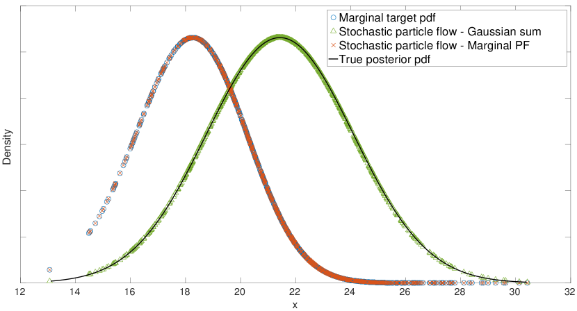
Figure 7.1: Densities generated by the SPF-GS and SPF-MPF for the linear, univariate example

7.1.2 Quadratic, Univariate Model

The quadratic, univariate model was tested with parameters set as shown in the following table. This model is interesting because nonlinearity of the observation process leads to bimodality of the filtered density.

Parameters for the quadratic, univariate model
Initial distribution	$\bar{\mathrm{x}}_{k-1}^{\vphantom{(i)}}=0$, $P_{k-1}=20$
Markov transition pdf	$f(\mathrm{x}_{k-1}^{\vphantom{(i)}})=\mathrm{x}_{k-1}^{\vphantom{(i)}}$, $Q_{k}=20$
Likelihood function	$h(\mathrm{x}_{k}^{\vphantom{(i)}})=\mathrm{x}_{k}^{2}/20$, $R_{k}=50$
Observation	$\mathrm{y}_{k}=30$

This nonlinear example was set to be favourable for marginal importance sampling such that it would be possible to compare different marginal particle filters against the SPF-MPF. The original particle flows, GPF and SDPF, are compared to the SPF-MPF as well. The quantified performances for this quadratic univariate model are shown in Table 1.

Firstly, we compare the sequence of histograms achieved when propagating samples by the GPF, by the SDPF and by the SPF-GS. As it can be seen in Figure 7.2, for this example, stochastic particle flow provides the best distribution of particles to approximate the posterior density, denoting a higher level of accuracy and regularity of the flow formulated as a diffusion.

Regarding the marginal importance densities illustrated in Figure 7.3, we observe a high degree of similarity of the SPF-MPF proposal density to the marginal target density. In the same manner, the filtering density achieved by the SPF-GS accurately approximates the true posterior density, as evidenced in Table 1. In Figure 7.4 we can see in detail the proximity of the SPF-MPF proposal density to both the marginal target density and the true posterior density, along with some of the proposal mixture components. The density proposed by the marginal (optimal) auxiliary particle filter (MAPF) is also very similar to the marginal target, providing an accurate solution, whereas all other filters propose densities less effective for this example. These observations are quantitatively captured by the performance data summarized in Table 1.

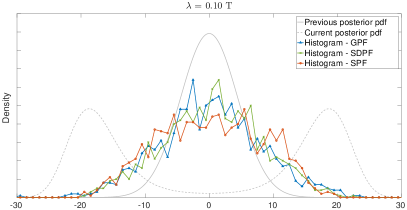
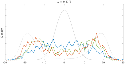
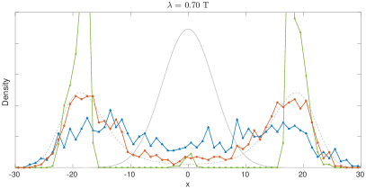
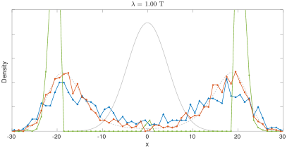
Figure 7.2: Sequence of histograms achieved by propagating particles for the quadratic, univariate example

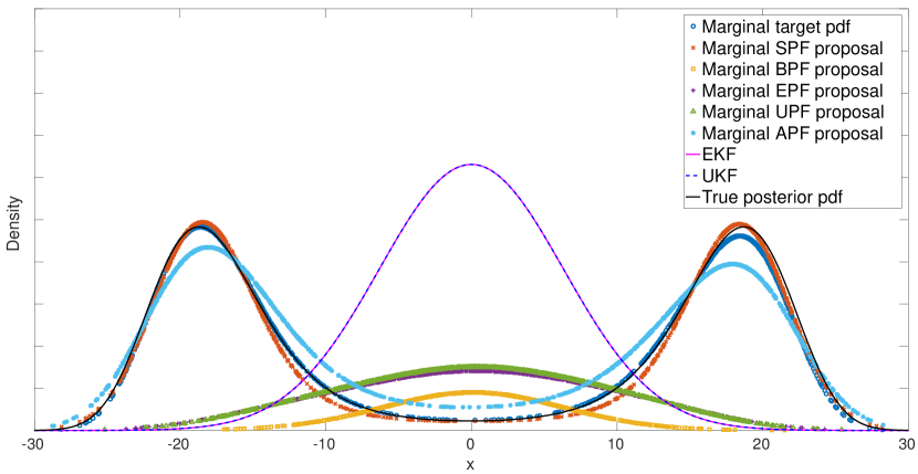
Figure 7.3: Comparison of proposal densities for the quadratic, univariate example

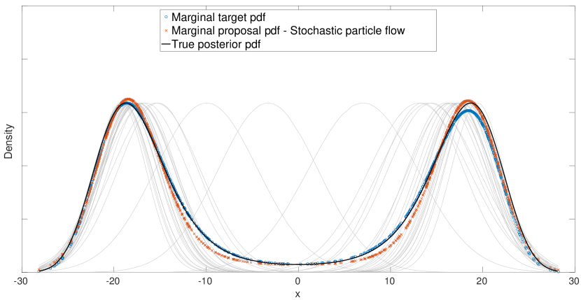
Figure 7.4: Marginal proposal density based on the stochastic particle flow

7.1.3 Cubic, Univariate Model

The cubic, univariate model was tested with parameters set as shown in the following table.

Parameters for the cubic, univariate model
Initial distribution	$\bar{\mathrm{x}}_{k-1}^{\vphantom{(i)}}=0$, $P_{k-1}=20$
Markov transition pdf	$f(\mathrm{x}_{k-1}^{\vphantom{(i)}})=\mathrm{x}_{k-1}^{\vphantom{(i)}}$, $Q_{k}=20$
Likelihood function	$h(\mathrm{x}_{k}^{\vphantom{(i)}})=\mathrm{x}_{k}^{3}/120$, $R_{k}=50$
Observation	$\mathrm{y}_{k}=20$

This nonlinear example was also set to be favourable for marginal importance sampling, i.e., avoiding the scenario described in the first toy example where importance sampling fails. By comparing the resulting histograms achieved when propagating samples by the GPF, by the SDPF and by the stochastic particle flow, it is remarkable in Figure 7.5 that the stochastic particle flow provides a fairly superior distribution of particles to approximate the posterior density. This superiority is incorporated in the importance density proposed by the SPF-MPF as can be seen in Figure 7.6. The importance density proposed by the marginal auxiliary particle filter (MAPF) also provides an accurate solution to the filtering problem, but it is slightly less effective than the SPF-MPF. All the other marginal particle filters present less effective solutions. The comparison of all filters for this example is quantified in Table 1.

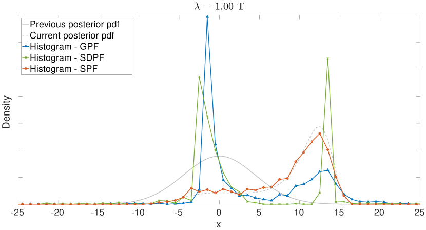
Figure 7.5: Resulting histograms of particles for the cubic, univariate example

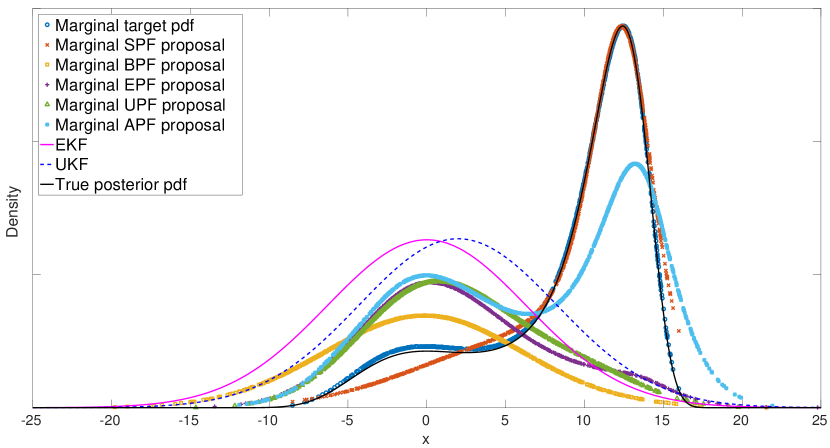
Figure 7.6: Comparison of proposal densities for the cubic, univariate example

Density	Linear				Quadratic				Cubic
	$\text{JSD}_{\text{avg}}$		$\text{ESS}_{\text{avg}}$		$\text{JSD}_{\text{avg}}$		$\text{ESS}_{\text{avg}}$		$\text{JSD}_{\text{avg}}$		$\text{ESS}_{\text{avg}}$
Marginal target	0.	1572	-		0.	0028	-		0.	0001	-
SPF-GS	0.	0000	-		0.	0013	-		0.	0165	-
SPF-MPF	0.	1574	100.	00%	0.	0052	97.	12%	0.	0071	96.	74%
Marginal BPF	0.	9876	0.	21%	0.	2641	1.	79%	0.	1723	12.	60%
Marginal EPF	0.	7857	1.	90%	0.	3097	16.	69%	0.	1820	28.	63%
Marginal UPF	0.	7870	2.	04%	0.	3112	14.	46%	0.	1674	25.	32%
Marginal APF	0.	0670	100.	00%	0.	0153	92.	92%	0.	0596	72.	00%

Table 1: Comparison of densities for the univariate examples

7.1.4 Linear, Bimodal, Bivariate Model

This example poses a bimodal model where the modes arise from two different observations with a joint likelihood explicitly known. In the algorithm for propagating particles, we implemented a scheme that preselects samples to be filtered for either observation. This is done according to a set of indexes that are sampled from a binomial distribution $B\left(u_{1},u_{2};1,w_{l,(1)},w_{l,(2)}\right)\propto w_{l,(1)}^{u_{1}}w_{l,(2)}^{u_{2}}$ where $u_{1},u_{2}\in\left[0,1\right]$, $u_{1}+u_{2}=1$, such that indexes are uniquely associated to either event $u_{1}$ or $u_{2}$, with probability of either observation, $w_{l,(1)}$ or $w_{l,(2)}$ respectively. The linear, bimodal, bivariate model was tested with parameters set as shown in Table 2. These parameters were chosen to result in quite distinct local properties of the two modes.

Parameters for the linear, bimodal, bivariate model
Initial distribution	$\bar{\mathrm{x}}_{k-1}^{\vphantom{(i)}}=\left(\begin{array}[]{c}0\\ 0\end{array}\right)$, $P_{k-1}=\left(\begin{array}[]{cc}9&0\\ 0&9\end{array}\right)_{\vphantom{2}}^{\vphantom{2}}$
Markov transition pdf	$f(\mathrm{x}_{k-1}^{\vphantom{(i)}})=\mathrm{x}_{k-1}^{\vphantom{(i)}}$, $Q_{k}=\left(\begin{array}[]{cc}16&0\\ 0&16\end{array}\right)_{\vphantom{}}^{\vphantom{2}}$
Likelihood function:	$h(\mathrm{x}_{k}^{\vphantom{(i)}})=\mathrm{x}_{k_{\vphantom{2}}}^{\vphantom{3}}$
Mode 1	$R_{k,(1)}=\left(\begin{array}[]{cc}0.8&0\\ 0&0.2\end{array}\right)_{\vphantom{2}}^{\vphantom{2}}$, $w_{l,(1)}=0.2$
Mode 2	$R_{k,(2)}=\left(\begin{array}[]{cc}4.0&0\\ 0&1.0\end{array}\right)_{\vphantom{2}}^{\vphantom{2}}$, $w_{l,(2)}=0.8$
Observations	$\mathrm{y}_{k,(1)}=\left(\begin{array}[]{c}+10\\ +20\end{array}\right)$, $\mathrm{y}_{k,(2)}=\left(\begin{array}[]{c}+10\\ -20\end{array}\right)_{\vphantom{2}}^{\vphantom{2}}$

Table 2: Parameters for the bimodal bivariate model

For this example, we analyze stochastic particle flow methods, SPF-GS and SPF-MPF, against original particle flow methods only. We exemplify the sequence of particles’ distributions acquired by the GPF, by the SDPF and by the stochastic particle flow in Figure 7.7. It becomes clear that the final distribution generated by the stochastic particle flow is closely similar to the true posterior density, precisely describing the local moments of the two modes. In opposition, the GPF generates a distribution that is excessively biased for the most peaky mode whereas the SDPF generates a distribution that does not describe correctly the covariances of each mode.

These findings are quantified by the average Jensen-Shannon divergences presented in Table 5. Table 5 shows a small divergence of the density filtered by the SPF-GS with respect to the true posterior, a small divergence of the SPF-MPF proposal density as well as of the target density, whereas the divergences of the original particle flows are fairly big. The SPF-MPF provides a high effective sample size.

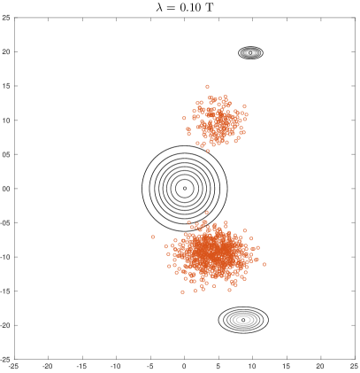
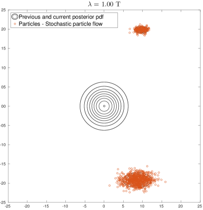
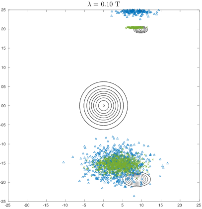
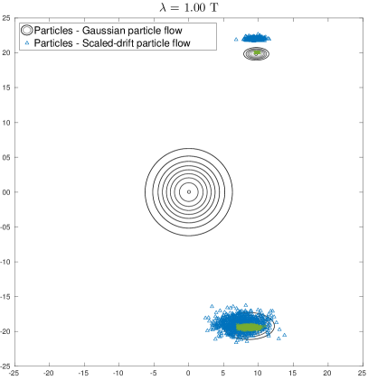
Figure 7.7: Sequence of distributions achieved by propagating particles for the bimodal, bivariate example

7.1.5 Nonlinear, Unimodal, Bivariate Model

The nonlinear bivariate model was tested in two cases:

1. favourable for marginal particle filters, and

2. unfavourable, i.e., emulating a scenario similar to that presented in the first toy example where importance sampling fails.

The parameters used for cases 1 and 2 are presented in Table 3 and Table 4, respectively.

In either cases the sequence of distributions generated by the original particle flows and by the stochastic particle flow are as illustrated in Figure 7.8. Once more it becomes evident that the stochastic particle flow provides a superior distribution of samples to approximate the posterior density, which demonstrates its higher level of accuracy and regularity. Similarly to results presented for previous examples, the GPF seems to generate substantially biased distributions whereas the SDPF seems highly prone to regularity problems. These aspects are well corroborated by the average Jensen-Shannon divergences presented in Table 5.

In the comparison we also included other marginal particle filters. For case 1 (favourable), we illustrate in Figures 7.9 and 7.10 how the marginal importance densities, projected (marginalized) onto the horizontal and vertical planes, would look like as proposed by the marginal auxiliary particle filter (MAPF) and by the SPF-MPF. It is clear that in this case both MAPF and SPF-MPF generate proposal densities quite proximate of the empirical marginal target, which in turn approximates well the true posterior. Additionally, it is possible to visualize that the SPF-MPF provides a slightly better proposal density in terms of similarity to the target density, which is corroborated by a greater average effective sample size as presented in Table 5. All other marginal particle filters don’t generate effective importance densities in terms of approximating either the true posterior or the target density.

For case 2 (unfavourable), importance sampling fails as exemplified by the projections of the importance density proposed by the MAPF depicted in Figure 7.11. By the same reason explained before, the importance sampling procedure fails to provide a satisfactory filtering measure owing to the errors that affect evaluations of both the marginal target density and the marginal importance density. As a consequence, in this case, any marginal particle filter generates a poor solution, although the MAPF provides a high effective sample size. The SPF-MPF generates a remarkably poor solution for case 2 because it distributes particles to approximate the true posterior density by design, but must constrain the proposal mixture components to match a very inaccurate empirical target density.

In contrast, in both cases 1 and 2 the SPF-GS proposes a direct filtering density that accurately approximates the true posterior density. The SPF-GS is demonstrated to be insensitive to the issues caused by an observation located relatively far from the initial distribution. These features are quantitatively captured by the performance indexes summarized in Table 5.

Parameters for the nonlinear bivariate model, case 1
Initial distribution	$\bar{\mathrm{x}}_{k-1}^{\vphantom{(i)}}=\left(\begin{array}[]{c}0\\ 0\end{array}\right)$, $P_{k-1}=\left(\begin{array}[]{cc}20&0\\ 0&20\end{array}\right)_{\vphantom{2}}^{\vphantom{2}}$
Markov transition pdf	$f(\mathrm{x}_{k-1}^{\vphantom{(i)}})=\mathrm{x}_{k-1}^{\vphantom{(i)}}$, $Q_{k}=\left(\begin{array}[]{cc}20&0\\ 0&20\end{array}\right)_{\vphantom{}}^{\vphantom{2}}$
Likelihood function	$h(\mathrm{x}_{k}^{\vphantom{(i)}})=\left(\begin{array}[]{c}\sqrt{\mathrm{x}_{k}\left(1\right)^{2}+\mathrm{x}_{k}\left(2\right)^{2}}\\ \text{atan}\left(\mathrm{x}_{k}\left(2\right)^{\vphantom{2}}/\mathrm{x}_{k}\left(1\right)^{\vphantom{2}}\right)\end{array}\right)_{\vphantom{2}}^{\vphantom{2}}$,
	$R_{k}=\left(\begin{array}[]{cc}1.00&0\\ 0&0.16\end{array}\right)_{\vphantom{2}}^{\vphantom{2}}$
Observation	$\mathrm{y}_{k}=\left(\begin{array}[]{c}20\\ 0^{\circ}\end{array}\right)_{\vphantom{2}}^{\vphantom{2}}$

Table 3: Parameters for the nonlinear bivariate model, case 1

Parameters for the nonlinear bivariate model, case 2
Initial distribution	$\bar{\mathrm{x}}_{k-1}^{\vphantom{(i)}}=\left(\begin{array}[]{c}0\\ 0\end{array}\right)$, $P_{k-1}=\left(\begin{array}[]{cc}10&0\\ 0&10\end{array}\right)_{\vphantom{2}}^{\vphantom{2}}$
Markov transition pdf	$f(\mathrm{x}_{k-1}^{\vphantom{(i)}})=\mathrm{x}_{k-1}^{\vphantom{(i)}}$, $Q_{k}=\left(\begin{array}[]{cc}5&0\\ 0&5\end{array}\right)_{\vphantom{}}^{\vphantom{2}}$
Likelihood function	$h(\mathrm{x}_{k}^{\vphantom{(i)}})=\left(\begin{array}[]{c}\sqrt{\mathrm{x}_{k}\left(1\right)^{2}+\mathrm{x}_{k}\left(2\right)^{2}}\\ \text{atan}\left(\mathrm{x}_{k}\left(2\right)^{\vphantom{2}}/\mathrm{x}_{k}\left(1\right)^{\vphantom{2}}\right)\end{array}\right)_{\vphantom{2}}^{\vphantom{2}}$,
	$R_{k}=\left(\begin{array}[]{cc}1.00&0\\ 0&0.16\end{array}\right)_{\vphantom{2}}^{\vphantom{2}}$
Observation	$\mathrm{y}_{k}=\left(\begin{array}[]{c}20\\ 0^{\circ}\end{array}\right)_{\vphantom{2}}^{\vphantom{2}}$

Table 4: Parameters for the nonlinear bivariate model, case 2

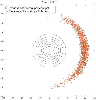
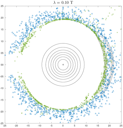
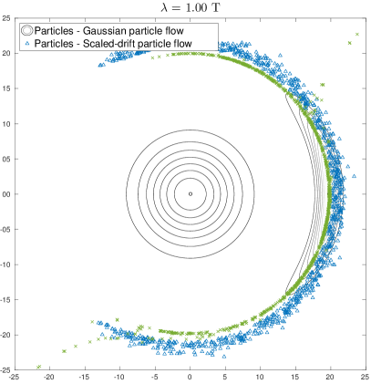
Figure 7.8: Sequence of distributions achieved by propagating particles for the nonlinear, bivariate example

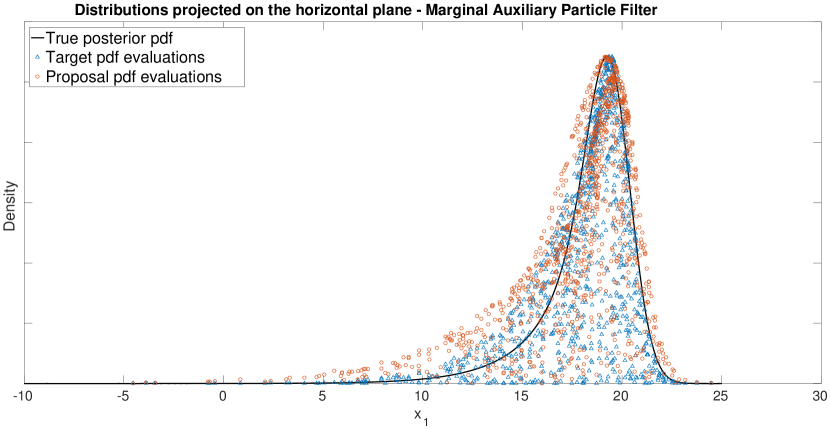
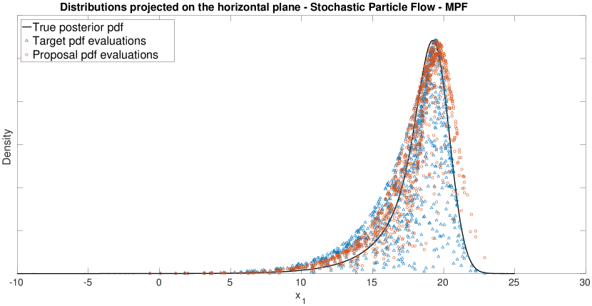
Figure 7.9: Horizontal-plane projection of densities for the MAPF and SPF-MPF (nonlinear, bivariate example)

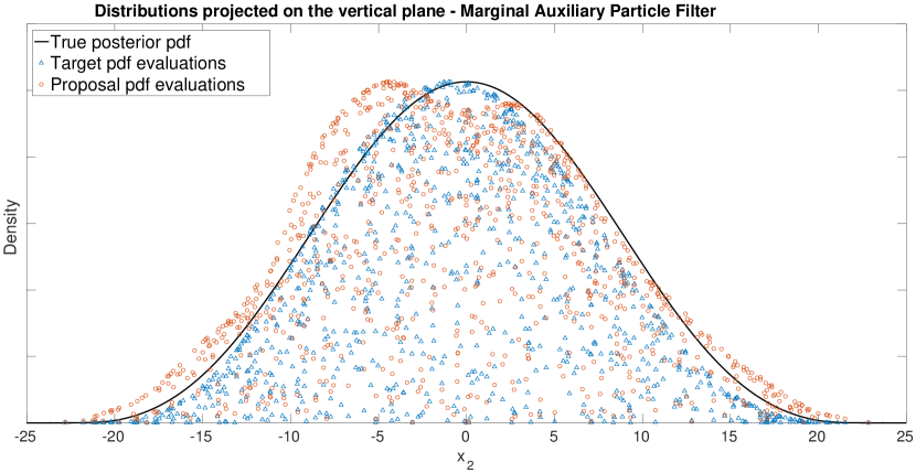
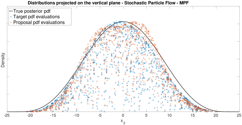
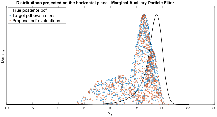
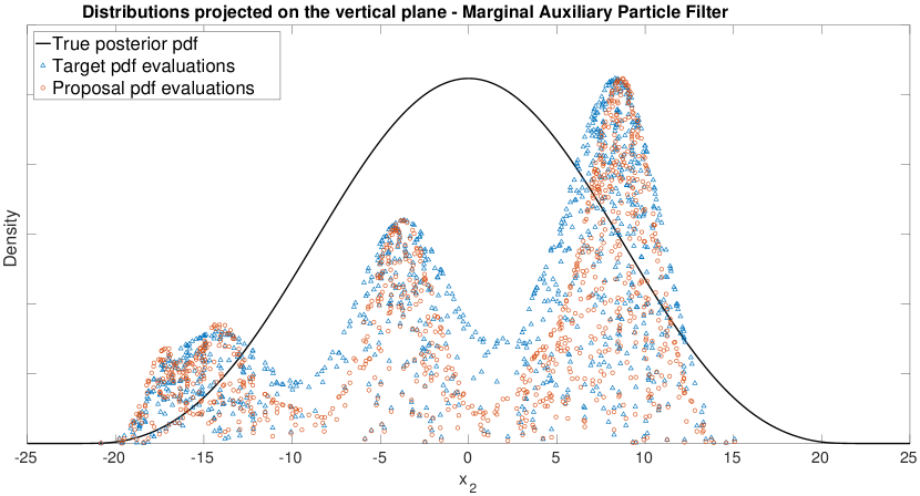
Figure 7.10: Vertical-plane projection of densities for the MAPF and SPF-MPF (nonlinear, bivariate example)

Figure 7.11: Failure of marginal importance sampling for the nonlinear, bivariate example

Density	Multimodal, linear				Nonlinear - case 1				Nonlinear - case 2
	$\text{JSD}_{\text{avg}}$		$\text{ESS}_{\text{avg}}$		$\text{JSD}_{\text{avg}}$		$\text{ESS}_{\text{avg}}$		$\text{JSD}_{\text{avg}}$		$\text{ESS}_{\text{avg}}$
Marginal target	0.	0118	-		0.	0074	-		0.	2444	-
SPF-GS	0.	0003	-		0.	0133	-		0.	0755	-
SPF-MPF	0.	0217	93.	00%	0.	0112	84.	01%	0.	2746	10.	79%
Gaussian particle flow	0.	2647	-		0.	6563	-		0.	5279	-
Scaled-drift particle flow	0.	3866	-		0.	4962	-		0.	5804	-
Marginal BPF	-		-		0.	9969	0.	37%	0.	9998	0.	13%
Marginal EPF	-		-		0.	3131	27.	57%	0.	5714	8.	83%
Marginal UPF	-		-		0.	7753	4.	44%	0.	8136	2.	31%
Marginal APF	-		-		0.	0119	81.	32%	0.	1467	85.	11%

Table 5: Comparison of densities for the bivariate examples

7.2 Multi-Sensor Bearings-Only Tracking

Estimation in clutter of a target’s position and velocity based solely on angular measurements is a relevant problem that finds direct application in airborne radar and sonar in passive listening mode. We propose an example where a single target is observed by a circumferential array of sensors. Each sensor measures the target’s bearing with respect to its own position.

In this example, we compare performances of the following filters:

• multi-sensor EKF that performs a series of centralized measurement updates, considering each sensor in sequence;

• Information Matrix Fusion filter (IMF-EKF) [83] that fuses distributed estimates (in parallel) into a global estimate using the Information Matrix form of the EKF;

• bootstrap particle filter (SIR);

• Gaussian particle flow (GPF);

• scaled-drift particle flow (SDPF); and

• stochastic-particle-flow Gaussian sum (SPF-GS).

As mentioned before, in order to work properly, both the GPF and SDPF are implemented based on a companion filter that estimates the state covariance matrix. This is in accordance with implementations suggested by Choi et al. [50] and Ding & Coates [51]. In this example we used the multi-sensor EKF as companion filter for both the GPF and SDPF. In contrast, the stochastic particle flow does not require a companion filter.

The bootstrap particle filter (SIR), the GPF and SDPF, and the SPF-GS consider all measurements jointly according to a joint likelihood function described in the next section. Performance is analyzed by computing the root-mean-square error (RMSE) of estimates and the normalized-estimation error squared (NEES) over 100 Monte Carlo runs. All particle-based filters use 200 samples.

7.2.1 A Multi-Sensor Bearings-Only Model

When tracking in clutter based on multiple measurements, the usual treatment rests on the probabilistic data association (PDA) [84]. In the PDA model, a set of $m_{k}$ valid measurements is received at each time step $k$ and assumed to be generated according to the possibilities: (i) all measurements are false alarms (clutter), (ii) one of the measurements is originated from the target and the remaining are false alarms. Let $\theta_{k,i}$ be the association event that the $i$th measurement is target-originated. The PDA filter computes the association probabilities $p(\theta_{k,i}|\mathrm{y}_{1:k})$ conditional on the set of all received measurements up to time instant $k$, and calculates the target state posterior density, $p(\mathrm{x}_{k}|\mathrm{y}_{1:k})$, by marginalizing the joint density $p(\mathrm{x}_{k},\theta_{k,1:m_{k}}|\mathrm{y}_{1:k})$ over all possible associations.

In our example a single target is tracked by a set of $N_{s}$ sensors located along a circumference that encloses the surveillance region, at equally-spaced angular positions. As per the PDA model, one target is known to exist a priori, detected with probability $P_{d,j}$ by the $j$th sensor, and the number of clutter detections per sensor is Poisson-distributed with mean $\lambda_{c}\cdot V$, where $\lambda_{c}$ is the clutter spatial density and $V$ is the surveillance region’s volume. For any given set of $N_{s}$ sensors, the expected likelihood can be easily obtained by extending the procedure established by Marrs et al. [85] to multiple sensors, to give

$$p\left(\mathrm{y}_{k}|\mathrm{x}_{k},\mathrm{y}_{1:k-1}\right)=\prod_{j=1}^{N_{s}}V^{-m_{k,j}}\frac{\left(\lambda_{c}V\right)^{m_{k,j}}e^{-\lambda_{c}V}}{m_{k,j}!}\left[\lambda_{c}\left(1-P_{d,j}\right)+\sum_{i=1}^{m_{k,j}}P_{d,j}\mathcal{N}\left(\mathrm{y}_{k,i(j)};h_{j}(\mathrm{x}_{k}),R_{k,j}\right)\right],$$ (7.6)

where $m_{k,j}$ is the total number of validated measurements for the $j$th sensor, $\mathrm{y}_{k,i(j)}$ is the $i$th measurement received by the $j$th sensor, $h_{j}(\cdot)$ and $R_{k,j}$ are the observation function and the observation noise variance for the $j$th sensor, respectively.

On a bidimensional state space, the bearing observations are modeled by

$$h_{j}(\mathrm{x}_{k})=\text{atan}\left(\frac{\mathrm{x}_{k}\left(2\right)-p_{2,j}}{\mathrm{x}_{k}\left(1\right)-p_{1,j}}\right),$$ (7.7)

where $\mathrm{p}_{j}=\left(p_{1,j},p_{2,j}\right)^{T}$ are the position coordinates for the $j$th sensor. We assume a target moving according to the nearly-constant velocity model,

$$\mathrm{x}_{k}^{\vphantom{(i)}}=F\mathrm{x}_{k-1}^{\vphantom{(i)}}+\mathrm{u}_{k},\,\mathrm{u}_{k}\sim\mathcal{N}(\mathrm{u}_{k}^{\vphantom{(i)}};0_{n_{x}},Q_{k}),$$ (7.8)

where $\mathrm{x}_{k}=(p_{x_{1}},p_{x_{2}},v_{x_{1}},v_{x_{2}})_{k}^{T}$ is the state vector composed of position and velocity in Cartesian coordinates $\left(x_{1},x_{2}\right)$, and

$$F_{\hphantom{k}} =\left(\begin{array}[]{cccc}1&0&\Delta t&0\\ 0&1&0&\Delta t\\ 0&0&1&0\\ 0&0&0&1\end{array}\right),$$ (7.13)

$$Q_{k} =\left(\begin{array}[]{cccc}\nicefrac{{\Delta t^{3}}}{{3}}&0&\nicefrac{{\Delta t^{2}}}{{2}}&0\\ 0&\nicefrac{{\Delta t^{3}}}{{3}}&0&\nicefrac{{\Delta t^{2}}}{{2}}\\ \nicefrac{{\Delta t^{2}}}{{2}}&0&\Delta t&0\\ 0&\nicefrac{{\Delta t^{2}}}{{2}}&0&\Delta t\end{array}\right)\sigma_{q}^{2}.$$ (7.18)

The multi-sensor joint likelihood (7.6) is incorporated in the bootstrap (SIR) filter, the GPF and SDPF, and the SPF-GS by considering their filtering densities to target a posterior density involving such joint likelihood. Regarding the implementation of particle flows, specifically for this problem, the GPF and SDPF reinterpret the filtered density empirically as a Gaussian pdf at the end of each iteration in order to avoid exponential growth of the number of mixture components over time. This practical aspect does not affect the SPF-GS, whose filtered density is a mixture composed invariably of $N$ local solutions to the actual posterior pdf, where $N$ is the number of samples (and mixture components).

Generally speaking, multi-sensor bearings-only tracking is a difficult problem to solve when the observation noise has high variance, the probability of detection is relatively low and the probability of having clutter in the surveillance region is not negligible. In this scenario, the difficulty stems from the fact that the joint multi-sensor likelihood (7.6) is a product of mixtures composed of several nonlinear and non-informative likelihood terms: when nonlinearity is pronounced by a high-variance observation noise, the resulting posterior density may not be well expressed by simple parametric densities. In addition, this difficulty is modulated by the amount of information available: the fewer the number of sensors the more difficult to solve the problem. Another aspect that poses additional concern is the system’s observability. It is highly dependent on the relative position of a sensor with respect to the target’s trajectory, i.e., trajectories radially aligned with a sensor’s position provide less information on the target’s velocity.

7.2.2 Results

A challenging scenario was set for comparing the filters in order to exacerbate differences of their performances to a noticeable level. In this very difficult scenario, state process noise is assumed with variance scaled by ${\sigma_{q}^{2}=25\,m^{2}}$, observation noise variance is ${R_{k}=25\,deg^{2}}$, $P_{d}=0.50$ and $\lambda_{c}\times V=1.00$ false alarm/sensor/scan, for identical sensors. Even though estimation errors generated for such a scenario might not be feasible as an Engineering solution, it is certainly of practical interest to examine how the estimates’ errors scale to such extreme scenarios, which might happen in real applications. This problem is particularly interesting because the smaller the number of sensors the more difficult to achieve reasonable estimates since, in this case, the low signal-to-noise ratio would deteriorate inference. For this example, the SPF-GS has been set with time horizon $T=10\,s$ and integration step size $\Delta\lambda=1\,s$.

The resulting track of an exemplar run is shown in Figure 7.12. The track initiation is based on an overdetermined triangulation of measurements for the first two steps. No gating has been performed, i.e., no preprocessing to discard measurements that fall outside a high-confidence region of each sensor. Figure 7.12 depicts a successful tracking of the target despite the difficult scenario.

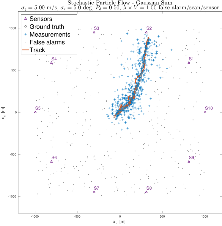
Figure 7.12: Illustration of bearing-only multi-sensor tracking

The resulting root-mean-square error (RMSE), normalized-estimation error squared (NEES), and average computation time (per time step) of all filters for different numbers of sensors are shown in Figures 7.13, 7.14 and 7.15 respectively. The following important aspects can be observed from Figure 7.13:

• Somewhat counterintuitively, the multi-sensor serial EKF provides better estimates than that of Information Matrix Fusion EKF (IMF-EKF), both in terms of precision (RMSE) and “consistency” (or credibility as indicated by NEES).

• The scaled-drift particle flow (SDPF) shows remarkably poor performance.

• The bootstrap particle filter (SIR) provides mediocre performance, eventually becoming better than the IMF-EKF as the number of sensors increases.

• Accuracies shown by the Gaussian particle flow (GPF) and the serial EKF are commensurate and similar to that of stochastic particle flow (SPF-GS) when the number of sensors is high.

• As expected, the overall estimation accuracy is improved as the number of sensors is increased.

• The SPF-GS provides the most accurate estimates in difficult scenarios, i.e., when the number of sensors is small.

• Estimation by the SPF-GS is more consistent (or credible), which is denoted by an NEES closer to one ($\log_{10}NEES\rightarrow 0$) from above.

It is worth commenting on the results comparing GPF and SPF-GS. Specifically for this problem, when the number of sensors is sufficiently high, the GPF provides estimates as accurate as those of SPF-GS at a slightly lower computational cost. It is also remakable the successful synergy between the GPF and its companion filter, a multi-sensor serial EKF that provides the covariance estimates. However, it is difficult to justify the calculated NEES for original particle flows since their first and second moment estimates are underpinned by distinct filtering methods. On the other hand, stochastic particle flow (SPF-GS) provides fairly accurate state estimates and securely constitutes the most credible estimator among all evaluated filters.

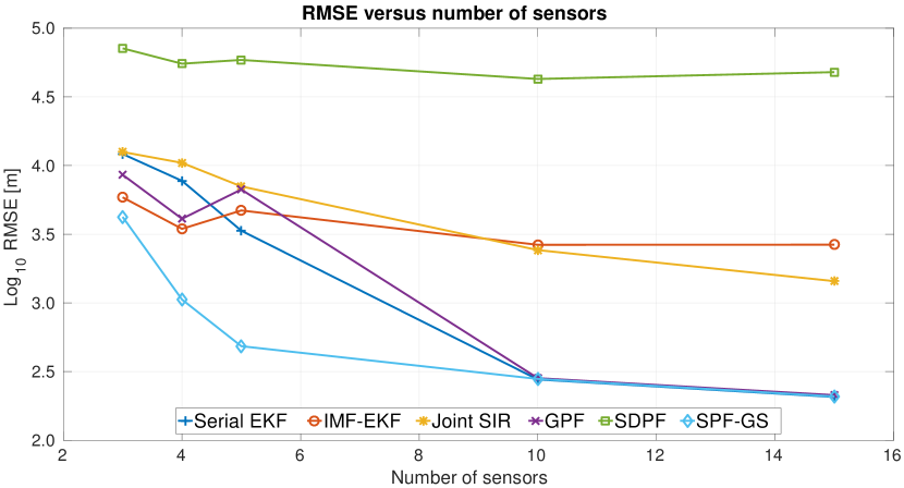
Figure 7.13: RMSE for the multi-sensor bearing-only tracking example

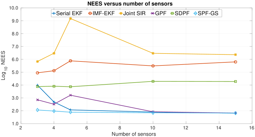
Figure 7.14: NEES for the multi-sensor bearing-only tracking example

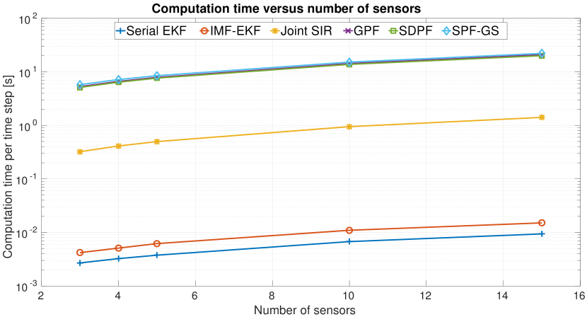
Figure 7.15: Average computation time for the multi-sensor bearing-only tracking example

7.3 Convoy Tracking

Tracking multiple objects in clutter is as challenging as important for real applications. In the multi-target tracking standard methods, the most common treatment assumes the targets’ states to be independent so that the joint probability density is the product of their marginal densities. While this assumption is fairly reasonable for applications where objects are far apart most of the time, the same cannot be stated for cases where objects are in proximity for a considerable part of time. This latter cases elicit tracking all targets jointly in the hope of implicitly capturing dependencies between targets. When targets are tracked jointly the problem’s dimensionality scales with the number of targets.

To illustrate this situation, we propose an example of a convoy of vehicles that are forced into mutual proximity when trafficking on a road . The vehicles have explicit interactions as each driver aims driving at the maximum allowed speed unless there is another vehicle immediately in front at a slower speed. This scenario demands care for a safety distance. The intent of the tracker is then to provide the best estimate of each vehicle on a convoy, given a set of non-identified measurements corrupted by noise and possible false alarms (clutter) reported by a position sensor.

We compare performances of the following filters:

• Joint Probabilistic Data Association (JPDA) filter [84];

• Global Nearest Neighbor Data Association (GNN) filter;

• JPDA with a Gaussian mixture per target (JPDA-GM), applying mixture reduction [87];

• Coupled Probabilistic Data Association (CPDA) filter [88];

• multi-target bootstrap particle filter (joint SIR) based on the description by Blom & Bloem [89];

• Gaussian particle flow (GPF);

• scaled-drift particle flow (SDPF); and

• stochastic-particle-flow Gaussian sum (SPF-GS).

The GPF and the SDPF rely on a companion filter to estimate state covariance matrices correctly, according to implementation guidelines by Choi et al. [50] and Ding & Coates [51]. In this example, we used the CPDA [88] as companion filter for the original particle flows (GPF, SDPF). In contrast, the SPF-GS does not require a companion filter.

The CPDA, the joint bootstrap particle filter (SIR), the GPF and SDPF, and the SPF-GS consider all targets’ states jointly, as a single high-dimensional state. In contrast, the classical multi-target filters track targets separately, where each target’s state is described by the nearly-constant velocity model. Performance is analyzed by computing the root-mean-square error (RMSE) of estimates and the normalized-estimation error squared (NEES) over 100 Monte Carlo runs. The particle filter (SIR), the original particle flows and stochastic particle flow use 200 samples.

7.3.1 The Intelligent Driver Model

The Intelligent Driver Model (IDM) [90] is a model used in Traffic Engineering to simulate phenomena such as congestion and to analyze the traffic behaviour as a response to changes in the transport system. Because the interaction between vehicles is explicitly taken into account by the IDM, tracking based on it involves consideration of the joint state of multiple targets. Even though the IDM establishes an empirical description of traffic for multiple vehicles, it has not been previously used in the context of multi-target tracking. We propose a stochastic version of the IDM and discretize it in order to make it compatible with multi-target trackers formulated on the joint state space.

The IDM describes the dynamics of vehicles in traffic, in terms of positions and velocities, incorporating the interaction between each vehicle and the vehicle directly in front. Provided a vehicle indexed as $\alpha$ with length $l_{\alpha}$, the dynamics of its position $x_{\alpha}$ and velocity $v_{\alpha}$ are given by the following (continuous-time) stochastic differential equations:

$$dx_{\alpha} =v_{\alpha}dt,$$ (7.19)

$$dv_{\alpha} =\underbrace{a\left[1-\left(\frac{v_{\alpha}}{v_{0}}\right)^{\delta}\right]^{\vphantom{2}}}_{\dot{v}_{\alpha}^{\text{free road$\hphantom{o}$}}}dt-\underbrace{a\left[\frac{\bar{s}}{s_{\alpha}}\vphantom{\left(\frac{v_{\alpha}}{v_{0}}\right)^{\delta}}\right]^{2}}_{\dot{v}_{\alpha}^{\text{interaction}}}dt+dw_{t},$$ (7.20)

where $\left\{w_{t}\right\}_{t\geq 0}$ is a Wiener process, ${s_{\alpha}=x_{\alpha-1}-x_{\alpha}-l_{\alpha}}$ is the net distance between vehicles, the approaching rate is given by ${\Delta v_{\alpha}=v_{\alpha-1}-v_{\alpha}}$, and ${\bar{s}=\bar{s}\left(v_{\alpha},\Delta v_{\alpha}\right)}$ is the expected distance defined as

$$\bar{s}\left(v_{\alpha},\Delta v_{\alpha}\right)=s_{0}+v_{\alpha}T_{h}+\frac{v_{\alpha}\Delta v_{\alpha}}{2\sqrt{a\cdot b}}.$$ (7.21)

The model dynamics is such that when a vehicle is travelling on a free road it will predominantly accelerate according to $\dot{v}_{\alpha}^{\text{free road}}$ up to the maximum allowed speed $v_{0}$, whereas when it approaches another vehicle immediately in front, the decrement in acceleration according to $\dot{v}_{\alpha}^{\text{interaction}}$ becomes relevant to maintain a safe-time headway $T_{h}$ and to avoid approaching closer than the minimum safe distance $s_{0}$. The IDM parameters are summarized in the following table.

Parameter	Description
$a$	nominal maximum acceleration
$b$	comfortable braking decceleration
$\delta$	acceleration exponent (driver dynamics)
$v_{0}$	free-road desired velocity
$s_{0}$	minimum allowed distance between vehicles
$T_{h}$	safe-time headway
$\alpha-1$	index of the vehicle direcly in front

In order to use the stochastic IDM as the state process for a multi-target tracker, its continuous-time equations are discretized by a first-order approximation (Markov random field). This assumes that the state’s derivative with respect to time is linear in time between two subsequent measurements, but the interactions between non-adjacent vehicles are negligible when compared to the interactions between adjacent vehicles. The discretized version of the stochastic IDM is presented in the Appendix D.

7.3.2 The Multi-Target Joint Likelihood Function

The joint multi-target filters extend the joint probabilistic data association (JPDA) [84] framework for situations where the targets’ states are not mutually independent conditioned on the past observations. This formulation has been first proposed as the JPDA Coupled filter (JPDAC) [84] and further generalized by Blom & Bloem [88, 89] who consider the measurement-to-target associations implicitly.

In the JPDA model, a set of $N_{m}$ valid measurements is received at each time step $k$ and assumed to be generated according to the possibilities: (i) each of the measurements may be originated from each target, considering all possible associations, (ii) a measurement not originated from any target is due to a false alarm (clutter). These possibilities are exhaustive such that a measurement can have only one source, and at most one of the validated measurements can originate from a target.

Let ${\phi_{k,i}\in\left\{0,1,\,\dots,\,N_{m}\right\}}$ be an association event that maps each target $i\in\{1,\dots,N_{t}\}$ to the measurement indexed as $\phi_{k,i}$, where $\phi_{k,i}=0$ means that no measurement is associated to the $i$th target. The Coupled JPDA filter computes the joint association probabilities $p(\phi_{k,1:N_{t}}|\mathrm{y}_{1:k})$ conditional on the set of all received measurements up to time instant $k$, and calculates the joint state posterior density, $p(\mathrm{x}_{k,1:N_{t}}|\mathrm{y}_{1:k})$, by marginalizing $p(\mathrm{x}_{k,1:N_{t}},\phi_{k,1:N_{t}}|\mathrm{y}_{1:k})$ over all possible joint associations.

In the JPDA framework, $N_{t}$ targets are known to exist a priori, detected with probability $P_{d}$ by a single sensor; the number of clutter detections is Poisson-distributed with mean $\lambda_{c}\cdot V$, where $\lambda_{c}$ is the clutter spatial density and $V$ is the surveillance region’s volume; the location of each clutter detection is independently distributed according to a spatial density $\eta_{c}(\mathrm{y})$; and the likelihood function of the $j$th measurement being originated from the $i$th detected target is $p(\mathrm{y}_{k,j}|\mathrm{x}_{k,i})$. Denoting the joint multi-target state as $\mathrm{x}_{k,1:N_{t}}$ and the joint observation as $\mathrm{y}_{k,1:N_{m}},$ the joint likelihood can be either obtained as in [89] or by a formulation equivalent to the Coupled JPDA as

$$p\left(\mathrm{y}_{k,1:N_{m}}|\mathrm{x}_{k,1:N_{t}}\right)\\ =\frac{\left[\prod_{j=1}^{N_{m}}\eta_{c}\left(\mathrm{y}_{k,j}\right)\right]}{N_{t}!}\sum_{N_{d}=0}^{N_{t}}\frac{\left(\lambda_{c}V\right)^{N_{m}-N_{d}}e^{-\lambda_{c}V}}{\left(N_{m}-N_{d}\right)!}P_{d}^{N_{d}}\left(1-P_{d}\right)^{N_{t}-N_{d}}\sum_{\phi_{k,1:N_{t}}|N_{d}}\prod_{i=1}^{N_{t}}\frac{p\left(\mathrm{y}_{k,\phi_{k,i}}|\mathrm{x}_{k,i}\right)}{\eta_{c}\left(\mathrm{y}_{k,\phi_{k,i}}\right)}.$$ (7.22)

The joint state vector $\mathrm{x}_{k,1:N_{t}}=(p_{1},\dots,p_{N_{t}},v_{1},\dots,v_{N_{t}})_{k}^{T}$ is composed of position and velocity of all vehicles in the convoy, and the joint observation $\mathrm{y}_{k,1:N_{m}}=(\mathrm{y_{1},\dots,\mathrm{y}}_{N_{m}})_{k}^{T}$ contains position measurements of all targets and possible false alarms obtained at a given time instant $k$.

The joint bootstrap particle filter, the GPF and SDPF, and the SPF-GS consider their filtering densities to target a joint posterior density incorporating the joint multi-target likelihood function (7.22). Regarding the implementation of original particle flows, the GPF and SDPF reinterpret the filtered density empirically as a Gaussian pdf at the end of each iteration in order to avoid exponential growth of the number of mixture components over time. In contrast, this practical aspect does not affect the stochastic particle flow, whose filtered density is a mixture composed of a fixed number of local solutions to the actual posterior pdf.

7.3.3 Results

We simulated the trajectories of vehicles on a ring road by integrating the continuous-time stochastic IDM over 60 seconds with the parameters presented as follows. The convoy was set to start from rest with the vehicles initially positioned apart, led by a truck so that the queue of cars is slowed down and forced into mutual proximity. The minimum allowed distance between vehicles was set to be exaggeratedly small ($s_{0}=0.5\,m$) to induce the model to control the distance between cars mainly based on the safe-time headway $T_{h}$. In this case, the safe-time headway indirectly determines the desired distance between vehicles, which is denoted as target distance in the table below. At the final steady state, the net speed of the convoy is dominated by the free-road speed of the truck, which motivates the safe-time headway being computed based on $v_{0,\text{truck}}$.

Parameter	car	truck
$a$	$0.5\,m/s^{2}$	$0.4\,m/s^{2}$
$b$	$1.5\,m/s^{2}$	$1.2\,m/s^{2}$
$\delta$	$4$	$4$
$v_{0}$	$15\,m/s$	$10\,m/s$
$s_{0}$	$0.5\,m$	$0.5\,m$
$T_{h}$	$\frac{\vphantom{()^{2}}\text{\{\text{target distance (m)}\}}}{v_{0,\text{truck}}}$	-
$l_{\alpha}$	$5\,m$	$20\,m$

The joint state process covariance matrix is assumed as scaled by ${\sigma_{q}^{2}=0.0625\,\left(m/s\right)^{2}}$, each position observation has variance ${\sigma_{r}^{2}=4\,m^{2}}$, ${P_{d}=0.80}$ and $\lambda_{c}\times V=0.01$ false alarm/scan, and the surveillance region’s “volume”, $V$, is in fact the length covered by a confidence region ($\approx 99.73\%$) that contains all the vehicles. Proposing a method to effectively initiate tracks was out of the example’s scope, thus track initiation was considered to be ideal, i.e., the initial position and velocity of the targets are known with initial uncertainty scaled by the observation noise. The stochastic particle flow has been set with time horizon $T=15\,s$ and integration step size $\Delta\lambda=1\,s$.

Figure 7.20 shows two frames of an exemplar run, demonstrating the situation where a queue of cars is slowed down by a truck, forcing them into proximity. The non-filled rectangles depicted in Figure 7.20 denote the position estimates provided by the filter applied for that run. Interactions between vehicles in the convoy, due to proximity, can be well perceived by position estimates of the exemplar run as shown in Figure 7.19.

The resulting root-mean-square error (RMSE), normalized-estimation error squared (NEES), and average computation time (per time step) of all filters, for different numbers of vehicles, and target distance between vehicles $d=10\,m$, are shown in Figures 7.16, 7.17 and 7.18 respectively. RMSE and NEES were computed over 100 Monte Carlo runs, with the particle-based filters using 200 samples. The following important aspects can be noted from Figure 7.16:

• In general, trackers that estimate on the joint $2N_{t}$-dimensional state space clearly outperform the classical multi-target trackers (JPDA, GNN and JPDA-GM), both in terms of precision (RMSE) and credibility (NEES).

• Among the classical multi-target trackers, the Global Nearest Neighbor (GNN) association filter is the one that provides the most accurate estimates. This can be explained by an increasingly detrimental effect of the association uncertainty on estimation, which is more prominent in the JPDA and less prominent on the GNN filter.

• Estimation errors committed by the multi-target particle filter (joint SIR) grow exponentially with the number of state-space dimensions ($2N_{t}$), as expected, due to the curse of dimensionality.

• The Coupled PDA (CPDA) and the SPF-GS present commensurate root-mean-square errors, suggesting that most of their accuracy gain originates from tracking on the joint $2N_{t}$-dimensional state space and accounting for inherent dependencies between targets.

• The original particle flows (GPF, SDPF) show significant values of NEES. Most likely this is because the evaluated implementation of these filters cannot provide reliable estimates for state covariance matrices and depend on a dissimilar companion filter to work around it, which affects consistency of their estimates.

• The SPF-GS provides overall higher estimation accuracy (RMSE) and consistency (NEES), with low sensitivity to increasing the problem’s number of dimensions.

Based on the results for this example, two important remarks are worth making. Firstly, the results show a notable performance improvement with adoption of filtering on the joint $2N_{t}$-dimensional state space: about 30-fold improvement in estimation precision (RMSE) and nearly 10-fold in credibility (NEES). The fact that the Coupled PDA performs as well as the SPF-GS suggests that modeling inherent dependencies between targets and filtering on the joint space provides most of the performance gain. Secondly, the example not only illustrates well the curse of dimensionality for the multi-target particle filter (joint SIR), but also corroborates the success of principled choices made in the SPF’s formulation in order to avoid degeneracy in high-dimensional problems. This latter observation becomes clear when we realize that the performance indexes for stochastic particle flow scale gently with the number of dimensions.

Additionally, it is also worth noting that the original particle flows provide relatively accurate estimates, scaling well with the number of dimensions. For the evaluated implementation, both particle flow filters (GPF, SDPF) rely on covariance matrices estimated by the CPDA as a companion filter. Due to this fact, calculated NEES for these filters is not reliable since their first and second moment estimates are underpinned by distinct filtering methods. This does not disqualify the original particle filters per se since observed characteristics are probably due to the implementation settings. Under these circumstances, actual consistency (credibility) of their estimates cannot be quantified and, ultimately, evokes the question about the extent to which the success of the adopted implementation is due to the companion filter.

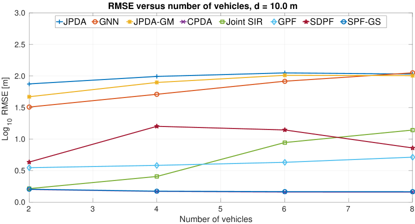
Figure 7.16: RMSE for the convoy tracking example

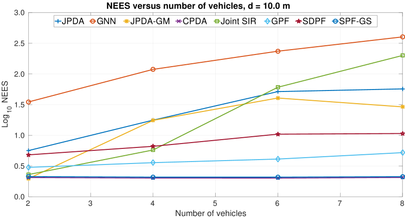
Figure 7.17: NEES for the convoy tracking example

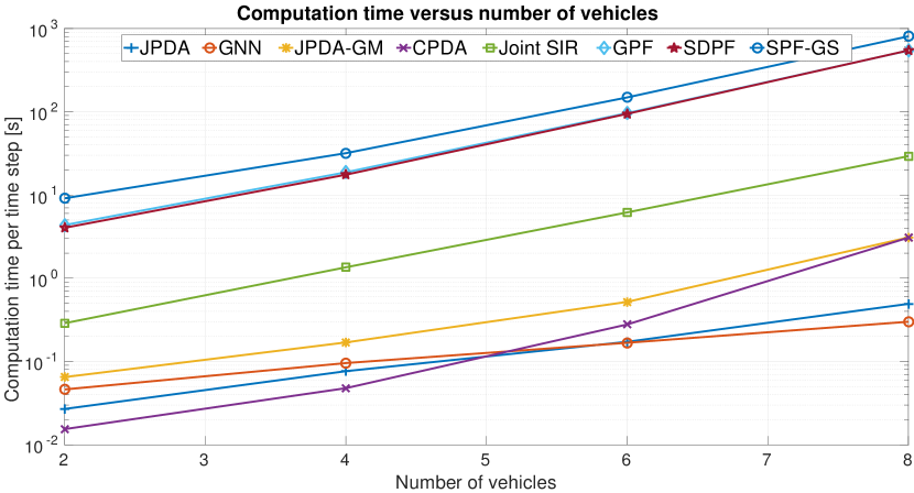
Figure 7.18: Average computation time for the convoy tracking example

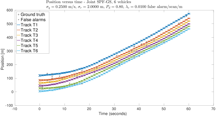
Figure 7.19: Position estimates for an exemplar run of the convoy tracking

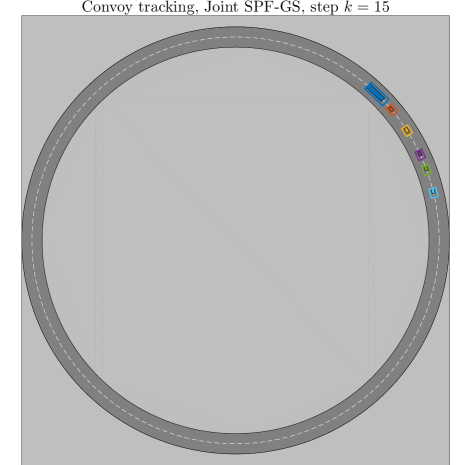
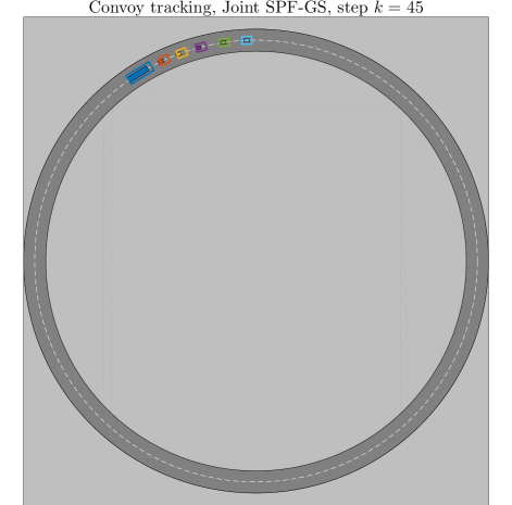
Figure 7.20: Illustration of convoy tracking on a ring road

7.4 Inference on Large Spatial Sensor Networks

In this section we consider the problem proposed by Septier & Peters [56], posed to address inference of physical quantities of complex phenomena from a collection of noisy measurements obtained by a large network of spatially distributed sensors. According to Septier & Peters [56], a large number of applications could adopt such sensor networks to make inferences related to complex phenomena. Applications include environmental monitoring, weather forecasting etc. In this framework, a fusion center would regularly receive observations from sensors set up as a grid, which monitor a time-varying physical phenomenon presenting spatially diverse attributes such as pressure, temperature, concentrations of substance, radiation levels, seismic activity etc. Upon fusing the observations, the solution to the problem consists of estimating the phenomenon state at the current time instant at each of the sensor’s positions. The problem becomes particularly challenging as the number of sensors in the grid increases, since solving the problem then demands efficient algorithms for inference in high-dimensions.

The physical phenomenon is modeled as a time-varying spatially-dependent continuous process defined over a two-dimensional space which is observed sequentially in time by a 2D spatial grid of $n_{x}=N_{s}$ sensors, where $n_{x}$ is the state dimension. At time instant $k$, each sensor independently produces a noisy measurement of an attribute of interest about the phenomenon at its specific location, giving $\mathrm{y}_{k,j}|\mathrm{x}_{k}\sim p(\mathrm{y}_{k}^{(j)}|\mathrm{x}_{k}^{\vphantom{(j)}}),\,\forall j=1,\dots,N_{s}$. Based on the historic set of observations $\mathrm{Y}_{1:k}\coloneqq\{\mathrm{Y}_{k^{\prime}}:k^{\prime}=1,\dots,k\}$, where $Y_{k}\coloneqq\{\mathrm{y}_{k,j}:j=1,\dots,N_{s}\}$, one is required to estimate, at time $k$, the state of the physical phenomenon $\mathrm{x}_{k}\in\mathbb{R}^{n_{x}}$ across the locations of all sensors in the grid. The state process that models the time-varying physical phenomenon is considered to follow a transition multivariate Generalized Hyperbolic (GH) density as

$$p_{t}\left(\mathrm{x}_{k}|\mathrm{x}_{k-1}\right)\propto\frac{\mathbb{K}_{c_{1}-\nicefrac{{n_{x}}}{{2}}}\left[\sqrt{(c_{2}+Q(\mathrm{x}_{k},\mathrm{x}_{k-1}))(c_{3}+\mathrm{\gamma}^{T}\Sigma^{-1}\mathrm{\gamma})}\right]}{\left(\sqrt{(c_{2}+Q(\mathrm{x}_{k},\mathrm{x}_{k-1}))(c_{3}+\mathrm{\gamma}^{T}\Sigma^{-1}\mathrm{\gamma})}\right)^{\nicefrac{{n_{x}}}{{2}}-c_{1}}}\cdot e^{(\mathrm{x}_{k}-\alpha\mathrm{x}_{k-1})\Sigma^{-1}\mathrm{\gamma}}$$ (7.23)

where $Q(\mathrm{x}_{k},\mathrm{x}_{k-1})=(\mathrm{x}_{k}-\alpha\mathrm{x}_{k-1})^{T}\Sigma^{-1}(\mathrm{x}_{k}-\alpha\mathrm{x}_{k-1})$, $\alpha\in\mathbb{R}$ is the location constant, and $\mathbb{K}_{c_{1}}[\cdot]$ denotes the modified Bessel function of the second kind, of order $c_{1}$. The parameters $c_{1}$, $c_{2}$, and $c_{3}$ are scalar values that determine the shape of the distribution, $\Sigma\in\mathbb{R}^{n_{x}\times n_{x}}$ is the dispersion matrix, and the vector $\mathrm{\gamma}\in\mathbb{R}^{n_{x}}$ is the skewness parameter. The choice of transition density in 7.23 can account for heavy-tailed and asymmetric data [56], which is beneficial when modeling physical process with extremal behavior. In special cases, the transition density becomes the normal, normal inverse Gaussian, skewed-t, and other densities. To generate the prior distribution at the first time step, we take $p_{x}(\mathrm{x}_{0})=p_{t}(\mathrm{x}_{0}|\mathrm{x}_{-1}=0)$.

The dispersion matrix is positive definite and is defined such that the degree of spatial correlation across sites of a physical phenomenon is given in terms of the separation between locations as

$$\left[\Sigma\right]_{ij}=\alpha_{0}\exp\left[-\beta^{-1}\|\mathcal{S}_{i}-\mathcal{S}_{j}\|_{2}^{2}\right]+\alpha_{1}\delta_{ij},$$ (7.24)

where $\|\cdot\|_{2}$ is the L2-norm, $\delta_{ij}$ the Kronecker symbol, $\alpha_{0},\alpha_{1}\in\mathbb{R}$, and $\mathcal{S}_{m}\in\mathbb{R}^{2}$ are the physical locations of the sensors for $m=1,\dots,N_{s}$.

For this example, we compare the performance of following filters:

• the Sequential Importance Resampling filter (SIR);

• the block SIR filter, which partitions the state space into separate subspaces of smaller dimensions (blocks of 4 sensors each) and run a particle filter on each subspace [23];

• the Sequential manifold Metropolis-Adjusted Algorithm (SmMALA) filter [10, 56];

• the Sequential manifold Hamiltonian Monte Carlo (SmHMC) filter [10, 56];

• the Stochastic Particle Flow, Gaussian sum (SPF-GS).

These filters are compared for two cases:

• Gaussian state process and Gaussian likelihood;

• Skewed-t state process and Poisson-distributed observations.

Note that SmMALA and SmHMC are chosen because we perceive they constitute two of the best sequential MCMC filters that exist. It is essential to justify why we have not included annealed importance sampling (AIS) [4] and SMC samplers [5] in our comparisons. Although these techniques are built on fast mixing Markov chains, their filtering procedures operate on the joint space along the complete path of samples. This makes them highly prone to the curse of dimensionality for long-time horizons. A careful explanation of this issue can be found in [80] (and Section 6.1), but the key point is that as dimension increases, it becomes increasingly important to avoid consideration of the path. SMC samplers could be adapted to filter in the marginal space (at the cost of up to $\mathcal{O}(N^{3})$ evaluations) but this would require an ad-hoc approximation to the target pdf. Developing the approximations that would be needed to enable SMC samplers to be applied to the problem we consider is not the focus of our paper. We have compared performance of SPF-GS with state-of-the-art techniques (SmMALA and SmHMC) that consider the marginal distribution as well as techniques (SIR and block SIR) that we perceive to be good examples of the class of algorithms, which also includes AIS and SMC samplers, that consider the joint space of the complete sample path and can be applied, without modifications, to the problem we are focused on solving.

These filters are compared for two cases:

• Gaussian state process and Gaussian likelihood;

• Skewed-t state process and Poisson-distributed observations.

The implementations of SmMALA and SmHMC used are exactly as made available by Septier & Peters [56] on their web page. These algorithms make use of a refinement step of the state [56] at the current time, performed with a random partitioning of size 4, by using the empirical approximation of the previous posterior distribution as proposal distribution.

7.4.1 Results

Gaussian State Process and Gaussian Likelihood

We first consider a trivial special case of the GH family as the transition density, namely the multivariate normal distribution. In this setting, each sensor measures the attribute of a physical process with some Gaussian noise. The resulting model is given by

$$p_{t}(\mathrm{x}_{k}|\mathrm{x}_{k-1}) =\mathcal{N}(\mathrm{x}_{k};\,\alpha\mathrm{x}_{k-1},\Sigma),$$

$$p(\mathrm{y}_{k}|\mathrm{x}_{k}) =\mathcal{N}(\mathrm{y}_{k};\,\hphantom{\alpha}\mathrm{x}_{k},_{\hphantom{-1}}R),$$ (7.25)

where $R=\sigma_{y}^{2}\mathbb{I}_{n_{x}}$, and the following model parameters are used: $\alpha=0.9$, $\sigma_{y}^{2}=2$, and with the dispersion matrix constructed using $\alpha_{0}=3$, $\alpha_{1}=0.01$, $\beta=20$. When performing the comparison between the filters, we use as a reference the estimates provided by the Kalman filter (which is optimal in this special case). For the SmMALA and SmHMC, the proposed metric tensor is given by $G\left(\mathrm{x}_{k}\right)=R^{-1}+\Sigma^{-1}$.

The methodology presented in [56] for performance evaluation was reproduced. Instead of presenting the baseline (provided by the Kalman filter) performance explicitly, the accuracy of each filter is evaluated with respect to the baseline performance, i.e., we observe the difference between the log mean square error for each filter against the log mean square error for the Kalman filter. The relative log mean square error, log normalized-estimation error squared (NEES) and average computation time (per time step) of all filters, for different numbers of sensors in the grid, are shown in Figures 7.21, 7.22, 7.23 respectively. The mean square error of the estimates were computed over 100 Monte Carlo runs, with the particle-based filters using 200 samples. The step size adopted for the sequential MCMC filters is $\Delta\lambda=0.5$ and the number of steps obtained as $L=L_{0}+N$, where $L_{0}=0.2N$ is the number of steps for the burn-in phase, whereas for the SPF-GS we applied the empirical rules for time horizon and step step size as presented in subsection 4.6. From Figures 7.21, 7.22, 7.23, we can note that for this example:

• The performances of all sequential MCMC filters are in accordance with the results shown in [56].

• The SPF-GS outperforms all other filters in terms of mean square error and normalized-estimation error squared.

• The SPF-GS demands the highest computational effort when the number of sensors is small, and its computing time scales better than that of SmMALA and worse than that of SmHMC for higher dimensions.

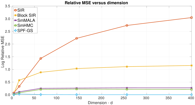
Figure 7.21: Relative MSE for the linear, Gaussian sensor network example

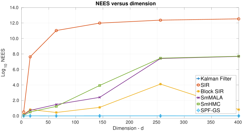
Figure 7.22: NEES for the linear, Gaussian sensor network example

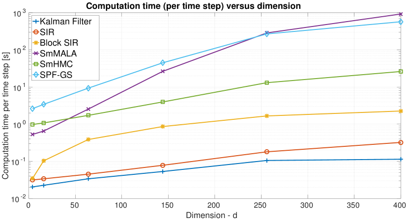
Figure 7.23: Average computation time for the linear, Gaussian sensor network example

The results suggest that SPF-GS is the most accurate among the compared methods. It is unambiguous that the consistency of the estimates produced by the SPF-GS is better than that by all other filters: the NEES for SPF-GS is very close to one (from above) for all evaluated dimensions. It may be well possible that better results could be achieved for the sequential MCMC filters by carefully choosing the step size and number of steps. This would slightly change the performance indexes. However, we strongly believe that such changes would not be enough to modify the conclusions. Additional tests with the SPF-GS demonstrate the computational cost can be directly traded with estimation accuracy. By allowing more steps, via the criteria of Section 4.6, SPF-GS is very close to optimal as depicted in Figure 7.21. On the other hand, if one fixes the step size to $\Delta\lambda=0.5$ and number of steps to $L=20$, the results are as presented in Figures 7.21 and 7.23, where it is becomes clear computational cost alleviation at the expense of slightly degrading mean square error.

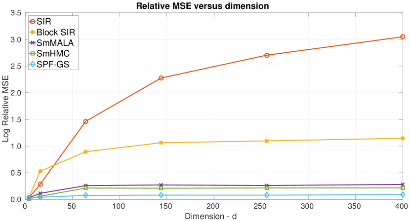
Figure 7.24: Relative MSE for the linear, Gaussian example (SPF-GS with $\Delta\lambda=0.5$, $L=20$)

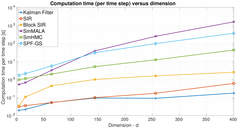
Figure 7.25: Computation time for the linear, Gaussian example (SPF-GS with $\Delta\lambda=0.5$, $L=20$)

Skewed-t State Process with Poisson-Distributed Observations

A high-dimensional non-linear and non-Gaussian state-space model is now studied. The transition kernel is proposed to be a multivariate GH skewed-t density described by (7.23) with $c_{1}=-\nu/2$, $c_{2}=\nu$ and $c_{3}=0$. The likelihood function is assumed to be a Poisson distribution, highly non-linear on the state $\mathrm{x}_{k}$, given by

$$p(\mathrm{y}_{k}|\mathrm{x}_{k})=\prod_{j=1}^{n_{x}}\frac{\lambda_{j}(\mathrm{x}_{j,k})^{\mathrm{y}_{j,k}}}{\mathrm{y}_{j,k}!}e^{-\lambda_{j}(\mathrm{x}_{j,k})},\quad\lambda_{j}(\mathrm{x}_{j,k})=m_{1}e^{m_{2}\mathrm{x}_{j,k}},$$ (7.26)

such that $\mathrm{x}_{k}=(\mathrm{x}_{1,k},\dots,\mathrm{x}_{n_{x},k})^{T}$ and $\mathrm{y}_{k}=(\mathrm{y}_{1,k},\dots,\mathrm{y}_{n_{x},k})^{T}$. The model parameters are fixed as $m_{1}=1$, $m_{2}=1/3$, $\alpha=0.9$, $\nu=7$, $\mathrm{\gamma}=0.3\mathbbm{1}_{n_{x}\times 1}$ with the dispersion matrix constructed using $\alpha_{0}=3$, $\alpha_{1}=0.01$ and $\beta=20$. The implied prior density is not log concave, and thus the tensor metric that defines the diffusion coefficient for the sequential MCMC algorithms is modified according to

$$G(\mathrm{x}_{k})=\Lambda(\mathrm{x}_{k})+\tilde{\Sigma}^{-1},$$ (7.27)

where

$$\Lambda(\mathrm{x}_{k}) =m_{1}m_{2}^{2}\left(\begin{array}[]{ccc}e^{m_{2}\mathrm{x}_{1,k}}&&0\\ &\ddots\\ 0&&e^{m_{2}\mathrm{x}_{n_{x},k}}\end{array}\right),$$ (7.31)

$$\tilde{\Sigma}= \frac{\nu}{\nu-2}\Sigma+\frac{\nu\text{\texttwosuperior}}{(2\nu-8)(\nicefrac{{1}}{{2}}-1)^{2}}\mathrm{\gamma\mathrm{\gamma^{T},\quad\nu>4.}}$$ (7.32)

For this problem, the local linearization of stochastic particle flow around a probability mass $\mathrm{x}_{l}$, analogous to (5.9) and (5.10), is given by

$$\frac{1}{2}D\nabla_{\mathrm{x}}\log\tilde{\pi}(\mathrm{x}) \approx C(\mathrm{x}_{l})\cdot\mathrm{x}+c(\mathrm{x}_{l}),$$

$$C(\mathrm{x}_{l}) =\frac{1}{2}D\left(-\mathrm{V}(\mathrm{x}_{l})^{-1}-P_{k|k-1}^{-1}\right),$$ (7.33)

$$c(\mathrm{x}_{l}) =\frac{1}{2}D\left(m_{2}\mathrm{y}_{k}-\mathrm{v}(\mathrm{x}_{l})+\mathrm{V}(\mathrm{x}_{l})^{-1}\mathrm{x}_{l}+P_{k|k-1}^{-1}\alpha\mu_{m,k-1}\right),$$ (7.34)

where $\mathrm{V}(\mathrm{x}_{l})^{-1}=\Lambda(\mathrm{x}_{l})$, $\mathrm{v}(\mathrm{x}_{l})=m_{1}m_{2}e^{m_{2}\mathrm{x}_{l}}$, and

$$P_{k|k-1}=\mathbb{E}\left[(\mathrm{x}_{k|k-1}-\alpha\mu_{m,k-1})(\mathrm{x}_{k|k-1}-\alpha\mu_{m,k-1})^{T}\right].$$ (7.35)

Once again we follow the methodology presented in [56] for performance evaluation. The log root-mean-square error, log normalized-estimation error squared (NEES) and average computation time (per time step) of all filters, for different numbers of sensors in the grid, are shown in Figures 7.26, 7.27, and 7.28 respectively. The mean square error of the estimates were computed over 100 Monte Carlo runs, with the particle-based filters using 200 samples. The step size adopted for the sequential MCMC filters is $\Delta\lambda=0.5$ and the number of steps computed as $L=L_{0}+N$, where $L_{0}=0.2N$ is the number of steps for the burn-in phase, whereas for the SPF-GS we applied the empirical rules for time horizon and step-step size as presented in Subsection 4.6. In Figure 7.29 we illustrate the posterior means and variances of the state across the sensors grid ($n_{x}=400$) at different time steps, for all evaluated filters. From Figures 7.26, 7.27, and 7.28, we can note that

• The performances of all sequential MCMC filters are in accordance with the results shown in [56].

• The SPF-GS presents performance commensurate to that of the SmHMC filter in terms of root-mean-square error, outperforming all other filters.

• The SPF-GS outperforms all other filters in terms normalized-estimation error squared.

• The SPF-GS demands a computational effort higher than that of SmMALA when the number of sensors is small, but its computing time scales better than that of SmMALA and similarly to that of SmHMC for higher dimensions.

For this example, the results indicate that the SPF-GS is as accurate as the SmHMC filter in general, and that SPF-GS is the most accurate method in high dimensional problems. Once again it is clear that the consistency (credibility) of estimates by the SPF-GS is higher than that by all other filters: the NEES is very close to one (from above) for all evaluated dimensions. It is worth noting that, to keep the computational cost for the SPF-GS competitive, the total number of steps was limited. This did result in some loss of accuracy but the implication is perhaps that improved performance is possible if sufficient computational resources are available. The associated trade-off is sufficiently complex to form a hard obstacle against systematic solutions. However, the techniques presented in Section 4.6 proved sufficient to generate the results presented here.

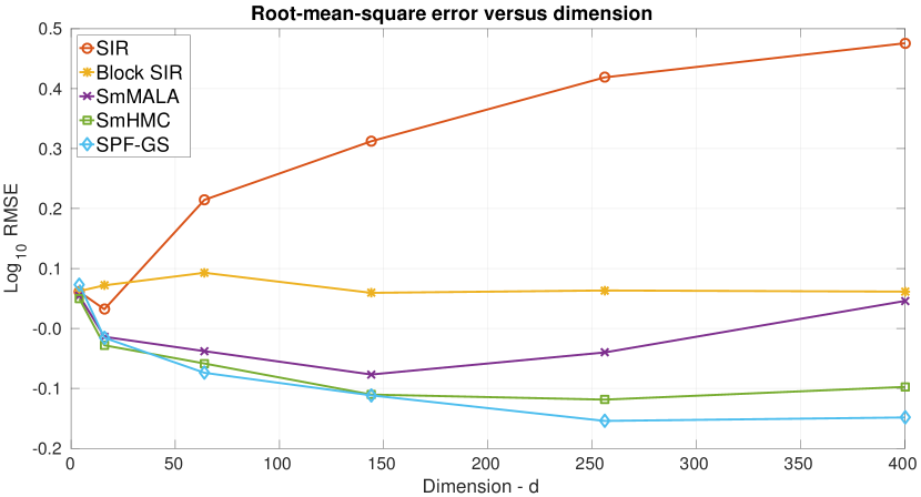
Figure 7.26: RMSE for the nonlinear, non-Gaussian sensor network example

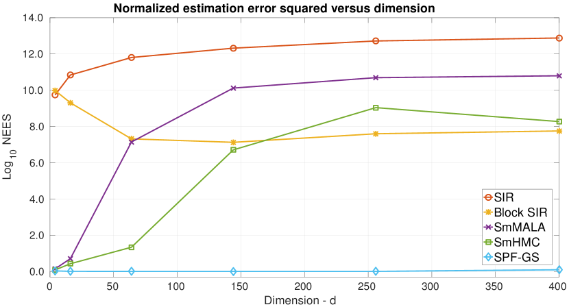
Figure 7.27: NEES for the nonlinear, non-Gaussian sensor network example

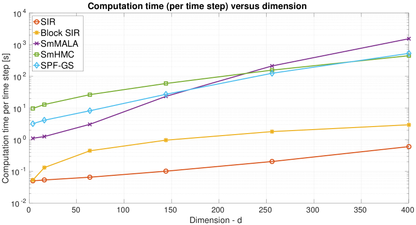
Figure 7.28: Average computation time for the nonlinear, non-Gaussian sensor network example

	Time $k=2$		Time $k=4$		Time $k=6$
	State $x(2)$	Obs. $y(2)$	State $x(4)$	Obs. $y(4)$	State $x(6)$	Obs. $y(6)$
	Post. Mean	Post. Var.	Post. Mean	Post. Var.	Post. Mean	Post. Var.
SPF-GS
SmMALA
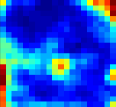
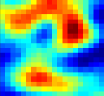
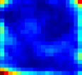
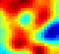
SmHMC
SIR
Block SIR

Figure 7.29: Posterior statistics for the nonlinear, non-Gaussian sensor network example ($n_{x}=400$)

8 Conclusions and Future Work

This paper builds on concepts, such as continuous-time filtering and sequential Monte Carlo methods, being intensely studied by the research community. The paper provides a description of these concepts that aims to draw out some key insights from the theoretical research into sequential Monte Carlo filtering while also responding to the significant empirical challenges encountered when applying existing and emerging tools to difficult real-world problems. More specifically, the paper is part of a growing body of research which aims to apply concepts from the sequential Monte Carlo community to problems involving high-dimensional spaces. This broader body of research and this paper in particular is motivated by the increasing demand for more statistically efficient methods to solve difficult inference problems exemplified by those involving large numbers of dimensions and relevant to a vast range of applications.

The paper capitalizes on some important findings that have been reported recently [22, 23, 56] regarding how the local properties of sequential Monte Carlo filtering measures impact algorithms’ abilities to solve high-dimensional problems. We exploit the observation made by Rebeschini & van Handel [23], that, by using the decay of correlations property, it is possible to develop particle filters based on local solutions whose approximation error becomes less sensitive to augmenting the number of state dimensions.

Within this context, we proposed a novel filter which aims to address the well-known shortcomings of sequential Monte Carlo methods when applied to nonlinear high-dimensional filtering problems. The novel method uses a Monte Carlo procedure to generate a sequence of equally-weighted samples that each guide a local solution of the Fokker-Planck equation. Using these local approximations, a mixture is produced that approximates the filtering density. The result is a statistically-sound general-purpose class of algorithms. In the context of a simple, though not trivial, high-dimensional inference problem and in comparison with state-of-the-art algorithms, the proposed approach has been shown to offer significant improvement in statistical consistency with commensurate computational expense.

In its most computationally efficient form, SPF-GS, the proposed filter has a complexity bounded by only $\mathcal{O}\left(NLn_{x}^{3}\right)$ evaluations and it has the appealing property that its operations per sample (and the associated mixture component) can be parallelized. When articulated as a marginal particle filter, SPF-MPF, the complexity is bounded by $\mathcal{O}\left(NLn_{x}^{3}+N+N^{2}\right)$ evaluations. That said, our investigations indicate that further consideration is required in order to explore fully the potential of stochastic particle flow. Future work will focus on the computational cost of the algorithms and guaranteeing certain properties of the diffusion matrix, (e.g., ensuring the matrix is positive definite and not singular). It should be possible, at least in the context of some statistical models, to reduce the computational complexity by exploiting or imposing sparsity in the diffusion matrix. Girolami & Calderhead [10] suggest that the use of guiding Hamiltonians [7] could provide a way of reducing such computational cost, but it is currently unclear how such a solution would be adopted in the context of stochastic particle flow. Another potentially promising future direction would be adopting the same approach as the well-known Broyden-Fletcher-Goldfarb-Shanno (BFGS) algorithm and thereby work around the need to explicitly evaluate the Hessian matrix at all simulation steps. We also strongly believe that it would be possible for future work to result in further improvements on the bounds used to compute the step size and number of simulation steps. Such advances will likely improve the computational efficiency of the algorithm and are the subject of ongoing development.

Appendix A Proofs

A.1 Bounds for the Time Horizon and Step Size

General Assumptions

Let $\Phi:\mathbb{R}^{n_{x}}\rightarrow\mathbb{R}$ be a measurable convex function, satisfying

$$\int_{\mathbb{R}^{n_{x}}}\exp\{-\Phi\left(\mathrm{x}\right)\} <\infty,$$ (A.1)

$$\begin{gathered}\Phi\left(\mathrm{x}\right)-\Phi\left(\bar{\mathrm{x}}\right)-\nabla_{\mathrm{x}}\Phi\left(\bar{\mathrm{x}}\right)^{T}\left(\mathrm{x}-\bar{\mathrm{x}}\right)\end{gathered} \geq\frac{1}{2}m\left\|\mathrm{x}-\bar{\mathrm{x}}\right\|_{2}^{2},$$ (A.3)

$$\left\|\nabla_{\mathrm{x}}\Phi\left(\mathrm{x}\right)-\nabla_{\mathrm{x}}\Phi\left(\bar{\mathrm{x}}\right)\right\|_{2} \leq M\left\|\mathrm{x}-\bar{\mathrm{x}}\right\|_{2},\quad\forall\mathrm{x},\bar{\mathrm{x}}\in\mathbb{R}^{n_{x}},$$ (A.4)

for two existing positive constants $m$ and $M$. Let $\bar{\mathrm{x}}\in\mathbb{R}^{n_{x}}$ be the global minimum of $\Phi\left(\mathrm{x}\right)$. We define the log-concave target density for a Langevin algorithm as $\pi(\mathrm{x})=e^{-\Phi(\mathrm{x})}\left(\int_{\mathbb{R}^{n_{x}}}e^{-\Phi(\mathrm{x})}d\mathrm{x}\right)^{-1}$.

Lemma 3.

Suppose a probability measure $\mathcal{P}_{\mathcal{L},T}$ produced by the exact integration, up to time horizon $T$, of the Langevin diffusion SDE

$$d\mathcal{L}_{\lambda}=-\frac{1}{2}D_{\lambda}\nabla\Phi(\mathcal{L}_{\lambda})d\lambda+D_{\lambda}^{1/2}dW_{\lambda},\,\lambda\geq 0,\,\mathcal{L}_{0}=0,$$ (A.5)

departing from the initial density $\nu(\mathrm{x})$ and targeting the invariant density $\pi(\mathrm{x})\propto\exp\{-\Phi(\mathrm{x})\}$ with measure $\mathcal{P}_{\pi}(d\mathrm{x})$. Process $\left\{W_{\lambda}\right\}_{\lambda\geq 0}$ is the standard Wiener process and $D_{\lambda}$ is the diffusion matrix. Under assumptions (A.1), (A.3), and (A.4),

$$\|\mathcal{P}_{\mathcal{L},T}-\mathcal{P}_{\vphantom{\mathcal{L}}\pi}\|_{\text{TV}}\leq e^{-\frac{1}{2}Tm}\mathbb{E}^{\mathcal{P}_{\pi}}\left[\nu^{2}/\pi^{2}\right]^{1/2},\,T\geq 0.$$ (A.6)

Proof.

By denoting the Markov transition kernel as $P_{t}(\mathrm{x},\cdot)$, an argument similar to that given by Dalalyan [64], invoking the Cauchy-Schwarz inequality and the spectral gap bound for the transition operator, gives

$$\|\mathcal{P}_{\mathcal{L},T}-\mathcal{P}_{\vphantom{\mathcal{L}}\pi}\|_{\text{TV}} =\sup_{\mathcal{A}\in\mathscr{B}(\mathbb{R}^{n_{x}})}\left|\int_{\mathbb{R}^{n_{x}}}P_{t}(\mathrm{x},\mathcal{A})\nu(\mathrm{x})d\mathrm{x}-\mathcal{P}_{\pi}(\mathcal{A})\right|$$

$$=\sup_{A\in\mathscr{B}(\mathbb{R}^{n_{x}})}\left|\int_{\mathbb{R}^{n_{x}}}\left(P_{t}(\mathrm{x},\mathcal{A})-\mathcal{P}_{\pi}(\mathcal{A})\right)\nu(\mathrm{x})d\mathrm{x}\right|$$

$$=\sup_{A\in\mathscr{B}(\mathbb{R}^{n_{x}})}\left|\int_{\mathbb{R}^{n_{x}}}\left(P_{t}(\mathrm{x},\mathcal{A})-\mathcal{P}_{\pi}(\mathcal{A})\right)\frac{\nu(\mathrm{x})}{\pi(\mathrm{x})}\pi(\mathrm{x})d\mathrm{x}\right|$$

$$\leq\sup_{A\in\mathscr{B}(\mathbb{R}^{n_{x}})}\int_{\mathbb{R}^{n_{x}}}\left|P_{t}(\mathrm{x},\mathcal{A})-\mathcal{P}_{\pi}(\mathcal{A})\right|\left|\frac{\nu(\mathrm{x})}{\pi(\mathrm{x})}\right|\pi(\mathrm{x})d\mathrm{x}$$

$$\leq\sup_{A\in\mathscr{B}(\mathbb{R}^{n_{x}})}\left[\int_{\mathbb{R}^{n_{x}}}\left|P_{t}(\mathrm{x},\mathcal{A})-\mathcal{P}_{\pi}(\mathcal{A})\right|^{2}\pi(\mathrm{x})d\mathrm{x}\right]^{1/2}\left(\int_{\mathbb{R}^{n_{x}}}\left|\nu(\mathrm{x})/\pi(\mathrm{x})\right|^{2}\pi(\mathrm{x})d\mathrm{x}\right)^{1/2}$$

(Dalalyan, 2014) $$\leq\frac{1}{2}e^{-\frac{1}{2}mT}\mathbb{E}^{\mathcal{P}_{\pi}}\left[\nu^{2}/\pi^{2}\right]^{1/2},$$ (A.7)

where $\mathscr{B}(\mathbb{R}^{n_{x}})$ is the $\sigma$-algebra of Borel sets of $\mathbb{R}^{n_{x}}$. ∎

Lemma 4.

Under conditions (A.1), (A.3) and (A.4), and assumptions of Lemma 3, given the initial probability density $\nu(\mathrm{x})=\mathcal{N}(\mathrm{x};\,\mu_{\nu},\sigma_{\nu}^{2}\mathbb{I}_{n_{x}})$, for $\sigma_{\nu}^{2}<2M^{-1}$, then

$$\|\mathcal{P}_{\mathcal{L},T}-\mathcal{P}_{\vphantom{\mathcal{L}}\pi}\|_{\text{TV}}\leq\frac{1}{2}\exp\left\{-\frac{1}{2}mT+\frac{n_{x}}{4}\log\left(\frac{1}{m\sigma_{\nu}^{2}(2-M\sigma_{\nu}^{2})}\right)+\frac{M}{2(2-M\sigma_{\nu}^{2})}\|\bar{\mathrm{x}}-\mu_{\nu}\|_{2}^{2}\right\}.$$ (A.8)

Proof.

According to Lemma 4 in [64], if (A.4) holds then

$$\begin{gathered}\Phi\left(\mathrm{x}\right)-\Phi\left(\bar{\mathrm{x}}\right)-\nabla_{\mathrm{x}}\Phi\left(\bar{\mathrm{x}}\right)^{T}\left(\mathrm{x}-\bar{\mathrm{x}}\right)\end{gathered}\leq\frac{M}{2}\left\|\mathrm{x}-\bar{\mathrm{x}}\right\|_{2}^{2}.$$ (A.9)

Thus,

$$\pi\left(\mathrm{x}\right) \geq e^{-\frac{M}{2}\left\|\mathrm{x}-\bar{\mathrm{x}}\right\|_{2}^{2}-\Phi\left(\bar{\mathrm{x}}\right)}\left(\int_{\mathbb{R}^{n_{x}}}e^{-\frac{m}{2}\left\|\mathrm{x}-\bar{\mathrm{x}}\right\|_{2}^{2}-\Phi\left(\bar{\mathrm{x}}\right)}d\mathrm{x}\right)^{-1}$$

$$=e^{-\frac{M}{2}\left\|\mathrm{x}-\bar{\mathrm{x}}\right\|_{2}^{2}-\Phi\left(\bar{\mathrm{x}}\right)+\Phi\left(\bar{\mathrm{x}}\right)}\left(\int_{\mathbb{R}^{n_{x}}}e^{-\frac{m}{2}\left\|\mathrm{x}-\bar{\mathrm{x}}\right\|_{2}^{2}}d\mathrm{x}\right)^{-1},$$

$$\pi\left(\mathrm{x}\right) \geq\left(2\pi m^{-1}\right)^{-n_{x}/2}e^{-\frac{M}{2}\left\|\mathrm{x}-\bar{\mathrm{x}}\right\|_{2}^{2}}.$$ (A.10)

We use (A.10), $\sigma_{\nu}^{-2}>M/2$, and define $W=2\sigma_{\nu}^{-2}$ to compute

$$\mathbb{E}^{\mathcal{P}_{\pi}}\left[\nu^{2}/\pi^{2}\right] =\int_{\mathbb{R}^{n_{x}}}\left(\frac{\nu}{\pi}\right)^{2}\pi(\mathrm{x})d\mathrm{x}=\int_{\mathbb{R}^{n_{x}}}\frac{\nu^{2}}{\pi}d\mathrm{x}$$

$$\leq\int_{\mathbb{R}^{n_{x}}}\frac{\left[\left(2\pi\sigma_{\nu}^{2}\right)^{-n_{x}/2}e^{-\frac{\sigma_{\nu}^{-2}}{2}\|\mathrm{x}-\mu_{\nu}\|_{2}^{2}}\right]^{2}}{\left(2\pi m^{-1}\right)^{-n_{x}/2}e^{-\frac{M}{2}\left\|\mathrm{x}-\bar{\mathrm{x}}\right\|_{2}^{2}}}d\mathrm{x}$$

$$=\left(2\pi\sigma_{\nu}^{2}\right)^{-n_{x}}\left(2\pi m^{-1}\right)^{n_{x}/2}\int_{\mathbb{R}^{n_{x}}}\frac{e^{-\sigma_{\nu}^{-2}\|\mathrm{x}-\mu_{\nu}\|_{2}^{2}}}{e^{-\frac{M}{2}\left\|\mathrm{x}-\bar{\mathrm{x}}\right\|_{2}^{2}}}d\mathrm{x}$$

$$=\left(2\pi\cdot 2W^{-1}\right)^{-n_{x}}\left(2\pi m^{-1}\right)^{n_{x}/2}\int_{\mathbb{R}^{n_{x}}}e^{-\frac{W}{2}\|\mathrm{x}-\mu_{\nu}\|_{2}^{2}+\frac{M}{2}\|\mathrm{x}-\bar{\mathrm{x}}\|_{2}^{2}}d\mathrm{x}$$

$$=\frac{\left(2\pi m^{-1}\right)^{n_{x}/2}}{\left(2\pi\cdot 2W^{-1}\right)^{n_{x}}}e^{\frac{1}{2}(W-M)^{-1}WM\|\bar{\mathrm{x}}-\mu_{\nu}\|_{2}^{2}}\int_{\mathbb{R}^{n_{x}}}e^{-\frac{(W-M)}{2}\|\mathrm{x}-(W-M)^{-1}(W\mu_{\nu}-M\bar{\mathrm{x}})\|_{2}^{2}}d\mathrm{x}$$

$$=\frac{\left(2\pi m^{-1}\right)^{n_{x}/2}}{\left(2\pi\cdot 2W^{-1}\right)^{n_{x}}}e^{\frac{1}{2}\left(M^{-1}-W^{-1}\right)^{-1}\|\bar{\mathrm{x}}-\mu_{\nu}\|_{2}^{2}}\left(2\pi(W-M)^{-1}\right)^{n_{x}/2}$$

$$=\left(\frac{W^{2}}{4m(W-M)}\right)^{n_{x}/2}e^{\frac{1}{2}\left(M^{-1}-W^{-1}\right)^{-1}\|\bar{\mathrm{x}}-\mu_{\nu}\|_{2}^{2}}$$

$$=\left(\frac{\sigma_{\nu}^{-4}}{m(2\sigma_{\nu}^{-2}-M)}\right)^{n_{x}/2}e^{\frac{1}{2}\left(M^{-1}-\frac{1}{2}\sigma_{\nu}^{2}\right)^{-1}\|\bar{\mathrm{x}}-\mu_{\nu}\|_{2}^{2}}$$

$$=\left(\frac{1}{m\sigma_{\nu}^{2}(2-M\sigma_{\nu}^{2})}\right)^{n_{x}/2}e^{M\left(2-M\sigma_{\nu}^{2}\right)^{-1}\|\bar{\mathrm{x}}-\mu_{\nu}\|_{2}^{2}}$$

$$\therefore\mathbb{E}^{\mathcal{P}_{\pi}}\left[\nu^{2}/\pi^{2}\right]^{1/2} \leq\exp\left\{\frac{n_{x}}{4}\log\left(\frac{1}{m\sigma_{\nu}^{2}(2-M\sigma_{\nu}^{2})}\right)+\frac{M}{2(2-M\sigma_{\nu}^{2})}\|\bar{\mathrm{x}}-\mu_{\nu}\|_{2}^{2}\right\}.$$ (A.11)

The result is complete by incorporating (A.11) into the result (A.7). ∎

Lemma 5.

For $d\nu(\mathrm{x})\sim\delta(\mathrm{x}-\mathrm{x}_{\nu})d\mathrm{x}$, the Radon-Nikodym derivative

$$\frac{d\nu}{d\mathcal{P}_{\pi}}=\frac{1}{\int_{\Omega(\mathrm{x}_{\nu})}\pi(\mathrm{x}^{\prime})d\mathrm{\mathrm{x}^{\prime}}}$$ (A.12)

is valid, where $d\mathcal{P}_{\pi}(\mathrm{x})=\pi(\mathrm{x})d\mathrm{x}$ and the integral is taken over $\Omega(\mathrm{x}_{\nu})=\left\{\mathrm{x}^{\prime}\in\mathbb{R}^{n_{x}}:\,\|\mathrm{x}^{\prime}-\bar{\mathrm{x}}\|_{2}\geq\|\mathrm{x}_{\nu}-\bar{\mathrm{x}}\|_{2}\right\}$.

Proof.

The Dirac-delta measure is singular, i.e., not absolutely continuous with respect to the Lebesgue measure, and hence its Radon-Nikodym derivative may not be formally defined in general. However, by abusing notation one can obtain a functional expression for the enunciated derivative. Observe the definition of the Radon-Nikodym derivative as

$$\frac{d\mathcal{P_{\pi}}}{d\nu}=f\implies\mathcal{P}_{\pi}(\mathcal{D})=\int_{\mathcal{D}}f\,d\nu,$$ (A.13)

for any measurable domain $\mathcal{D}\subseteq\mathbb{R}^{n_{x}}$. Given $\nu(\mathrm{x}_{\nu})=\delta(\mathrm{x}_{\nu}-\mathrm{x})\equiv\delta(\mathrm{x}-\mathrm{x}_{\nu})=\nu(\mathrm{x})$ and setting $f(\mathrm{x})\coloneqq\int_{\Omega(\mathrm{x})}\pi(\mathrm{x}^{\prime})d\mathrm{\mathrm{x}^{\prime}}$, we write

$$\mathcal{P}_{\pi}(\mathrm{x})=\int_{\mathbb{R}^{n_{x}}}f(\mathrm{x}_{\nu})\,d\nu(\mathrm{x}_{\nu})=\int_{\mathbb{R}^{n_{x}}}f(\mathrm{x}_{\nu})\,\delta(\mathrm{x}_{\nu}-\mathrm{x})d\mathrm{x}_{\nu}=f(\mathrm{x})=\int_{\Omega(\mathrm{x})}\pi(\mathrm{x}^{\prime})d\mathrm{\mathrm{x}^{\prime}},$$ (A.14)

where $\frac{d\mathcal{P}_{\pi}}{d\mathrm{x}}=\pi(\mathrm{x})$ accordingly, and $f(\mathrm{x}_{\nu})=\int_{\Omega(\mathrm{x}_{\nu})}\pi(\mathrm{x}^{\prime})d\mathrm{\mathrm{x}^{\prime}}$. Notice that $f(\mathrm{x})$ plays the role of a cumulative distribution function that is integrated over the “tail” of $\pi(\mathrm{x}^{\prime})$, in the region defined by $\Omega(\mathrm{x})$.

Thus, applying definition (A.13), we get

$$\frac{d\mathcal{P}_{\pi}}{d\nu} \coloneqq f(\mathrm{x}_{\nu})=\int_{\Omega(\mathrm{x}_{\nu})}\pi(\mathrm{x}^{\prime})d\mathrm{\mathrm{x}^{\prime}},$$

$$\therefore\frac{d\nu}{d\mathcal{P}_{\pi}} =\frac{1}{\int_{\Omega(\mathrm{x}_{\nu})}\pi(\mathrm{x}^{\prime})d\mathrm{\mathrm{x}^{\prime}}}.$$ (A.15)

∎

Remark 6.

Notice that if $\pi(\mathrm{x}^{\prime})=(2\pi P^{-1})^{-\frac{n_{x}}{2}}e^{-\frac{P}{2}\|\mathrm{x}^{\prime}-\bar{\mathrm{x}}\|_{2}^{2}}$, for some $P\in\mathbb{R}_{+}$, we can compute the resulting integral in Lemma 5 using the spherical symmetry of the Gaussian function to give

$$\int_{\Omega(\mathrm{x}_{\nu})}\pi(\mathrm{x}^{\prime})d\mathrm{\mathrm{x}^{\prime}} =(2\pi P^{-1})^{-\frac{n_{x}}{2}}\int_{\Omega(\mathrm{x}_{\nu})}e^{-\frac{P}{2}\|\mathrm{x}^{\prime}-\bar{\mathrm{x}}\|_{2}^{2}}d\mathrm{\mathrm{x}^{\prime}}$$

$$=(2\pi)^{-\frac{n_{x}}{2}}\int_{\{\|u\|_{2}\geq\sqrt{P}\|\mathrm{x}_{\nu}-\bar{\mathrm{x}}\|_{2}\}}e^{-\frac{1}{2}\|u\|_{2}^{2}}du$$

$$=(2\pi)^{-\frac{n_{x}}{2}}\int_{r_{\nu}}^{\infty}\int_{\mathcal{S}^{n_{x}-1}(r)}e^{-\frac{1}{2}r^{2}}d\mathcal{A}\,dr$$

$$=(2\pi)^{-\frac{n_{x}}{2}}\int_{r_{\nu}}^{\infty}e^{-\frac{1}{2}r^{2}}\mathcal{A}_{n_{x}-1}(r)\,dr$$

$$=(2\pi)^{-\frac{n_{x}}{2}}\mathcal{A}_{n_{x}-1}(1)\int_{r_{\nu}}^{\infty}e^{-\frac{1}{2}r^{2}}r^{n_{x}-1}\,dr$$

$$=(2\pi)^{-\frac{n_{x}}{2}}\frac{2\pi^{\frac{n_{x}}{2}}}{\Gamma\left(\frac{n_{x}}{2}\right)}\int_{r_{\nu}}^{\infty}e^{-\frac{1}{2}r^{2}}r^{n_{x}-1}\,dr$$

$$=(2\pi)^{-\frac{n_{x}}{2}}\frac{2\pi^{\frac{n_{x}}{2}}}{\Gamma\left(\frac{n_{x}}{2}\right)}2^{\frac{n_{x}}{2}-1}\int_{r_{\nu}^{2}/2}^{\infty}e^{-t}\cdot t^{\frac{n_{x}}{2}-1}\,dt$$

$$=\frac{1}{\Gamma\left(\frac{n_{x}}{2}\right)}\int_{r_{\nu}^{2}/2}^{\infty}t^{\frac{n_{x}}{2}-1}e^{-t}\,dt$$

$$=\Gamma_{u}\left(\frac{n_{x}}{2},\frac{r_{\nu}^{2}}{2}\right)=\Gamma_{u}\left(\frac{n_{x}}{2},\frac{P\|\mathrm{x}_{\nu}-\bar{\mathrm{x}}\|_{2}^{2}}{2}\right),$$

where $du=d\mathcal{A}\,dr$ for a volume element $du\in\mathbb{R}^{n_{x}}$, area element $d\mathcal{A}\in\mathbb{R}^{n_{x}-1}$ and radius element $dr\in\mathbb{R}_{+}$. In addition, $\mathcal{S}^{n_{x}-1}(r)$ denotes the $(n_{x}-1)$-sphere of radius $r$, with a total surface area of $\mathcal{A}_{n_{x}-1}(r)$, and the recursion $\mathcal{A}_{n_{x}-1}(r)=\mathcal{A}_{n_{x}-1}(1)r^{n_{x}-1}$ has been applied with $\mathcal{A}_{n_{x}-1}(1)=2\pi^{\frac{n_{x}}{2}}/\Gamma(n_{x}/2)$. The lower integration extreme is taken as $r_{\nu}\coloneqq\sqrt{P}\|\mathrm{x}_{\nu}-\bar{\mathrm{x}}\|_{2}$, and $\Gamma_{u}\left(s,x\right)=\Gamma(s)^{-1}\int_{x}^{\infty}t^{s-1}e^{-t}dt$ is the upper incomplete gamma function. Also, we recall that $\int_{\Omega(\mathrm{x}_{\nu})}\pi(\mathrm{x}^{\prime})d\mathrm{\mathrm{x}^{\prime}}=1-\int_{\mathbb{R}^{n_{x}}\setminus\Omega(\mathrm{x}_{\nu})}\pi(\mathrm{x}^{\prime})d\mathrm{\mathrm{x}^{\prime}}$.

Lemma 7.

Under conditions (A.1), (A.3) and (A.4), and assumptions of Lemma 3, given a initial probability mass located at $\mathrm{x}=\mathrm{x}_{\nu}$, i.e., $\nu(\mathrm{x})=\delta(\mathrm{x}-\mathrm{x}_{\nu})$ (Dirac delta), then

$$\|\mathcal{P}_{\mathcal{L},T}-\mathcal{P}_{\vphantom{\mathcal{L}}\pi}\|_{\text{TV}}\leq\frac{1}{2}\exp\left\{-\frac{1}{2}mT+\frac{n_{x}}{2}\log\left(\frac{M}{m}\right)-\log\left[\Gamma_{u}\left(\frac{n_{x}}{2},\frac{M\|\bar{\mathrm{x}}-\mathrm{x}_{\nu}\|_{2}^{2}}{2}\right)\right]\right\}.$$ (A.16)

Proof.

Considering $\nu(\mathrm{x})=\delta(\mathrm{x}-\mathrm{x}_{\nu})$ on the definition of total variation distance, we use Lemma 5 and Remark 6. The procedure follows as

$$\|\mathcal{P}_{\mathcal{L},T}-\mathcal{P}_{\vphantom{\mathcal{L}}\pi}\|_{\text{TV}} =\sup_{\mathcal{A}\in\mathscr{B}(\mathbb{R}^{n_{x}})}\left|\int_{\mathbb{R}^{n_{x}}}P_{t}(\mathrm{x},\mathcal{A})d\nu(\mathrm{x})-\mathcal{P}_{\pi}(\mathcal{A})\right|$$

$$=\sup_{A\in\mathscr{B}(\mathbb{R}^{n_{x}})}\left|\int_{\mathbb{R}^{n_{x}}}\left(P_{t}(\mathrm{x},\mathcal{A})-\mathcal{P}_{\pi}(\mathcal{A})\right)d\nu(\mathrm{x})\right|$$

$$=\sup_{A\in\mathscr{B}(\mathbb{R}^{n_{x}})}\left|\int_{\mathbb{R}^{n_{x}}}\left(P_{t}(\mathrm{x},\mathcal{A})-\mathcal{P}_{\pi}(\mathcal{A})\right)\frac{d\nu}{d\mathcal{P}_{\pi}}d\mathcal{P}_{\pi}(\mathrm{x})\right|$$

(Lemma 5) $$=\sup_{A\in\mathscr{B}(\mathbb{R}^{n_{x}})}\left|\int_{\mathbb{R}^{n_{x}}}\left(P_{t}(\mathrm{x},\mathcal{A})-\mathcal{P}_{\pi}(\mathcal{A})\right)\frac{1}{\int_{\Omega(\mathrm{x}_{\nu})}\pi(\mathrm{x}^{\prime})d\mathrm{\mathrm{x}^{\prime}}}d\mathcal{P}_{\pi}(\mathrm{x})\right|$$

$$\leq\frac{1}{\int_{\Omega(\mathrm{x}_{\nu})}\pi(\mathrm{x}^{\prime})d\mathrm{\mathrm{x}^{\prime}}}\cdot\sup_{A\in\mathscr{B}(\mathbb{R}^{n_{x}})}\int_{\mathbb{R}^{n_{x}}}\left|P_{t}(\mathrm{x},\mathcal{A})-\mathcal{P}_{\pi}(\mathcal{A})\right|\pi(\mathrm{x})d\mathrm{x}$$

$$\leq\frac{1}{\int_{\Omega(\mathrm{x}_{\nu})}\pi(\mathrm{x}^{\prime})d\mathrm{\mathrm{x}^{\prime}}}\cdot\sup_{A\in\mathscr{B}(\mathbb{R}^{n_{x}})}\left[\int_{\mathbb{R}^{n_{x}}}\left|P_{t}(\mathrm{x},\mathcal{A})-\mathcal{P}_{\pi}(\mathcal{A})\right|^{2}\pi(\mathrm{x})d\mathrm{x}\right]^{1/2}$$

$$\leq\frac{\left(2\pi m^{-1}\right)^{n_{x}/2}}{\int_{\Omega(\mathrm{x}_{\nu})}e^{-\frac{M}{2}\left\|\mathrm{x}^{\prime}-\bar{\mathrm{x}}\right\|_{2}^{2}}d\mathrm{x}^{\prime}}\sup_{A\in\mathscr{B}(\mathbb{R}^{n_{x}})}\left[\int_{\mathbb{R}^{n_{x}}}\left|P_{t}(\mathrm{x},\mathcal{A})-\mathcal{P}_{\pi}(\mathcal{A})\right|^{2}\pi(\mathrm{x})d\mathrm{x}\right]^{1/2}$$

$$=\frac{\left(2\pi m^{-1}\right)^{n_{x}/2}\left(2\pi M^{-1}\right)^{-n_{x}/2}}{\int_{\Omega(\mathrm{x}_{\nu})}\mathcal{N}(\mathrm{x}^{\prime};\,\bar{\mathrm{x}},M^{-1}\mathbb{I}_{n_{x}})d\mathrm{x}^{\prime}}\sup_{A\in\mathscr{B}(\mathbb{R}^{n_{x}})}\left[\int_{\mathbb{R}^{n_{x}}}\left|P_{t}(\mathrm{x},\mathcal{A})-\mathcal{P}_{\pi}(\mathcal{A})\right|^{2}\pi(\mathrm{x})d\mathrm{x}\right]^{1/2}$$

(Remark 6) $$=\frac{\left(Mm^{-1}\right)^{n_{x}/2}}{\Gamma_{u}\left(\frac{n_{x}}{2},\frac{M\|\bar{\mathrm{x}}-\mathrm{x}_{\nu}\|_{2}^{2}}{2}\right)}\sup_{A\in\mathscr{B}(\mathbb{R}^{n_{x}})}\left[\int_{\mathbb{R}^{n_{x}}}\left|P_{t}(\mathrm{x},\mathcal{A})-\mathcal{P}_{\pi}(\mathcal{A})\right|^{2}\pi(\mathrm{x})d\mathrm{x}\right]^{1/2}$$

(Dalalyan, 2014) $$\leq\left(\frac{M}{m}\right)^{n_{x}/2}\cdot\Gamma_{u}\left(\frac{n_{x}}{2},\frac{M\|\mathrm{x}_{\nu}-\bar{\mathrm{x}}\|_{2}^{2}}{2}\right)^{-1}\cdot\frac{1}{2}e^{-\frac{1}{2}mT}$$

$$=\frac{1}{2}\exp\left\{-\frac{1}{2}mT+\frac{n_{x}}{2}\log\left(\frac{M}{m}\right)-\log\left[\Gamma_{u}\left(\frac{n_{x}}{2},\frac{M\|\bar{\mathrm{x}}-\mathrm{x}_{\nu}\|_{2}^{2}}{2}\right)\right]\right\}.$$ (A.17)

∎

Lemma 8.

Suppose a probability measure $\mathcal{P}_{\tilde{\mathcal{L}}[\Delta\lambda],T}$ produced by numerical integration with step size, $\Delta\lambda$, up to time horizon $T=L\Delta\lambda$, of the Langevin diffusion SDE according to

$$d\tilde{\mathcal{L}}_{\lambda}=-\frac{1}{2}\sum_{l=0}^{L-1}D_{l\Delta\lambda}\nabla\tilde{\Phi}(\tilde{\mathcal{L}}_{l\Delta\lambda})\mathbbm{1}_{[l\Delta\lambda,(l+1)\Delta\lambda)}d\lambda+\sum_{l=0}^{L-1}D_{l\Delta\lambda}^{1/2}dW_{\lambda},\,0\leq\lambda\leq L\Delta\lambda,\,\tilde{\mathcal{L}}_{0}=\mathrm{0}.$$ (A.18)

The resulting Markov chain is assumed to depart from the initial density $\nu(\mathrm{x}_{0})=\mathcal{N}(\mathrm{x}_{0};\,\mu_{\nu},\sigma_{\nu}^{2}\mathbb{I}_{n_{x}})$ and targets the invariant density $\pi(\mathrm{x})\propto\exp\{-\Phi(\mathrm{x})\}$ with measure $\mathcal{P}_{\pi}(d\mathrm{x})$. The process $\left\{W_{\lambda}\right\}_{\lambda\geq 0}$ is the standard Wiener process and the diffusion matrix $D_{\lambda}=D(\mathrm{x}_{\lambda})$ is bounded by $K=\sup_{\mathrm{x}}\|D(\mathrm{x})\|_{2}$. Under assumptions (A.1), (A.3), and (A.4), then

$$\|\mathcal{P}_{\mathcal{L\vphantom{\tilde{\mathcal{L}}}},T}-\mathcal{P}_{\tilde{\mathcal{L}}[\Delta\lambda],T}\|_{\text{TV}}\leq\frac{1}{2}\\ -\frac{1}{2}\exp\left\{-\frac{n_{x}}{2}\frac{M^{3}K^{4}\gamma}{48(2\gamma-1)}\left(\sigma_{\nu}^{2}+\frac{1}{n_{x}}\|\mathrm{\bar{x}}-\mu_{\nu}\|_{2}^{2}+2T\right)\Delta\lambda^{2}-\frac{n_{x}M^{2}K^{3}T}{16}\Delta\lambda\right\},\,T\geq 0;$$ (A.19)

where $\mathcal{P}_{\mathcal{L},T}$ is the probability measure produced by the exact integration of the Langevin diffusion SDE.

Proof.

We take a different approach as that proposed by Dalalyan [64] for this proof. Instead of bounding the total variance distance $\|\mathcal{P}_{\mathcal{L\vphantom{\tilde{\mathcal{L}}}},T}-\mathcal{P}_{\tilde{\mathcal{L}}[\Delta\lambda],T}\|_{\text{TV}}$ by the Pinsker inequality, we treat it directly. First, identify that

$$\|\mathcal{P}_{\mathcal{L\vphantom{\tilde{\mathcal{L}}}},T}-\mathcal{P}_{\tilde{\mathcal{L}}[\Delta\lambda],T}\|_{\text{TV}} =\frac{1}{2}\int_{\mathbb{R}^{n_{x}}}\left|d\mathcal{P}_{\mathcal{L\vphantom{\tilde{\mathcal{L}}}},T}-d\mathcal{P}_{\tilde{\mathcal{L}}[\Delta\lambda],T}\right|$$

$$=\frac{1}{2}\int_{\mathbb{R}^{n_{x}}}\left|1-\frac{d\mathcal{P}_{\tilde{\mathcal{L}}[\Delta\lambda],T}}{d\mathcal{P}_{\mathcal{L},T}}\right|d\mathcal{P}_{\mathcal{L\vphantom{\tilde{\mathcal{L}}}},T}$$

$$=\frac{1}{2}\int_{\mathbb{R}^{n_{x}}}\left|1-\frac{\nu(\mathrm{x}_{0})dP_{t}^{\tilde{\mathcal{L}}}(\mathrm{x}_{0},\mathrm{x})}{\nu(\mathrm{x}_{0})dP_{t}^{\mathcal{L}}(\mathrm{x}_{0},\mathrm{x})}\right|d\mathcal{P}_{\mathcal{L},T}$$

$$=\frac{1}{2}\int_{\mathbb{R}^{n_{x}}}\left|1-\frac{dP_{t}^{\tilde{\mathcal{L}}}(\mathrm{x}_{0},\mathrm{x})}{dP_{t}^{\mathcal{L}}(\mathrm{x}_{0},\mathrm{x})}\right|d\mathcal{P}_{\mathcal{L},T}(\mathrm{x})$$

$$=\frac{1}{2}\int_{\mathbb{R}^{n_{x}}}\mathbb{E}^{P_{t}^{\mathcal{L}}}\left[\left|1-\frac{dP_{t}^{\tilde{\mathcal{L}}}(\mathrm{x}_{0},\mathrm{x})}{dP_{t}^{\mathcal{L}}(\mathrm{x}_{0},\mathrm{x})}\right||\mathrm{x}_{0}\right]d\nu(\mathrm{x}_{0}),$$ (A.20)

where $\mathcal{P}_{\mathcal{L},T}(d\mathrm{x})=\int_{\mathbb{R}^{n_{x}}}P_{t}^{\mathcal{L}}(\mathrm{x}_{0},d\mathrm{x})\nu(\mathrm{x}_{0})d\mathrm{x}_{0}$, and $P_{t}^{\tilde{\mathcal{L}}}(\mathrm{x}_{0},\cdot)$ and $P_{t}^{\mathcal{L}}(\mathrm{x}_{0},\cdot)$ are the Markov transition kernels for the discrete-time and continuous-time Langevin dynamics respectively. By applying Girsanov’s theorem to change the measure from $\mathcal{P}_{\mathcal{L\vphantom{\tilde{\mathcal{L}}}},T}$ to $\mathcal{P}_{\tilde{\mathcal{L}}[\Delta\lambda],T}$, one obtains (see step 3 of the proof of Proposition 2 in [91])

$$\frac{dP_{t}^{\tilde{\mathcal{L}}}}{dP_{t}^{\mathcal{L}}}(\mathrm{x})\\ =\exp\left\{\int_{0}^{T}\frac{1}{2}\left(-\sum_{l=0}^{L-1}D_{l\Delta\lambda}\nabla\tilde{\Phi}(\mathrm{x}_{l\Delta\lambda})\mathbbm{1}_{[l\Delta\lambda,(l+1)\Delta\lambda)}+D_{\lambda}\nabla\Phi(\mathrm{x}_{\lambda})\right)^{T}D_{\lambda}^{-1}\left(d\mathcal{L}_{\lambda}+\frac{1}{2}D_{\lambda}\nabla\Phi(\mathcal{L}_{\lambda})d\lambda\right)\right\}\\ \times\exp\left\{-\frac{1}{2}\int_{0}^{T}\left\|-\frac{1}{2}\sum_{l=0}^{L-1}D_{l\Delta\lambda}\nabla\tilde{\Phi}(\mathrm{x}_{l\Delta\lambda})\mathbbm{1}_{[l\Delta\lambda,(l+1)\Delta\lambda)}+\frac{1}{2}D_{\lambda}\nabla\Phi(\mathrm{x}_{\lambda})\right\|_{2}^{2}d\lambda\right\}.$$ (A.21)

Thus, since $\mathbb{E}\left[e^{z}\right]\geq e^{\mathbb{E}\left[z\right]}$ by Jensen’s inequality, $D_{\lambda}=D(\mathrm{x}_{\lambda})\leq K$, and $\nabla\Phi(\mathrm{x})$ is Lipschitz-continuous with constant $M$ (A.4), we obtain

$$\mathbb{E}^{P_{t}^{\mathcal{L}}}\left[\frac{dP_{t}^{\tilde{\mathcal{L}}}}{dP_{t}^{\mathcal{L}}}(\mathrm{x})|\mathrm{x}_{0}\right] \geq\exp\left\{-\mathbb{E}^{P_{t}^{\mathcal{L}}}\left[\frac{1}{2}\sum_{l=0}^{L-1}\int_{l\Delta\lambda}^{(l+1)\Delta\lambda}\left\|\frac{1}{2}D_{\lambda}\nabla\Phi(\mathrm{x}_{\lambda})-\frac{1}{2}D_{l\Delta\lambda}\nabla\tilde{\Phi}(\mathrm{x}_{l\Delta\lambda})\right\|_{2}^{2}d\lambda|\mathrm{x}_{0}\right]\right\}$$

$$=\exp\left\{-\frac{1}{2}\sum_{l=0}^{L-1}\int_{l\Delta\lambda}^{(l+1)\Delta\lambda}\mathbb{E}^{P_{t}^{\mathcal{L}}}\left[\left\|\frac{1}{2}D_{\lambda}\nabla\Phi(\mathrm{x}_{\lambda})-\frac{1}{2}D_{l\Delta\lambda}\nabla\tilde{\Phi}(\mathrm{x}_{l\Delta\lambda})\right\|_{2}^{2}|\mathrm{x}_{0}\right]d\lambda\right\}$$

$$\geq\exp\left\{-\frac{K^{2}}{8}\sum_{l=0}^{L-1}\int_{l\Delta\lambda}^{(l+1)\Delta\lambda}\mathbb{E}^{P_{t}^{\mathcal{L}}}\left[\left\|\nabla\Phi(\mathrm{x}_{\lambda})-\nabla\tilde{\Phi}(\mathrm{x}_{l\Delta\lambda})\right\|_{2}^{2}|\mathrm{x}_{0}\right]d\lambda\right\}$$

$$\geq\exp\left\{-\frac{K^{2}M^{2}}{8}\sum_{l=0}^{L-1}\int_{l\Delta\lambda}^{(l+1)\Delta\lambda}\mathbb{E}^{P_{t}^{\mathcal{L}}}\left[\left\|\mathrm{x}_{\lambda}-\mathrm{x}_{l\Delta\lambda}\right\|_{2}^{2}|\mathrm{x}_{0}\right]d\lambda\right\}.$$ (A.22)

For each step $\mathrm{x}_{\lambda}-\mathrm{x}_{l\Delta\lambda}=-\frac{1}{2}D_{l\Delta\lambda}\nabla\Phi(\mathrm{x}_{l\Delta\lambda})(\lambda-l\Delta\lambda)+D_{l\Delta\lambda}^{1/2}(W_{\lambda}-W_{l\Delta\lambda})$, hence

$$\mathbb{E}^{P_{t}^{\mathcal{L}}}\left[\frac{dP_{t}^{\tilde{\mathcal{L}}}}{dP_{t}^{\mathcal{L}}}(\mathrm{x})|\mathrm{x}_{0}\right] \geq\exp\left\{-\frac{K^{2}M^{2}}{8}\sum_{l=0}^{L-1}\int_{l\Delta\lambda}^{(l+1)\Delta\lambda}\mathbb{E}^{P_{t}^{\mathcal{L}}}\left[\left\|\frac{1}{2}D(\mathrm{x}_{l\Delta\lambda})\nabla\Phi(\mathrm{x}_{l\Delta\lambda})\right\|_{2}^{2}(\lambda-l\Delta\lambda)^{2}|\mathrm{x}_{0}\right]d\lambda\right\}$$

$$\times\exp\left\{-\frac{K^{2}M^{2}}{8}\sum_{l=0}^{L-1}\int_{l\Delta\lambda}^{(l+1)\Delta\lambda}\mathbb{E}^{P_{t}^{\mathcal{L}}}\left[\left\|D(\mathrm{x}_{l\Delta\lambda})^{1/2}(W_{\lambda}-W_{l\Delta\lambda})\right\|_{2}^{2}|\mathrm{x}_{0}\right]d\lambda\right\}$$

$$\geq\exp\left\{-\frac{K^{2}M^{2}}{8}\sum_{l=0}^{L-1}\int_{l\Delta\lambda}^{(l+1)\Delta\lambda}\frac{K^{2}}{4}\mathbb{E}^{P_{t}^{\mathcal{L}}}\left[\|\nabla\Phi(\mathrm{x}_{l\Delta\lambda})\|_{2}^{2}|\mathrm{x}_{0}\right](\lambda-l\Delta\lambda)^{2}d\lambda\right\}$$

$$\times\exp\left\{-\frac{K^{2}M^{2}}{8}\sum_{l=0}^{L-1}\int_{l\Delta\lambda}^{(l+1)\Delta\lambda}K(\lambda-l\Delta\lambda)n_{x}d\lambda\right\}$$

$$=\exp\left\{-\frac{M^{2}K^{4}\Delta\lambda^{3}}{96}\sum_{l=0}^{L-1}\mathbb{E}^{P_{t}^{\mathcal{L}}}\left[\|\nabla\Phi(\mathrm{x}_{l\Delta\lambda})\|_{2}^{2}|\mathrm{x}_{0}\right]-\frac{n_{x}M^{2}K^{3}L\Delta\lambda^{2}}{16}\right\}.$$ (A.23)

Now we invoke a result from Corollary 4 in [64], that gives

$$\Delta\lambda\sum_{l=0}^{L-1}\mathbb{E}\left[\|\nabla\Phi(\mathrm{x}_{l\Delta\lambda})\|_{2}^{2}\right]\leq\frac{M\gamma}{2\gamma-1}\mathbb{E}\left[\|\mathrm{x}_{0}-\bar{\mathrm{x}}\|_{2}^{2}\right]+\frac{2\gamma MTn_{x}}{2\gamma-1},$$ (A.24)

for some $\gamma>1$, $\Delta\lambda\leq(\gamma M)^{-1}$ and $L>1$. Substituting $L\Delta\lambda=T$ and incorporating (A.24):

$$\mathbb{E}^{P_{t}^{\mathcal{L}}}\left[\frac{dP_{t}^{\tilde{\mathcal{L}}}}{dP_{t}^{\mathcal{L}}}(\mathrm{x})|\mathrm{x}_{0}\right] \geq\exp\left\{-\frac{M^{2}K^{4}\Delta\lambda^{2}}{48}\frac{\gamma}{2\gamma-1}\left(\frac{M}{2}\mathbb{E}^{P_{t}^{\mathcal{L}}}\left[\|\mathrm{x}_{0}-\bar{\mathrm{x}}\|_{2}^{2}|\mathrm{x}_{0}\right]+n_{x}MT\right)-\frac{n_{x}M^{2}K^{3}T\Delta\lambda}{16}\right\}$$

$$=\exp\left\{-\frac{M^{2}K^{4}\Delta\lambda^{2}}{48}\frac{\gamma}{2\gamma-1}\left(\frac{M}{2}\|\mathrm{x}_{0}-\bar{\mathrm{x}}\|_{2}^{2}+n_{x}MT\right)-\frac{n_{x}M^{2}K^{3}T\Delta\lambda}{16}\right\}.$$ (A.25)

Since

$$0\leq\mathbb{E}^{P_{t}^{\mathcal{L}}}\left[\frac{dP_{t}^{\tilde{\mathcal{L}}}}{dP_{t}^{\mathcal{L}}}(\mathrm{x})|\mathrm{x}_{0}\right]\leq 1,$$

and applying expression (A.25) in (A.20), we have

$$\|\mathcal{P}_{\mathcal{L\vphantom{\tilde{\mathcal{L}}}},T}-\mathcal{P}_{\tilde{\mathcal{L}}[\Delta\lambda],T}\|_{\text{TV}} =\frac{1}{2}\int_{\mathbb{R}^{n_{x}}}\left|1-\frac{dP_{t}^{\tilde{\mathcal{L}}}(\mathrm{x}_{0},\mathrm{x})}{dP_{t}^{\mathcal{L}}(\mathrm{x}_{0},\mathrm{x})}\right|d\mathcal{P}_{\mathcal{L},T}(\mathrm{x})$$

$$=\frac{1}{2}\int_{\mathbb{R}^{n_{x}}}d\mathcal{P}_{\mathcal{L},T}(\mathrm{x})-\frac{1}{2}\int_{\mathbb{R}^{n_{x}}}\mathbb{E}^{P_{t}^{\mathcal{L}}}\left[\frac{dP_{t}^{\tilde{\mathcal{L}}}(\mathrm{x}_{0},\mathrm{x})}{dP_{t}^{\mathcal{L}}(\mathrm{x}_{0},\mathrm{x})}|\mathrm{x}_{0}\right]d\nu(\mathrm{x}_{0})$$

$$\leq\frac{1}{2}-\frac{1}{2}\int_{\mathbb{R}^{n_{x}}}e^{-\frac{M^{2}K^{4}\Delta\lambda^{2}}{48}\frac{\gamma}{2\gamma-1}\left(\frac{M}{2}\|\mathrm{x}_{0}-\bar{\mathrm{x}}\|_{2}^{2}+n_{x}MT\right)-\frac{n_{x}M^{2}K^{3}T\Delta\lambda}{16}}\nu(\mathrm{x}_{0})d\mathrm{x}_{0}.$$ (A.26)

Finally, using the substitutions $A_{1}=\frac{M^{3}K^{4}}{96}\frac{\gamma}{2\gamma-1}$, $A_{2}=\frac{n_{x}M^{3}TK^{4}}{48}\frac{\gamma}{2\gamma-1}$, $B=\frac{n_{x}M^{2}K^{3}T}{16}$, $\mathbb{E}\left[e^{-z}\right]\geq e^{-\mathbb{E}\left[z\right]}$ by Jensen’s inequality, and $\nu(\mathrm{x}_{0})=\mathcal{N}(\mathrm{x}_{0};\,\mu_{\nu},\sigma_{\nu}^{2}\mathbb{I}_{n_{x}})$, we get

$$\|\mathcal{P}_{\mathcal{L\vphantom{\tilde{\mathcal{L}}}},T}-\mathcal{P}_{\tilde{\mathcal{L}}[\Delta\lambda],T}\|_{\text{TV}} \leq\frac{1}{2}-\frac{1}{2}e^{-A_{2}\Delta\lambda^{2}-B\Delta\lambda}\int_{\mathbb{R}^{n_{x}}}e^{-A_{1}\Delta\lambda^{2}\|\mathrm{x}_{0}-\bar{\mathrm{x}}\|_{2}^{2}}\nu(\mathrm{x}_{0})d\mathrm{x}_{0}$$

$$\leq\frac{1}{2}-\frac{1}{2}e^{-A_{2}\Delta\lambda^{2}-B\Delta\lambda}e^{-A_{1}\Delta\lambda^{2}\int_{\mathbb{R}^{n_{x}}}\|\mathrm{x}_{0}-\bar{\mathrm{x}}\|_{2}^{2}\nu(\mathrm{x}_{0})d\mathrm{x}_{0}}$$

$$=\frac{1}{2}-\frac{1}{2}e^{-A_{2}\Delta\lambda^{2}-B\Delta\lambda-A_{1}\Delta\lambda^{2}\left(n_{x}\sigma_{\nu}^{2}+\|\mathrm{\bar{x}}-\mu_{\nu}\|_{2}^{2}\right)}$$

$$=\frac{1}{2}-\frac{1}{2}e^{-\left(A_{1}\left(n_{x}\sigma_{\nu}^{2}+\|\mathrm{\bar{x}}-\mu_{\nu}\|_{2}^{2}\right)+A_{2}\right)\Delta\lambda^{2}-B\Delta\lambda}$$

$$=\frac{1}{2}-\frac{1}{2}e^{-\frac{n_{x}}{2}\frac{M^{3}K^{4}\gamma}{48(2\gamma-1)}\left(\sigma_{\nu}^{2}+\frac{1}{n_{x}}\|\mathrm{\bar{x}}-\mu_{\nu}\|_{2}^{2}+2T\right)\Delta\lambda^{2}-\frac{n_{x}M^{2}K^{3}T}{16}\Delta\lambda}.$$ (A.27)

∎

Lemma 9.

Under the same assumptions as of Lemma 8, except for a initial density $\nu(\mathrm{x}_{0})=\delta(\mathrm{x}_{0}-\mathrm{x}_{\nu})$ (Dirac delta), i.e., a probability mass initially located at $\mathrm{x}_{0}=\mathrm{x}_{\nu}$, then

$$\|\mathcal{P}_{\mathcal{L\vphantom{\tilde{\mathcal{L}}}},T}-\mathcal{P}_{\tilde{\mathcal{L}}[\Delta\lambda],T}\|_{\text{TV}}\leq\frac{1}{2}\\ -\frac{1}{2}\exp\left\{-\frac{n_{x}}{2}\frac{M^{3}K^{4}\gamma}{48(2\gamma-1)}\left(\frac{1}{n_{x}}\|\mathrm{\bar{x}}-\mathrm{x}_{\nu}\|_{2}^{2}+2T\right)\Delta\lambda^{2}-\frac{n_{x}M^{2}K^{3}T}{16}\Delta\lambda\right\},\,T\geq 0;$$ (A.28)

Proof.

The proof follows straightforwardly by substituting $\nu(\mathrm{x}_{0})=\delta(\mathrm{x}_{0}-\mathrm{x}_{\nu})$ into (A.26). ∎

Theorem 10.

Let a convex function $\Phi$ satisfy the general assumptions (A.1), (A.3) and (A.4). Suppose a discrete-time Langevin Monte Carlo algorithm integrates (4.15), targeting the invariant density $\pi(\mathrm{x})\propto\exp\{-\Phi(\mathrm{x})\}$ with measure $\mathcal{P}_{\pi}(d\mathrm{x})$. In addition, assume that for some $\gamma\geq 1$ we have $\Delta\lambda\leq\left(\gamma M\right)^{-1}$, and $K=\sup_{\mathrm{x}}\|D(\mathrm{x})\|_{2}$ where $D_{\lambda}=D(\mathrm{x}_{\lambda})$ is the diffusion matrix. Then, for a time horizon, $T$, and step size, $\Delta\lambda$, the total-variation distance between the target measure $\mathcal{P}_{\pi}$ and the approximated measure $\mathcal{P}_{\mathcal{\tilde{\mathcal{L}}}(\Delta\lambda),T}$ furnished by a discrete-time Langevin Monte Carlo algorithm with initial density $\nu\left(\mathrm{x}\right)=\mathcal{N}(\mathrm{x};\mu_{\nu},\sigma_{\nu}^{2}\mathbb{I}_{n_{x}})$, for $\sigma_{\nu}^{2}<2M^{-1}$, satisfies

$$\|\mathcal{P}_{\mathcal{\tilde{\mathcal{L}}}[\Delta\lambda],T}-\mathcal{P}_{\vphantom{\tilde{\mathcal{L}}}\pi}\|_{\text{TV}}\leq\frac{1}{2}\exp\left\{-\frac{1}{2}mT+\frac{n_{x}}{4}\log\left(\frac{1}{m\sigma_{\nu}^{2}(2-M\sigma_{\nu}^{2})}\right)+\frac{M}{2(2-M\sigma_{\nu}^{2})}\|\bar{\mathrm{x}}-\mu_{\nu}\|_{2}^{2}\right\}\\ +\frac{1}{2}-\frac{1}{2}\exp\left\{-\frac{n_{x}}{2}\frac{M^{3}K^{4}\gamma}{48(2\gamma-1)}\left(\sigma_{\nu}^{2}+\frac{1}{n_{x}}\|\mathrm{\bar{x}}-\mu_{\nu}\|_{2}^{2}+2T\right)\Delta\lambda^{2}-\frac{n_{x}M^{2}K^{3}T}{16}\Delta\lambda\right\}.$$ (A.29)

Proof.

The proof follows from the triangle inequality

$$\|\mathcal{P}_{\tilde{\mathcal{L}}[\Delta\lambda],T}-\mathcal{P}_{\vphantom{\tilde{\mathcal{L}}}\pi}\|_{\text{TV}}\leq\|\mathcal{P}_{\mathcal{L\vphantom{\tilde{\mathcal{L}}}},T}-\mathcal{P}_{\vphantom{\tilde{\mathcal{L}}}\pi}\|_{\text{TV}}+\|\mathcal{P}_{\mathcal{L\vphantom{\tilde{\mathcal{L}}}},T}-\mathcal{P}_{\tilde{\mathcal{L}}[\Delta\lambda],T}\|_{\text{TV}},$$ (A.30)

on which we subsitute the results of Lemmas 4 and 8 to give the final result (A.29). ∎

Corollary 11.

Let $n_{x}\geq 2$, $\Phi$ satisfy (A.1), (A.3) and (A.4), and $\varepsilon\in(0,\nicefrac{{1}}{{2}})$ be a desired precision level. Let the time horizon, $T$, and the step size, $\Delta\lambda$, be defined by

$$T \geq\frac{2\log\left(1/\varepsilon\right)+\frac{n_{x}}{2}\log\left(\frac{1}{m\sigma_{\nu}^{2}(2-M\sigma_{\nu}^{2})}\right)+\frac{M}{(2-M\sigma_{\nu}^{2})}\|\bar{\mathrm{x}}-\mu_{\nu}\|_{2}^{2}}{m},$$ (A.31)

$$\Delta\lambda \leq\frac{-\frac{T}{16}+\sqrt{\left(\frac{T}{16}\right)^{2}+\frac{\gamma}{48(2\gamma-1)}\left(\sigma_{\nu}^{2}+\frac{1}{n_{x}}\|\mathrm{\bar{x}}-\mu_{\nu}\|_{2}^{2}+2T\right)M^{-1}K^{-2}\left[\frac{2}{n_{x}}\log\left(\frac{1}{1-\varepsilon}\right)\right]}}{\frac{\gamma}{48(2\gamma-1)}\left(\sigma_{\nu}^{2}+\frac{1}{n_{x}}\|\mathrm{\bar{x}}-\mu_{\nu}\|_{2}^{2}+2T\right)MK},$$ (A.32)

where $\gamma\geq 1$. Then the resulting probability distribution of a Langevin Monte Carlo algorithm that integrates (4.15) after $L=\left\lceil T/\Delta\lambda\right\rceil$ steps, satisfies $\|\mathcal{P}_{\mathcal{\tilde{\mathcal{L}}}[\Delta\lambda],T}-\mathcal{P}_{\vphantom{\tilde{\mathcal{L}}}\pi}\|_{\text{TV}}\leq\varepsilon$.

Proof.

Bound each term on the right-hand side of (A.30) by half of the required precision $\varepsilon$, i.e.,

$$\|\mathcal{P}_{\mathcal{L\vphantom{\tilde{\mathcal{L}}}},T}-\mathcal{P}_{\vphantom{\tilde{\mathcal{L}}}\pi}\|_{\text{TV}}\leq\varepsilon/2,\,\|\mathcal{P}_{\mathcal{L\vphantom{\tilde{\mathcal{L}}}},T}-\mathcal{P}_{\tilde{\mathcal{L}}[\Delta\lambda],T}\|_{\text{TV}}\leq\varepsilon/2.$$

For the first term:

$$\frac{1}{2}\exp\left\{-\frac{1}{2}mT+\frac{n_{x}}{4}\log\left(\frac{1}{m\sigma_{\nu}^{2}(2-M\sigma_{\nu}^{2})}\right)+\frac{M}{2(2-M\sigma_{\nu}^{2})}\|\bar{\mathrm{x}}-\mu_{\nu}\|_{2}^{2}\right\}\leq\frac{\varepsilon}{2},\\ -\frac{1}{2}mT+\frac{n_{x}}{4}\log\left(\frac{1}{m\sigma_{\nu}^{2}(2-M\sigma_{\nu}^{2})}\right)+\frac{M}{2(2-M\sigma_{\nu}^{2})}\|\bar{\mathrm{x}}-\mu_{\nu}\|_{2}^{2}\leq\log\varepsilon,\\ \frac{1}{2}mT\geq-\log\varepsilon+\frac{n_{x}}{4}\log\left(\frac{1}{m\sigma_{\nu}^{2}(2-M\sigma_{\nu}^{2})}\right)+\frac{M}{2(2-M\sigma_{\nu}^{2})}\|\bar{\mathrm{x}}-\mu_{\nu}\|_{2}^{2},\\ T\geq\frac{2\log\left(1/\varepsilon\right)+\frac{n_{x}}{2}\log\left(\frac{1}{m\sigma_{\nu}^{2}(2-M\sigma_{\nu}^{2})}\right)+\frac{M}{(2-M\sigma_{\nu}^{2})}\|\bar{\mathrm{x}}-\mu_{\nu}\|_{2}^{2}}{m}.$$ (A.33)

And for the second term:

$$\frac{1}{2}-\frac{1}{2}\exp\left\{\vphantom{\frac{n_{x}}{2}\frac{M^{3}K^{4}\gamma}{48(2\gamma-1)}\left(\sigma_{\nu}^{2}+\frac{1}{n_{x}}\|\mathrm{\bar{x}}-\mu_{\nu}\|_{2}^{2}+2T\right)}\smash{-\overbrace{\frac{n_{x}}{2}\frac{M^{3}K^{4}\gamma}{48(2\gamma-1)}\left(\sigma_{\nu}^{2}+\frac{1}{n_{x}}\|\mathrm{\bar{x}}-\mu_{\nu}\|_{2}^{2}+2T\right)}^{a\,(>0)}\Delta\lambda^{2}-\overbrace{\frac{n_{x}M^{2}K^{3}T}{16}}^{b\,(>0)}\Delta\lambda}\right\}\leq\frac{\varepsilon}{2},\\ \exp\left\{-a\Delta\lambda^{2}-b\Delta\lambda\right\}\geq 1-\varepsilon,\\ -a\Delta\lambda^{2}-b\Delta\lambda\geq\log\left(1-\varepsilon\right),\\ a\Delta\lambda^{2}+b\Delta\lambda\leq-\log\left(1-\varepsilon\right),\\ a\Delta\lambda^{2}+b\Delta\lambda+c\leq 0,\,c=\log\left(1-\varepsilon\right)=-\log\left(\frac{1}{1-\varepsilon}\right),\\ 0<\Delta\lambda\leq\frac{-b+\sqrt{b^{2}-4ac}}{2a},\\ \Delta\lambda\leq\frac{-\frac{n_{x}M^{2}K^{3}T}{16}+\sqrt{\left(\frac{n_{x}M^{2}K^{3}T}{16}\right)^{2}+4\frac{n_{x}}{2}\frac{M^{3}K^{4}\gamma}{48(2\gamma-1)}\left(\sigma_{\nu}^{2}+\frac{1}{n_{x}}\|\mathrm{\bar{x}}-\mu_{\nu}\|_{2}^{2}+2T\right)\log\left(\frac{1}{1-\varepsilon}\right)}}{2\frac{n_{x}}{2}\frac{M^{3}K^{4}\gamma}{48(2\gamma-1)}\left(\sigma_{\nu}^{2}+\frac{1}{n_{x}}\|\mathrm{\bar{x}}-\mu_{\nu}\|_{2}^{2}+2T\right)},\\ \Delta\lambda\leq\frac{-\frac{T}{16}+\sqrt{\left(\frac{T}{16}\right)^{2}+\frac{\gamma}{48(2\gamma-1)}\left(\sigma_{\nu}^{2}+\frac{1}{n_{x}}\|\mathrm{\bar{x}}-\mu_{\nu}\|_{2}^{2}+2T\right)M^{-1}K^{-2}\left[\frac{2}{n_{x}}\log\left(\frac{1}{1-\varepsilon}\right)\right]}}{\frac{\gamma}{48(2\gamma-1)}\left(\sigma_{\nu}^{2}+\frac{1}{n_{x}}\|\mathrm{\bar{x}}-\mu_{\nu}\|_{2}^{2}+2T\right)MK}.$$ (A.34)

∎

Proof of Theorem 1

Proof.

We follow the same procedure established for proving Theorem 10, subsituting the results of Lemmas 7 and 9 into (A.30) to give

$$\|\mathcal{P}_{\tilde{\mathcal{L}}[\Delta\lambda],T}-\mathcal{P}_{\pi}\|_{\text{TV}}\leq\frac{1}{2}\exp\left\{-\frac{1}{2}mT+\frac{n_{x}}{2}\log\left(\frac{M}{m}\right)-\log\left[\Gamma_{u}\left(\frac{n_{x}}{2},\frac{M\|\bar{\mathrm{x}}-\mathrm{x}_{\nu}\|_{2}^{2}}{2}\right)\right]\right\}\\ +\frac{1}{2}-\frac{1}{2}\exp\left\{-\frac{n_{x}}{2}\frac{M^{3}K^{4}\gamma}{48(2\gamma-1)}\left(\frac{1}{n_{x}}\|\mathrm{\bar{x}}-\mathrm{x}_{\nu}\|_{2}^{2}+2T\right)\Delta\lambda^{2}-\frac{n_{x}M^{2}K^{3}T}{16}\Delta\lambda\right\}.$$ (A.35)

∎

Proof of Corollary 2

Proof.

We follow the same procedure established for proving Corollary 11, bounding each term on the right-hand side of (A.30) in view of (A.35) to obtain

$$T \geq\frac{2\log\left(1/\varepsilon\right)+n_{x}\log\left(\frac{M}{m}\right)-2\log\left[\Gamma_{u}\left(\frac{n_{x}}{2},\frac{M\|\bar{\mathrm{x}}-\mathrm{x}_{\nu}\|_{2}^{2}}{2}\right)\right]}{m},$$ (A.36)

$$\Delta\lambda \leq\frac{-\frac{T}{16}+\sqrt{\left(\frac{T}{16}\right)^{2}+\frac{\gamma}{48(2\gamma-1)}\left(\frac{1}{n_{x}}\|\mathrm{\bar{x}}-\mathrm{x}_{\nu}\|_{2}^{2}+2T\right)M^{-1}K^{-2}\left[\frac{2}{n_{x}}\log\left(\frac{1}{1-\varepsilon}\right)\right]}}{\frac{\gamma}{48(2\gamma-1)}\left(\frac{1}{n_{x}}\|\mathrm{\bar{x}}-\mathrm{x}_{\nu}\|_{2}^{2}+2T\right)MK}.$$ (A.37)

∎

A.2 On the Filtering Properties of the Stochastic Particle Flow

Theorem 12.

Define $\mathrm{x}\in\mathbb{R}^{n_{x}}$ to describe an $n_{x}$-dimensional vector state. Let the vector field $\mu:\mathbb{R}^{n_{x}}\rightarrow\mathbb{R}^{n_{x}}$, $\mu\left(\mathrm{x}\right)\in\mathcal{C}^{1}(\mathbb{R}^{n_{x}})$, be a conservative field, i.e., there exists a scalar potential function $\psi:\mathbb{R}^{n_{x}}\rightarrow\mathbb{R}$, $\psi\left(\mathrm{x}\right)\in\mathcal{C}^{2}(\mathbb{R}^{n_{x}}),$ such that

$$\mu\left(\mathrm{x}\right)=-\nabla_{\mathrm{x}}\psi\left(\mathrm{x}\right).$$ (A.38)

Let $p\left(\mathrm{x},\lambda\right)$ be the density of an ensemble of particles and, without loss of generality, can be assumed to be a continuous probability density function on $\mathbb{R}^{n_{x}}$ that depends on the pseudo-time variable $\lambda\in\mathbb{R}$, $\lambda\geq 0$. Set $\pi\left(\mathrm{x}\right)\propto e^{-\psi\left(\mathrm{x}\right)}$ to be an invariant, locally log-concave probability density to which the density $p\left(\mathrm{x},\lambda\right)$ is expected to converge weakly at a stationary state in a finite time horizon $\lambda\geq T$, $T\in\mathbb{R}_{+}$, i.e.,

$$\mathbb{E}_{p}\left[\varphi\left(\mathrm{x}\right)\right]\rightarrow\mathbb{E}_{\pi}\left[\varphi\left(\mathrm{x}\right)\right],\quad\lambda\rightarrow T;$$ (A.39)

for all bounded, continuous functions $\varphi$, and where $\mathbb{E}_{p}\left[.\right]$ is the expectation with respect to the probability density $p\left(\mathrm{x},\lambda\right)$. If the probability density $p\left(\mathrm{x},\lambda\right)$ satisfies the continuity equation (Liouville’s equation)

$$\frac{\partial p}{\partial\lambda}=-\nabla_{\mathrm{x}}\cdot\left(p\,\mu\right),\quad\lambda\geq 0;$$ (A.40)

with the initial condition

$$p\left(\mathrm{x},\lambda\right)=p_{0}\left(\mathrm{x}\right),\quad\lambda=0;$$ (A.41)

then any probability mass (particle) $\mathrm{x}_{m}\left(0\right)\sim p_{0}\left(\mathrm{x}\right)$, when evolved according to the associated state equation

$$d\mathrm{x}_{m}(\lambda)=\mu\left(\mathrm{x}_{m}(\lambda)\right)d\lambda,\quad\lambda\geq 0;$$ (A.42)

converges to

$$\mathrm{x}_{m}\left(T\right)=\text{argmax}\left[\pi\left(\mathrm{x}\right)\right],\quad\lambda\geq T,$$ (A.43)

at a stable equilibrium.

Proof.

The general solution of the continuity equation without sources (A.40) assumes the form (see for example [92])

$$p\left(\mathrm{x},\lambda\right) =p_{0}\left(\mathrm{x}_{m}(\mathrm{x},\lambda)\right)\left|\frac{\partial\mathrm{x}_{m}}{\partial\mathrm{x}}\right|$$

$$=p_{0}\left(\mathrm{x}_{m}(\mathrm{x},\lambda)\right)\left|\mathcal{J}_{\mathrm{x}}\left[\mathrm{x}_{m}(\mathrm{x},\lambda)\right]\right|,$$ (A.44)

where $\mathrm{x}_{m}(\mathrm{x},\lambda)$ is an arbitrary element of mass that is regarded as a function of the pseudo-time $\lambda$ and of the state $\mathrm{x}$ that it can possibly reach. The matrix $\mathcal{J}_{\mathrm{x}}\left[\mathrm{x}_{m}(\mathrm{x},\lambda)\right]$ is the Jacobian matrix of $\mathrm{x}_{m}(\mathrm{x},\lambda)$ with respect to $\mathrm{x}$. Conceptually, at the stationary state $\mathrm{x}_{m}\left(\mathrm{x}_{T},T\right)=\mathrm{x}_{T}$ the continuity equation (A.40) reads

$$\frac{\partial p}{\partial\lambda}=0,\quad\lambda\geq T.$$ (A.45)

Using the general solution (A.44) to verify the stationary condition (A.45), we conclude that

$$p_{0}\left(\mathrm{x}_{m}(\mathrm{x}_{T},T)\right)\left|\mathcal{J}_{\mathrm{x}}\left[\mathrm{x}_{m}(\mathrm{x}_{T},T)\right]\right|$$

must be constant with respect to the pseudo-time, thus

$$\frac{d\mathrm{x}_{m}(\lambda)}{d\lambda}=\mu\left(\mathrm{x}_{m}(\lambda)\right)=0,\quad\lambda\geq T.$$ (A.46)

Following the assumption of conservative field, $\mu\left(\mathrm{x}_{T}\right)=-\nabla_{\mathrm{x}}\psi\left(\mathrm{x}_{T}\right)=0$ implies that the stationary state $\mathrm{x}_{T}$ is an equilibrium point, i.e., an extreme of the potential function $\psi$. In addition, since the potential function is assumed to be related to the stationary distribution as ${\psi\left(\mathrm{x}\right)\propto-\log\pi\left(\mathrm{x}\right)}$, the stationary state $\mathrm{x}_{T}$ is an extreme of the stationary density.

A valid Lyapunov function of the flow is $V\left(\mathrm{x}\right)=\psi\left(\mathrm{x}\right)$, which is positive semi-definite ($\psi\left(\mathrm{x}\right)\geq 0$) in the neighbourhood of the equilibrium point due to the local log-concavity of the invariant density $\pi\left(\mathrm{x}\right)$. Analysing the (Lie) time derivative of the Lyapunov function in the neighbourhood of the equilibrium point, $\left\|\mathrm{x}-\mathrm{x}_{T}\right\|<\varepsilon$ for a sufficiently small $\varepsilon\in\mathbb{R}_{+}$, we have

$$\frac{dV\left(\mathrm{x}\right)}{d\lambda} =\nabla_{\mathrm{x}}V\left(\mathrm{x}\right)^{T}\cdot\frac{d\mathrm{x}}{d\lambda}=\nabla_{\mathrm{x}}V\left(\mathrm{x}\right)^{T}\cdot\mu\left(\mathrm{x}\right),$$

$$\dot{V}\left(\mathrm{x}\right) =\nabla_{\mathrm{x}}\psi\left(\mathrm{x}\right)^{T}\cdot\left(-\nabla_{\mathrm{x}}\psi\left(\mathrm{x}\right)\right),$$

$$\dot{V}\left(\mathrm{x}\right) =-\left\|\nabla_{\mathrm{x}}\psi\left(\mathrm{x}\right)\right\|^{2}\leq 0,\,\left\|\mathrm{x}-\mathrm{x}_{T}\right\|<\varepsilon;$$ (A.47)

from which we conclude that $\mathrm{x}_{T}$ is a point of (uniformily) stable equilibrium. Therefore, under the established hypotheses, any arbitrary probability mass $\mathrm{x}_{m}\left(\lambda\right)$ evolved according to (A.42) converges to

$$\mathrm{x}_{m}\left(T\right) =\text{argmin}\left[\psi\left(\mathrm{x}\right)\right]=\text{argmin}\left[-\log\pi\left(\mathrm{x}\right)\right],$$

$$\mathrm{x}_{m}\left(T\right) =\text{argmax}\left[\pi\left(\mathrm{x}\right)\right],\quad\lambda\geq T;$$

at a stable equilibrium. ∎

Lemma 13.

Let $\left\{\mathrm{X}_{\lambda}:t\leq\lambda\leq T\right\}$ be a diffusion process in $\mathbb{R}^{n_{x}}$ (hence a Markov process), solution of

$$d\mathrm{X}_{\lambda} =\mu_{f}\left(\mathrm{X}_{\lambda},\lambda\right)d\lambda+D_{f}\left(\lambda\right)^{\nicefrac{{1}}{{2}}}dW_{\lambda},$$ (A.48)

$$\hphantom{=\ }\mathrm{X}_{\lambda}\left(t\right)=\mathrm{x}_{t},t\leq\lambda\leq T;$$

where $\left\{W_{\lambda}:t\leq\lambda\leq T\right\}$ is a standard Wiener process in $\mathbb{R}^{n_{x}}$ under the probability measure $\mathcal{P}$, $\mu_{f}:\mathbb{R}^{n_{x}}\times[t,T]\rightarrow\mathbb{R}^{n_{x}}$ is the drift and $D_{f}:[t,T]\rightarrow\mathbb{R}^{n_{x}\times n_{x}}$ is a diffusion coefficient invariant over the space at any time instant. There exists an equivalent process $\left\{\bar{\mathrm{X}}_{\tau},\mathcal{V}_{\tau}:t\leq\tau\leq T\right\}$, which is probabilistically the same as the original process, called reverse process on the interval $[t,T]$ (see [93]), that provides the solution of the stochastic system

$$d\bar{\mathrm{X}}_{\tau} =\mu_{r}\left(\bar{\mathrm{X}}_{\tau},\tau\right)d\tau+D_{r}\left(\tau\right)^{\nicefrac{{1}}{{2}}}d\bar{W}_{\tau},\>\bar{\mathrm{X}}_{\tau}\left(t\right)=\bar{x}_{t};$$ (A.49)

$$d\mathcal{V}_{\tau} =v_{r}\left(\bar{\mathrm{X}}_{\tau},\tau\right)\mathcal{V}_{\tau}d\tau,\hphantom{D_{r}\left(\tau\right)^{\nicefrac{{1}}{{2}}}d\bar{W}_{\tau}^{P}\,\,\,\,}\mathcal{V}_{\tau}\left(t\right)=1;$$ (A.50)

for a standard Wiener process $\left\{\bar{W}_{\tau}:t\leq\tau\leq T\right\}$ in $\mathbb{R}^{n_{x}}$ under the measure $\mathcal{P}$, with the reverse drift and diffusion coefficients given, respectively, by

$$\mu_{r}\left(\bar{\mathrm{X}}_{\tau},\tau\right) =-\mu_{f}\left(\bar{\mathrm{X}}_{\tau},T+t-\lambda\right),$$ (A.51)

$$D_{r}\left(\tau\right) =\hphantom{-}D_{f}\left(T+t-\lambda\right).$$ (A.52)

Proof.

The Markov process $\left\{\mathrm{X}_{\lambda}\right\}$, as an existing solution to the SDE (A.48), has an associated probability density $p\left(\mathrm{x}_{\lambda},\lambda\right)$ that must satisfy the Kolmogorov forward equation (Fokker-Planck equation):

$$\frac{\partial}{\partial\lambda}p =-\nabla_{\mathrm{x}}\cdot\left(\mu_{f}p\right)+\frac{1}{2}\nabla_{\mathrm{x}}\cdot\left(D_{f}\nabla_{\mathrm{x}}p\right),\,\lambda\geq t,$$

$$\hphantom{=-\ }p\left(\mathrm{x}_{\lambda},t\right)=p_{t}\left(\mathrm{x}_{t}\right),\mathrm{x}_{\lambda}\in\mathbb{R}^{n_{x}}.$$

The Fokker-Planck equation can be written in the non-divergence form as

$$\frac{\partial}{\partial\lambda}p=\hat{\mu}^{T}\nabla_{\mathrm{x}}p+\frac{1}{2}\nabla_{\mathrm{x}}\cdot\left(D_{f}\nabla_{\mathrm{x}}p\right)+\hat{v}\cdot p,$$ (A.53)

where

$$\hat{\mu}\left(\mathrm{x}_{\lambda}\right) =-\mu_{f}\left(\mathrm{x}_{\lambda}\right),$$

$$\hat{v}\left(\mathrm{x}_{\lambda}\right) =-\nabla_{\mathrm{x}}\cdot\mu_{f}\left(\mathrm{x}_{\lambda}\right).$$

We introduce the reverse time variable $\tau=T+t-\lambda$, so that

$$p\left(\mathrm{x}_{\lambda}(T+t-\lambda),T+t-\lambda\right)\equiv\hat{p}\left(\bar{\mathrm{x}}_{\tau},\tau\right),$$

and hence $-\partial_{\lambda}p=\partial_{\tau}\hat{p}$. Thus, rewritting (A.53) with respect to $\hat{p}\left(\bar{\mathrm{x}}_{\tau},\tau\right)$ for $\tau\leq T$, $\bar{\mathrm{x}}_{\tau}\in\mathbb{R}^{n_{x}}$, and performing the substitutions

$$\mu_{r}\left(\bar{\mathrm{x}}_{\tau},\tau\right) =-\mu_{f}\left(\mathrm{x}_{\lambda}(T+t-\lambda),T+t-\lambda\right),$$

$$D_{r}\left(\tau\right) =\hphantom{-}D_{f}\left(T+t-\lambda\right),$$

we obtain

$$\frac{\partial}{\partial\lambda}p =-\mu_{f}^{T}\nabla_{\mathrm{x}}p+\frac{1}{2}\nabla_{\mathrm{x}}\cdot\left(D_{f}\nabla_{\mathrm{x}}p\right)+\left(-\nabla_{\mathrm{x}}\cdot\mu_{f}\right)\cdot p,$$

$$-\frac{\partial}{\partial\tau}\hat{p} =\hphantom{-}\mu_{r}^{T}\nabla_{\bar{\mathrm{x}}}\hat{p}+\frac{1}{2}\nabla_{\bar{\mathrm{x}}}\cdot\left(D_{r}\nabla_{\bar{\mathrm{x}}}\hat{p}\right)-\left(-\nabla_{\bar{\mathrm{x}}}\cdot\mu_{r}\right)\cdot\hat{p},$$

$$-\frac{\partial}{\partial\tau}\hat{p} =\hphantom{-}\mu_{r}^{T}\nabla_{\bar{\mathrm{x}}}\hat{p}+\frac{1}{2}\nabla_{\bar{\mathrm{x}}}\cdot\left(D_{r}\nabla_{\bar{\mathrm{x}}}\hat{p}\right)-v_{r}\cdot\hat{p},\,\tau\leq T,$$ (A.54)

$$\hphantom{=-\ }\hat{p}\left(\bar{\mathrm{x}}_{\tau},T\right)=\hat{p}_{T}\left(\bar{\mathrm{x}}_{T}\right)=p_{t}\left(\mathrm{x}_{t}\right),\bar{\mathrm{x}}_{\tau}\in\mathbb{R}^{n_{x}};$$

where

$$v_{r}\left(\bar{\mathrm{x}}_{\tau},\tau\right)=-\nabla_{\bar{\mathrm{x}}}\mu_{r}\left(\bar{\mathrm{x}}_{\tau},\tau\right).$$ (A.55)

Solving (A.54) corresponds to the Cauchy problem in reverse time $\tau\leq T$, which is equivalent to solve the stochastic system stated by (A.49) and (A.50). Therefore, because the solution to the SDE (A.48) is assumed to exist and corresponds to the solution of (A.54) for $\tau\leq T$, then there exists the equivalent reverse process $\left\{\bar{\mathrm{X}}_{\tau},\mathcal{V}_{\tau}\right\}_{\tau\in[t,T]}$ that solves the stochastic system (A.49) and (A.50). ∎

Remark 14.

Despite its name, inherited from [93], it is worth stressing that $\left\{\bar{\mathrm{X}}_{\tau},\mathcal{V}_{\tau}\right\}$ is the solution of a stochastic system forward in time on the interval $[t,T]$, which may be properly understood as a smoothing process.

Remark 15.

It is clear that the solution of (A.50) at $\tau=T$ is

$$\mathcal{V}_{T}\equiv\mathcal{V}_{\tau}\left(T\right)=e^{-\int_{t}^{T}v_{r}\left(\bar{\mathrm{x}}_{\tau},\tau\right)d\tau},$$

which evokes the solution of (A.54) by the Feynman-Kac formula

$$\hat{p}\left(\mathrm{x},\tau\right)=\mathbb{E}^{\mathcal{P}}\left[e^{-\int_{\tau}^{T}v_{r}\left(\bar{\mathrm{x}}_{\tau^{\prime}},\tau^{\prime}\right)d\tau^{\prime}}\hat{p}_{T}\left(\bar{\mathrm{x}}_{T}\right)|\bar{\mathrm{x}}_{\tau}=\mathrm{x}\right].$$ (A.56)

A more general form of the Lemma 13 can be found in [93].

Lemma 16.

The reverse process $\left\{\bar{\mathrm{X}}_{\tau},\mathcal{V}_{\tau}:t\leq\tau\leq T\right\}$ described by (A.49) and (A.50), has an associated smooth probability density $\hat{p}\left(\bar{\mathrm{x}}_{\tau},\tau\right)$ that satisfies, for the initial value problem, the Kolmogorov forward equation

$$\frac{\partial}{\partial\tau}\hat{p} =-\nabla_{\bar{\mathrm{x}}}\cdot\left(\mu_{r}\hat{p}\right)+\frac{1}{2}\nabla_{\bar{\mathrm{x}}}\cdot\left(D_{r}\nabla_{\bar{\mathrm{x}}}\hat{p}\right)-v_{r}\cdot\hat{p},\,t\leq\tau\leq T,$$ (A.57)

$$\hphantom{=-\ }\hat{p}\left(\bar{\mathrm{x}}_{\tau}(t),\tau=t\right)=\hat{p}_{t}\left(\bar{\mathrm{x}}_{t}\right),\bar{\mathrm{x}}_{\tau}\in\mathbb{R}^{n_{x}}.$$

Proof.

We consider a continuous function of the process $\left\{\bar{\mathrm{X}}_{\tau},\mathcal{V}_{\tau}\right\}_{\tau\in[t,T]}$, declared as $\varphi:\mathbb{R}^{n_{x}}\times\mathbb{R}\rightarrow\mathbb{R}$, which is assumed to be $\varphi(\bar{\mathrm{X}}_{\tau},\mathcal{V}_{\tau})\in\mathcal{C}^{2}(\mathbb{R}^{n_{x}},\mathbb{R})$, bounded and integrable on the product space $\mathbb{R}^{n_{x}}\times\mathbb{R}$. Applying Îto’s lemma to $\varphi$ and substituting (A.49) and (A.50) one obtains

$$d\varphi =(\nabla_{\bar{\mathrm{X}}_{\tau}}\varphi)^{T}d\bar{\mathrm{X}}_{\tau}+\frac{1}{2}d\bar{\mathrm{X}}_{\tau}^{T}\mathcal{H}_{\bar{\mathrm{X}}_{\tau}}\left[\varphi\right]d\bar{\mathrm{X}}_{\tau}+\partial_{\mathcal{V}_{\tau}}\varphi\,d\mathcal{V}_{\tau}$$

$$=(\nabla_{\bar{\mathrm{X}}_{\tau}}\varphi)^{T}\cdot\left(\mu_{r}d\tau+D_{r}{}^{\nicefrac{{1}}{{2}}}d\bar{W}_{\tau}\right)+\frac{1}{2}\text{tr}\left\{D_{r}\mathcal{H}_{\bar{\mathrm{X}}_{\tau}}\left[\varphi\right]\right\}d\tau+\partial_{\mathcal{V}_{\tau}}\varphi\cdot\left(v_{r}\mathcal{V}_{\tau}d\tau\right),$$

$$=\left[(\nabla_{\bar{\mathrm{X}}_{\tau}}\varphi)^{T}\mu_{r}+\frac{1}{2}\text{tr}\left\{D_{r}\mathcal{H}_{\bar{\mathrm{X}}_{\tau}}\left[\varphi\right]\right\}+\partial_{\mathcal{V}_{\tau}}\varphi\cdot v_{r}\mathcal{V}_{\tau}\right]d\tau+(\nabla_{\bar{\mathrm{X}}_{\tau}}\varphi)^{T}D_{r}{}^{\nicefrac{{1}}{{2}}}d\bar{W}_{\tau}.$$ (A.58)

Consider the expected (average) rate of change of the projections of $\varphi$ defined by:

$$\left\langle\dot{\varphi}_{\mathcal{V}}\right\rangle\left(\tau\right) \triangleq\left\langle\frac{d}{d\tau}\int_{1}^{\mathcal{V}_{T}}\varphi(\bar{\mathrm{X}}_{\tau},\mathcal{V}_{\tau})d\mathcal{V}_{\tau}\right\rangle$$

$$=\left\langle\int_{1}^{\mathcal{V}_{T}}\partial_{\tau}\varphi(\bar{\mathrm{X}}_{\tau},\mathcal{V}_{\tau})d\mathcal{V}_{\tau}\right\rangle$$

$$\equiv\int_{\mathbb{R}^{n_{x}}}\int_{1}^{\upsilon_{T}}\varphi\left(\bar{\mathrm{x}}_{\tau},\upsilon_{\tau}\right)\cdot\partial_{\tau}\hat{p}\,d\upsilon_{\tau}d\bar{\mathrm{x}}_{\tau}.$$ (A.59)

Substituting (A.58) into (A.59), we have

$$\left\langle\dot{\varphi}_{\mathcal{V}}\right\rangle\left(\tau\right) =\left\langle\int_{1}^{\mathcal{V}_{T}}\partial_{\tau}\varphi(\bar{\mathrm{X}}_{\tau},\mathcal{V}_{\tau})d\mathcal{V}_{\tau}\right\rangle$$

$$=\left\langle\int_{1}^{\mathcal{V}_{T}}\left[(\nabla_{\bar{\mathrm{X}}_{\tau}}\varphi)^{T}\mu_{r}+\frac{1}{2}\text{tr}\left\{D_{r}\mathcal{H}_{\bar{\mathrm{X}}_{\tau}}\left[\varphi\right]\right\}+\partial_{\mathcal{V}_{\tau}}\varphi\cdot v_{r}\mathcal{V}_{\tau}\right]d\mathcal{V}_{\tau}\right\rangle$$

$$=\int_{1}^{\upsilon_{T}}\int_{\mathbb{R}^{n_{x}}}\left[(\nabla_{\bar{\mathrm{x}}_{\tau}}\varphi)^{T}\mu_{r}+\frac{1}{2}\text{tr}\left\{D_{r}\mathcal{H}_{\bar{\mathrm{x}}_{\tau}}\left[\varphi\right]\right\}\right]\hat{p}\,d\bar{\mathrm{x}}_{\tau}d\upsilon_{\tau}$$

$$+\int_{\mathbb{R}^{n_{x}}}\int_{1}^{\upsilon_{T}}\left[\partial_{\mathcal{\upsilon}_{\tau}}\varphi\,\cdot v_{r}\,\upsilon_{\tau}\right]\hat{p}\,d\upsilon_{\tau}d\bar{\mathrm{x}}_{\tau}.$$ (A.60)

Integrating (A.60) by parts and offsetting the integration constant to cancel out the surface terms, we have

$$\left\langle\dot{\varphi}_{\mathcal{V}}\right\rangle\left(\tau\right) =\int_{1}^{\upsilon_{T}}\int_{\mathbb{R}^{n_{x}}}\varphi\cdot\left[-\nabla_{\bar{\mathrm{x}}_{\tau}}\cdot(\mu_{r}\hat{p})+\frac{1}{2}\nabla_{\bar{\mathrm{x}}_{\tau}}\cdot\left(D_{r}\nabla_{\bar{\mathrm{x}}_{\tau}}\hat{p}\right)\right]\,d\bar{\mathrm{x}}_{\tau}d\upsilon_{\tau}$$

$$+\int_{\mathbb{R}^{n_{x}}}\int_{1}^{\upsilon_{T}}\varphi\cdot\left[-v_{r}\partial_{\upsilon_{\tau}}(\upsilon_{\tau}\hat{p})\right]\,d\upsilon_{\tau}d\bar{\mathrm{x}}_{\tau}$$

$$=\int_{\mathbb{R}^{n_{x}}}\int_{1}^{\upsilon_{T}}\varphi\cdot\left[-\nabla_{\bar{\mathrm{x}}_{\tau}}\cdot(\mu_{r}\hat{p})+\frac{1}{2}\nabla_{\bar{\mathrm{x}}_{\tau}}\cdot\left(D_{r}\nabla_{\bar{\mathrm{x}}_{\tau}}\hat{p}\right)\right]\,d\upsilon_{\tau}d\bar{\mathrm{x}}_{\tau}$$

$$+\int_{\mathbb{R}^{n_{x}}}\int_{1}^{\upsilon_{T}}\varphi\cdot\left[-v_{r}\hat{p}\right]\,d\upsilon_{\tau}d\bar{\mathrm{x}}_{\tau}$$

$$=\int_{\mathbb{R}^{n_{x}}}\int_{1}^{\upsilon_{T}}\varphi\cdot\left[-\nabla_{\bar{\mathrm{x}}_{\tau}}\cdot(\mu_{r}\hat{p})+\frac{1}{2}\nabla_{\bar{\mathrm{x}}_{\tau}}\cdot\left(D_{r}\nabla_{\bar{\mathrm{x}}_{\tau}}\hat{p}\right)-v_{r}\hat{p}\right]\,d\upsilon_{\tau}d\bar{\mathrm{x}}_{\tau}.$$ (A.61)

The proof of the lemma is complete by comparing (A.61) to the definition (A.59) and noting that their integrands must be equal. ∎

Theorem 17.

Let $\left(\Omega,\mathcal{F},\mathcal{P}\right)$ to be a complete probability space and let $\left\{\mathcal{F}_{\lambda}\right\}_{\lambda\geq 0}$, $\lambda\in[0,T]$, be an increasing family of sub $\sigma$-fields of $\mathcal{F}$. Let $\left\{\mathrm{X}_{\lambda}:0<\lambda\leq T\right\}$ be an $\mathcal{F}_{\lambda}$-adapted process, considered to be the signal process with state equation

$$d\mathrm{X}_{\lambda} =\mu_{f}\left(\mathrm{X}_{\lambda}\right)d\lambda+D_{f}\left(\lambda\right)^{\nicefrac{{1}}{{2}}}dW_{\lambda},$$ (A.62)

$$\hphantom{=\ }\mathrm{X}_{\lambda}\left(0\right)=\mathrm{x}_{0},\,0\leq\lambda\leq T;$$

for a Wiener process $\left\{W_{\lambda}\right\}_{\lambda\in[0,T]}$ under the probability measure $\mathcal{P}$. Assume $p(\mathrm{x}_{\lambda},\lambda)$ defined on $\left(\Omega,\mathcal{F}\right)$ to be the probability density of the measure $\mathcal{P}$, which

(a) is the probabilistic representation of the process $\left\{\mathrm{X}_{\lambda}\right\}_{\lambda\in[0,T]}$,

(b) is absolutely continuous with respect to the Lesbesque measure,

(c) approaches a stationary measure as ${p(\mathrm{x}_{\lambda})\stackrel{{\scriptstyle\lambda\rightarrow T}}{{\longrightarrow}}\pi\left(\mathrm{x}_{\lambda}\right)\propto e^{-\Phi\left(\mathrm{x}_{\lambda}\right)}}$, for a sufficiently long horizon $T$.

Let $\left\{\bar{X}_{\tau},\mathcal{V}_{\tau}:\lambda<\tau\leq T\right\}$ be the reverse process of $\left\{\mathrm{X}_{\lambda}\right\}_{\lambda\in[0,T]}$, as established in Lemma 13 by the stochastic system (A.49) and (A.50), so that the reverse drift and diffusion coefficients are, respectively,

$$\mu_{r}\left(\bar{\mathrm{x}}_{\tau}\right) =-\frac{1}{2}D_{r}\left(\lambda\right)\nabla_{\bar{\mathrm{x}}}\log\pi\left(\bar{\mathrm{x}}_{\tau}\right),$$

$$D_{r}\left(\tau\right) =\left[-\mathcal{H}_{\bar{\mathrm{x}}}\left[\log\pi\left(\bar{\mathrm{x}}_{\tau}\right)\right]\right]^{-1}.$$

Assume $\hat{p}(\bar{\mathrm{x}}_{\tau},\tau)$ to be the probability density on $\left(\Omega,\mathcal{F}\right)$ describing the reverse process $\left\{\bar{X}_{\tau},\mathcal{V}_{\tau}\right\}_{\tau\in[\lambda,T]}$, under the same measure $\mathcal{P}$, which must satisfy the Kolmogorov forward equation (provided a known initial condition) according to Lemma 16:

$$\frac{\partial}{\partial\tau}\hat{p} =-\nabla_{\bar{\mathrm{x}}}\cdot\left(\mu_{r}\hat{p}\right)+\frac{1}{2}\nabla_{\bar{\mathrm{x}}}\cdot\left(D_{r}\nabla_{\bar{\mathrm{x}}}\hat{p}\right)-v_{r}\cdot\hat{p},\,\lambda\leq\tau\leq T,$$ (A.63)

$$\hphantom{=-\ }\hat{p}\left(\bar{\mathrm{x}}_{\tau}\left(\lambda\right),\tau=\lambda\right)=\hat{p}_{\lambda}\left(\bar{\mathrm{x}}_{\tau}\left(\lambda\right)\right)=\pi\left(\mathrm{x}_{T}\right),\bar{\mathrm{x}}_{\tau}\in\Omega;$$

If the stationary density is set to be

$$\pi\left(\mathrm{x}\right)\coloneqq\frac{p\left(\mathrm{y}_{k}|\mathrm{x}\right)p\left(\mathrm{x}|\mathrm{y}_{1:k-1}\right)}{Z_{1}}=\frac{p\left(\mathrm{y}_{k}|\mathrm{x}\right)p_{x}\left(\mathrm{x}\right)}{Z_{1}},$$ (A.64)

where the prior density $p_{x}\left(\mathrm{x}\right)$ and the likelihood $p\left(\mathrm{y}_{k}|\mathrm{x}\right)$ are integrable functions with respect to $\mathrm{x}$, $Z_{1}=p\left(\mathrm{y}_{k}|\mathrm{y}_{1:k-1}\right)$ is a normalization constant, and the discrete-time observation process $\left\{\mathrm{y}_{k}\in\mathbb{R}^{n_{y}}:k\in\mathbb{N}\right\}$ is described as

$$\mathrm{y}_{k}=h\left(\mathrm{x}_{k}\right)+R^{\nicefrac{{1}}{{2}}}\xi_{k},\quad\xi_{k}\sim\mathcal{N}(\xi_{k};0_{n_{y}},\mathrm{I}_{n_{y}});$$ (A.65)

then the probability density corresponding to the signal process (A.62) is equivalent to the following filtering entity

$$p(\mathrm{x},\lambda|\mathcal{F}_{\lambda})=\frac{\mathbb{E}^{P}\left[e^{h\left(\mathrm{x}_{T}\right)^{T}R^{-1}\mathrm{y}_{k}-\frac{1}{2}h\left(\mathrm{x}_{T}\right)^{T}R^{-1}h\left(\mathrm{x}_{T}\right)}|\mathrm{x}\right]p\left(\mathrm{x}|\mathrm{y}_{1:k-1}\right)}{Z}.$$ (A.66)

In addition, the expression (A.66) can be interpreted as the analogous to the well known result (see [94])

$$p(\mathrm{x},\lambda|\mathcal{F}_{\lambda})=\frac{\mathbb{E}^{P}\left[e^{\int_{0}^{T}h_{T}\left(\mathrm{x}_{\lambda}\right)^{T}R_{T}^{-1}d\mathrm{y_{\lambda}}-\frac{1}{2}\int_{0}^{T}h_{T}\left(\mathrm{x}_{\lambda}\right)^{T}R_{T}^{-1}h_{T}\left(\mathrm{x}_{\lambda}\right)d\lambda}|\mathrm{x}\right]}{Z}p\left(\mathrm{x}|\mathrm{y}_{1:k-1}\right),$$ (A.67)

for a discrete-time observation process whose analog continuous-time (interpolated) version has the observation function $h_{T}\left(.\right)$ and covariance matrix $R_{T}$.

Proof.

By definition of the stochastic system described by (A.49) and (A.50), and Lemma 16, the reverse process $\left\{\bar{X}_{\tau},\mathcal{V}_{\tau}\right\}$ is known to satisfy the Kolmogorov forward equation (A.63) in reverse time $\lambda\leq\tau\leq T$, for which the stationary density $\pi$ is an initial condition (initial value problem). Using the reverse time variable $\tau=T-\lambda$, so that $p\left(\mathrm{x}_{\lambda},\lambda\right)\equiv\hat{p}\left(\bar{\mathrm{x}}_{\tau}(T-\tau),T-\tau\right)$ and ${\partial_{\lambda}p=-\partial_{\tau}\hat{p}}$, and applying the relations (A.51), (A.52) and (A.55) from Lemma 13, we rewrite the equation (A.63) for $0\leq\lambda\leq T$ as

$$\frac{\partial}{\partial\tau}\hat{p} =-\nabla_{\bar{\mathrm{x}}}\cdot\left(\mu_{r}\hat{p}\right)+\frac{1}{2}\nabla_{\bar{\mathrm{x}}}\cdot\left(D_{r}\nabla_{\bar{\mathrm{x}}}\hat{p}\right)-v_{r}\cdot\hat{p},\,\lambda\leq\tau\leq T,$$

$$\frac{\partial}{\partial\tau}\hat{p} =-\left(\nabla_{\bar{\mathrm{x}}}\cdot\mu_{r}\right)\hat{p}-\mu_{r}^{T}\nabla_{\bar{\mathrm{x}}}\hat{p}+\frac{1}{2}\nabla_{\bar{\mathrm{x}}}\cdot\left(D_{r}\nabla_{\bar{\mathrm{x}}}\hat{p}\right)+\left(\nabla_{\bar{\mathrm{x}}}\cdot\mu_{r}\right)\hat{p},$$

$$\frac{\partial}{\partial\tau}\hat{p} =-\mu_{r}^{T}\nabla_{\bar{\mathrm{x}}}\hat{p}+\frac{1}{2}\nabla_{\bar{\mathrm{x}}}\cdot\left(D_{r}\nabla_{\bar{\mathrm{x}}}\hat{p}\right),$$

$$-\frac{\partial}{\partial\lambda}p =+\mu_{f}^{T}\nabla_{\mathrm{x}}p+\frac{1}{2}\nabla_{\mathrm{x}}\cdot\left(D_{f}\nabla_{\mathrm{x}}p\right),\,0\leq\lambda\leq T,$$ (A.68)

$$\hphantom{=+\ }p\left(\mathrm{x}_{\lambda},T\right)=\pi\left(\mathrm{x}_{T}\right),\mathrm{x}_{\lambda}\in\Omega.$$

Now we have a Kolmogorov backward equation in $p\left(\mathrm{x}_{\lambda},\lambda\right)$ with a terminal value problem for the forward process $\left\{\mathrm{X}_{\lambda}\right\}$. Hence, we can apply the Feynman-Kac formula for the terminal condition $p(\mathrm{x},T)=\pi\left(\mathrm{x}\right)$, with $\mathrm{x}_{T}=\mathrm{x}_{\lambda}(T)$, to give

$$p(\mathrm{x},\lambda) \triangleq\mathbb{E}^{\mathcal{P}}\left[\pi\left(\mathrm{x}_{T}\right)|\mathrm{x}_{\lambda}=\mathrm{x}\right]$$

$$=\frac{\mathbb{E}^{\mathcal{P}}\left[p\left(\mathrm{y}_{k}|\mathrm{x}_{T}\right)p\left(\mathrm{x}_{T}|\mathrm{y}_{1:k-1}\right)|\mathrm{x}_{\lambda}=\mathrm{x}\right]}{Z_{1}}$$

$$=\frac{\mathbb{E}^{\mathcal{P}}\left[e^{-\frac{1}{2}\left(\mathrm{y}_{k}-h\left(\mathrm{x}_{T}\right)\right)^{T}R^{-1}\left(\mathrm{y}_{k}-h\left(\mathrm{x}_{T}\right)\right)}p_{x}\left(\mathrm{x}_{T}\right)|\mathrm{x}\right]}{Z_{1}\left(2\pi R\right)^{\nicefrac{{n_{y}}}{{2}}}}$$

$$=\frac{\mathbb{E}^{\mathcal{P}}\left[e^{h\left(\mathrm{x}_{T}\right)^{T}R^{-1}\mathrm{y}_{k}-\frac{1}{2}h\left(\mathrm{x}_{T}\right)^{T}R^{-1}h\left(\mathrm{x}_{T}\right)}p_{x}\left(\mathrm{x}_{T}\right)|\mathrm{x}\right]}{Z_{1}\left(2\pi R\right)^{\nicefrac{{n_{y}}}{{2}}}e^{+\frac{1}{2}\mathrm{y}_{k}^{T}R^{-1}\mathrm{y}_{k}^{\vphantom{T}}}}$$

$$=\frac{\mathbb{E}^{\mathcal{P}}\left[e^{h\left(\mathrm{x}_{T}\right)^{T}R^{-1}\mathrm{y}_{k}-\frac{1}{2}h\left(\mathrm{x}_{T}\right)^{T}R^{-1}h\left(\mathrm{x}_{T}\right)}p_{x}\left(\mathrm{x}_{T}\right)|\mathcal{F}_{\lambda},\mathrm{x}\right]}{Z}.$$ (A.69)

Let us reinterpret the discrete-time observation process as a continuous-time process for which we only obtain a realization at $\lambda=T$, by linearly interpolating it along the interval $0<\lambda\leq T$ to write

$$d\mathrm{y_{\lambda}} = \frac{1}{T}h\left(\mathrm{x}_{\lambda}\right)d\lambda+\left(\frac{R}{T}\right)^{\nicefrac{{1}}{{2}}}\xi_{k}d\lambda^{\nicefrac{{1}}{{2}}},$$

$$d\mathrm{y_{\lambda}^{\mathcal{Q}}} = h_{T}\left(\mathrm{x}_{\lambda}\right)d\lambda+R_{T}^{\nicefrac{{1}}{{2}}}d\bar{\xi}_{\lambda}^{\mathcal{P}},\quad 0<\lambda\leq T.$$ (A.70)

where $\left\{\bar{\xi}_{\lambda}\right\}$ is an interpolated Wiener process, under the probability measure $\mathcal{P}$, that produces the observation noise $\int_{0}^{T}R_{T}^{\nicefrac{{1}}{{2}}}d\bar{\xi}_{\lambda}\equiv R^{\nicefrac{{1}}{{2}}}\xi_{k}$ at $\lambda=T$. The probability measure $\mathcal{P}$ is induced in the space of paths jointly described by the state process and observation noise $(\{\mathrm{X}_{\lambda}\},\{\bar{\Xi}_{\lambda}\})$. The interpolation is established such that $\mathrm{y}_{\lambda}(T)=\mathrm{y}_{k}$ is the realization of the observation process under the probability measure $\mathcal{Q}$, which is induced in the space of paths jointly described by the state and observation processes $(\{\mathrm{X}_{\lambda}\},\{\mathrm{Y}_{\lambda}\})$. By applying the Girsanov theorem, we know that the Radon-Nykodym derivative to change the measure from $\mathcal{P}$ to $\mathcal{Q}$ assumes the form (see [13] for example)

$$\left.\frac{d\mathcal{Q}}{d\mathcal{P}}\right|_{\mathcal{F}_{T}} = e^{\int_{0}^{T}h_{T}\left(\mathrm{x}_{\lambda}\right)^{T}R_{T}^{-1}d\mathrm{y_{\lambda}}-\frac{1}{2}\int_{0}^{T}h_{T}\left(\mathrm{x}_{\lambda}\right)^{T}R_{T}^{-1}h_{T}\left(\mathrm{x}_{\lambda}\right)d\lambda}$$ (A.71)

$$\propto e^{h\left(\mathrm{x}_{T}\right)^{T}R^{-1}\mathrm{y}_{k}-\frac{1}{2}h\left(\mathrm{x}_{T}\right)^{T}R^{-1}h\left(\mathrm{x}_{T}\right)}.$$

Rewritting (A.69) in terms of (A.71) and manipulating it further, we obtain

$$p(\mathrm{x},\lambda) \propto\mathbb{E}^{\mathcal{P}}\left[e^{h\left(\mathrm{x}_{T}\right)^{T}R^{-1}\mathrm{y}_{k}-\frac{1}{2}h\left(\mathrm{x}_{T}\right)^{T}R^{-1}h\left(\mathrm{x}_{T}\right)}p_{x}\left(\mathrm{x}_{T}\right)|\mathcal{F}_{\lambda},\mathrm{x}\right]$$

$$\equiv\mathbb{E}^{\mathcal{P}}\left[\frac{d\mathcal{Q}}{d\mathcal{P}}\left(T\right)\cdot p_{x}\left(\mathrm{x}_{T}\right)|\mathcal{F}_{\lambda},\mathrm{x}\right]$$

$$=\mathbb{E}^{\mathcal{P}}\left[\frac{d\mathcal{Q}}{d\mathcal{P}}\left(T\right)\cdot\mathbb{E}^{\mathcal{Q}}\left[p_{x}\left(\mathrm{x}_{\lambda}\right)|\mathcal{F}_{T},\mathrm{x}\right]|\mathcal{F}_{\lambda},\mathrm{x}\right]$$

$$=\mathbb{E}^{\mathcal{P}}\left[\frac{d\mathcal{Q}}{d\mathcal{P}}\left(T\right)|\mathcal{F}_{\lambda},\mathrm{x}\right]\cdot\mathbb{E}^{\mathcal{Q}}\left[p_{x}\left(\mathrm{x}_{\lambda}\right)|\mathcal{F}_{T},\mathrm{x}\right]$$

$$\equiv\mathbb{E}^{\mathcal{P}}\left[e^{h\left(\mathrm{x}_{T}\right)^{T}R^{-1}\mathrm{y}_{k}-\frac{1}{2}h\left(\mathrm{x}_{T}\right)^{T}R^{-1}h\left(\mathrm{x}_{T}\right)}|\mathcal{F}_{\lambda},\mathrm{x}\right]p_{x}\left(\mathrm{x}\right),$$ (A.72)

where we take into account the smoothing property for conditional expectations as

$$p(\mathrm{x},\lambda) \propto\mathbb{E}^{\mathcal{P}}\left[\frac{d\mathcal{Q}}{d\mathcal{P}}\left(T\right)\cdot p_{x}\left(\mathrm{x}_{T}\right)|\mathcal{F}_{\lambda},\mathrm{x}_{\lambda}=\mathrm{x}\right]$$

$$=\mathbb{E}^{\mathcal{Q}}\left[p_{x}\left(\mathrm{x}_{T}\right)|\mathcal{F}_{\lambda},\mathrm{x}\right]$$

$$=\mathbb{E}^{\mathcal{Q}}\left[\mathbb{E}^{\mathcal{Q}}\left[p_{x}\left(\mathrm{x}_{\lambda}\right)|\mathcal{F}_{T},\mathrm{x}\right]|\mathcal{F}_{\lambda},\mathrm{x}\right]$$

$$=\mathbb{E}^{\mathcal{P}}\left[\frac{d\mathcal{Q}}{d\mathcal{P}}\left(T\right)\cdot\mathbb{E}^{\mathcal{Q}}\left[p_{x}\left(\mathrm{x}_{\lambda}\right)|\mathcal{F}_{T},\mathrm{x}\right]|\mathcal{F}_{\lambda},\mathrm{x}\right],$$

the $\mathcal{F}_{\lambda}$-measurability of $\mathbb{E}^{\mathcal{Q}}\left[p_{x}\left(\mathrm{x}_{\lambda}\right)|\mathcal{F}_{T},\mathrm{x}_{\lambda}=\mathrm{x}\right]$, and

$$\mathbb{E}^{\mathcal{Q}}\left[p_{x}\left(\mathrm{x}_{\lambda}\right)|\mathcal{F}_{T},\mathrm{x}_{\lambda}=\mathrm{x}\right] =\int p_{x}\left(\mathrm{x}\right)d\mathcal{Q}$$

$$=p_{x}\left(\mathrm{x}\right)=p\left(\mathrm{x}|\mathrm{y}_{1:k-1}\right).$$

As a result, the expression (A.72) can be written in the normalized form (A.66), proving the theorem statement. The proof is complete by inserting the continuous-time (interpolated) version of (A.71) into (A.72) to verify the analogy with (A.67). ∎

Remark 18.

A result more general than the one presented by Theorem 17, in terms of McKean-Vlasov diffusions, can be found in [19].

Corollary 19.

The signal process with state equation (A.62), under the hypotheses of Theorem 17, filters its associated (unnormalized) probability density in accordance with the Zakai equation

$$dp_{u}=\mathcal{L}\left[p_{u}\right]d\lambda+p_{u}\cdot h_{T}\left(\mathrm{x}_{\lambda}\right)^{T}R_{T}^{-1}d\mathrm{y}_{\lambda},\quad 0<\lambda\leq T;$$ (A.73)

where $\mathcal{L}\left[.\right]=-\nabla_{\mathrm{x}}\cdot\left(\mu\cdot\right)+\nicefrac{{1}}{{2}}\nabla_{\mathrm{x}}\cdot\left(D\nabla_{\mathrm{x}}(\cdot)\right)$ is the forward Kolmogorov operator, and $\left\{\mathrm{y}_{\lambda}:0<\lambda\leq T\right\}$ is the continuous, linearly interpolated observation process defined by (A.70) for which the realization is only taken at $\lambda=T$.

Proof.

Define

$$d\zeta_{\lambda} =h_{T}\left(\mathrm{x}_{\lambda}\right)^{T}R_{T}^{-1}d\mathrm{y_{\lambda}}-\frac{1}{2}h_{T}\left(\mathrm{x}_{\lambda}\right)^{T}R_{T}^{-1}h_{T}\left(\mathrm{x}_{\lambda}\right)d\lambda$$

$$=\frac{1}{2}h_{T}\left(\mathrm{x}_{\lambda}\right)^{T}R_{T}^{-1}h_{T}\left(\mathrm{x}_{\lambda}\right)d\lambda+h_{T}\left(\mathrm{x}_{\lambda}\right)^{T}R_{T}^{-\nicefrac{{1}}{{2}}}d\bar{\xi}_{\lambda},$$ (A.74)

and recognize the unnormalized probability density to be the numerator of (A.67):

$$p_{u}=\mathbb{E}^{\mathcal{P}}\left[e^{\zeta_{T}}|\mathrm{x}\right]p_{x}\left(\mathrm{x}\right).$$ (A.75)

Applying Îto’s Lemma to $p_{u}$ we get

$$dp_{u} =\partial_{\lambda}p_{u}d\lambda+\partial_{\zeta}p_{u}d\zeta_{\lambda}$$

$$+\frac{1}{2}\left[h_{T}\left(\mathrm{x}_{\lambda}\right)^{T}R_{T}^{-\nicefrac{{1}}{{2}}}\right]\left[R_{T}^{-\nicefrac{{1}}{{2}}}h_{T}\left(\mathrm{x}_{\lambda}\right)\right]\partial_{\zeta\zeta}^{2}p_{u}d\lambda$$

$$=\partial_{\lambda}p_{u}d\lambda+\partial_{\zeta}p_{u}d\zeta_{\lambda}$$

$$+\frac{1}{2}h_{T}\left(\mathrm{x}_{\lambda}\right)^{T}R_{T}^{-1}h_{T}\left(\mathrm{x}_{\lambda}\right)\partial_{\zeta\zeta}^{2}p_{u}d\lambda.$$ (A.76)

Because

$$\partial_{\zeta}^{\vphantom{2}}p_{u} = \partial_{\zeta\zeta}^{2}p_{u}=p_{u},$$

$$\partial_{\lambda}p_{u} = \mathbb{E}^{\mathcal{P}}\left[e^{-\int_{0}^{T}d\zeta_{\lambda}}|\mathrm{x}\right]\partial_{\lambda}p_{x}\left(\mathrm{x}\right)=\mathcal{L}\left[p_{u}\right];$$

the expression (A.76) becomes the Zakai equation as

$$dp_{u} =\mathcal{L}\left[p_{u}\right]d\lambda$$

$$+p_{u}\cdot\left[\frac{1}{2}h_{T}\left(\mathrm{x}_{\lambda}\right)^{T}R_{T}^{-1}h_{T}\left(\mathrm{x}_{\lambda}\right)d\lambda+h_{T}\left(\mathrm{x}_{\lambda}\right)^{T}R_{T}^{-\nicefrac{{1}}{{2}}}d\bar{\xi}_{\lambda}\right]$$

$$+p_{u}\cdot\frac{1}{2}h_{T}\left(\mathrm{x}_{\lambda}\right)^{T}R_{T}^{-1}h_{T}\left(\mathrm{x}_{\lambda}\right)d\lambda$$

$$=\mathcal{L}\left[p_{u}\right]d\lambda$$

$$+p_{u}\cdot\left[h_{T}\left(\mathrm{x}_{\lambda}\right)^{T}R_{T}^{-1}h_{T}\left(\mathrm{x}_{\lambda}\right)d\lambda+h_{T}\left(\mathrm{x}_{\lambda}\right)^{T}R_{T}^{-\nicefrac{{1}}{{2}}}d\bar{\xi}_{\lambda}\right]$$

$$=\mathcal{L}\left[p_{u}\right]d\lambda+p_{u}\cdot h_{T}\left(\mathrm{x}_{\lambda}\right)^{T}R_{T}^{-1}\left[h_{T}\left(\mathrm{x}_{\lambda}\right)d\lambda+R_{T}^{\nicefrac{{1}}{{2}}}d\bar{\xi}_{\lambda}\right]$$

$$=\mathcal{L}\left[p_{u}\right]d\lambda+p_{u}\cdot h_{T}\left(\mathrm{x}_{\lambda}\right)^{T}R_{T}^{-1}d\mathrm{y}_{\lambda}.$$

∎

Appendix B Derivation of the integration rule

We intend to approximate the integration of the following equation with respect to $\lambda$:

$$d\mathrm{x}=\frac{1}{2}D\left(\lambda\right)\cdot\nabla_{\mathrm{x}}\,\log\pi\left(\mathrm{x}\right)d\lambda+D\left(\lambda\right)^{\nicefrac{{1}}{{2}}}d\mathrm{w}_{\lambda}.$$ (B.1)

Linearising equation (B.1) w.r.t. $\mathrm{x}$ around the current state $\mathrm{x}_{n-1}$, we have

$$d\mathrm{x}=A\cdot\mathrm{x}\,d\lambda+B\,d\lambda+D^{\nicefrac{{1}}{{2}}}d\mathrm{w}_{\lambda},$$ (B.2)

where

$$A\left(\mathrm{x}_{n-1}\right) =\nicefrac{{1}}{{2}}D\left(\lambda_{n-1}\right)\cdot\mathcal{H}_{\mathrm{x}}\left[\log\pi\left(\mathrm{x}\right)\right]_{\mathrm{x}_{n-1}},$$

$$B\left(\mathrm{x}_{n-1}\right) =a\left(\mathrm{x}_{n-1}\right)-A\cdot\mathrm{x}_{n-1},$$ (B.3)

$$a\left(\mathrm{x}_{n-1}\right) =\nicefrac{{1}}{{2}}D\left(\lambda_{n-1}\right)\cdot\left.\nabla_{\mathrm{x}}\,\log\pi\left(\mathrm{x}\right)\right|_{\mathrm{x}_{n-1}}.$$

If we apply the definition $D\left(\lambda_{n-1}\right)=-\mathcal{H}_{\mathrm{x}}\left[\log\pi\left(\mathrm{x}\right)\right]_{\mathrm{x}_{n-1}}^{-1}$, where $\mathcal{H}_{\mathrm{x}}\left[\cdot\right]$ is the Hessian w.r.t. $\mathrm{x}$, we have

$$A=-\frac{1}{2}\mathbb{\mathbb{I}}_{n_{x}},$$ (B.4)

where $\mathbb{\mathbb{I}}_{n_{x}}$ is the identity matrix with dimension $n_{x}\times n_{x}$. Based on the Laplace transform, we can obtain the solution for a homogeneous version of the equation (B.2) in discrete time by

$$\mathrm{x}\left(\lambda\right) =\mathcal{L}^{-1}\left\{\left(s\cdot\mathbb{\mathbb{I}}_{n_{x}}-A\right)^{-1}\mathrm{x}\left(\lambda_{n-1}\right)\right\}$$

$$=\int_{\lambda_{n-1}}^{\lambda}\left(s\cdot\mathbb{\mathbb{I}}_{n_{x}}-A\right)^{-1}e^{s\cdot\mathbb{\mathbb{I}}_{n_{x}}\cdot\tau}\mathrm{x}\left(\lambda_{n-1}\right)ds$$

$$=e^{A\cdot\left(\lambda-\lambda_{n-1}\right)}\mathrm{x}\left(\lambda_{n-1}\right),$$

$$\mathrm{x}_{n} =e^{A\cdot\Delta\lambda}\mathrm{x}_{n-1}.$$ (B.5)

By a similar procedure, and considering the definition of a Wiener integral for the stochastic term, we can obtain the solution of the complete inhomogeneous equation (B.2) as

$$\mathrm{x}\left(\lambda_{n}\right) =e^{A\cdot\Delta\lambda}\mathrm{x}\left(\lambda_{n-1}\right)+\int_{\lambda_{n-1}}^{\lambda_{n}}e^{-A\cdot\left(\tau-\Delta\lambda\right)}B\,d\tau$$

$$+\sqrt{\int_{\lambda_{n-1}}^{\lambda_{n}}e^{-A\cdot\left(\tau-\Delta\lambda\right)}D\left(\lambda_{n-1}\right)e^{-A^{T}\cdot\left(\tau-\Delta\lambda\right)}d\tau}\cdot\mathrm{w}_{n},$$

$$\mathrm{x}_{n} =e^{A\cdot\Delta\lambda}\mathrm{x}_{n-1}+A^{-1}\left[e^{A\cdot\Delta\lambda}-\mathbb{\mathbb{I}}_{n_{x}}\right]\left[a-A\cdot\mathrm{x}_{n-1}\right]$$

$$+\sqrt{\int_{0}^{\Delta\lambda}e^{A\cdot\nu}D\left(\lambda_{n-1}\right)e^{A^{T}\cdot\nu}d\nu}\cdot\mathrm{w}_{n}$$

$$=\mathrm{x}_{n-1}+A^{-1}\left[e^{A\cdot\Delta\lambda}-\mathbb{\mathbb{I}}_{n_{x}}\right]a\left(\mathrm{x}_{n-1}\right)$$

$$+\sqrt{\int_{0}^{\Delta\lambda}e^{A\cdot\nu}D\left(\lambda_{n-1}\right)e^{A^{T}\cdot\nu}d\nu}\cdot\mathrm{w}_{n},$$ (B.6)

where $\mathrm{w}_{n}\sim\mathcal{N}(\mathrm{w};\,0_{n_{x}},\mathbb{\mathbb{I}}_{n_{x}})$. Substituting (B.4) into (B.6), we have

$$\mathrm{x}_{n} =\mathrm{x}_{n-1}+\left[-\frac{1}{2}\mathbb{\mathbb{I}}_{n_{x}}\right]^{-1}\left[e^{-\frac{1}{2}\mathbb{\mathbb{I}}_{n_{x}}\cdot\Delta\lambda}-\mathbb{\mathbb{I}}_{n_{x}}\right]a\left(\mathrm{x}_{n-1}\right)$$

$$+\sqrt{\int_{0}^{\Delta\lambda}e^{-\frac{1}{2}\mathbb{\mathbb{I}}_{n_{x}}\cdot\nu}D\left(\lambda_{n-1}\right)e^{-\frac{1}{2}\mathbb{\mathbb{I}}_{n_{x}}^{T}\cdot\nu}d\nu}\cdot\mathrm{w}_{n}.$$ (B.7)

By noticing that

$$e^{-\frac{1}{2}\mathbb{\mathbb{I}}_{n_{x}}\Delta\lambda}=e^{-\frac{1}{2}\Delta\lambda}\mathbb{\mathbb{I}}_{n_{x}},$$ (B.8)

the equation (B.7) can be simplified as

$$\mathrm{x}_{n} =\mathrm{x}_{n-1}-2\left(e^{-\frac{\Delta\lambda}{2}}-1\right)a\left(\mathrm{x}_{n-1}\right)$$

$$+\sqrt{\int_{0}^{\Delta\lambda}e^{-\nicefrac{{\nu}}{{2}}}e^{-\nicefrac{{\nu}}{{2}}}d\nu}\cdot D\left(\lambda_{n-1}\right)^{\nicefrac{{1}}{{2}}}\cdot\mathrm{w}_{n}$$

$$=\mathrm{x}_{n-1}+2\left(1-e^{-\frac{\Delta\lambda}{2}}\right)a\left(\mathrm{x}_{n-1}\right)$$

$$+\sqrt{\int_{0}^{\Delta\lambda}e^{-\nu}d\nu}\cdot D\left(\lambda_{n-1}\right)^{\nicefrac{{1}}{{2}}}\cdot\mathrm{w}_{n},$$

$$\mathrm{x}_{n} =\mathrm{x}_{n-1}+\left(1-e^{-\frac{\Delta\lambda}{2}}\right)D\left(\lambda_{n-1}\right)\cdot\nabla_{\mathrm{x}}\log\pi\left(\mathrm{x}_{n-1}\right)$$

$$+\left(1-e^{-\Delta\lambda}\right)^{\nicefrac{{1}}{{2}}}D\left(\lambda_{n-1}\right)^{\nicefrac{{1}}{{2}}}\cdot\mathrm{w}_{n}.$$ (B.9)

Appendix C Justification for the local flow linearization

When approximating the stochastic particle flow (4.15) as locally linear in the neighbourhood of a probability mass located at $\mathrm{x}_{l}$, we expect to produce a negligible error in the propagated moments. Given a small increment of pseudo-time $\Delta\lambda>0$, the SDE is approximated within the region $\left\|\mathrm{x}-\mathrm{x}_{l}\right\|<\zeta$, for a sufficiently small $\zeta\in\mathbb{R}_{+}$, as

$$d\mathrm{x} =\frac{1}{2}D(\lambda)\nabla_{\mathrm{x}}\log\pi\left(\mathrm{x}\right)d\lambda+D(\lambda)^{\nicefrac{{1}}{{2}}}d\mathrm{w}_{\lambda},\quad\lambda\in(\lambda_{l},\lambda_{l}+\Delta\lambda],\,\mathrm{x}(\lambda_{l})=\mathrm{x}_{l};$$ (C.1)

$$d\mathrm{x} \approx\left[C(\mathrm{x}_{l},\lambda)\cdot\mathrm{x}+c(\mathrm{x}_{l},\lambda)\right]d\lambda+D(\lambda)^{\nicefrac{{1}}{{2}}}d\mathrm{w}_{\lambda}.$$ (C.2)

In this section we provide a nonrigorous argument to explain why this local flow approximation produces admissible errors on the propagated moments without major concern. We will look at the expected error with respect to the intermediate marginal measures that follow from the Langevin dynamics for $\lambda\geq\lambda_{l}$ as

$$q(\mathrm{x}|\mathrm{y}_{k}) =\int_{\mathcal{X}}p_{t}(\mathrm{x}|\mathrm{x}_{l})p(\mathrm{x}_{l}|\mathrm{y}_{k})d\mathrm{x}_{l}=\mathbb{E}_{p(l)}\left[p_{t}(\mathrm{x}|\mathrm{x}_{l})\right]$$

$$=\mathbb{E}_{p(l)}\left[\mathcal{N}\left(\mathrm{x;}\,\mathrm{x}_{l}+\int_{\lambda_{l}}^{\lambda_{l}+\Delta\lambda}\mu(\mathrm{x}_{l},\lambda)^{\vphantom{\nicefrac{{1}}{{2}}}}d\lambda,\left(\int_{\lambda_{l}}^{\lambda_{l}+\Delta\lambda}D(\lambda)^{\nicefrac{{1}}{{2}}}d\mathrm{w}_{\lambda}\right)^{2}\right)\right].$$

where $\mu(\mathrm{x},\lambda)=\frac{1}{2}D(\lambda)\nabla_{\mathrm{x}}\log\pi\left(\mathrm{x}\right)$.

In the following analysis we will assume that the state is one-dimensional, i.e., $\mathrm{x}\in\mathbb{R}$, just to present a short argument that can be easily extended to the multidimensional case. If one follows a procedure that (i) applies Îto’s lemma to a continuous, measurable and nicely behaved function $\mathscr{M}\left(\mathrm{x}\right)$, (ii) substitutes in the exact stochastic differential (C.1), (iii) takes expectation of the resulting equation, (iv) derivates it with respect to $\lambda$, and then (v) integrates its right-hand side by parts, one obtains the so-called moment equation:

$$\frac{d}{d\lambda}\mathbb{E}_{q}\left[\mathscr{M}\left(\mathrm{x}\right)\right]=\mathbb{E}_{q}\left[\frac{\partial\vphantom{{}^{2}}\mathscr{M}\left(\mathrm{x}\right)}{\partial\mathrm{x}\vphantom{{}^{2}}}\mu\left(\mathrm{x},\lambda\right)+\frac{1}{2}D(\lambda)\frac{\partial^{2}\mathscr{M}\left(\mathrm{x}\right)}{\partial\mathrm{x}^{2}}\right].$$ (C.3)

Note that when applied to $\mathscr{M}\left(\mathrm{x}\right)=\mathrm{x}$ and $\mathscr{M}\left(\mathrm{x}\right)=(\mathrm{x}-\mu_{m})^{2}$, for the linear approximation $\tilde{\mu}(\mathrm{x},\lambda)=C(\lambda)\cdot\mathrm{x}+c(\lambda)$, the referred equation gives the ODEs of the approximated mean and variance respectively

$$\frac{d}{d\lambda}\tilde{\mathbb{E}}_{q}\left[\mathrm{x}\right] =\hphantom{2}C(\lambda)\cdot\tilde{\mathbb{E}}_{q}\left[\mathrm{x}\right]+c(\lambda),$$

$$\frac{d}{d\lambda}\tilde{\mathbb{E}}_{q}\left[(\mathrm{x}-\mu_{m})^{2}\right] =2C(\lambda)\cdot\tilde{\mathbb{E}}_{q}\left[(\mathrm{x}-\mu_{m})^{2}\right]+D(\lambda).$$

Denote the deviation $\delta_{\mathbb{E}}\left[\mathrm{x}\right]=\mathbb{E}_{q}\left[\mathrm{x}\right]-\tilde{\mathbb{E}}_{q}\left[\mathrm{x}\right]$, where $\mathbb{E}_{q}\left[\mathrm{x}\right]=\mu_{m}$ is the exact mean propagated by the process (C.1) and $\tilde{\mathbb{E}}_{q}\left[\mathrm{x}\right]=\tilde{\mu}_{m}$ is the approximated mean propagated by the locally linearized process (C.2). First we note that the reverse triangle inequality allows us to state

$$\lim_{\Delta\lambda\rightarrow 0}\left|\frac{\left\|\delta_{\mathbb{E}}\left[\mathrm{x}(\lambda+\Delta\lambda)\right]\right\|-\left\|\delta_{\mathbb{E}}\left[\mathrm{x}(\lambda)\right]\right\|}{\Delta\lambda}\right| \leq\lim_{\Delta\lambda\rightarrow 0}\frac{\left\|\delta_{\mathbb{E}}\left[\mathrm{x}(\lambda+\Delta\lambda)\right]-\delta_{\mathbb{E}}\left[\mathrm{x}(\lambda)\right]\right\|}{\Delta\lambda},$$

$$\left|\lim_{\Delta\lambda\rightarrow 0}\frac{\left\|\delta_{\mathbb{E}}\left[\mathrm{x}(\lambda+\Delta\lambda)\right]\right\|-\left\|\delta_{\mathbb{E}}\left[\mathrm{x}(\lambda)\right]\right\|}{\Delta\lambda}\right| \leq\lim_{\Delta\lambda\rightarrow 0}\left\|\frac{\delta_{\mathbb{E}}\left[\mathrm{x}(\lambda+\Delta\lambda)\right]-\delta_{\mathbb{E}}\left[\mathrm{x}(\lambda)\right]}{\Delta\lambda}\right\|,$$

$$\therefore\left|\frac{d}{d\lambda}\left\|\delta_{\mathbb{E}}\left[\mathrm{x}(\lambda)\right]\right\|\right| \leq\left\|\frac{d}{d\lambda}\delta_{\mathbb{E}}\left[\mathrm{x}(\lambda)\right]\right\|,$$ (C.4)

where $\left|\cdot\right|$ is the absolute value, $\left\|\cdot\right\|$ the Euclidean norm, and all limits are assumed to exist. We use inequality (C.4) and the moment equation (C.3) to work out

$$\left|\frac{d}{d\lambda}\left\|\mathbb{E}_{q}\left[\mathrm{x}\right]-\tilde{\mathbb{E}}_{q}\left[\mathrm{x}\right]\right\|\right| \leq\left\|\frac{d}{d\lambda}\mathbb{E}_{q}\left[\mathrm{x}\right]-\frac{d}{d\lambda}\tilde{\mathbb{E}}_{q}\left[\mathrm{x}\right]\right\|,$$

$$\left|\frac{d}{d\lambda}\left\|\mu_{m}-\tilde{\mu}_{m}\right\|\right| \leq\left\|\mathbb{E}_{q}\left[\mu(\mathrm{x},\lambda)\right]-\mathbb{E}_{q}\left[\tilde{\mu}(\mathrm{x},\lambda)\right]\right\|,\quad\text{(moment equation for $\mathscr{M}(\mathrm{x})=\mathrm{x}$)}$$

$$\left|\frac{d}{d\lambda}\left\|\mu_{m}-\tilde{\mu}_{m}\right\|\right| \leq\left\|\mathbb{E}_{q}\left[\mu(\mathrm{x},\lambda)-\tilde{\mu}(\mathrm{x},\lambda)\right]\right\|\leq\mathbb{E}_{q}\left[\left\|\mu(\mathrm{x},\lambda)-\tilde{\mu}(\mathrm{x},\lambda)\right\|\right],$$

$$\left|\frac{d}{d\lambda}\left\|\mu_{m}-\tilde{\mu}_{m}\right\|\right| \leq\mathbb{E}_{q}\left[\left\|\mu(\mathrm{x},\lambda)-\left(C(\mathrm{x}_{l},\lambda)\cdot\mathrm{x}+c(\mathrm{x}_{l},\lambda)\right)\right\|\right]\leq K_{0}\mathbb{E}_{q}\left[\left\|(\mathrm{x}-\mathrm{x}_{l})^{2}\right\|\right],$$

$$\frac{d}{d\lambda}\left\|\mu_{m}-\tilde{\mu}_{m}\right\| \leq K_{1}\zeta^{2}$$

$$\left\|\mu_{m}-\tilde{\mu}_{m}\right\| \leq K_{1}\zeta^{2}\Delta\lambda,\quad\text{for }\lambda\in(\lambda_{l},\lambda_{l}+\Delta\lambda],\,\mathrm{x}(\lambda_{l})=\mathrm{x}_{l},\,K_{0},K_{1}\in\mathbb{R}_{+},$$ (C.5)

where the modulus is dismissed because $\left\|\mu_{m}-\tilde{\mu}_{m}\right\|$ increases monotonically with $\Delta\lambda$. Similarly for the error on the second moment

$$\left|\frac{d}{d\lambda}\|\Sigma_{m}-\tilde{\Sigma}_{m}\|\right| =\left\|\frac{d}{d\lambda}\mathbb{E}_{q}\left[(\mathrm{x}-\mu_{m})^{2}\right]-\frac{d}{d\lambda}\tilde{\mathbb{E}}_{q}\left[(\mathrm{x}-\mu_{m})^{2}\right]\right\|,$$

$$\left|\frac{d}{d\lambda}\|\Sigma_{m}-\tilde{\Sigma}_{m}\|\right| \leq\left\|\mathbb{E}_{q}\left[2(\mathrm{x}-\mu_{m})\mu(\mathrm{x},\lambda)+D(\lambda)\right]-\mathbb{E}_{q}\left[2(\mathrm{x}-\mu_{m})\tilde{\mu}(\mathrm{x},\lambda)+D(\lambda)\right]\right\|,$$

$$\left|\frac{d}{d\lambda}\|\Sigma_{m}-\tilde{\Sigma}_{m}\|\right| \leq\left\|2\mathbb{E}_{q}\left[(\mathrm{x}-\mu_{m})(\mu(\mathrm{x},\lambda)-\tilde{\mu}(\mathrm{x},\lambda))\right]\right\|\leq 2\mathbb{E}_{q}\left[\left\|(\mathrm{x}-\mu_{m})(\mu(\mathrm{x},\lambda)-\tilde{\mu}(\mathrm{x},\lambda))\right\|\right],$$

$$\left|\frac{d}{d\lambda}\|\Sigma_{m}-\tilde{\Sigma}_{m}\|\right| \leq 2K_{0}^{\prime}\mathbb{E}_{q}\left[\left\|(\mathrm{x}-\mu_{m})(\mathrm{x}-\mathrm{x}_{l})^{2}\right\|\right]=2K_{0}^{\prime}\mathbb{E}_{q}\left[\left\|(\mathrm{x}_{l}-\mu_{m})(\mathrm{x}-\mathrm{x}_{l})^{2}+(\mathrm{x}-\mathrm{x}_{l})^{3}\right\|\right],$$

$$\left|\frac{d}{d\lambda}\|\Sigma_{m}-\tilde{\Sigma}_{m}\|\right| \leq 2K_{0}^{\prime}\mathbb{E}_{q}\left[\left(\left\|\mathrm{x}_{l}-\mu_{m}\right\|\cdot\left\|(\mathrm{x}-\mathrm{x}_{l})^{2}\right\|+\left\|(\mathrm{x}-\mathrm{x}_{l})^{3}\right\|\right)\right],\quad\text{(triangle, Cauchy-Schwarz)}$$

$$\left|\frac{d}{d\lambda}\|\Sigma_{m}-\tilde{\Sigma}_{m}\|\right| \leq K_{1a}^{\prime}\zeta^{2}+K_{1b}^{\prime}\zeta^{3},$$

$$\frac{d}{d\lambda}\|\Sigma_{m}-\tilde{\Sigma}_{m}\| \leq K_{1}^{\prime}\zeta^{2},$$

$$\|\Sigma_{m}-\tilde{\Sigma}_{m}\| \leq K_{1}^{\prime}\zeta^{2}\Delta\lambda,\quad\text{for }\lambda\in(\lambda_{l},\lambda_{l}+\Delta\lambda],\,\mathrm{x}(\lambda_{l})=\mathrm{x}_{l},\,,\,K_{0}^{\prime},K_{1a}^{\prime},K_{1b}^{\prime},K_{1}^{\prime}\in\mathbb{R}^{+},$$ (C.6)

where the modulus is suppressed because $\|\Sigma_{m}-\tilde{\Sigma}_{m}\|$ increases monotonically with $\Delta\lambda$.

It is very important to mention that the collection of factors $K_{0},\,K_{1},\,K_{0}^{\prime},\,K_{1a}^{\prime},\,K_{1b}^{\prime},\,K_{1}^{\prime},$ can be different for each possible interval $(\lambda_{l},\lambda_{l}+\Delta\lambda]$. Rigorously speaking those coefficients can depend on pseudo-time $\lambda$ because

$$K_{0}^{\vphantom{\prime}},\,K_{0}^{\prime}\propto\frac{1}{2}\left\|\frac{\partial^{2}}{\partial\mathrm{x}^{2}}\mu(\mathrm{x},\lambda)\right\|_{\mathrm{x}=\mathrm{x}_{l}}.$$

However, in accordance with the methodology of the stochastic particle flow, we select these factors so that inequalities (C.5) and (C.6) hold for a specific interval within which the diffusion coefficient is kept fixed as $D(\lambda_{l})\equiv D(\mathrm{x}(\lambda_{l}))=D(\mathrm{x}_{l})$. Given that the diffusion coefficient is piecewise constant in $\lambda$, the referred factors are also piecewise constant in $\lambda$ and directly dependent on the diffusion coefficient. If the target density is Gaussian, then $K_{0}^{\vphantom{\prime}},\,K_{0}^{\prime}=0$ and the error commited due to the local linearization is null. For a fixed diffusion coefficient, $K_{0}^{\vphantom{\prime}},\,K_{0}^{\prime}>0$ if and only if the target log-density has third or higher-order non-zero derivatives at $\mathrm{x}_{l}$.

Notice that integrating (C.1) by the Euler-Maruyama scheme would produce $\mathbb{E}_{q}\left[\left\|\tilde{\mathrm{x}}_{l+1}-\mathrm{x}_{l+1}\right\|\right]\leq K\Delta\lambda^{\nicefrac{{1}}{{2}}}$ and, therefore, it would be reasonable to expect $\|\mu_{m}-\tilde{\mu}_{m}\|\leq K_{2}^{\vphantom{\prime}}\Delta\lambda^{2}$ and $\|\Sigma_{m}-\tilde{\Sigma}_{m}\|\leq K_{2}^{\prime}\Delta\lambda^{2}$ for some $K_{2}^{\vphantom{\prime}},K_{2}^{\prime}\in\mathbb{R}_{+}$. In the multivariate case, by applying the method used in this section, the curious reader should learn that the bounds are multiplied by the dimension $n_{x}$, to give $\|\mu_{m}-\tilde{\mu}_{m}\|_{2}\leq K_{1}\zeta^{2}\Delta\lambda\cdot n_{x}$ and $\|\Sigma_{m}-\tilde{\Sigma}_{m}\|_{2}\leq K_{1}^{\prime}\zeta^{2}\Delta\lambda\cdot n_{x}$.

Appendix D Discrete-time stochastic IDM

This section of the appendix presents the resulting discrete-time approximation of the stochastic Intelligent Driver model. Define the state equation for the discrete-time IDM to be

$$\mathrm{x}_{k}=A\cdot\mathrm{x}_{k-1}+B+\mathrm{w}_{k},$$ (D.1)

where the state vector is represented for $\alpha$ vehicles by

$$\mathrm{x}_{k}=\left[\begin{array}[]{c}p_{1\hphantom{-\alpha}}\\ p_{2\hphantom{-\alpha}}\\ \vdots\\ p_{\alpha-1}\\ p_{\alpha\hphantom{-1}}\\ v_{1\hphantom{-\alpha}}\\ v_{2\hphantom{-\alpha}}\\ \vdots\\ v_{\alpha-1}\\ v_{\alpha\hphantom{-1}}\end{array}\right]_{k}.$$ (D.2)

The variables $p_{i}$ and $v_{i}$ are the position and velocity of the $i$th vehicle respectively. The state-transition matrix can be written as

$$A=\left[\begin{array}[]{cccc}A_{1,1}&A_{1,2}&\dots&A_{1,2\alpha}\\ A_{2,1}&A_{2,2}&&\vdots\\ \vdots&&\ddots\\ A_{2\alpha,1}&\dots&&A_{2\alpha,2\alpha}\end{array}\right]_{k-1}.$$ (D.3)

For $i,j\in\mathbb{N}$, the diagonal elements of the state-transition matrix are given by

$$A_{i,i}=\begin{cases}1,&i\in[1,\alpha];\\ 1+\frac{\partial\dot{v}_{i-\alpha}}{\partial v_{i-\alpha}}\cdot\Delta t,&i\in(\alpha+1,2\alpha];\end{cases}$$ (D.4)

and the off-diagonal elements given by

$$A_{i,j}=\begin{cases}\Delta t,&i\in[1,\alpha],\,j=i+\alpha;\\ \frac{\partial\dot{v}_{i-\alpha}}{\partial p_{\alpha\hphantom{-i}}}\hphantom{{}_{-1}}\cdot\Delta t,&i=\alpha+1,\,j=\alpha;\\ \frac{\partial\dot{v}_{i-\alpha\hphantom{-1.}}}{\partial p_{i-\alpha-1}}\cdot\Delta t,&i\in(\alpha+1,2\alpha],\,j=i-1-\alpha;\\ \frac{\partial\dot{v}_{i-\alpha}}{\partial v_{\alpha\hphantom{-i}}}\hphantom{{}_{-1}}\cdot\Delta t,&i=\alpha+1,\,j=2\alpha;\\ \frac{\partial\dot{v}_{i-\alpha\hphantom{-1.}}}{\partial v_{i-\alpha-1}}\cdot\Delta t,&i\in(\alpha+1,2\alpha],\,j=i-1;\\ 0,&\text{otherwise;}\end{cases}$$ (D.5)

where

$$\frac{\partial\dot{v}_{n\hphantom{-1}}}{\partial p_{n-1}} =+2a\left(\frac{s\left(v_{n},\Delta v_{n}\right)^{2}}{s_{n}^{3}}\right),$$ (D.6)

$$\frac{\partial\dot{v}_{n}}{\partial p_{n}}\hphantom{{}_{-1}} =-2a\left(\frac{s\left(v_{n},\Delta v_{n}\right)^{2}}{s_{n}^{3}}\right),$$ (D.7)

$$\frac{\partial\dot{v}_{n\hphantom{-1}}}{\partial v_{n-1}} =+2a\left(\frac{s\left(v_{n},\Delta v_{n}\right)}{s_{n}^{2}}\right)\left(\frac{v_{n}}{2\sqrt{a\cdot b}}\right),$$ (D.8)

$$\frac{\partial\dot{v}_{n}}{\partial v_{n}}\hphantom{{}_{-1}} =-a\left(\frac{\delta}{v_{0}}\right)\left(\frac{v_{n}}{v_{0}}\right)^{\delta-1}$$

$$-2a\left(\frac{s\left(v_{n},\Delta v_{n}\right)}{s_{n}^{2}}\right)\left(T_{h}+\frac{2v_{n}-v_{n-1}}{2\sqrt{a\cdot b}}\right).$$ (D.9)

The model takes into account the fact that, on a ring road, the last vehicle in the convoy can be regarded the one potentially in front of the vehicle leading the queue, assuming that the first vehicle can complete the circuit faster and approach the last one from behind. This is represented by the terms $\partial_{p_{\alpha}}\dot{v}_{1}\cdot\Delta t$ and $\partial_{v_{\alpha}}\dot{v}_{1}\cdot\Delta t$ that appear in (D.5) when $i=\alpha+1$, which shall be calculated respectively according to expressions analogous to (D.6) and (D.8). The constant term is defined as

$$B=\left[\begin{array}[]{c}B_{1\hphantom{\alpha}}\\ B_{2\hphantom{\alpha}}\\ \vdots\\ B_{2\alpha}\end{array}\right]_{k},$$ (D.10)

where

$$B_{i} =\begin{cases}0,&i\in[1,\alpha];\\ \left\langle\dot{v}_{i}\right\rangle-\frac{\partial\dot{v}_{i\hphantom{-1}}}{\partial p_{i-1}}\cdot p_{i-1}-\frac{\partial\dot{v}_{i}}{\partial p_{i}}\cdot p_{i}\\ \hphantom{\left\langle\dot{v}_{i}\right\rangle}-\frac{\partial\dot{v}_{i\hphantom{-1}}}{\partial v_{i-1}}\cdot v_{i-1}-\frac{\partial\dot{v}_{i}}{\partial v_{i}}\cdot v_{i},&i\in[\alpha+1,2\alpha];\end{cases}$$ (D.11)

and

$$\left\langle\dot{v}_{i}\right\rangle=a\left[1-\left(\frac{v_{i}}{v_{0}}\right)^{\delta}-\left(\frac{s\left(v_{i},\Delta v_{i}\right)}{s_{i}}\right)^{2}\right].$$ (D.12)

The covariance matrix $Q_{k}=\mathbb{E}\left[\mathrm{w}_{k}\mathrm{w}_{k}^{T}\right]$ is defined as

$$Q_{k}=\left[\begin{array}[]{cccc}Q_{1,1}&Q_{1,2}&\dots&Q_{1,2\alpha}\\ Q_{2,1}&Q_{2,2}&&\vdots\\ \vdots&&\ddots\\ Q_{2\alpha,1}&\dots&&Q_{2\alpha,2\alpha}\end{array}\right]_{k},$$ (D.13)

with diagonal elements

$$Q_{i,i}=\sigma_{q}^{2}\times\begin{cases}Q_{i,i}^{(1)},&i\in[1,\alpha];\\ Q_{i,i}^{(2)},&i=\alpha+1;\\ Q_{i,i}^{(3)},&i\in(\alpha+1,2\alpha];\end{cases}$$ (D.14)

where

$$Q_{i,i}^{(1)} =\frac{\Delta t^{3}}{3}+\Delta t,$$

$$Q_{i,i}^{(2)} =\left(\frac{\partial\dot{v}_{i-\alpha}}{\partial p_{\alpha\hphantom{-i}}}+\frac{\partial\dot{v}_{i-\alpha}}{\partial p_{i-\alpha}}+\frac{\partial\dot{v}_{i-\alpha}}{\partial v_{\alpha\hphantom{-i}}}+\frac{\partial\dot{v}_{i-\alpha}}{\partial v_{i-\alpha}}\right)\cdot\frac{\Delta t^{3}}{3}$$

$$+\hphantom{(}\frac{\partial\dot{v}_{i-\alpha}}{\partial v_{i-\alpha}}\cdot\Delta t^{2}+\Delta t,$$

$$Q_{i,i}^{(3)} =\left(\frac{\partial\dot{v}_{i-\alpha\hphantom{-1}}}{\partial p_{i-\alpha-1}}+\frac{\partial\dot{v}_{i-\alpha}}{\partial p_{i-\alpha}}+\frac{\partial\dot{v}_{i-\alpha\hphantom{-1}}}{\partial v_{i-\alpha-1}}+\frac{\partial\dot{v}_{i-\alpha}}{\partial v_{i-\alpha}}\right)\cdot\frac{\Delta t^{3}}{3}$$

$$+\hphantom{(}\frac{\partial\dot{v}_{i-\alpha}}{\partial v_{i-\alpha}}\cdot\Delta t^{2}+\Delta t;$$ (D.15)

and off-diagonal elements

$$Q_{j,i}=Q_{i,j}=\sigma_{q}^{2}\times\begin{cases}Q_{i,j}^{(4)},&i\in[1,\alpha],\,j=i+\alpha;\\ Q_{i,j}^{(5)},&i=\alpha+1,\,j=\alpha;\\ Q_{i,j}^{(6)},&i\in(\alpha+1,2\alpha],\,j=i-1-\alpha;\\ Q_{i,j}^{(7)},&i=\alpha+1,\,j=2\alpha;\\ Q_{i,j}^{(8)},&i\in(\alpha+1,2\alpha],\,j=i-1;\\ 0,&\text{otherwise;}\end{cases}$$ (D.16)

where

$$Q_{i,j}^{(4)} =\frac{\partial\dot{v}_{i}}{\partial v_{i}}\cdot\frac{\Delta t^{3}}{3}+\left(\frac{\partial\dot{v}_{i}}{\partial p_{i}}+1\right)\cdot\frac{\Delta t^{2}}{2},$$

$$Q_{i,j}^{(5)} =\frac{\partial\dot{v}_{i-\alpha}}{\partial v_{\alpha\hphantom{-i}}}\cdot\frac{\Delta t^{3}}{3}+\frac{\partial\dot{v}_{i-\alpha}}{\partial p_{\alpha\hphantom{-i}}}\cdot\frac{\Delta t^{2}}{2},$$

$$Q_{i,j}^{(6)} =\frac{\partial\dot{v}_{i-\alpha\hphantom{-1}}}{\partial v_{i-\alpha-1}}\cdot\frac{\Delta t^{3}}{3}+\frac{\partial\dot{v}_{i-\alpha\hphantom{-1}}}{\partial p_{i-\alpha-1}}\cdot\frac{\Delta t^{2}}{2},$$

$$Q_{i,j}^{(7)} =\frac{\partial\dot{v}_{i-\alpha}}{\partial v_{\alpha\hphantom{-i}}}\cdot\frac{\Delta t^{2}}{3},$$

$$Q_{i,j}^{(8)} =\frac{\partial\dot{v}_{i-\alpha\hphantom{-1}}}{\partial v_{i-\alpha-1}}\cdot\frac{\Delta t^{2}}{3}.$$ (D.17)

References

- [1] E. Novak, “Some Results on the Complexity of Numerical Integration,” in Monte Carlo and Quasi-Monte Carlo Methods: MCQMC, Leuven, Belgium, April 2014 (R. Cools and D. Nuyens, eds.), pp. 161–183, Springer International Publishing, 2016.
- [2] A. Gelman and X.-L. Meng, “Simulating normalizing constants: from importance sampling to bridge sampling to path sampling,” Statistical Science, vol. 13, pp. 163–185, 05 1998.
- [3] J. Deutscher, A. Blake, and I. Reid, “Articulated body motion capture by annealed particle filtering,” in Computer Vision and Pattern Recognition, 2000, IEEE Conference on, vol. 2, pp. 126–133 vol.2, 2000.
- [4] R. M. Neal, “Annealed importance sampling,” Statistics and Computing, vol. 11, no. 2, pp. 125–139, 2001.
- [5] P. Del Moral, A. Doucet, and A. Jasra, “Sequential Monte Carlo samplers,” Journal of the Royal Statistical Society: Series B (Statistical Methodology), vol. 68, no. 3, pp. 411–436, 2006.
- [6] P. Bickel, B. Li, and T. Bengtsson, Sharp failure rates for the bootstrap particle filter in high dimensions, vol. 3 of Collections, pp. 318–329. Beachwood, Ohio, USA: Institute of Mathematical Statistics, 2008.
- [7] S. Duane, A. D. Kennedy, B. J. Pendleton, and D. Roweth, “Hybrid Monte Carlo,” Physics Letters B, vol. 195, no. 2, pp. 216 – 222, 1987.
- [8] R. M. Neal, Bayesian Learning for Neural Networks. Secaucus, NJ, USA: Springer-Verlag New York, Inc., 1996.
- [9] G. O. Roberts and O. Stramer, “Langevin Diffusions and Metropolis-Hastings Algorithms,” Methodology And Computing In Applied Probability, vol. 4, no. 4, pp. 337–357, 2002.
- [10] M. Girolami and B. Calderhead, “Riemann manifold Langevin and Hamiltonian Monte Carlo methods,” Journal of the Royal Statistical Society: Series B (Statistical Methodology), vol. 73, no. 2, pp. 123–214, 2011.
- [11] R. L. Stratonovich, “Optimum nonlinear systems which bring about a separation of a signal with constant parameters from noise,” Radiofizika, vol. 2, no. 6, pp. 892–901, 1959.
- [12] H. J. Kushner, “On the differential equations satisfied by conditional probability densities of Markov processes, with applications,” Journal of the SIAM, Series A (Control), vol. 2, no. 1, pp. 106–119, 1964.
- [13] M. Zakai, “On the optimal filtering of diffusion processes,” Zeitschrift für Wahrscheinlichkeitstheorie und Verwandte Gebiete, vol. 11, no. 3, pp. 230–243, 1969.
- [14] R. S. Bucy and P. D. Joseph, Filtering for Stochastic Processes with Applications to Guidance. John Wiley & Sons, 2nd ed., 1968.
- [15] V. E. Beneš, “Exact finite-dimensional filters for certain diffusions with nonlinear drift,” Stochastics, vol. 5, no. 1-2, pp. 65–92, 1981.
- [16] F. E. Daum, “Exact finite-dimensional nonlinear filters,” Automatic Control, IEEE Transactions on, vol. 31, pp. 616–622, Jul 1986.
- [17] D. Crisan and T. Lyons, “A particle approximation of the solution of the Kushner-Stratonovitch equation,” Probability Theory and Related Fields, vol. 115, no. 4, pp. 549–578, 1999.
- [18] D. Crisan, P. D. Moral, and T. J. Lyons, “Interacting Particle Systems Approximations of the Kushner-Stratonovitch Equation,” Advances in Applied Probability, vol. 31, no. 3, pp. pp. 819–838, 1999.
- [19] D. Crisan and J. Xiong, “Approximate McKean-Vlasov representations for a class of SPDEs,” Stochastics, vol. 82, pp. 53–68, 2010.
- [20] A. Budhiraja and G. Kallianpur, “Approximations to the solution of the Zakai equation using multiple Wiener and Stratonovich integral expansions,” Stochastics and Stochastic Reports, vol. 56, no. 3-4, pp. 271–315, 1996.
- [21] A. Budhiraja and G. Kallianpur, “The Feynman-Stratonovich semigroup and Stratonovich integral expansions in nonlinear filtering,” Applied Mathematics and Optimization, vol. 35, no. 1, pp. 91–116, 1997.
- [22] C. Vergé, C. Dubarry, P. Del Moral, and E. Moulines, “On parallel implementation of sequential Monte Carlo methods: the island particle model,” Statistics and Computing, vol. 25, no. 2, pp. 243–260, 2015.
- [23] P. Rebeschini and R. van Handel, “Can local particle filters beat the curse of dimensionality?,” Annals of Applied Probability, vol. 25, pp. 2809–2866, 10 2015.
- [24] U. D. Hanebeck, K. Briechle, and A. Rauh, “Progressive Bayes: a new framework for nonlinear state estimation,” in Proc. SPIE. 5099, Multisensor, Multisource Information Fusion: Architectures, Algorithms, and Applications 2003, vol. 5099, pp. 256–267, 2003.
- [25] J. Hagmar, M. Jirstrand, L. Svensson, and M. Morelande, “Optimal parameterization of posterior densities using homotopy,” in Information Fusion (FUSION), 2011, Proceedings of the 14th International Conference on, pp. 1–8, July 2011.
- [26] U. D. Hanebeck and J. Steinbring, “Progressive Gaussian filtering based on Dirac Mixture approximations,” in Information Fusion (FUSION), 2012, Proceedings of the 15th International Conference on, pp. 1697–1704, July 2012.
- [27] S. Reich, “A dynamical systems framework for intermittent data assimilation,” BIT Numerical Mathematics, vol. 51, no. 1, pp. 235–249, 2011.
- [28] S. Reich, “A Guided Sequential Monte Carlo Method for the Assimilation of Data into Stochastic Dynamical Systems,” in Recent Trends in Dynamical Systems (A. Johann, H.-P. Kruse, F. Rupp, and S. Schmitz, eds.), vol. 35 of Springer Proceedings in Mathematics & Statistics, pp. 205–220, Springer Basel, 2013.
- [29] M. Venugopal, R. M. Vasu, and D. Roy, “An Ensemble Kushner-Stratonovich-Poisson Filter for Recursive Estimation in Nonlinear Dynamical Systems,” Automatic Control, IEEE Transactions on, vol. PP, no. 99, pp. 1–1, 2015.
- [30] N. Oudjane and C. Musso, “Progressive correction for regularized particle filters,” in Information Fusion (FUSION), 2000, Proceedings of the Third International Conference on, vol. 2, pp. THB2/10–THB2/17 vol.2, July 2000.
- [31] D. Crisan, “Particle Filters in a Continuous Time Framework,” in Nonlinear Statistical Signal Processing Workshop, 2006, IEEE, pp. 73–78, Sept 2006.
- [32] F. Daum and J. Huang, “Nonlinear filters with log-homotopy,” in Proc. SPIE. 6699, Signal and Data Processing of Small Targets 2007, vol. 6699 of Signal and Data Processing of Small Targets, 2007, (USA), p. 18, SPIE, August 26, 2007 2007. id: 1; issn: print.
- [33] S. Sarkar, S. R. Chowdhury, M. Venugopal, R. M. Vasu, and D. Roy, “A Kushner-Stratonovich Monte Carlo filter applied to nonlinear dynamical system identification,” Physica D: Nonlinear Phenomena, vol. 270, pp. 46 – 59, 2014.
- [34] D. Crisan and K. Li, “Generalised particle filters with Gaussian mixtures,” Stochastic Processes and their Applications, vol. 125, no. 7, pp. 2643 – 2673, 2015.
- [35] P. Bunch and S. Godsill, “Particle filtering with progressive Gaussian approximations to the optimal importance density,” in Computational Advances in Multi-Sensor Adaptive Processing (CAMSAP), 2013, IEEE 5th International Workshop on, pp. 360–363, 2013. ID: 1.
- [36] M. S. Arulampalam, S. Maskell, N. Gordon, and T. Clapp, “A tutorial on particle filters for online nonlinear/non-Gaussian Bayesian tracking,” Signal Processing, IEEE Transactions on, vol. 50, pp. 174–188, Feb 2002.
- [37] F. Daum and J. Huang, “Curse of dimensionality and particle filters,” in Aerospace Conference, 2003, IEEE, vol. 4, pp. 1979–1993, March 2003.
- [38] C. Snyder, T. Bengtsson, P. Bickel, and J. Anderson, “Obstacles to High-Dimensional Particle Filtering,” Monthly Weather Review, vol. 136, pp. 4629–4640, dec 2008.
- [39] A. Doucet and A. M. Johansen, A Tutorial on Particle Filtering and Smoothing: Fifteen Years Later. Oxford University Press, 2009.
- [40] F. Daum and J. Huang, “Particle flow for nonlinear filters with log-homotopy,” in Proc. SPIE. 6969, Signal and Data Processing of Small Targets 2008, vol. 6969, pp. 696918–696918–12, 2008.
- [41] F. Daum and J. Huang, “Nonlinear filters with particle flow,” in Proc. SPIE. 7445, Signal and Data Processing of Small Targets 2009, vol. 7445, pp. 74450R–74450R–9, 2009.
- [42] F. Daum and J. Huang, “Generalized particle flow for nonlinear filters,” in Proc. SPIE. 7698, Signal and Data Processing of Small Targets 2010, vol. 7698, pp. 76980I–76980I–12, 2010.
- [43] F. Daum and J. Huang, “Particle flow for nonlinear filters, Bayesian decisions and transport,” in Information Fusion (FUSION), 2013, 16th International Conference on, pp. 1072–1079, 2013.
- [44] C. Villani, Topics in Optimal Transportation. Graduate studies in mathematics, American Mathematical Society, 2003.
- [45] C. E. Gutiérrez, The Monge-Ampère Equation. Progress in Nonlinear Differential Equations and Their Applications, Birkhäuser Boston, 2001.
- [46] J. Moser, “On the Volume Elements on a Manifold,” Transactions of the American Mathematical Society, vol. 120, no. 2, pp. 286–294, 1965.
- [47] B. Dacorogna and J. Moser, “On a partial differential equation involving the jacobian determinant,” Annales de l’I.H.P. Analyse non linéaire, vol. 7, no. 1, pp. 1–26, 1990.
- [48] J.-D. Benamou and Y. Brenier, “A computational fluid mechanics solution to the Monge-Kantorovich mass transfer problem,” Numerische Mathematik, vol. 84, no. 3, pp. 375–393, 2000.
- [49] J. Heng, A. Doucet, and Y. Pokern, “Gibbs Flow for Approximate Transport with Applications to Bayesian Computation,” ArXiv e-prints, Sept. 2015.
- [50] S. Choi, P. Willett, F. Daum, and J. Huang, “Discussion and application of the homotopy filter,” in Proc. SPIE. 8050, Signal Processing, Sensor Fusion, and Target Recognition XX, vol. 8050, pp. 805021–805021–12, 2011. journal: Proc. SPIE.
- [51] T. Ding and M. J. Coates, “Implementation of the Daum-Huang exact-flow particle filter,” in Statistical Signal Processing Workshop (SSP), 2012, IEEE, pp. 257–260, 2012. ID: 1.
- [52] M. Khan and M. Ulmke, “Improvements in the implementation of log-homotopy based particle flow filters,” in Information Fusion (FUSION), 2015, Proceedings of the 18th International Conference on, pp. 74–81, July 2015.
- [53] R. Jordan, D. Kinderlehrer, and F. Otto, “The Variational Formulation of the Fokker–Planck Equation,” SIAM Journal on Mathematical Analysis, vol. 29, no. 1, pp. 1–17, 1998.
- [54] F. Daum and J. Huang, “Particle flow with non-zero diffusion for nonlinear filters, Bayesian decisions and transport,” in Proc. SPIE. 8857, Signal and Data Processing of Small Targets 2013, vol. 8745, pp. 87450P–87450P–13, 2013.
- [55] P. Bunch and S. Godsill, “Approximations of the Optimal Importance Density using Gaussian Particle Flow Importance Sampling,” Journal of the American Statistical Association, vol. 0, no. ja, pp. 0–0, 2015.
- [56] F. Septier and G. W. Peters, “Langevin and Hamiltonian Based Sequential MCMC for Efficient Bayesian Filtering in High-Dimensional Spaces,” Signal Processing, IEEE Journal of Selected Topics in, vol. 10, pp. 312–327, March 2016.
- [57] F. Daum, J. Huang, and A. Noushin, “Exact particle flow for nonlinear filters,” in Proc. SPIE 7697, Signal Processing, Sensor Fusion, and Target Recognition XIX, vol. 7697, pp. 769704–769704–19, 2010.
- [58] L. C. Evans and W. Gangbo, “Differential equations methods for the Monge-Kantorovich mass transfer problem,” Memoirs of the American Mathematical Society, vol. 137, p. 653, 1999.
- [59] A. H. Jazwinski, Stochastic Processes and Filtering Theory. Academic Press, 1970.
- [60] C. W. Gardiner, Handbook of Stochastic Methods. Berlin Heidelberg New York: Springer, 2nd enlarged ed., 1985.
- [61] B. W. Silverman, Density Estimation for Statistics and Data Analysis. London: Chapman and Hall, April 1986.
- [62] H. Risken, The Fokker-Planck equation: methods of solution and applications. 2nd, Springer-Verlag, 1989.
- [63] R. Jordan and D. Kinderlehrer, “An Extended Variational Principle,” in Partial Differential Equations and Applications: Collected Papers in Honor of Carlo Pucci (G. Talenti, E. Vesentini, and P. Marcellini, eds.), Lecture Notes in Pure and Applied Mathematics, ch. 18, Taylor & Francis, 1996.
- [64] A. S. Dalalyan, “Theoretical guarantees for approximate sampling from smooth and log-concave densities,” ArXiv e-prints, Dec 2014.
- [65] D. A. Levin, Y. Peres, and E. L. Wilmer, Markov chains and mixing times, ch. 4. Providence, R.I. American Mathematical Society, 2009. With a chapter on coupling from the past by James G. Propp and David B. Wilson.
- [66] R. C. Rao, “Information and the accuracy attainable in the estimation of statistical parameters,” Bulletin of Calcutta Mathematical Society, vol. 37, pp. 81–91, 1945.
- [67] N. Higham, “Computing the nearest correlation matrix—a problem from finance,” IMA Journal of Numerical Analysis, vol. 22, pp. 329–343, 2002.
- [68] M. Betancourt, A General Metric for Riemannian Manifold Hamiltonian Monte Carlo, pp. 327–334. Berlin, Heidelberg: Springer Berlin Heidelberg, 2013.
- [69] T. Ozaki, “A bridge between nonlinear time series models and nonlinear stochastic dynamical systems: a local linearization approach,” Statistica Sinica, vol. 2, no. 1, pp. 113–135, 1992.
- [70] G. O. Roberts and J. S. Rosenthal, “Optimal Scaling of Discrete Approximations to Langevin Diffusions,” Journal of the Royal Statistical Society. Series B (Statistical Methodology), vol. 60, no. 1, pp. 255–268, 1998.
- [71] N. S. Pillai, A. M. Stuart, and A. H. Thiéry, “Optimal Scaling and Diffusion Limits for the Langevin Algorithm in High Dimensions,” Annals of Applied Probability, vol. 22, pp. 2320–2356, 12 2012.
- [72] G. O. Roberts, A. Gelman, and W. R. Gilks, “Weak convergence and optimal scaling of random walk Metropolis algorithms,” Annals of Applied Probability, vol. 7, pp. 110–120, 02 1997.
- [73] A. S. Dalalyan, “Theoretical guarantees for approximate sampling from smooth and log-concave densities,” Journal of the Royal Statistical Society: Series B (Statistical Methodology), 2016.
- [74] B. D. O. Anderson and J. B. Moore, Optimal Filtering. Englewood Cliffs, NJ: Prentice-Hall, 1979.
- [75] S. Meyn and R. L. Tweedie, Markov Chains and Stochastic Stability. New York, NY, USA: Cambridge University Press, 2nd ed., 2009.
- [76] H. W. Sorenson and D. L. Alspach, “Recursive Bayesian Estimation Using Gaussian Sums,” Automatica, vol. 7, pp. 465–479, July 1971.
- [77] D. L. Alspach and H. W. Sorenson, “Nonlinear Bayesian estimation using Gaussian sum approximations,” Automatic Control, IEEE Transactions on, vol. 17, pp. 439–448, Aug 1972.
- [78] J. H. Kotecha and P. M. Djurić, “Gaussian sum particle filtering,” Signal Processing, IEEE Transactions on, vol. 51, pp. 2602–2612, Oct 2003.
- [79] G. Terejanu, P. Singla, T. Singh, and P. D. Scott, “A novel Gaussian Sum Filter Method for accurate solution to the nonlinear filtering problem,” in Information Fusion (FUSION), 2008, Proceedings of the 11th International Conference on, pp. 1–8, June 2008.
- [80] M. Klaas, N. de Freitas, and A. Doucet, “Toward Practical Monte Carlo: the Marginal Particle Filter,” ArXiv e-prints, July 2012.
- [81] R. Graham, “Statistical Theory of Instabilities in Stationary Nonequilibrium Systems with Applications to Lasers and Nonlinear Optics,” in Springer Tracts in Modern Physics (G. Höhler, ed.), pp. 1–97, Springer Berlin Heidelberg, 1973.
- [82] H.-K. Janssen, “On a Lagrangean for classical field dynamics and renormalization group calculations of dynamical critical properties,” Zeitschrift für Physik B Condensed Matter, vol. 23, no. 4, pp. 377–380, 1976.
- [83] Y. Bar-Shalom, P. K. Willett, and X. Tian, Tracking and Data Fusion: A Handbook of Algorithms. YBS Publishing, April 2011.
- [84] Y. Bar-Shalom, F. Daum, and J. Huang, “The probabilistic data association filter,” Control Systems, IEEE, vol. 29, pp. 82–100, Dec 2009.
- [85] A. Marrs, S. Maskell, and Y. Bar-Shalom, “Expected likelihood for tracking in clutter with particle filters,” in Proc. SPIE. 4728, Signal and Data Processing of Small Targets 2002, vol. 4728, pp. 230–239, 2002.
- [86] X. R. Li and Z. Zhao, “Measuring Estimator’s Credibility: Noncredibility Index,” in Information Fusion (FUSION), 2006, Proceedings of the 9th International Conference on, pp. 1–8, July 2006.
- [87] L. Y. Pao, “Multisensor multitarget mixture reduction algorithms for tracking,” Journal of Guidance, Control, and Dynamics, vol. 17, pp. 1205–1211, 2014/04/27 1994.
- [88] H. A. P. Blom and E. A. Bloem, “Probabilistic data association avoiding track coalescence,” Automatic Control, IEEE Transactions on, vol. 45, pp. 247–259, Feb 2000.
- [89] H. A. P. Blom and E. A. Bloem, “Joint Particle Filtering of Multiple Maneuvering Targets From Unassociated Measurements,” Journal of Advances in Information Fusion, vol. 1, no. 1, pp. 15–34, 2006.
- [90] M. Treiber and A. Kesting, Traffic flow dynamics: Data, Models and Simulation. Springer-Verlag Berlin Heidelberg, 2013.
- [91] A. S. Dalalyan and A. B. Tsybakov, “Sparse Regression Learning by Aggregation and Langevin Monte-Carlo,” Journal of Computing and System Sciences, vol. 78, pp. 1423–1443, Sep 2012.
- [92] H. Lamb, Hydrodynamics. University Press, 1895.
- [93] G. N. Milstein, J. G. M. Schoenmakers, and V. Spokoiny, “Transition Density Estimation for Stochastic Differential Equations via Forward-Reverse Representations,” Bernoulli, vol. 10, no. 2, pp. pp. 281–312, 2004.
- [94] R. Bucy, “Nonlinear filtering theory,” Automatic Control, IEEE Transactions on, vol. 10, pp. 198–198, Apr 1965.