Low-Rank Approximation of Weighted Tree Automata

Abstract

We describe a technique to minimize weighted tree automata (WTA), a powerful formalism that subsumes probabilistic context-free grammars (PCFGs) and latent-variable PCFGs. Our method relies on a singular value decomposition of the underlying Hankel matrix defined by the WTA. Our main theoretical result is an efficient algorithm for computing the SVD of an infinite Hankel matrix implicitly represented as a WTA. We provide an analysis of the approximation error induced by the minimization, and we evaluate our method on real-world data originating in newswire treebank. We show that the model achieves lower perplexity than previous methods for PCFG minimization, and also is much more stable due to the absence of local optima.

1 Introduction

Probabilistic context-free grammars (PCFG) provide a powerful statistical formalism for modeling important phenomena occurring in natural language. In fact, learning and parsing algorithms for PCFG are now standard tools in natural language processing pipelines. Most of these algorithms can be naturally extended to the superclass of weighted context-free grammars (WCFG), and closely related models like weighted tree automata (WTA) and latent probabilistic context-free grammars (LPCFG). The complexity of these algorithms depends on the size of the grammar/automaton, typically controlled by the number of rules/states. Being able to control this complexity is essential in operations like parsing, which is typically executed every time the model is used to make a prediction. In this paper we present an algorithm that given a WTA with $n$ states and a target number of states $\hat{n}<n$, returns a WTA with $\hat{n}$ states that is a good approximation of the original automaton. This can be interpreted as a low-rank approximation method for WTA through the direct connection between number of states of a WTA and the rank of its associated Hankel matrix. This opens the door to reducing the complexity of algorithms working with WTA at the price of incurring a small, controlled amount of error in the output of such algorithms.

Our techniques are inspired by recent developments in spectral learning algorithms for different classes of models on sequences Hsu et al., (2012); Bailly et al., (2009); Boots et al., (2011); Balle et al., (2014) and trees Bailly et al., (2010); Cohen et al., (2014), and subsequent investigations into low-rank spectral learning for predictive state representations Kulesza et al., (2014, 2015) and approximate minimization of weighted automata Balle et al., (2015). In spectral learning algorithms, data is used to reconstruct a finite block of a Hankel matrix and an SVD of such matrix then reveals a low-dimensional space where a linear regression recovers the parameters of the model. In contrast, our approach computes the SVD of the infinite Hankel matrix associated with a WTA. Our main result is an efficient algorithm for computing this singular value decomposition by operating directly on the WTA representation of the Hankel matrix; that is, without the need to explicitly represent this infinite matrix at any point. Section 2 presents the main ideas underlying our approach. Add a comment to this line An efficient algorithmic implementation of these ideas is discussed in Section 3, and a theoretical analysis of the approximation error induced by our minimization method is given in Section 4. Proofs of all results stated in the paper can be found in appendix.

The idea of speeding up parsing with (L)PCFG by approximating the original model with a smaller one was recently studied in Cohen and Collins, (2012); Cohen et al., 2013a , where a tensor decomposition technique was used in order to obtain the minimized model. We compare that approach to ours in the experiments presented in Section 5, where both techniques are used to compute approximations to a grammar learned from a corpus of real linguistic data. It was observed in Cohen and Collins, (2012); Cohen et al., 2013a that a side-effect of reducing the size of a grammar learned from data was a slight improvement in parsing performance. The number of parameters in the approximate models is smaller, and as such, generalization improves. We show in our experimental section that our minimization algorithms have the same effect in certain parsing scenarios. In addition, our approach yields models which give lower perplexity on an unseen set of sentences, and provides a better approximation to the original model in terms of $\ell_{2}$ distance. It is important to remark that in contrast with the tensor decompositions in Cohen and Collins, (2012); Cohen et al., 2013a which are susceptible to local optima problems, our approach resembles a power-method approach to SVD, which yields efficient globally convergent algorithms. Overall, we observe in our experiments that this renders a more stable minimization method than the one using tensor decompositions.

1.1 Notation

For an integer $n$, we write $[n]=\{1,\ldots,n\}$. We use lower case bold letters (or symbols) for vectors (e.g. $\mathbf{v}\in\mathbb{R}^{d_{1}}$), upper case bold letters for matrices (e.g. $\mathbf{M}\in\mathbb{R}^{d_{1}\times d_{2}}$) and bold calligraphic letters for third order tensors (e.g. $\mathbf{\boldsymbol{\mathcal{T}}}\in\mathbb{R}^{d_{1}\times d_{2}\times d_{3}}$). Unless explicitly stated, vectors are by default column vectors. The identity matrix will be written as $\mathbf{I}$. Given $i_{1}\in[d_{1}],i_{2}\in[d_{2}],i_{3}\in[d_{3}]$ we use $\mathbf{v}(i_{1})$, $\mathbf{M}(i_{1},i_{2})$, and $\mathbf{\boldsymbol{\mathcal{T}}}(i_{1},i_{2},i_{3})$ to denote the corresponding entries. The $i$th row (resp. column) of a matrix $\mathbf{M}$ will be noted $\mathbf{M}(i,:)$ (resp. $\mathbf{M}(:,i)$). This notation is extended to slices across the three modes of a tensor in the straightforward way. If $\mathbf{v}\in\mathbb{R}^{d_{1}}$ and $\mathbf{v}^{\prime}\in\mathbb{R}^{d_{2}}$, we use $\mathbf{v}\otimes\mathbf{v}^{\prime}\in\mathbb{R}^{d_{1}\cdot d_{2}}$ to denote the Kronecker product between vectors, and its straightforward extension to matrices and tensors. Given a matrix $\mathbf{M}\in\mathbb{R}^{d_{1}\times d_{2}}$ we use $\operatorname*{vec}(\mathbf{M})\in\mathbb{R}^{d_{1}\cdot d_{2}}$ to denote the column vector obtained by concatenating the columns of $\mathbf{M}$. Given a tensor $\mathbf{\boldsymbol{\mathcal{T}}}\in\mathbb{R}^{d_{1}\times d_{2}\times d_{3}}$ and matrices $\mathbf{M}_{i}\in\mathbb{R}^{d_{i}\times d^{\prime}_{i}}$ for $i\in[3]$, we define a tensor $\mathbf{\boldsymbol{\mathcal{T}}}(\mathbf{M}_{1},\mathbf{M}_{2},\mathbf{M}_{3})\in\mathbb{R}^{d^{\prime}_{1}\times d^{\prime}_{2}\times d^{\prime}_{3}}$ whose entries are given by

$$\mathbf{\boldsymbol{\mathcal{T}}}(\mathbf{M}_{1},\mathbf{M}_{2},\mathbf{M}_{3})(i_{1},i_{2},i_{3})=\sum_{j_{1},j_{2},j_{3}}\mathbf{\boldsymbol{\mathcal{T}}}(j_{1},j_{2},j_{3})\mathbf{M}_{1}(j_{1},i_{1})\mathbf{M}_{2}(j_{2},i_{2})\mathbf{M}_{3}(j_{3},i_{3})\enspace.$$

This operation corresponds to contracting $\mathbf{\boldsymbol{\mathcal{T}}}$ with $\mathbf{M}_{i}$ across the $i$th mode of the tensor for each $i$.

2 Approximate Minimization of WTA and SVD of Hankel Matrices

In this section we present the first contribution of the paper. Namely, the existence of a canonical form for weighted tree automata inducing the singular value decomposition of the infinite Hankel matrix associated with the automaton. We start by recalling several definitions and well-known facts about WTA that will be used in the rest of the paper. Then we proceed to establish the existence of the canonical form, which we call the singular value tree automaton. Finally we indicate how removing the states in this canonical form that correspond to the smallest singular values of the Hankel matrix leads to an effective procedure for model reduction in WTA.

2.1 Weighted Tree Automata

Let $\Sigma$ be a finite alphabet. We use $\Sigma^{\star}$ to denote the set of all finite strings with symbols in $\Sigma$ with $\lambda$ denoting the empty string. We write $|x|$ to denote the length of a string $x\in\Sigma^{\star}$. The number of occurences of a symbol $\sigma\in\Sigma$ in a string $x\in\Sigma^{\star}$ is denoted by $|x|_{\sigma}$.

The set of all rooted full binary trees with leafs in $\Sigma$ is the smallest set $\mathfrak{T}_{\Sigma}$ such that $\Sigma\subset\mathfrak{T}_{\Sigma}$ and $(t_{1},t_{2})\in\mathfrak{T}_{\Sigma}$ for any $t_{1},t_{2}\in\mathfrak{T}_{\Sigma}$. We shall just write $\mathfrak{T}$ when the alphabet $\Sigma$ is clear from the context. The size of a tree $t\in\mathfrak{T}$ is denoted by $\mathrm{size}(t)$ and defined recursively by $\mathrm{size}(\sigma)=0$ for $\sigma\in\Sigma$, and $\mathrm{size}((t_{1},t_{2}))=\mathrm{size}(t_{1})+\mathrm{size}(t_{2})+1$; that is, the number of internal nodes in the tree. The depth of a tree $t\in\mathfrak{T}$ is denoted by $0pt{t}$ and defined recursively by $0pt{\sigma}=0$ for $\sigma\in\Sigma$, and $0pt{(t_{1},t_{2})}=\max\{0pt{t_{1}},0pt{t_{2}}\}+1$; that is, the distance from the root of the tree to the farthest leaf. The yield of a tree $t\in\mathfrak{T}$ is a string $\langle t\rangle\in\Sigma^{*}$ defined as the left-to-right concatenation of the symbols in the leafs of $t$, and can be recursively defined by $\langle\sigma\rangle=\sigma$, and $\langle(t_{1},t_{2})\rangle=\langle t_{1}\rangle\cdot\langle t_{2}\rangle$. The total number of nodes (internal plus leafs) of a tree $t$ is denoted by $|t|$ and satisfies $|t|=\mathrm{size}(t)+|\langle t\rangle|$.

Let $\Sigma^{\prime}=\Sigma\cup\{\ast\}$, where $\ast$ is a symbol not in $\Sigma$. The set of rooted full binary context trees is the set $\mathfrak{C}_{\Sigma}=\{c\in\mathfrak{T}_{\Sigma^{\prime}}\;|\;|\langle c\rangle|_{\ast}=1\}$; that is, a context $c\in\mathfrak{C}_{\Sigma}$ is a tree in $\mathfrak{T}_{\Sigma^{\prime}}$ in which the symbol $\ast$ occurs exactly in one leaf. Note that because given a context $c=(t_{1},t_{2})\in\mathfrak{C}_{\Sigma}$ with $t_{1},t_{2}\in\mathfrak{T}_{\Sigma^{\prime}}$ the symbol $\ast$ can only appear in one of the $t_{1}$ and $t_{2}$, we must actually have $c=(c^{\prime},t)$ or $c=(t,c^{\prime})$ with $c^{\prime}\in\mathfrak{C}_{\Sigma}$ and $t\in\mathfrak{T}_{\Sigma}$. The drop of a context $c\in\mathfrak{C}$ is the distance between the root and the leaf labeled with $\ast$ in $c$, which can be defined recursively as $\mathrm{drop}(\ast)=0$, $\mathrm{drop}((c,t))=\mathrm{drop}((t,c))=\mathrm{drop}(c)+1$.

We usually think as the leaf with the symbol $\ast$ in a context as a placeholder where the root of another tree or another context can be inserted. Accordingly, given $t\in\mathfrak{T}$ and $c\in\mathfrak{C}$, we can define $c[t]\in\mathfrak{T}$ as the tree obtained by replacing the occurence of $\ast$ in $c$ with $t$. Similarly, given $c,c^{\prime}\in\mathfrak{C}$ we can obtain a new context tree $c[c^{\prime}]$ by replacing the occurence of $\ast$ in $c$ with $c^{\prime}$. See Figure 1 for some illustrative examples.

Figure 1: Examples of trees ($t,c_{1}[t]\in\mathfrak{T}_{\Sigma}$) and contexts ($c_{1},c_{2},c_{2}[c_{1}]\in\mathfrak{C}_{\Sigma}$) on the alphabet $\Sigma=\{a,b,c,d\}$. In our notation: $c_{1}[t]=((c,c),d)$, $\mathrm{size}(c_{1}[t])=2$, $0pt{c_{1}[t]}=2$, $\langle t\rangle=cc$, $\mathrm{drop}(c_{2}[c_{1}])=2$

A weighted tree automaton (WTA) over $\Sigma$ is a tuple $A=\langle\mathbf{\boldsymbol{\alpha}},\mathbf{\boldsymbol{\mathcal{T}}},\{\mathbf{\boldsymbol{\omega}}_{\sigma}\}_{\sigma\in\Sigma}\rangle$, where $\mathbf{\boldsymbol{\alpha}}\in\mathbb{R}^{n}$ is the vector of initial weights, $\mathbf{\boldsymbol{\mathcal{T}}}\in\mathbb{R}^{n\times n\times n}$ is the tensor of transition weights, and $\mathbf{\boldsymbol{\omega}}_{\sigma}\in\mathbb{R}^{n}$ is the vector of terminal weights associated with $\sigma\in\Sigma$. The dimension $n$ is the number of states of the automaton, which we shall sometimes denote by $|A|$. A WTA $A=\langle\mathbf{\boldsymbol{\alpha}},\mathbf{\boldsymbol{\mathcal{T}}},\{\mathbf{\boldsymbol{\omega}}_{\sigma}\}\rangle$ computes a function $f_{A}:\mathfrak{T}_{\Sigma}\to\mathbb{R}$ assigning to each tree $t\in\mathfrak{T}$ the number computed as $f_{A}(t)=\mathbf{\boldsymbol{\alpha}}^{\top}\mathbf{\boldsymbol{\omega}}_{A}(t)$, where $\mathbf{\boldsymbol{\omega}}_{A}(t)\in\mathbb{R}^{n}$ is obtained recursively as $\mathbf{\boldsymbol{\omega}}_{A}(\sigma)=\mathbf{\boldsymbol{\omega}}_{\sigma}$, and $\mathbf{\boldsymbol{\omega}}_{A}((t_{1},t_{2}))=\mathbf{\boldsymbol{\mathcal{T}}}(\mathbf{I},\mathbf{\boldsymbol{\omega}}_{A}(t_{1}),\mathbf{\boldsymbol{\omega}}_{A}(t_{2}))$ — note the matching of dimensions in this last expression since contracting a third order tensor with a matrix in the first mode and vectors in the second and third mode yields a vector. In many cases we shall just write $\mathbf{\boldsymbol{\omega}}(t)$ when the automaton $A$ is clear from the context. While WTA are usually defined over arbitrary ranked trees, only considering binary trees does not lead to any loss of generality since WTA on ranked trees are equivalent to WTA on binary trees (see Bailly et al., (2010) for references). Additionally, one could consider binary trees where each internal node is labelled, which leads to the definition of WTA with multiple transition tensors. Our results can be extended to this case without much effort, but we state them just for WTA with only one transition tensor to keep the notation manageable.

An important observation is that there exist more than one WTA computing the same function — actually there exist infinitely many. An important construction along these lines is the conjugate of a WTA $A$ with $n$ states by an invertible matrix $\mathbf{Q}\in\mathbb{R}^{n\times n}$. If $A=\langle\mathbf{\boldsymbol{\alpha}},\mathbf{\boldsymbol{\mathcal{T}}},\{\mathbf{\boldsymbol{\omega}}_{\sigma}\}\rangle$, its conjugate by $\mathbf{Q}$ is $A^{\mathbf{Q}}=\langle\mathbf{Q}^{\top}\mathbf{\boldsymbol{\alpha}},\mathbf{\boldsymbol{\mathcal{T}}}(\mathbf{Q}^{-\top},\mathbf{Q},\mathbf{Q}),\{\mathbf{Q}^{-1}\mathbf{\boldsymbol{\omega}}_{\sigma}\}\rangle$, where $\mathbf{Q}^{-\top}$ denotes the inverse of $\mathbf{Q}^{\top}$. To show that $f_{A}=f_{A^{\mathbf{Q}}}$ one applies an induction argument on $0pt{t}$ to show that for every $t\in\mathfrak{T}$ one has $\mathbf{\boldsymbol{\omega}}_{A^{\mathbf{Q}}}(t)=\mathbf{Q}^{-1}\mathbf{\boldsymbol{\omega}}_{A}(t)$. The claim is obvious for trees of zero depth $\sigma\in\Sigma$, and for $t=(t_{1},t_{2})$ one has

$$\mathbf{\boldsymbol{\omega}}_{A^{\mathbf{Q}}}((t_{1},t_{2})) =(\mathbf{\boldsymbol{\mathcal{T}}}(\mathbf{Q}^{-\top},\mathbf{Q},\mathbf{Q}))(\mathbf{I},\mathbf{\boldsymbol{\omega}}_{A^{\mathbf{Q}}}(t_{1}),\mathbf{\boldsymbol{\omega}}_{A^{\mathbf{Q}}}(t_{2}))$$

$$=(\mathbf{\boldsymbol{\mathcal{T}}}(\mathbf{Q}^{-\top},\mathbf{Q},\mathbf{Q}))(\mathbf{I},\mathbf{Q}^{-1}\mathbf{\boldsymbol{\omega}}_{A}(t_{1}),Q^{-1}\mathbf{\boldsymbol{\omega}}_{A}(t_{2}))$$

$$=\mathbf{\boldsymbol{\mathcal{T}}}(\mathbf{Q}^{-\top},\mathbf{\boldsymbol{\omega}}_{A}(t_{1}),\mathbf{\boldsymbol{\omega}}_{A}(t_{2}))$$

$$=\mathbf{Q}^{-1}\mathbf{\boldsymbol{\mathcal{T}}}(\mathbf{I},\mathbf{\boldsymbol{\omega}}_{A}(t_{1}),\mathbf{\boldsymbol{\omega}}_{A}(t_{2}))\enspace,$$

where we just used some simple rules of tensor algebra.

An arbitrary function $f:\mathfrak{T}\to\mathbb{R}$ is called rational if there exists a WTA $A$ such that $f=f_{A}$. The number of states of the smallest such WTA is the rank of $f$ — we shall set $\mathop{rank}(f)=\infty$ if $f$ is not rational. A WTA $A$ with $f_{A}=f$ and $|A|=\mathop{rank}(f)$ is called minimal. Given any $f:\mathfrak{T}\to\mathbb{R}$ we define its Hankel matrix as the infinite matrix $\mathbf{H}_{f}\in\mathbb{R}^{\mathfrak{C}\times\mathfrak{T}}$ with rows indexed by contexts, columns indexed by trees, and whose entries are given by $\mathbf{H}_{f}(c,t)=f(c[t])$. Note that given a tree $t^{\prime}\in\mathfrak{T}$ there are exactly $|t^{\prime}|$ different ways of splitting $t^{\prime}=c[t]$ with $c\in\mathfrak{C}$ and $t\in\mathfrak{T}$. This implies that $\mathbf{H}_{f}$ is a highly redundant representation for $f$, and it turns out that this redundancy is the key to proving the following fundamental result about rational tree functions.

Theorem 1 (Bozapalidis and Louscou-Bozapalidou, (1983)).

For any $f:\mathfrak{T}\to\mathbb{R}$ we have $\mathop{rank}(f)=\mathop{rank}(\mathbf{H}_{f})$.

2.2 Rank Factorizations of Hankel Matrices

The theorem above can be rephrased as saying that the rank of $\mathbf{H}_{f}$ is finite if and only if $f$ is rational. When the rank of $\mathbf{H}_{f}$ is indeed finite — say $\mathop{rank}(\mathbf{H}_{f})=n$ — one can find two rank $n$ matrices $\mathbf{P}\in\mathbb{R}^{\mathfrak{C}\times n}$, $\mathbf{S}\in\mathbb{R}^{n\times\mathfrak{T}}$ such that $\mathbf{H}_{f}=\mathbf{P}\mathbf{S}$. In this case we say that $\mathbf{P}$ and $\mathbf{S}$ give a rank factorization of $\mathbf{H}_{f}$. We shall now refine Theorem 1 by showing that when $f$ is rational, the set of all possible rank factorizations of $\mathbf{H}_{f}$ is in direct correpondance with the set of minimal WTA computing $f$.

The first step is to show that any minimal WTA $A=\langle\mathbf{\boldsymbol{\alpha}},\mathbf{\boldsymbol{\mathcal{T}}},\{\mathbf{\boldsymbol{\omega}}_{\sigma}\}\rangle$ computing $f$ induces a rank factorization $\mathbf{H}_{f}=\mathbf{P}_{A}\mathbf{S}_{A}$. We build $\mathbf{S}_{A}\in\mathbb{R}^{n\times\mathfrak{T}}$ by setting the column corresponding to a tree $t$ to $\mathbf{S}_{A}(:,t)=\mathbf{\boldsymbol{\omega}}_{A}(t)$. In order to define $\mathbf{P}_{A}$ we need to introduce a new mapping $\mathbf{\boldsymbol{\Xi}}_{A}:\mathfrak{C}\to\mathbb{R}^{n\times n}$ assigning a matrix to every context as follows: $\mathbf{\boldsymbol{\Xi}}_{A}(\ast)=\mathbf{I}$, $\mathbf{\boldsymbol{\Xi}}_{A}((c,t))=\mathbf{\boldsymbol{\mathcal{T}}}(\mathbf{I},\mathbf{\boldsymbol{\Xi}}_{A}(c),\mathbf{\boldsymbol{\omega}}_{A}(t))$, and $\mathbf{\boldsymbol{\Xi}}_{A}((t,c))=\mathbf{\boldsymbol{\mathcal{T}}}(\mathbf{I},\mathbf{\boldsymbol{\omega}}_{A}(t),\mathbf{\boldsymbol{\Xi}}_{A}(c))$. If we now define $\mathbf{\boldsymbol{\alpha}}_{A}:\mathfrak{C}\to\mathbb{R}^{n}$ as $\mathbf{\boldsymbol{\alpha}}_{A}(c)^{\top}=\mathbf{\boldsymbol{\alpha}}^{\top}\mathbf{\boldsymbol{\Xi}}_{A}(c)$, we can set the row of $\mathbf{P}_{A}$ corresponding to $c$ to be $\mathbf{P}_{A}(c,:)=\mathbf{\boldsymbol{\alpha}}_{A}(c)^{\top}$. With these definitions one can easily show by induction on $\mathrm{drop}(c)$ that $\mathbf{\boldsymbol{\Xi}}_{A}(c)\mathbf{\boldsymbol{\omega}}_{A}(t)=\mathbf{\boldsymbol{\omega}}_{A}(c[t])$ for any $c\in\mathfrak{C}$ and $t\in\mathfrak{T}$. Then it is immediate to check that $\mathbf{H}_{f}=\mathbf{P}_{A}\mathbf{S}_{A}$:

$$\sum_{i=1}^{n}\mathbf{P}_{A}(c,i)\mathbf{S}_{A}(i,t) =\mathbf{\boldsymbol{\alpha}}_{A}(c)^{\top}\mathbf{\boldsymbol{\omega}}_{A}(t)=\mathbf{\boldsymbol{\alpha}}^{\top}\mathbf{\boldsymbol{\Xi}}_{A}(c)\mathbf{\boldsymbol{\omega}}_{A}(t)$$

$$=\mathbf{\boldsymbol{\alpha}}^{\top}\mathbf{\boldsymbol{\omega}}_{A}(c[t])=f_{A}(c[t])$$

$$=\mathbf{H}_{f}(c,t)\enspace.$$ (1)

As before, we shall sometimes just write $\mathbf{\boldsymbol{\Xi}}(c)$ and $\mathbf{\boldsymbol{\alpha}}(c)$ when $A$ is clear from the context. We can now state the main result of this section, which generalizes similar results in Balle et al., (2015, 2014) for weighted automata on strings.

Theorem 2.

Let $f:\mathfrak{T}\to\mathbb{R}$ be rational. If $\mathbf{H}_{f}=\mathbf{P}\mathbf{S}$ is a rank factorization, then there exists a minimal WTA $A$ computing $f$ such that $\mathbf{P}_{A}=\mathbf{P}$ and $\mathbf{S}_{A}=\mathbf{S}$.

Proof.

See Appendix A. ∎

2.3 Approximate Minimization with the Singular Value Tree Automaton

Equation (1) can be interpreted as saying that given a fixed factorization $\mathbf{H}_{f}=\mathbf{P}_{A}\mathbf{S}_{A}$, the value $f_{A}(c[t])$ is given by the inner product $\sum_{i}\mathbf{\boldsymbol{\alpha}}_{A}(c)(i)\mathbf{\boldsymbol{\omega}}_{A}(t)(i)$. Thus, $\mathbf{\boldsymbol{\alpha}}_{A}(c)(i)$ and $\mathbf{\boldsymbol{\omega}}_{A}(t)(i)$ quantify the influence of state $i$ in the computation of $f_{A}(c[t])$, and by extension one can use $\|\mathbf{P}_{A}(:,i)\|$ and $\|\mathbf{S}_{A}(i,:)\|$ to measure the overall influence of state $i$ in $f_{A}$. Since our goal is to approximate a given WTA by a smaller WTA obtained by removing some states in the original one, we shall proceed by removing those states with overall less influence on the computation of $f$. But because there are infinitely many WTA computing $f$, we need to first fix a particular representation for $f$ before we can remove the less influential states. In particular, we seek a representation where each state is decoupled as much as possible from each other state, and where there is a clear ranking of states in terms of overall influence. It turns out all this can be achieved by a canonical form for WTA we call the singular value tree automaton, which provides an implicit representation for the SVD of $H_{f}$. We now show conditions for the existence of such canonical form, and in the next section we develop an algorithm for computing the it efficiently.

Suppose $f:\mathfrak{T}\to\mathbb{R}$ is a rank $n$ rational function such that its Hankel matrix admits a reduced singular value decomposition $\mathbf{H}_{f}=\mathbf{U}\mathbf{D}\mathbf{V}^{\top}$. Then we have that $\mathbf{P}=\mathbf{U}\mathbf{D}^{1/2}$ and $\mathbf{S}=\mathbf{D}^{1/2}\mathbf{V}^{\top}$ is a rank decomposition for $\mathbf{H}_{f}$, and by Theorem 2 there exists some minimal WTA $A$ with $f_{A}=f$, $\mathbf{P}_{A}=\mathbf{U}\mathbf{D}^{1/2}$ and $\mathbf{S}_{A}=\mathbf{D}^{1/2}\mathbf{V}^{\top}$. We call such an $A$ a singular value tree automaton (SVTA) for $f$. However, these are not defined for every rational function $f$, because the fact that columns of $\mathbf{U}$ and $\mathbf{V}$ must be unitary vectors (i.e. $\mathbf{U}^{\top}\mathbf{U}=\mathbf{V}^{\top}\mathbf{V}=\mathbf{I}$) imposes some restrictions on which infinite Hankel matrices $\mathbf{H}_{f}$ admit an SVD — this phenomenon is related to the distinction between compact and non-compact operators in functional analysis. Our next theorem gives a sufficient condition for the existence of an SVD of $\mathbf{H}_{f}$.

We say that a function $f:\mathfrak{T}\to\mathbb{R}$ is strongly convergent if the series $\sum_{t\in\mathfrak{T}}|t||f(t)|$ converges. To see the intuitive meaning of this condition, assume that $f$ is a probability distribution over trees in $\mathfrak{T}$. In this case, strong convergence is equivalent to saying that the expected size of trees generated from the distribution $f$ is finite. It turns out strong convergence of $f$ is a sufficient condition to guarantee the existence of an SVD for $\mathbf{H}_{f}$.

Theorem 3.

If $f:\mathfrak{T}_{\Sigma}\to\mathbb{R}$ is rational and strongly convergent, then $\mathbf{H}_{f}$ admits a singular value decomposition.

Proof.

See Appendix B. ∎

Together, Theorems 2 and 3 imply that every rational strongly convergent $f:\mathfrak{T}\to\mathbb{R}$ can be represented by an SVTA $A$. If $\mathop{rank}(f)=n$, then $A$ has $n$ states and for every $i\in[n]$ the $i$th state contributes to $\mathbf{H}_{f}$ by generating the $i$th left and right singular vectors weighted by $\sqrt{\mathfrak{s}_{i}}$, where $\mathfrak{s}_{i}=\mathbf{D}(i,i)$ is the $i$th singular value. Thus, if we desire to obtain a good approximation $\hat{f}$ to $f$ with $\hat{n}$ states, we can take the WTA $\hat{A}$ obtained by removing the last $n-\hat{n}$ states from $A$, which corresponds to removing from $f$ the contribution of the smallest singular values of $\mathbf{H}_{f}$. We call such $\hat{A}$ an SVTA truncation. Given an SVTA $A=\langle\mathbf{\boldsymbol{\alpha}},\mathbf{\boldsymbol{\mathcal{T}}},\{\mathbf{\boldsymbol{\omega}}_{\sigma}\}\rangle$ and $\mathbf{\boldsymbol{\Pi}}=[\mathbf{I}\;|\;\mathbf{0}]\in\mathbb{R}^{\hat{n}\times n}$, the SVTA truncation to $\hat{n}$ states can be written as

$$\hat{A}=\langle\mathbf{\boldsymbol{\Pi}}\mathbf{\boldsymbol{\alpha}},\mathbf{\boldsymbol{\mathcal{T}}}(\mathbf{\boldsymbol{\Pi}}^{\top},\mathbf{\boldsymbol{\Pi}}^{\top},\mathbf{\boldsymbol{\Pi}}^{\top}),\{\mathbf{\boldsymbol{\Pi}}\mathbf{\boldsymbol{\omega}}_{\sigma}\}\rangle\enspace.$$

Theoretical guarantees on the error induced by the SVTA truncation method are presented in Section 4 .

3 Computing the Singular Value WTA

Previous section shows that in order to compute an approximation to a strongly convergent rational function $f:\mathfrak{T}\to\mathbb{R}$ one can proceed by truncating its SVTA. However, the only obvious way to obtain such SVTA is by computing the SVD of the infinite matrix $\mathbf{H}_{f}$. In this section we show that if we are given an arbitrary minimal WTA $A$ for $f$, then we can transform $A$ into the corresponding SVTA efficiently. In other words, given a representation of $\mathbf{H}_{f}$ as a WTA, we can compute its SVD without the need to operate on infinite matrices. The key observation is to reduce the computation of the SVD of $\mathbf{H}_{f}$ to the computation of spectral properties of the Gram matrices $\mathbf{G}_{\mathfrak{C}}=\mathbf{P}^{\top}\mathbf{P}$ and $\mathbf{G}_{\mathfrak{T}}=\mathbf{S}\mathbf{S}^{\top}$ associated with the rank factorization $\mathbf{H}_{f}=\mathbf{P}\mathbf{S}$ induced by some minimal WTA computing $f$. In the case of weighted automata on strings, Balle et al., (2015) recently showed a polynomial time algorithm for computing the Gram matrices of a string Hankel matrix by solving a system of linear equations. Unfortunately, extending their approach to the tree case requires obtaining a closed-form solution to a system of quadratic equations, which in general does not exist. Thus, we shall resort to a different algorithmic technique and show that $\mathbf{G}_{\mathfrak{C}}$ and $\mathbf{G}_{\mathfrak{T}}$ can be obtained as fixed points of a certain non-linear operator. This yields the iterative algorithm presented in Algorithm 2 which converges exponentially fast as shown in Theorem 5. The overall procedure to transform a WTA into the corresponding SVTA is presented in Algorithm 1.

We start with a simple linear algebra result showing exactly how to relate the eigendecompositions of $\mathbf{G}_{\mathfrak{C}}$ and $\mathbf{G}_{\mathfrak{T}}$ with the SVD of $\mathbf{H}_{f}$.

Lemma 1.

Let $f:\mathfrak{T}\to\mathbb{R}$ be a rational function such that its Hankel matrix $\mathbf{H}_{f}$ admits an SVD. Suppose $\mathbf{H}_{f}=\mathbf{P}\mathbf{S}$ is a rank factorization. Then the following hold:

1. $\mathbf{G}_{\mathfrak{C}}=\mathbf{P}^{\top}\mathbf{P}$ and $\mathbf{G}_{\mathfrak{T}}=\mathbf{S}\mathbf{S}^{\top}$ are finite symmetric positive definite matrices with eigendecompositions $\mathbf{G}_{\mathfrak{C}}=\mathbf{V}_{\mathfrak{C}}\mathbf{D}_{\mathfrak{C}}\mathbf{V}_{\mathfrak{C}}^{\top}$ and $\mathbf{G}_{\mathfrak{T}}=\mathbf{V}_{\mathfrak{T}}\mathbf{D}_{\mathfrak{T}}\mathbf{V}_{\mathfrak{T}}^{\top}$.

2. If $\mathbf{M}=\mathbf{D}_{\mathfrak{C}}^{1/2}\mathbf{V}_{\mathfrak{C}}^{\top}\mathbf{V}_{\mathfrak{T}}\mathbf{D}_{\mathfrak{T}}^{1/2}$ has SVD $\mathbf{M}=\tilde{\mathbf{U}}\mathbf{D}\tilde{\mathbf{V}}^{\top}$, then $\mathbf{H}_{f}=\mathbf{U}\mathbf{D}\mathbf{V}^{\top}$ is an SVD, where $\mathbf{U}=\mathbf{P}\mathbf{V}_{\mathfrak{C}}\mathbf{D}_{\mathfrak{C}}^{-1/2}\tilde{\mathbf{U}}$, and $\mathbf{V}^{\top}=\tilde{\mathbf{V}}^{\top}\mathbf{D}_{\mathfrak{T}}^{-1/2}\mathbf{V}_{\mathfrak{T}}^{\top}\mathbf{S}$.

Proof.

The proof follows along the same lines as that of (Balle et al.,, 2015, Lemma 7). ∎

Putting together Lemma 1 and the proof of Theorem 2 we see that given a minimal WTA computing a strongly convergent rational function, Algorithm 1 below will compute the corresponding SVTA. Note the algorithm depends on a procedure for computing the Gram matrices $\mathbf{G}_{\mathfrak{T}}$ and $\mathbf{G}_{\mathfrak{C}}$. In the remaining of this section we present one of our main results: a linearly convergent iterative algorithm for computing these matrices.

Algorithm 1 ComputeSVTA

0:  A strongly convergent minimal WTA $A$

0:  The corresponding SVTA

  $\mathbf{G}_{\mathfrak{C}},\mathbf{G}_{\mathfrak{T}}\leftarrow$ GramMatrices($A$)

  Let $\mathbf{G}_{\mathfrak{T}}=\mathbf{V}_{\mathfrak{T}}\mathbf{D}_{\mathfrak{T}}\mathbf{V}_{\mathfrak{T}}^{\top}$ and $\mathbf{G}_{\mathfrak{C}}=\mathbf{V}_{\mathfrak{C}}\mathbf{D}_{\mathfrak{C}}\mathbf{V}_{\mathfrak{C}}^{\top}$ be the eigendecompositions of $\mathbf{G}_{\mathfrak{T}}$ and $\mathbf{G}_{\mathfrak{C}}$

  Let $\mathbf{M}=\mathbf{D}_{\mathfrak{C}}^{1/2}\mathbf{V}_{\mathfrak{C}}^{\top}\mathbf{V}_{\mathfrak{T}}\mathbf{D}_{\mathfrak{T}}^{1/2}$ and let $\mathbf{M}=\mathbf{UDV}^{\top}$ be the singular value decomposition of $\mathbf{M}$

  Let $\mathbf{Q}=\mathbf{V}_{\mathfrak{C}}\mathbf{D}^{-1/2}_{\mathfrak{C}}\mathbf{U}\mathbf{D}^{1/2}$

  return  $A^{\mathbf{Q}}$

Let $A=\langle\mathbf{\boldsymbol{\alpha}},\mathbf{\boldsymbol{\mathcal{T}}},\{\mathbf{\boldsymbol{\omega}}_{\sigma}\}\rangle$ be a strongly convergent WTA of dimension $n$ computing a function $f$. We now show how the Gram matrix $\mathbf{G}_{\mathfrak{T}}$ can be approximated using a simple iterative scheme. Let $A^{\otimes}=\langle\mathbf{\boldsymbol{\alpha}}^{\otimes},\mathbf{\boldsymbol{\mathcal{T}}}^{\otimes},\{\mathbf{\boldsymbol{\omega}}_{\sigma}^{\otimes}\}\rangle$ where $\mathbf{\boldsymbol{\alpha}}^{\otimes}=\mathbf{\boldsymbol{\alpha}}\otimes\mathbf{\boldsymbol{\alpha}}$, $\mathbf{\boldsymbol{\mathcal{T}}}^{\otimes}=\mathbf{\boldsymbol{\mathcal{T}}}\otimes\mathbf{\boldsymbol{\mathcal{T}}}\in\mathbb{R}^{n^{2}\times n^{2}\times n^{2}}$ and $\mathbf{\boldsymbol{\omega}}_{\sigma}^{\otimes}=\mathbf{\boldsymbol{\omega}}_{\sigma}\otimes\mathbf{\boldsymbol{\omega}}_{\sigma}$ for all $\sigma\in\Sigma$. It is shown in Berstel and Reutenauer, (1982) that $A^{\otimes}$ computes the function $f_{A^{\otimes}}(t)=f(t)^{2}$. Note we have $\mathbf{G}_{\mathfrak{T}}=\mathbf{S}\mathbf{S}^{\top}=\sum_{t\in\mathfrak{T}}\mathbf{\boldsymbol{\omega}}(t)\mathbf{\boldsymbol{\omega}}(t)^{\top}$, hence $\mathbf{s}\triangleq\operatorname*{vec}(\mathbf{G}_{\mathfrak{T}})=\sum_{t\in\mathfrak{T}}\mathbf{\boldsymbol{\omega}}^{\otimes}(t)$ since $\mathbf{\boldsymbol{\omega}}^{\otimes}(t)=\operatorname*{vec}(\mathbf{\boldsymbol{\omega}}(t)\mathbf{\boldsymbol{\omega}}(t)^{\top})$. Thus, computing the Gram matrix $\mathbf{G}_{\mathfrak{T}}$ boils down to computing the vector $\mathbf{s}$. The following theorem shows that this can be done by repeated applications of a non-linear operator until convergence to a fixed point.

Theorem 4.

Let $F:\mathbb{R}^{n^{2}}\to\mathbb{R}^{n^{2}}$ be the mapping defined by $F(\mathbf{v})=\mathbf{\boldsymbol{\mathcal{T}}}^{\otimes}(\mathbf{I},\mathbf{v},\mathbf{v})+\sum_{\sigma\in\Sigma}\mathbf{\boldsymbol{\omega}}^{\otimes}_{\sigma}$. Then the following hold:

• $\mathbf{s}$ is a fixed-point of $F$; i.e. $F(\mathbf{s})=\mathbf{s}$.

• $\mathbf{0}$ is in the basin of attraction of $\mathbf{s}$; i.e. $\lim_{k\to\infty}F^{k}(\mathbf{0})=\mathbf{s}$.

• The iteration defined by $\mathbf{s}_{0}=\mathbf{0}$ and $\mathbf{s}_{k+1}=F(\mathbf{s}_{k})$ converges linearly to $\mathbf{s}$; i.e. there exists $0<\rho<1$ such that $\|\mathbf{s}_{k}-\mathbf{s}\|_{2}\leq\mathcal{O}(\rho^{k})$.

Proof.

See Appendix C. ∎

Though we could derive a similar iterative algorithm for computing $\mathbf{G}_{\mathfrak{C}}$, it turns out that knowledge of $\mathbf{s}=\operatorname*{vec}(\mathbf{G}_{\mathfrak{T}})$ provides an alternative, more efficient procedure for obtaining $\mathbf{G}_{\mathfrak{C}}$. Like before, we have $\mathbf{G}_{\mathfrak{C}}=\mathbf{P}^{\top}\mathbf{P}=\sum_{c\in\mathfrak{C}}\mathbf{\boldsymbol{\alpha}}(c)\mathbf{\boldsymbol{\alpha}}(c)^{\top}$ and $\mathbf{\boldsymbol{\alpha}}^{\otimes}(c)=\mathbf{\boldsymbol{\alpha}}(c)\otimes\mathbf{\boldsymbol{\alpha}}(c)$ for all $c\in\mathfrak{C}$, hence $\mathbf{q}\triangleq\operatorname*{vec}(\mathbf{G}_{\mathfrak{C}})=\sum_{c\in\mathfrak{C}}\mathbf{\boldsymbol{\alpha}}^{\otimes}(c)$. By defining the matrix $\mathbf{E}=\mathbf{\boldsymbol{\mathcal{T}}}^{\otimes}(\mathbf{I},\mathbf{s},\mathbf{I})+\mathbf{\boldsymbol{\mathcal{T}}}^{\otimes}(\mathbf{I},\mathbf{I},\mathbf{s})$ which only depends on $\mathbf{\boldsymbol{\mathcal{T}}}$ and $\mathbf{s}$, we can use the expression ${\mathbf{\boldsymbol{\alpha}}^{\otimes}}^{\top}(c)={\mathbf{\boldsymbol{\alpha}}^{\otimes}}^{\top}\mathbf{\boldsymbol{\Xi}}_{A^{\otimes}}(c)$ to see that:

$$\mathbf{q}^{\top}=\sum_{c\in\mathfrak{C}}(\mathbf{\boldsymbol{\alpha}}^{\otimes})^{\top}\mathbf{\boldsymbol{\Xi}}_{A^{\otimes}}(c)=(\mathbf{\boldsymbol{\alpha}}^{\otimes})^{\top}\sum_{k\geq 0}\mathbf{E}^{k}=(\mathbf{\boldsymbol{\alpha}}^{\otimes})^{\top}(\mathbf{I}-\mathbf{E})^{-1}\enspace,$$

where we used the facts $\mathbf{E}^{k}=\sum_{c\in\mathfrak{C}^{k}}\mathbf{\boldsymbol{\Xi}}_{A^{\otimes}}(c)$ and $\rho(\mathbf{E})<1$ shown in the proof of Theorem 4.

Algorithm 2 summarizes the overall approximation procedure for the Gram matrices, which can be done to an arbitrary precision. There, $\operatorname*{reshape}(\cdot,n\times n)$ is an operation that takes an $n^{2}$-dimensional vector and returns the $n\times n$ matrix whose first column contains the first $n$ entries in the vector and so on. Theoretical guarantees on the convergence rate of this algorithm are given in the following theorem.

Theorem 5.

There exists $0<\rho<1$ such that after $k$ iterations in Algorithm 2, the approximations $\hat{\mathbf{G}}_{\mathfrak{C}}$ and $\hat{\mathbf{G}}_{\mathfrak{T}}$ satisfy $\|\mathbf{G}_{\mathfrak{C}}-\hat{\mathbf{G}}_{\mathfrak{C}}\|_{F}\leq\mathcal{O}(\rho^{k})$ and $\|\mathbf{G}_{\mathfrak{T}}-\hat{\mathbf{G}}_{\mathfrak{T}}\|_{F}\leq\mathcal{O}(\rho^{k})$.

Proof.

See Appendix D. ∎

Algorithm 2 GramMatrices

0:  A strongly convergent minimal WTA $A=\langle\mathbf{\boldsymbol{\alpha}},\mathbf{\boldsymbol{\mathcal{T}}},\{\mathbf{\boldsymbol{\omega}}_{\sigma}\}\rangle$

0:  Gram matrices $\hat{\mathbf{G}}_{\mathfrak{C}}\simeq\sum_{c\in\mathfrak{C}}\mathbf{\boldsymbol{\alpha}}_{A}(c)\mathbf{\boldsymbol{\alpha}}_{A}(c)^{\top}$ and $\hat{\mathbf{G}}_{\mathfrak{T}}\simeq\sum_{t\in\mathfrak{T}}\mathbf{\boldsymbol{\omega}}_{A}(t)\mathbf{\boldsymbol{\omega}}_{A}(t)^{\top}$

  Let $\mathbf{\boldsymbol{\mathcal{T}}}^{\otimes}=\mathbf{\boldsymbol{\mathcal{T}}}\otimes\mathbf{\boldsymbol{\mathcal{T}}}\in\mathbb{R}^{n^{2}\times n^{2}\times n^{2}}$, and let $\mathbf{\boldsymbol{\omega}}_{\sigma}^{\otimes}=\mathbf{\boldsymbol{\omega}}_{\sigma}\otimes\mathbf{\boldsymbol{\omega}}_{\sigma}\in\mathbb{R}^{n^{2}}$ for all $\sigma\in\Sigma$.

  Let $\mathbf{I}$ be the $n^{2}\times n^{2}$ identity matrix and let $\mathbf{s}=\mathbf{0}\in\mathbb{R}^{n^{2}}$

  repeat

     $\mathbf{s}\leftarrow\mathbf{\boldsymbol{\mathcal{T}}}^{\otimes}(\mathbf{I},\mathbf{s},\mathbf{s})+\sum_{\sigma\in\Sigma}\mathbf{\boldsymbol{\omega}}_{\sigma}^{\otimes}$

  until convergence

  $\mathbf{q}=(\mathbf{\boldsymbol{\alpha}}\otimes\mathbf{\boldsymbol{\alpha}})^{\top}\left(\mathbf{I}-\mathbf{\boldsymbol{\mathcal{T}}}^{\otimes}(\mathbf{I},\mathbf{I},\mathbf{s})-\mathbf{\boldsymbol{\mathcal{T}}}^{\otimes}(\mathbf{I},\mathbf{s},\mathbf{I})\right)^{-1}$

  $\hat{\mathbf{G}}_{\mathfrak{T}}=\operatorname*{reshape}(\mathbf{s},n\times n)$

  $\hat{\mathbf{G}}_{\mathfrak{C}}=\operatorname*{reshape}(\mathbf{q},n\times n)$

  return  $\hat{\mathbf{G}}_{\mathfrak{C}},\hat{\mathbf{G}}_{\mathfrak{T}}$

4 Approximation Error of an SVTA Truncation

In this section, we analyze the approximation error induced by the truncation of an SVTA. We recall that given a SVTA $A=\langle\mathbf{\boldsymbol{\alpha}},\mathbf{\boldsymbol{\mathcal{T}}},\{\mathbf{\boldsymbol{\omega}}_{\sigma}\}\rangle$, its truncation to $\hat{n}$ states is the automaton

$$\hat{A}=\langle\mathbf{\boldsymbol{\Pi}}\mathbf{\boldsymbol{\alpha}},\mathbf{\boldsymbol{\mathcal{T}}}(\mathbf{\boldsymbol{\Pi}}^{\top},\mathbf{\boldsymbol{\Pi}}^{\top},\mathbf{\boldsymbol{\Pi}}^{\top}),\{\mathbf{\boldsymbol{\Pi}}\mathbf{\boldsymbol{\omega}}_{\sigma}\}\rangle$$

where $\mathbf{\boldsymbol{\Pi}}=[\mathbf{I}\;|\;\mathbf{0}]\in\mathbb{R}^{\hat{n}\times n}$ is the projection matrix which removes the states associated with the $n-\hat{n}$ smallest singular values of the Hankel matrix.

Intuitively, the states associated with the smaller singular values are the ones with the less influence on the Hankel matrix, thus they should also be the states having the less effect on the computation of the SVTA. The following theorem support this intuition by showing a fundamental relation between the singular values of the Hankel matrix of a rational function $f$ and the parameters of the SVTA computing it.

Theorem 6.

Let $A=\langle\mathbf{\boldsymbol{\alpha}},\mathbf{\boldsymbol{\mathcal{T}}},\{\mathbf{\boldsymbol{\omega}}_{\sigma}\}_{\sigma\in\Sigma}\rangle$ be a SVTA with $n$ states realizing a function $f$ and let $\mathfrak{s}_{1}\geq\mathfrak{s}_{2}\geq\cdots\geq\mathfrak{s}_{n}$ be the singular values of the Hankel matrix $\mathbf{H}_{f}$. Then, for any $t\in\mathfrak{T}$ and $i,j,k\in[n]$ the following hold:

• $|\mathbf{\boldsymbol{\omega}}(t)_{i}|\leq\sqrt{\mathfrak{s}_{i}}$ ,

• $|\mathbf{\boldsymbol{\alpha}}_{i}|\leq\sqrt{\mathfrak{s}_{i}}$ , and

• $|\mathbf{\boldsymbol{\mathcal{T}}}(i,j,k)|\leq\min\{\frac{\sqrt{\mathfrak{s}_{i}}}{\sqrt{\mathfrak{s}_{j}}\sqrt{\mathfrak{s}_{k}}},\frac{\sqrt{\mathfrak{s}_{j}}}{\sqrt{\mathfrak{s}_{i}}\sqrt{\mathfrak{s}_{k}}},\frac{\sqrt{\mathfrak{s}_{k}}}{\sqrt{\mathfrak{s}_{i}}\sqrt{\mathfrak{s}_{j}}}\}$.

Proof.

See Appendix E. ∎

Two important properties of SVTAs follow from this proposition. First, the fact that $|\mathbf{\boldsymbol{\omega}}(t)_{i}|\leq\sqrt{\mathfrak{s}_{i}}$ implies that the weights associated with states corresponding to small singular values are small. Second, this proposition gives us some intuition on how the states of an SVTA interact with each other. To see this, let $\mathbf{M}=\mathbf{\boldsymbol{\mathcal{T}}}(\mathbf{\boldsymbol{\alpha}},\mathbf{I},\mathbf{I})$ and remark that for a tree $t=(t_{1},t_{2})\in\mathfrak{T}$ we have $f(t)=\mathbf{\boldsymbol{\omega}}(t_{1})^{\top}\mathbf{M}\mathbf{\boldsymbol{\omega}}(t_{2})$. Using the previous theorem one can show that

$$|\mathbf{M}(i,j)|\leq n\ \sqrt{\frac{\min\{\mathfrak{s}_{i},\mathfrak{s}_{j}\}}{\max\{\mathfrak{s}_{i},\mathfrak{s}_{j}\}}}\enspace,$$

which tells us that two states corresponding to singular values far away from each other have very little interaction in the computations of the automata.

Theorem 6 is key to proving the following theorem, which is the main result of this section. It shows how the approximation error induced by the truncation of an SVTA is impacted by the magnitudes of the singular values associated with the removed states.

Theorem 7.

Let $A=\langle\mathbf{\boldsymbol{\alpha}},\mathbf{\boldsymbol{\mathcal{T}}},\{\mathbf{\boldsymbol{\omega}}_{\sigma}\}_{\sigma\in\Sigma}\rangle$ be a SVTA with $n$ states realizing a function $f$ and let $\mathfrak{s}_{1}\geq\mathfrak{s}_{2}\geq\cdots\geq\mathfrak{s}_{n}$ be the singular values of the Hankel matrix $\mathbf{H}_{f}$. Let $\hat{f}$ be the function computed by the SVTA truncation of $A$ to $\hat{n}$ states. The following holds for any $\varepsilon>0$:

• For any tree $t\in\mathfrak{T}$ of size $M$, if ${\displaystyle M<\frac{\log\left(\frac{1}{\mathfrak{s}_{\hat{n}+1}}\right)+\log\left(\varepsilon\right)}{2\log n}}$ then $|f(t)-\hat{f}(t)|<\varepsilon$.

• Furthermore, if ${\displaystyle M<\frac{\log\left(\frac{1}{\mathfrak{s}_{\hat{n}+1}}\right)+\log(\varepsilon)}{\log(4|\Sigma|n^{2})}-1}$ then $\displaystyle\sum_{t:\mathrm{size}(t)<M}|f(t)-\hat{f}(t)|<\varepsilon$.

Proof.

See Appendix F. ∎

Since $\mathfrak{s}_{\hat{n}+1}>\mathfrak{s}_{\hat{n}+2}>\cdots>\mathfrak{s}_{n}$, this theorem shows that the smaller the singular values associated with the removed states are, the better will be the approximation. As a direct consequence, the error introduced by the truncation grows with the number of states removed. The dependence on the size of the trees comes from the propagation of the error during the contractions of the tensor $\hat{\mathbf{\boldsymbol{\mathcal{T}}}}$ of the truncated SVTA.

The decay of singular values can be very slow in the worst case, but in practice is not unusual to observe an exponential decay on the tail. For example, this is shown to be the case for the SVTA we compute in Section 5. Assuming such an exponential decay of the form $\mathfrak{s}_{i}=C\theta^{i}$ for some $0<\theta<1$, the second bound above on the size of the trees for which $\sum_{\mathrm{size}(t)<M}|f(t)-\hat{f}(t)|<\varepsilon$ specializes to

$$\frac{(\hat{n}+1)\log(1/\theta)+\log(\varepsilon)+\log(C)}{\log(4|\Sigma|n^{2})}\enspace.$$

It is interesting to observe that the dependence of this bound on the number of total/removed states is $O(\hat{n}/\log(n))$.

5 Experiments

In this section, we assess the performance of our method on a model arising from real-world data, by using a PCFG learned from a text corpus as our initial model. Before presenting our experimental setup and results, we recall the standard mapping between WCFG and WTA.

5.1 Converting WCFG to WTA

A weighted context-free grammar (WCFG) in Chomsky normal form is a tuple $G=\langle\mathcal{N},\Sigma,\mathcal{R},\mathrm{weight}\rangle$ where $\mathcal{N}$ is the finite set of nonterminal symbols, $\Sigma$ is the finite set of words, with $\Sigma\cap\mathcal{N}=\emptyset$, $\mathcal{R}$ is a set of rules having the form $(a\to bc)$, $(a\to x)$ or $(\to a)$ for $a,b,c\in\mathcal{N},x\in\Sigma$, and $\mathrm{weight}:\mathcal{R}\to\mathbb{R}$ is the weight function which is extended to the set of all possible rules by letting $\mathrm{weight}(\delta)=0$ for all rules $\delta\not\in\mathcal{R}$.

A WCFG $G$ assigns a weight to each derivation tree $\tau$ of the grammar given by $\mathrm{weight}(\tau)=\prod_{\delta\in\mathcal{R}}w(\delta)^{\sharp_{\delta}(\tau)}$ (where $\sharp_{\delta}(\tau)$ is the number of times the rule $\delta$ appears in $\tau$), and it computes a function $f_{G}:\Sigma^{+}\to\mathbb{R}$ defined by $f_{G}(w)=\sum_{\tau\in T(w)}\mathrm{weight}(\tau)$ for any $w\in\Sigma^{+}$, where $T(w)$ is the set of trees deriving the word $w$.

Given a WCFG $G$, we can build a WTA that assigns to each binary tree $t\in\mathfrak{T}_{\Sigma}$ the sum of the weights of all derivation trees of $G$ having the same topology as $t$. Let $G=\langle\mathcal{N},\Sigma,\mathcal{R},w\rangle$ be a WCFG in normal form with $\mathcal{N}=[n]$. Let $A=\langle\mathbf{\boldsymbol{\alpha}},\mathbf{\boldsymbol{\mathcal{T}}},\{\mathbf{\boldsymbol{\omega}}_{\sigma}\}_{\sigma\in\Sigma}\rangle$ be the WTA with $n$ states defined by $\mathbf{\boldsymbol{\alpha}}(i)=\mathrm{weight}(\to i)$ for all $i\in[n]$, $\mathbf{\boldsymbol{\mathcal{T}}}(i,j,k)=\mathrm{weight}(i\to jk)$ for all $i,j,k\in[n]$, and $\mathbf{\boldsymbol{\omega}}_{\sigma}(i)=\mathrm{weight}(i\to\sigma)$ for all $i\in[n]$, $\sigma\in\Sigma$. Then for all $w\in\Sigma^{+}$ we have $f_{G}(w)=\sum_{t\in\mathfrak{T}_{\Sigma}:\langle t\rangle=w}f_{A}(t)\enspace.$ It is important to note that in this conversion the number of states in $A$ corresponds to the number of non-terminals in $G$. A similar construction can be used to convert any WTA to a WCFG where each state in the WTA is mapped to a non-terminal in the WCFG.

5.2 Experimental Setup and Results

In our experiments, we used the annotated corpus of german newspaper texts NEGRA Skut et al., (1997). We use a standard setup, in which the first 18,602 sentences are used as a training set, the next 1,000 sentences as a development set and the last 1,000 sentences as a test set $S_{\mathrm{test}}$. All trees are binarized as described in Cohen et al., 2013b . We extract a binary grammar in Chomsky normal form from the data, and then estimate its probabilities using maximum likelihood. The resulting PCFG has $n=211$ nonterminals. We compare our method against the ones described in Cohen et al., 2013a , who use tensor decomposition algorithms Chi and Kolda, (2012) to decompose the tensors of an underlying PCFG.

We used three evaluation measures: $\ell_{2}$ distance (between the functions of type $\mathfrak{T}_{\Sigma}\to\mathbb{R}$ computed by the original WTA and the one computed by its approximation), perplexity on a test set, and parsing accuracy on a test set (comparing the tree topology of parses using the bracketing F-measure). Because the number of states on a WTA and the CP-rank of tensor decomposition method are not directly comparable, we plotted the results using the number of parameters needed to specify the model on the horizontal axis. This number is equal to $\hat{n}^{3}$ for a WTA with $\hat{n}$ states, and it is equal to $3Rn$ when the tensor $\mathbf{\boldsymbol{\mathcal{T}}}$ is approximated with a tensor of CP-rank $R$ (note in both cases these are the number of parameters needed to specify the tensor occurring in the model).

The $\ell_{2}$ distance between the original function $f$ and its minimization $\hat{f}$, $\|f-\hat{f}\|_{2}^{2}=\sum_{t\in\mathfrak{T}}(f(t)-\hat{f}(t))^{2}$, can be approximated to an arbitrary precision using the Gram matrices of the corresponding WTA (which follows from observing that $(f-\hat{f})^{2}$ is rational). The perplexity of $\hat{f}$ is defined by $2^{-H_{\mathrm{test}}}$, where $H_{\mathrm{test}}=\sum_{t\in S_{\mathrm{test}}}f(t)\log_{2}\hat{f}(t)$ and both $f$ and $\hat{f}$ have been normalized to sum to one over the test set. The results are plotted in Figure 2, where an horizontal dotted line represents the performance of the original model. We see that our method outperforms the tensor decomposition methods both in terms of $\ell_{2}$ distance and perplexity. We also remark that our method obtains very smooth curves, which comes from the fact that it does not suffer from local optima problems like the tensor decomposition methods.

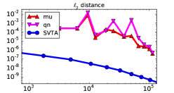
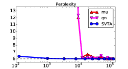
Figure 2: (top) $\ell_{2}$ distance between functions. (bottom) Perplexity on the test set. The $x$ axis denotes in both cases the number of parameters used by the approximation.

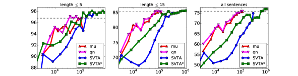
Figure 3: Parsing accuracy on the test set for different sentence lengths. The $x$-axis denote the number of parameters used by the approximation. The $y$-axis denotes bracketing accuracy.

For parsing we use minimum Bayes risk decoding, maximizing the sum of the marginals for the nonterminals in the grammar, essentially choosing the best tree topology given a string Goodman, (1996). The results for various length of sentences are shown in Figure 3, where we see that our method does not perform as well as the tensor decomposition methods in terms of parsing accuracy on long sentences. In this figure, we also plotted the results for a slight modification of our method (SVTA^∗) that is able to achieve competitive performances. The SVTA^∗ method gives more importance to long sentences in the minimization process. This is done by finding the highest constant $\gamma>0$ such that the function $f_{\gamma}:t\mapsto\gamma^{\mathrm{size}(t)}f(t)$ is still strongly convergent. This function is then approximated by a low-rank WTA computing $\hat{f}_{\gamma}$, and we let $\hat{f}:t\mapsto\gamma^{-\mathrm{size}(t)}\hat{f}_{\gamma}(t)$ (which is rational). In our experiment, we used $\gamma=2.4$. While the SVTA^∗ method improved the parsing accuracy, it had no significant repercussion on the $\ell_{2}$ and perplexity measures. We believe that the parsing accuracy of our method could be further improved. Seeking techniques that combines the benefits of SVTA and previous works is a promising direction.

6 Conclusion

We described a technique for approximate minimization of WTA, yielding a model smaller than the original one which retains good approximation properties. Our main algorithm relies on a singular value decomposition of an infinite Hankel matrix induced by the WTA. We provided theoretical guarantees on the error induced by our minimization method. Our experiments with real-world parsing data show that the minimized WTA, depending on the number of singular values used, approximates well the original WTA on three measures: perplexity, bracketing accuracy and $\ell_{2}$ distance of the tree weights. Our work has connections with spectral learning techniques for WTA, and exhibits similar properties as those algorithms; e.g. absence of local optima. In future work we plan to investigate the applications of our approach to the design and analysis of improved spectral learning algorithms for WTA.

Appendix A Proof of Theorem 2

Theorem.

Let $f:\mathfrak{T}\to\mathbb{R}$ be rational. If $\mathbf{H}_{f}=\mathbf{P}\mathbf{S}$ is a rank factorization, then there exists a minimal WTA $A$ computing $f$ such that $\mathbf{P}_{A}=\mathbf{P}$ and $\mathbf{S}_{A}=\mathbf{S}$.

Proof.

Let $n=\mathop{rank}(f)$. Let $B$ be an arbitrary minimal WTA computing $f$. Suppose $B$ induces the rank factorization $\mathbf{H}_{f}=\mathbf{P}^{\prime}\mathbf{S}^{\prime}$. Since the columns of both $\mathbf{P}$ and $\mathbf{P}^{\prime}$ are basis for the column-span of $\mathbf{H}_{f}$, there must exists a change of basis $\mathbf{Q}\in\mathbb{R}^{n\times n}$ between $\mathbf{P}$ and $\mathbf{P}^{\prime}$. That is, $\mathbf{Q}$ is an invertible matrix such that $\mathbf{P}^{\prime}\mathbf{Q}=\mathbf{P}$. Furthermore, since $\mathbf{P}^{\prime}\mathbf{S}^{\prime}=\mathbf{H}_{f}=\mathbf{P}\mathbf{S}=\mathbf{P}^{\prime}\mathbf{Q}\mathbf{S}$ and $\mathbf{P}^{\prime}$ has full column rank, we must have $\mathbf{S}^{\prime}=\mathbf{Q}\mathbf{S}$, or equivalently, $\mathbf{Q}^{-1}\mathbf{S}^{\prime}=\mathbf{S}$. Thus, we let $A=B^{\mathbf{Q}}$, which immediately verifies $f_{A}=f_{B}=f$. It remains to be shown that $A$ induces the rank factorization $\mathbf{H}_{f}=\mathbf{P}\mathbf{S}$. Note that when proving the equivalence $f_{A}=f_{B}$ we already showed $\mathbf{\boldsymbol{\omega}}_{A}(t)=\mathbf{Q}^{-1}\mathbf{\boldsymbol{\omega}}_{B}(t)$, which means we have $\mathbf{S}_{A}=\mathbf{Q}^{-1}\mathbf{S}^{\prime}=\mathbf{S}$. To show $\mathbf{P}_{A}=\mathbf{P}^{\prime}\mathbf{Q}$ we need to show that for any $c\in\mathfrak{C}$ we have $\mathbf{\boldsymbol{\alpha}}_{A}(c)^{\top}=\mathbf{\boldsymbol{\alpha}}_{B}(c)^{\top}\mathbf{Q}$. This will immediately follow if we show that $\mathbf{\boldsymbol{\Xi}}_{A}(c)=\mathbf{Q}^{-1}\mathbf{\boldsymbol{\Xi}}_{B}(c)\mathbf{Q}$. If we proceed by induction on $\mathrm{drop}(c)$, we see the case $c=\ast$ is immediate, and for $c=(c^{\prime},t)$ we get

$$\mathbf{\boldsymbol{\Xi}}_{A}((c^{\prime},t)) =(\mathbf{\boldsymbol{\mathcal{T}}}(\mathbf{Q}^{-\top},\mathbf{Q},\mathbf{Q}))(\mathbf{I},\mathbf{\boldsymbol{\Xi}}_{A}(c^{\prime}),\mathbf{\boldsymbol{\omega}}_{A}(t))$$

$$=(\mathbf{\boldsymbol{\mathcal{T}}}(\mathbf{Q}^{-\top},\mathbf{Q},\mathbf{Q}))(\mathbf{I},\mathbf{Q}^{-1}\mathbf{\boldsymbol{\Xi}}_{B}(c^{\prime})\mathbf{Q},\mathbf{Q}^{-1}\mathbf{\boldsymbol{\omega}}_{B}(t))$$

$$=\mathbf{\boldsymbol{\mathcal{T}}}(\mathbf{Q}^{-\top},\mathbf{\boldsymbol{\Xi}}_{B}(c^{\prime})\mathbf{Q},\mathbf{\boldsymbol{\omega}}_{B}(t))$$

$$=\mathbf{Q}^{-1}\mathbf{\boldsymbol{\mathcal{T}}}(\mathbf{I},\mathbf{\boldsymbol{\Xi}}_{B}(c^{\prime}),\mathbf{\boldsymbol{\omega}}_{B}(t))\mathbf{Q}\enspace.$$

Applying the same argument mutatis mutandis for $c=(t,c^{\prime})$ completes the proof. ∎

Appendix B Proof of Theorem 3

Theorem.

If $f:\mathfrak{T}_{\Sigma}\to\mathbb{R}$ is rational and strongly convergent, then $\mathbf{H}_{f}$ admits a singular value decomposition.

Proof.

The result will follow if we show that $\mathbf{H}_{f}$ is the matrix of a compact operator on a Hilbert space Conway, (1990). The main obstruction to this approach is that the rows and columns of $\mathbf{H}_{f}$ are indexed by different objects (trees vs. contexts). Thus, we will need to see $\mathbf{H}_{f}$ as an operator on a larger space that contains both these objects.

Recall we have $\mathfrak{T}_{\Sigma}\subset\mathfrak{T}_{\Sigma^{\prime}}$ and $\mathfrak{C}_{\Sigma}\subset\mathfrak{T}_{\Sigma^{\prime}}$. Given two functions $g,g^{\prime}:\mathfrak{T}_{\Sigma^{\prime}}\to\mathbb{R}$ we define their inner product to be $\left<g,g^{\prime}\right>=\sum_{t^{\prime}\in\mathfrak{T}_{\Sigma^{\prime}}}g(t^{\prime})g^{\prime}(t^{\prime})$. Let $\|g\|=\sqrt{|\left<g,g\right>|}$ be the induced norm and let $\mathbb{T}$ be the space of all functions $g:\mathfrak{T}_{\Sigma^{\prime}}\to\mathbb{R}$ such that $\|g\|<\infty$. Note that $\mathbb{T}$ with a Hilbert space, and that since $\mathfrak{T}_{\Sigma^{\prime}}$ is countable, it actually is a separable Hilbert space isomorphic to $\ell^{2}$, the spaces of infinite square summable sequences. Given set $\mathfrak{X}\subset\mathfrak{T}_{\Sigma^{\prime}}$ we define $\mathbb{T}(\mathfrak{X})=\{g\in\mathbb{T}\;|\;g(t^{\prime})=0,t^{\prime}\in\mathfrak{T}_{\Sigma^{\prime}}\setminus\mathfrak{X}\}$.

Now let $C_{f}:\mathbb{T}\to\mathbb{T}$ be the linear operator on $\mathbb{T}$ given by

$$(C_{f}g)(t^{\prime})=\begin{cases}\sum_{t\in\mathfrak{T}_{\Sigma}}f(t^{\prime}[t])g(t)&\text{if $t^{\prime}\in\mathfrak{C}_{\Sigma}$}\\ 0&\text{if $t^{\prime}\notin\mathfrak{C}_{\Sigma}$}\enspace.\end{cases}$$

Now note that by construction we have $\mathbb{T}(\mathfrak{T}_{\Sigma})\subseteq\mathrm{Ker}(C_{f})$ and $\mathrm{Im}(C_{f})\subseteq\mathbb{T}(\mathfrak{C}_{\Sigma})$. Hence, a simple calculation shows that given the decompositions $C_{f}:\mathbb{T}(\mathfrak{T}_{\Sigma})^{\bot}\oplus\mathbb{T}(\mathfrak{T}_{\Sigma})\to\mathbb{T}(\mathfrak{C}_{\Sigma})\oplus\mathbb{T}(\mathfrak{C}_{\Sigma})^{\bot}$, the matrix of $C_{f}$ is

$$\mathbf{C}_{f}=\left[\begin{array}[]{cc}\mathbf{H}_{f}&\mathbf{0}\\ \mathbf{0}&\mathbf{0}\end{array}\right]\enspace.$$

Thus, if $C_{f}$ is a compact operator, then $\mathbf{H}_{f}$ admits an SVD. Since $\mathbf{H}_{f}$ has finite rank, we only need to show that $C_{f}$ is a bounded operator.

Given $c\in\mathfrak{C}_{\Sigma}$ we define $f_{c}\in\mathbb{T}(\mathfrak{T}_{\Sigma})$ given by $f_{c}(t)=f(c[t])$ for $t\in\mathfrak{T}_{\Sigma}$. Now let $g\in\mathbb{T}$ with $\|g\|=1$ and recall $C_{f}$ is bounded if $\|C_{f}g\|<\infty$ for every $g\in\mathbb{T}$ with $\|g\|=1$. Indeed, because $f$ is strongly convergent we have:

$$\|C_{f}g\|^{2} =\sum_{t^{\prime}\in\mathfrak{T}_{\Sigma^{\prime}}}(C_{f}g)(t^{\prime})^{2}$$

$$=\sum_{c\in\mathfrak{C}_{\Sigma}}(C_{f}g)(c)^{2}$$

$$=\sum_{c\in\mathfrak{C}_{\Sigma}}\left(\sum_{t\in\mathfrak{T}_{\Sigma}}f(c[t])g(t)\right)^{2}$$

$$=\sum_{c\in\mathfrak{C}_{\Sigma}}\left<f_{c},g\right>^{2}$$

$$\leq\|g\|^{2}\sum_{c\in\mathfrak{C}_{\Sigma}}\|f_{c}\|^{2}$$

$$=\sum_{c\in\mathfrak{C}_{\Sigma}}\sum_{t^{\prime}\in\mathfrak{T}_{\Sigma^{\prime}}}f_{c}(t^{\prime})^{2}$$

$$=\sum_{c\in\mathfrak{C}_{\Sigma}}\sum_{t\in\mathfrak{T}_{\Sigma}}f(c[t])^{2}$$

$$=\sum_{t\in\mathfrak{T}_{\Sigma}}|t|f(t)^{2}$$

$$\leq\sup_{t\in\mathfrak{T}_{\Sigma}}|f(t)|\cdot\sum_{t\in\mathfrak{T}_{\Sigma}}|t||f(t)|<\infty\enspace,$$

where we used the Cauchy–Schwarz inequality, and the fact that $\sup_{t\in\mathfrak{T}_{\Sigma}}|f(t)|$ is bounded when $f$ is strongly convergent. ∎

Appendix C Proof of Theorem 4

Theorem.

Let $F:\mathbb{R}^{n^{2}}\to\mathbb{R}^{n^{2}}$ be the mapping defined by $F(\mathbf{v})=\mathbf{\boldsymbol{\mathcal{T}}}^{\otimes}(\mathbf{I},\mathbf{v},\mathbf{v})+\sum_{\sigma\in\Sigma}\mathbf{\boldsymbol{\omega}}^{\otimes}_{\sigma}$. Then the following hold:

• $\mathbf{s}$ is a fixed-point of $F$; i.e. $F(\mathbf{s})=\mathbf{s}$.

• $\mathbf{0}$ is in the basin of attraction of $\mathbf{s}$; i.e. $\lim_{k\to\infty}F^{k}(\mathbf{0})=\mathbf{s}$.

• The iteration defined by $\mathbf{s}_{0}=\mathbf{0}$ and $\mathbf{s}_{k+1}=F(\mathbf{s}_{k})$ converges linearly to $\mathbf{s}$; i.e. there exists $0<\rho<1$ such that $\|\mathbf{s}_{k}-\mathbf{s}\|_{2}\leq\mathcal{O}(\rho^{k})$.

Proof.

(i) We have $\mathbf{\boldsymbol{\mathcal{T}}}^{\otimes}(\mathbf{I},\mathbf{s},\mathbf{s})=\sum_{t,t^{\prime}\in\mathfrak{T}}\mathbf{\boldsymbol{\mathcal{T}}}^{\otimes}(\mathbf{I},\mathbf{\boldsymbol{\omega}}^{\otimes}(t),\mathbf{\boldsymbol{\omega}}^{\otimes}(t^{\prime}))=\sum_{t,t^{\prime}\in\mathfrak{T}}\mathbf{\boldsymbol{\omega}}^{\otimes}((t,t^{\prime}))=\sum_{t\in\mathfrak{T}^{\geq 1}}\mathbf{\boldsymbol{\omega}}^{\otimes}(t)$ where $\mathfrak{T}^{\geq 1}$ is the set of trees of depth at least one. Hence $F(\mathbf{s})=\sum_{t\in\mathfrak{T}^{\geq 1}}\mathbf{\boldsymbol{\omega}}^{\otimes}(t)+\sum_{\sigma\in\Sigma}\mathbf{\boldsymbol{\omega}}^{\otimes}_{\sigma}=\mathbf{s}$.

(ii) Let $\mathfrak{T}^{\leq k}$ denote the set of all trees with depth at most $k$. We prove by induction on $k$ that $F^{k}(\mathbf{0})=\sum_{t\in\mathfrak{T}^{\leq k}}\mathbf{\boldsymbol{\omega}}^{\otimes}(t)$, which implies that $\lim_{k\to\infty}F^{k}(\mathbf{0})=\mathbf{s}$. This is straightforward for $k=0$. Assuming it is true for all naturals up to $k-1$, we have

$$F^{k}(\mathbf{0}) =\mathbf{\boldsymbol{\mathcal{T}}}^{\otimes}(\mathbf{I},F^{k-1}(\mathbf{0}),F^{k-1}(\mathbf{0}))+\sum_{\sigma\in\Sigma}\mathbf{\boldsymbol{\omega}}^{\otimes}_{\sigma}$$

$$=\sum_{t,t^{\prime}\in\mathfrak{T}^{\leq k-1}}\mathbf{\boldsymbol{\mathcal{T}}}^{\otimes}(\mathbf{I},\mathbf{\boldsymbol{\omega}}^{\otimes}(t),\mathbf{\boldsymbol{\omega}}^{\otimes}(t^{\prime}))+\sum_{\sigma\in\Sigma}\mathbf{\boldsymbol{\omega}}^{\otimes}_{\sigma}$$

$$=\sum_{t,t^{\prime}\in\mathfrak{T}^{\leq k-1}}\mathbf{\boldsymbol{\omega}}^{\otimes}((t,t^{\prime}))+\sum_{\sigma\in\Sigma}\mathbf{\boldsymbol{\omega}}^{\otimes}_{\sigma}$$

$$=\sum_{t\in\mathfrak{T}^{\leq k}}\mathbf{\boldsymbol{\omega}}^{\otimes}(t)\enspace.$$

(iii) Let $\mathbf{E}$ be the Jacobian of $F$ around $\mathbf{s}$, we show that the spectral radius $\rho(\mathbf{E})$ of $\mathbf{E}$ is less than one, which implies the result by Ostrowski’s theorem (see (Ortega,, 1990, Theorem 8.1.7)).

Since $A$ is minimal, there exists trees $t_{1},\cdots,t_{n}\in\mathfrak{T}$ and contexts $c_{1},\cdots,c_{n}\in\mathfrak{C}$ such that both $\{\mathbf{\boldsymbol{\omega}}(t_{i})\}_{i\in[n]}$ and $\{\mathbf{\boldsymbol{\alpha}}(c_{i})\}_{i\in[n]}$ are sets of linear independent vectors in $\mathbb{R}^{n}$ Bailly et al., (2010). Therefore, the sets $\{\mathbf{\boldsymbol{\omega}}(t_{i})\otimes\mathbf{\boldsymbol{\omega}}(t_{j})\}_{i,j\in[n]}$ and $\{\mathbf{\boldsymbol{\alpha}}(c_{i})\otimes\mathbf{\boldsymbol{\alpha}}(c_{j})\}_{i,j\in[n]}$ are sets of linear independent vectors in $\mathbb{R}^{n^{2}}$. Let $\mathbf{v}\in\mathbb{R}^{n^{2}}$ be an eigenvector of $\mathbf{E}$ with eigenvalue $\lambda\neq 0$, and let $\mathbf{v}=\sum_{i,j\in[n]}\beta_{i,j}(\mathbf{\boldsymbol{\omega}}(t_{i})\otimes\mathbf{\boldsymbol{\omega}}(t_{j}))$ be its expression in terms of the basis given by $\{\mathbf{\boldsymbol{\omega}}(t_{i})\otimes\mathbf{\boldsymbol{\omega}}(t_{j})\}$. For any vector $\mathbf{u}\in\{\mathbf{\boldsymbol{\alpha}}(c_{i})\otimes\mathbf{\boldsymbol{\alpha}}(c_{j})\}$ we have

$$\lim_{k\to\infty}\mathbf{u}^{\top}\mathbf{E}^{k}\mathbf{v}\leq\lim_{k\to\infty}|\mathbf{u}^{\top}\mathbf{E}^{k}\mathbf{v}|\leq\sum_{i,j\in[n]}|\beta_{i,j}|\lim_{k\to\infty}|\mathbf{u}^{\top}\mathbf{E}^{k}(\mathbf{\boldsymbol{\omega}}(t_{i})\otimes\mathbf{\boldsymbol{\omega}}(t_{j}))|=0\enspace,$$

where we used Lemma 2 in the last step. Since this is true for any vector $\mathbf{u}$ in the basis $\{\mathbf{\boldsymbol{\alpha}}(c_{i})\otimes\mathbf{\boldsymbol{\alpha}}(c_{j})\}$, we have $\lim_{k\to\infty}\mathbf{E}^{k}\mathbf{v}=\lim_{k\to\infty}|\lambda|^{k}\mathbf{v}=\mathbf{0}$, hence $|\lambda|<1$. This reasoning holds for any eigenvalue of $\mathbf{E}$, hence $\rho(\mathbf{E})<1$. ∎

Lemma 2.

Let $A=\langle\mathbf{\boldsymbol{\alpha}},\mathbf{\boldsymbol{\mathcal{T}}},\{\mathbf{\boldsymbol{\omega}}_{\sigma}\}\rangle$ be a minimal WTA of dimension $n$ computing the strongly convergent function $f$, and let $\mathbf{E}\in\mathbb{R}^{n^{2}\times n^{2}}$ be the Jacobian around $\mathbf{s}=\sum_{t\in\mathfrak{T}}\mathbf{\boldsymbol{\omega}}(t)\otimes\mathbf{\boldsymbol{\omega}}(t)$ of the mapping $F:\mathbf{v}\to\mathbf{\boldsymbol{\mathcal{T}}}^{\otimes}(\mathbf{I},\mathbf{v},\mathbf{v})+\sum_{\sigma\in\Sigma}\mathbf{\boldsymbol{\omega}}^{\otimes}_{\sigma}$. Then for any $c_{1},c_{2}\in\mathfrak{C}$ and any $t_{1},t_{2}\in\mathfrak{T}$ we have $\lim_{k\to\infty}|(\mathbf{\boldsymbol{\alpha}}(c_{1})\otimes\mathbf{\boldsymbol{\alpha}}(c_{2}))^{\top}\mathbf{E}^{k}(\mathbf{\boldsymbol{\omega}}(t_{1})\otimes\mathbf{\boldsymbol{\omega}}(t_{2}))|=0$.

Proof.

Let $\mathbf{\boldsymbol{\Xi}}^{\otimes}:\mathfrak{C}\to\mathbb{R}^{n^{2}\times n^{2}}$ be the context mapping associated with the WTA $A^{\otimes}$; i.e. $\mathbf{\boldsymbol{\Xi}}^{\otimes}=\mathbf{\boldsymbol{\Xi}}_{A^{\otimes}}$. We start by proving by induction on $\mathrm{drop}(c)$ that $\mathbf{\boldsymbol{\Xi}}^{\otimes}(c)=\mathbf{\boldsymbol{\Xi}}(c)\otimes\mathbf{\boldsymbol{\Xi}}(c)$ for all $c\in\mathfrak{C}$. Let $\mathfrak{C}^{d}$ denote the set of contexts $c\in\mathfrak{C}$ with $\mathrm{drop}(c)=d$. The statement is trivial for $c\in\mathfrak{C}^{0}$. Assume the statement is true for all naturals up to $d-1$ and let $c=(t,c^{\prime})\in\mathfrak{C}^{d}$ for some $t\in\mathfrak{T}$ and $c^{\prime}\in\mathfrak{C}^{d-1}$. Then using our inductive hypothesis we have that

$$\mathbf{\boldsymbol{\Xi}}^{\otimes}(c) =\mathbf{\boldsymbol{\mathcal{T}}}^{\otimes}(\mathbf{I}_{n^{2}},\mathbf{\boldsymbol{\omega}}(t)\otimes\mathbf{\boldsymbol{\omega}}(t),\mathbf{\boldsymbol{\Xi}}(c^{\prime})\otimes\mathbf{\boldsymbol{\Xi}}(c^{\prime}))$$

$$=\mathbf{\boldsymbol{\mathcal{T}}}(\mathbf{I}_{n},\mathbf{\boldsymbol{\omega}}(t),\mathbf{\boldsymbol{\Xi}}(c^{\prime}))\otimes\mathbf{\boldsymbol{\mathcal{T}}}(\mathbf{I}_{n},\mathbf{\boldsymbol{\omega}}(t),\mathbf{\boldsymbol{\Xi}}(c^{\prime}))$$

$$=\mathbf{\boldsymbol{\Xi}}(c)\otimes\mathbf{\boldsymbol{\Xi}}(c)\enspace.$$

The case $c=(c^{\prime},t)$ follows from an identical argument.

Next we use the multi-linearity of $F$ to expand $F(\mathbf{s}+\mathbf{h})$ for a vector $\mathbf{h}\in\mathbb{R}^{n^{2}}$. Keeping the terms that are linear in $\mathbf{h}$ we obtain that $\mathbf{E}=\mathbf{\boldsymbol{\mathcal{T}}}^{\otimes}(\mathbf{I},\mathbf{s},\mathbf{I})+\mathbf{\boldsymbol{\mathcal{T}}}^{\otimes}(\mathbf{I},\mathbf{I},\mathbf{s})$. It follows that $\mathbf{E}=\sum_{c\in\mathfrak{C}^{1}}\mathbf{\boldsymbol{\Xi}}^{\otimes}(c)$, and it can be shown by induction on $k$ that $\mathbf{E}^{k}=\sum_{c\in\mathfrak{C}^{k}}\mathbf{\boldsymbol{\Xi}}^{\otimes}(c)$.

Writing $d_{c}=\min(\mathrm{drop}(c_{1}),\mathrm{drop}(c_{2}))$ and $d_{t}=\min(0pt{t_{1}},0pt{t_{2}})$, we can see that

$$\left|(\mathbf{\boldsymbol{\alpha}}(c_{1})\otimes\mathbf{\boldsymbol{\alpha}}(c_{2}))^{\top}\mathbf{E}^{k}(\mathbf{\boldsymbol{\omega}}(t_{1})\otimes\mathbf{\boldsymbol{\omega}}(t_{2}))\right| =\left|\sum_{c\in\mathfrak{C}^{k}}(\mathbf{\boldsymbol{\alpha}}(c_{1})\otimes\mathbf{\boldsymbol{\alpha}}(c_{2}))^{\top}\mathbf{\boldsymbol{\Xi}}^{\otimes}(c)(\mathbf{\boldsymbol{\omega}}(t_{1})\otimes\mathbf{\boldsymbol{\omega}}(t_{2}))\right|$$

$$=\left|\sum_{c\in\mathfrak{C}^{k}}(\mathbf{\boldsymbol{\alpha}}(c_{1})^{\top}\mathbf{\boldsymbol{\Xi}}(c)\mathbf{\boldsymbol{\omega}}(t_{1}))\cdot(\mathbf{\boldsymbol{\alpha}}(c_{2})^{\top}\mathbf{\boldsymbol{\Xi}}(c)\mathbf{\boldsymbol{\omega}}(t_{2}))\right|$$

$$=\left|\sum_{c\in\mathfrak{C}^{k}}f(c_{1}[c[t_{1}]])f(c_{2}[c[t_{2}]])\right|$$

$$\leq\left(\sum_{c\in\mathfrak{C}^{k}}|f(c_{1}[c[t_{1}]])|\right)\left(\sum_{c\in\mathfrak{C}^{k}}|f(c_{2}[c[t_{2}]])|\right)$$

$$\leq\left(\sum_{t\in\mathfrak{T}^{\geq d_{c}+d_{t}+k}}|t||f(t)|\right)^{2}\enspace,$$

which tends to $0$ with $k\to\infty$ since $f$ is strongly convergent. To prove the last inequality, check that any tree of the form $t^{\prime}=c[c^{\prime}[t]]$ satisfies $0pt{t^{\prime}}\geq\mathrm{drop}(c)+\mathrm{drop}(c^{\prime})+0pt{t}$, and that for fixed $c\in\mathfrak{C}$ and $t,t^{\prime}\in\mathfrak{T}$ we have $|\{c^{\prime}\in\mathfrak{C}:c[c^{\prime}[t]]=t^{\prime}\}|\leq|t^{\prime}|$ (indeed, a factorization $t^{\prime}=c[c^{\prime}[t]]$ is fixed once the root of $t$ is chosen in $t^{\prime}$, which can be done in at most $|t^{\prime}|$ different ways). ∎

Appendix D Proof of Theorem 5

Theorem.

There exists $0<\rho<1$ such that after $k$ iterations in Algorithm 2, the approximations $\hat{\mathbf{G}}_{\mathfrak{C}}$ and $\hat{\mathbf{G}}_{\mathfrak{T}}$ satisfy $\|\mathbf{G}_{\mathfrak{C}}-\hat{\mathbf{G}}_{\mathfrak{C}}\|_{F}\leq\mathcal{O}(\rho^{k})$ and $\|\mathbf{G}_{\mathfrak{T}}-\hat{\mathbf{G}}_{\mathfrak{T}}\|_{F}\leq\mathcal{O}(\rho^{k})$.

Proof.

The result for the Gram matrix $\mathbf{G}_{\mathfrak{T}}$ directly follows from Theorem 4. We now show how the error in the approximation of $\mathbf{G}_{\mathfrak{T}}=\operatorname*{reshape}(\mathbf{s},n\times n)$ affects the approximation of $\mathbf{q}=(\mathbf{\boldsymbol{\alpha}}^{\otimes})^{\top}(\mathbf{I}-\mathbf{E})^{-1}=\operatorname*{vec}(\mathbf{G}_{\mathfrak{C}})$. Let $\hat{\mathbf{s}}\in\mathbb{R}^{n}$ be such that $\|\mathbf{s}-\hat{\mathbf{s}}\|\leq\varepsilon$, let $\hat{\mathbf{E}}=\mathbf{\boldsymbol{\mathcal{T}}}^{\otimes}(\mathbf{I},\hat{\mathbf{s}},\mathbf{I})+\mathbf{\boldsymbol{\mathcal{T}}}^{\otimes}(\mathbf{I},\mathbf{I},\hat{\mathbf{s}})$ and let $\mathbf{q}=(\mathbf{\boldsymbol{\alpha}}^{\otimes})^{\top}(\mathbf{I}-\hat{\mathbf{E}})^{-1}$. We first bound the distance between $\mathbf{E}$ and $\hat{\mathbf{E}}$. We have

$$\|\mathbf{E}-\hat{\mathbf{E}}\|_{F} =\|\mathbf{\boldsymbol{\mathcal{T}}}^{\otimes}(\mathbf{I},\mathbf{s}-\hat{\mathbf{s}},\mathbf{I})+\mathbf{\boldsymbol{\mathcal{T}}}^{\otimes}(\mathbf{I},\mathbf{I},\mathbf{s}-\hat{\mathbf{s}})\|_{F}$$

$$\leq 2\|\mathbf{\boldsymbol{\mathcal{T}}}^{\otimes}\|_{F}\|\mathbf{s}-\hat{\mathbf{s}}\|$$

$$=\mathcal{O}(\varepsilon)\enspace,$$

where we used the bounds $\|\mathbf{\boldsymbol{\mathcal{T}}}(\mathbf{I},\mathbf{I},\mathbf{v})\|_{F}\leq\|\mathbf{\boldsymbol{\mathcal{T}}}\|_{F}\|\mathbf{v}\|$ and $\|\mathbf{\boldsymbol{\mathcal{T}}}(\mathbf{I},\mathbf{v},\mathbf{I})\|_{F}\leq\|\mathbf{\boldsymbol{\mathcal{T}}}\|_{F}\|\mathbf{v}\|$.

Let $\delta=\|\mathbf{E}-\hat{\mathbf{E}}\|$ and let $\sigma$ be the smallest nonzero eigenvalue of the matrix $\mathbf{I}-\mathbf{E}$. It follows from (El Ghaoui,, 2002, Equation (7.2)) that if $\delta<\sigma$ then $\|(\mathbf{I}-\mathbf{E})^{-1}-(\mathbf{I}-\hat{\mathbf{E}})^{-1}\|\leq\delta/(\sigma(\sigma-\delta))$. Since $\delta=\mathcal{O}(\varepsilon)$ from our previous bound, the condition $\delta\leq\sigma/2$ will be eventually satisfied as $\varepsilon\to 0$, in which case we can conclude that

$$\|\mathbf{G}_{\mathfrak{C}}-\hat{\mathbf{G}}_{\mathfrak{C}}\|_{F} =\|\mathbf{q}-\hat{\mathbf{q}}\|$$

$$\leq\|(\mathbf{I}-\mathbf{E})^{-1}-(\mathbf{I}-\hat{\mathbf{E}})^{-1}\|\|\mathbf{\boldsymbol{\alpha}}^{\otimes}\|$$

$$\leq\frac{2\delta}{\sigma^{2}}\|\mathbf{\boldsymbol{\alpha}}^{\otimes}\|$$

$$=\mathcal{O}(\varepsilon)\enspace.$$

∎

Appendix E Proof of Theorem 6

Let $A=\langle\mathbf{\boldsymbol{\alpha}},\mathbf{\boldsymbol{\mathcal{T}}},\{\mathbf{\boldsymbol{\omega}}_{\sigma}\}_{\sigma\in\Sigma}\rangle$ be a SVTA with $n$ states realizing a function $f$ and let $\mathfrak{s}_{1}\geq\mathfrak{s}_{2}\geq\cdots\geq\mathfrak{s}_{n}$ be the singular values of the Hankel matrix $\mathbf{H}_{f}$.

Theorem 6 relies on the following lemma, which explores the consequences that the fixed-point equations used to compute $\mathbf{G}_{\mathfrak{T}}$ and $\mathbf{G}_{\mathfrak{C}}$ have for an SVTA.

Lemma 3.

For all $i\in[n]$, the following hold:

1. $\mathfrak{s}_{i}=\sum_{\sigma\in\Sigma}\mathbf{\boldsymbol{\omega}}_{\sigma}(i)^{2}+\sum_{j,k=1}^{n}\mathbf{\boldsymbol{\mathcal{T}}}(i,j,k)^{2}\mathfrak{s}_{j}\mathfrak{s}_{k}\enspace,$

2. $\mathfrak{s}_{i}=\mathbf{\boldsymbol{\alpha}}(j)^{2}+\sum_{j,k=1}^{n}(\mathbf{\boldsymbol{\mathcal{T}}}(j,i,k)^{2}+\mathbf{\boldsymbol{\mathcal{T}}}(j,k,i)^{2})\mathfrak{s}_{j}\mathfrak{s}_{k}\enspace.$

Proof.

Let $\mathbf{G}_{\mathfrak{T}}$ and $\mathbf{G}_{\mathfrak{C}}$ be the Gram matrices associated with the rank factorization of $\mathbf{H}_{f}$. Since $A$ is a SVTA we have $\mathbf{G}_{\mathfrak{T}}=\mathbf{G}_{\mathfrak{C}}=\mathbf{D}$ where $\mathbf{D}=\mathop{diag}(\mathfrak{s}_{1},\cdots,\mathfrak{s}_{n})$ is a diagonal matrix with the Hankel singular values on the diagonal. The first equality then follows from the following fixed point characterization of $\mathbf{G}_{\mathfrak{T}}$:

$$\mathbf{G}_{\mathfrak{T}} =\sum_{t\in\mathfrak{T}}\mathbf{\boldsymbol{\omega}}(t)\mathbf{\boldsymbol{\omega}}(t)^{\top}$$

$$=\sum_{\sigma\in\Sigma}\mathbf{\boldsymbol{\omega}}_{\sigma}\mathbf{\boldsymbol{\omega}}_{\sigma}^{\top}$$

$$+\sum_{t_{1},t_{2}\in\mathfrak{T}}\mathbf{\boldsymbol{\mathcal{T}}}(\mathbf{I},\mathbf{\boldsymbol{\omega}}(t_{1}),\mathbf{\boldsymbol{\omega}}(t_{2}))\mathbf{\boldsymbol{\mathcal{T}}}(\mathbf{I},\mathbf{\boldsymbol{\omega}}(t_{1}),\mathbf{\boldsymbol{\omega}}(t_{2}))^{\top}$$

$$=\sum_{\sigma\in\Sigma}\mathbf{\boldsymbol{\omega}}_{\sigma}\mathbf{\boldsymbol{\omega}}_{\sigma}^{\top}+\mathbf{T}_{(1)}(\mathbf{G}_{\mathfrak{T}}\otimes\mathbf{G}_{\mathfrak{T}})\mathbf{T}_{(1)}^{\top}\enspace,$$

(where $\mathbf{T}_{(}i)$ denotes the matricization of the tensor $\mathbf{\boldsymbol{\mathcal{T}}}$ along the $i$th mode). The second equality follows from the following fixed point characterization of $\mathbf{G}_{\mathfrak{C}}$:

$$\mathbf{G}_{\mathfrak{C}} =\sum_{c\in\mathfrak{C}}\mathbf{\boldsymbol{\alpha}}(c)\mathbf{\boldsymbol{\alpha}}(c)^{\top}$$

$$=\mathbf{\boldsymbol{\alpha}}\mathbf{\boldsymbol{\alpha}}^{\top}$$

$$+\sum_{c\in\mathfrak{C},t\in\mathfrak{T}}\mathbf{\boldsymbol{\mathcal{T}}}(\mathbf{\boldsymbol{\alpha}}(c),\mathbf{\boldsymbol{\omega}}(t),\mathbf{I})\mathbf{\boldsymbol{\mathcal{T}}}(\mathbf{\boldsymbol{\alpha}}(c),\mathbf{\boldsymbol{\omega}}(t),\mathbf{I})^{\top}$$

$$+\sum_{c\in\mathfrak{C},t\in\mathfrak{T}}\mathbf{\boldsymbol{\mathcal{T}}}(\mathbf{\boldsymbol{\alpha}}(c),\mathbf{I},\mathbf{\boldsymbol{\omega}}(t))\mathbf{\boldsymbol{\mathcal{T}}}(\mathbf{\boldsymbol{\alpha}}(c),\mathbf{I},\mathbf{\boldsymbol{\omega}}(t))^{\top}$$

$$=\mathbf{\boldsymbol{\alpha}}\mathbf{\boldsymbol{\alpha}}^{\top}$$

$$+\mathbf{T}_{(2)}(\mathbf{G}_{\mathfrak{C}}\otimes\mathbf{G}_{\mathfrak{T}})\mathbf{T}_{(2)}^{\top}$$

$$+\mathbf{T}_{(3)}(\mathbf{G}_{\mathfrak{C}}\otimes\mathbf{G}_{\mathfrak{T}})\mathbf{T}_{(3)}^{\top}\enspace.$$

∎

Theorem.

For any $t\in\mathfrak{T}$, $c\in\mathfrak{C}$ and $i,j,k\in[n]$ the following hold:

• $|\mathbf{\boldsymbol{\omega}}(t)_{i}|\leq\sqrt{\mathfrak{s}_{i}}$ ,

• $|\mathbf{\boldsymbol{\alpha}}(c)_{i}|\leq\sqrt{\mathfrak{s}_{i}}$ , and

• $|\mathbf{\boldsymbol{\mathcal{T}}}(i,j,k)|\leq\min\{\frac{\sqrt{\mathfrak{s}_{i}}}{\sqrt{\mathfrak{s}_{j}}\sqrt{\mathfrak{s}_{k}}},\frac{\sqrt{\mathfrak{s}_{j}}}{\sqrt{\mathfrak{s}_{i}}\sqrt{\mathfrak{s}_{k}}},\frac{\sqrt{\mathfrak{s}_{k}}}{\sqrt{\mathfrak{s}_{i}}\sqrt{\mathfrak{s}_{j}}}\}$.

Proof.

The third point is a direct consequence of the previous Lemma. For the first point, let $\mathbf{UDV}^{\top}$ be the SVD of $\mathbf{H}_{f}$. Since $A$ is a SVTA we have

$$\mathbf{\boldsymbol{\omega}}(t)_{i}^{2}=(\mathbf{D}^{1/2}\mathbf{V}^{\top})_{i,t}^{2}=\mathfrak{s}_{i}\mathbf{V}(t,i)^{2}$$

and since the rows of $\mathbf{V}$ are orthonormal we have $\mathbf{V}(t,i)^{2}\leq 1$.

The inequality for contexts is proved similarly by reasoning on the rows of $\mathbf{UD}^{1/2}$. ∎

Appendix F Proof of Theorem 7

To prove Theorem 7, we will show how the computation of a WTA on a give tree $t$ can be seen as an inner product between two tensors, one which is a function of the topology of the tree, and one which is a function of the labeling of its leafs (Proposition 1). We will then show a fundamental relation between the components of the first tensor and the singular values of the Hankel matrix when the WTA is in SVTA normal form (Proposition 2); this proposition will allow us to show Lemma 4 that bounds the difference between components of this first tensor for the original SVTA and its truncation. We will finally use this lemma to bound the absolute error introduced by the truncation of an SVTA (Propositions 3 and 4).

We first introduce another kind of contexts than the one introduced in Section 2, where every leaf of a binary tree is labeled by the special symbol $*$ (which still acts as a place holder). Let $\mathfrak{B}$ be the set of binary trees on the one-letter alphabet $\{*\}$. We will call a tree $b\in\mathfrak{B}$ a multicontext. For any integer $M\geq 1$ we let

$$\mathfrak{B}_{M}=\{b\in\mathfrak{B}:|\langle b\rangle|=M\}$$

be the subset of multicontexts with $M$ leaves (equivalently, $\mathfrak{B}_{M}$ is the subset of multicontexts of size $M-1$). Given a word $w=w_{1}\cdots w_{M}\in\Sigma^{*}$ and a multicontext $b\in\mathfrak{B}_{M}$, we denote by $b[w_{1},\cdots,w_{M}]\in\mathfrak{T}_{\Sigma}$ the tree obtained by replacing the $i$th occurrence of $*$ in $b$ by $w_{i}$ for $i\in[M]$. Let $b\in\mathfrak{B}_{M}$, for any integer $m\in[M]$ we denote by $b\llbracket m\rrbracket\in\mathfrak{B}_{M+1}$ the multicontext obtained by replacing the $m$th occurence of $*$ in $b$ by the tree $(*,*)$. Let $M>1$, it is easy to check that for any $b^{\prime}\in\mathfrak{B}_{M}$, there exist $b\in\mathfrak{B}_{M-1}$ and $m\in[M-1]$ satisfying $b^{\prime}=b\llbracket m\rrbracket$. See Figure 4 for some illustrative examples.

Figure 4: A multicontext $b=((*,*),*)\in\mathfrak{B}_{3}$, the tree $b[e,g,f]\in\mathfrak{T}$ and the multicontext $b\llbracket 2\rrbracket\in\mathfrak{B}_{4}$.

We now show how the computation of a WTA on a given tree with $M$ leaves can be seen as an inner product between two $M$th order tensors: the first one depends on the topology of the tree, while the second one depends on the labeling of its leaves. Let $A=\langle\mathbf{\boldsymbol{\alpha}},\mathbf{\boldsymbol{\mathcal{T}}},\{\mathbf{\boldsymbol{\omega}}_{\sigma}\}_{\sigma\in\Sigma}\rangle$ be a WTA with $n$ states computing a function $f$. Given a multicontext $b\in\mathfrak{B}_{M}$, we denote by $\mathbf{\boldsymbol{\beta}}_{A}(b)\in\bigotimes_{i=1}^{M}\mathbb{R}^{n}$ the $M$th order tensor inductively defined by $\mathbf{\boldsymbol{\beta}}_{A}(*)=\mathbf{\boldsymbol{\alpha}}$ and

$$\mathbf{\boldsymbol{\beta}}_{A}(b\llbracket m\rrbracket)_{i_{1}\cdots i_{M}}=\sum_{k=1}^{n}\mathbf{\boldsymbol{\beta}}_{A}(b)_{i_{1}\cdots i_{m-1}ki_{m+2}\cdots i_{M}}\mathbf{\boldsymbol{\mathcal{T}}}_{ki_{m}i_{m+1}}$$

for any $b\in\mathfrak{B}_{M-1}$, $m\in[M-1]$ and $i_{1},\cdots,i_{M}\in[n]$ (i.e. $\mathbf{\boldsymbol{\beta}}_{A}(b\llbracket m\rrbracket)$ is the contraction of $\mathbf{\boldsymbol{\beta}}_{A}(b)$ along the $m$th mode and $\mathbf{\boldsymbol{\mathcal{T}}}$ along the first mode). Given a word $w=w_{1}\cdots w_{M}\in\Sigma^{*}$, we let $\mathbf{\boldsymbol{\psi}}_{A}(w)\in\bigotimes_{i=1}^{M}\mathbb{R}^{n}$ be the $M$th order tensor defined by

$$\mathbf{\boldsymbol{\psi}}_{A}(w)_{i_{1}\cdots i_{M}}=\mathbf{\boldsymbol{\omega}}(w_{1})_{i_{1}}\mathbf{\boldsymbol{\omega}}(w_{2})_{i_{2}}\cdots\mathbf{\boldsymbol{\omega}}(w_{M})_{i_{M}}=\prod_{m=1}^{M}\mathbf{\boldsymbol{\omega}}(w_{m})_{i_{m}}$$

for $i_{1},\cdots,i_{M}\in[n]$ (i.e. $\mathbf{\boldsymbol{\psi}}_{A}(w)$ is the tensor product of the $\mathbf{\boldsymbol{\omega}}(w_{i})$’s). We will simply write $\mathbf{\boldsymbol{\beta}}$ and $\mathbf{\boldsymbol{\psi}}$ when the automaton is clear from context.

Proposition 1.

For any multicontext $b\in\mathfrak{B}_{M}$ and any word $w=w_{1}\cdots w_{M}\in\Sigma^{*}$ we have

$$f(b[w_{1},\cdots,w_{M}])=\langle\mathbf{\boldsymbol{\beta}}(b),\mathbf{\boldsymbol{\psi}}(w)\rangle\enspace,$$

where the inner product between two $M$th order tensors $\mathbf{\boldsymbol{\mathcal{U}}}$ and $\mathbf{\boldsymbol{\mathcal{V}}}$ is defined by $\langle\mathbf{\boldsymbol{\mathcal{U}}},\mathbf{\boldsymbol{\mathcal{V}}}\rangle=\sum_{i_{1}\cdots i_{M}}\mathbf{\boldsymbol{\mathcal{U}}}(i_{1},\cdots,i_{M})\mathbf{\boldsymbol{\mathcal{V}}}(i_{1},\cdots,i_{M})$.

Sketch of proof.

Let $b\in\mathfrak{B}_{M}$ and $w=w_{1}\cdots w_{M}\in\Sigma^{*}$. Let $b_{1}\in\mathfrak{B}_{M-1}$ and $m\in[M-1]$ be such that $b=b_{1}\llbracket m\rrbracket$. In order to lighten the notations and without loss of generality we assume that $m=1$. One can check that

$$\langle\mathbf{\boldsymbol{\beta}}(b),\mathbf{\boldsymbol{\psi}}(w)\rangle= \mathbf{\boldsymbol{\beta}}(b)(\mathbf{\boldsymbol{\omega}}_{w_{1}},\cdots,\mathbf{\boldsymbol{\omega}}_{w_{M}})$$

$$= \mathbf{\boldsymbol{\beta}}(b_{1}\llbracket 1\rrbracket)(\mathbf{\boldsymbol{\omega}}_{w_{1}},\cdots,\mathbf{\boldsymbol{\omega}}_{w_{M}})$$

$$= \mathbf{\boldsymbol{\beta}}(b_{1})(\mathbf{\boldsymbol{\omega}}((w_{1},w_{2})),\mathbf{\boldsymbol{\omega}}_{w_{3}},\cdots,\mathbf{\boldsymbol{\omega}}_{w_{M}})\enspace.$$

The same reasoning can now be applied to $b_{1}$. Assume for example that $b_{1}=b_{2}\llbracket 1\rrbracket$ for some $b_{2}\in\mathfrak{B}_{M-2}$, we would have

$$\langle\mathbf{\boldsymbol{\beta}}(b),\mathbf{\boldsymbol{\psi}}(w)\rangle =\mathbf{\boldsymbol{\beta}}(b_{1})(\mathbf{\boldsymbol{\omega}}((w_{1},w_{2})),\mathbf{\boldsymbol{\omega}}_{w_{3}},\cdots,\mathbf{\boldsymbol{\omega}}_{w_{M}})$$

$$=\mathbf{\boldsymbol{\beta}}(b_{2}\llbracket 1\rrbracket)(\mathbf{\boldsymbol{\omega}}((w_{1},w_{2})),\mathbf{\boldsymbol{\omega}}_{w_{3}},\cdots,\mathbf{\boldsymbol{\omega}}_{w_{M}})$$

$$=\mathbf{\boldsymbol{\beta}}(b_{2})(\mathbf{\boldsymbol{\omega}}(((w_{1},w_{2}),w_{3})),\mathbf{\boldsymbol{\omega}}_{w_{4}},\cdots,\mathbf{\boldsymbol{\omega}}_{w_{M}})\enspace.$$

By applying the same argument again and again we will eventually obtain

$$\langle\mathbf{\boldsymbol{\beta}}(b),\mathbf{\boldsymbol{\psi}}(w)\rangle =\mathbf{\boldsymbol{\beta}}(b_{M-1})(\mathbf{\boldsymbol{\omega}}(b[w_{1},\cdots,w_{M}]))$$

$$=\mathbf{\boldsymbol{\beta}}(*)(\mathbf{\boldsymbol{\omega}}(b[w_{1},\cdots,w_{M}]))$$

$$=\mathbf{\boldsymbol{\alpha}}^{\top}\mathbf{\boldsymbol{\omega}}(b[w_{1},\cdots,w_{M}])$$

$$=f(b[w_{1},\cdots,w_{M}])\enspace.\qed$$

Suppose now that $A=\langle\mathbf{\boldsymbol{\alpha}},\mathbf{\boldsymbol{\mathcal{T}}},\{\mathbf{\boldsymbol{\omega}}_{\sigma}\}_{\sigma\in\Sigma}\rangle$ is an SVTA with $n$ states for $f$ and let $\mathfrak{s}_{1}\geq\mathfrak{s}_{2}\geq\cdots\geq\mathfrak{s}_{n}$ be the singular values of the Hankel matrix $\mathbf{H}_{f}$. The following proposition shows a relation — similar to the one presented in Theorem 6 — between the components of the tensor $\mathbf{\boldsymbol{\beta}}(b)$ (for any multicontext $b$) and the singular values of the Hankel matrix.

Proposition 2.

If $A=\langle\mathbf{\boldsymbol{\alpha}},\mathbf{\boldsymbol{\mathcal{T}}},\{\mathbf{\boldsymbol{\omega}}_{\sigma}\}_{\sigma\in\Sigma}\rangle$ is an SVTA, then for any $b\in\mathfrak{B}_{M}$ and any $i_{1},\cdots,i_{M}\in[n]$ the following holds:

$$|\mathbf{\boldsymbol{\beta}}(b)_{i_{1}\cdots i_{M}}|\leq n^{M-1}\min_{p\in[M]}\{\mathfrak{s}_{i_{p}}\}\prod_{m=1}^{M}\frac{1}{\sqrt{\mathfrak{s}_{i_{m}}}}\enspace.$$

Proof.

We proceed by induction on $M$. If $M=1$ we have $b=*$ and

$$|\mathbf{\boldsymbol{\beta}}(*)_{i}|=|\mathbf{\boldsymbol{\alpha}}_{i}|\leq\sqrt{\mathfrak{s}_{i}}=\frac{\mathfrak{s}_{i}}{\sqrt{\mathfrak{s}_{i}}}\enspace.$$

Suppose the result holds for multicontexts in $\mathfrak{B}_{M-1}$ and let $b^{\prime}\in\mathfrak{B}_{M}$. Let $m\in[M]$ and $b\in\mathfrak{B}_{M-1}$ be such that $b^{\prime}=b\llbracket m\rrbracket$. Without loss of generality and to lighten the notations we assume that $m=1$. Start by writing:

$$|\mathbf{\boldsymbol{\beta}}(b^{\prime})_{i_{1}\cdots i_{M}}|=|\mathbf{\boldsymbol{\beta}}(b\llbracket 1\rrbracket)_{i_{1}\cdots i_{M}}| =\left|\sum_{k=1}^{n}\mathbf{\boldsymbol{\beta}}_{A}(b)_{ki_{3}\cdots i_{M}}\mathbf{\boldsymbol{\mathcal{T}}}_{ki_{1}i_{2}}\right|\leq\sum_{k=1}^{n}\left|\mathbf{\boldsymbol{\beta}}_{A}(b)_{ki_{3}\cdots i_{M}}\mathbf{\boldsymbol{\mathcal{T}}}_{ki_{1}i_{2}}\right|$$

Remarking that the third inequality in Theorem 6 can be rewritten as $|\mathbf{\boldsymbol{\mathcal{T}}}_{ijk}|\leq\frac{\min\{\mathfrak{s}_{i},\mathfrak{s}_{j},\mathfrak{s}_{k}\}}{\sqrt{\mathfrak{s}_{i}}\sqrt{\mathfrak{s}_{j}}\sqrt{\mathfrak{s}_{k}}}$, we have for any $k\in[n]$:

$$\left|\mathbf{\boldsymbol{\beta}}_{A}(b)_{ki_{3}\cdots i_{M}}\mathbf{\boldsymbol{\mathcal{T}}}_{ki_{1}i_{2}}\right|\leq n^{M-2}\min\{\mathfrak{s}_{k},\mathfrak{s}_{i_{3}},\cdots,\mathfrak{s}_{i_{M}}\}\frac{1}{\sqrt{\mathfrak{s}_{k}}}\prod_{m=3}^{M}\frac{1}{\sqrt{\mathfrak{s}_{i_{m}}}}\frac{\min\{\mathfrak{s}_{k},\mathfrak{s}_{i_{1}},\mathfrak{s}_{i_{2}}\}}{\sqrt{\mathfrak{s}_{k}}\sqrt{\mathfrak{s}_{i_{1}}}\sqrt{\mathfrak{s}_{i_{2}}}}$$

$$= n^{M-2}\frac{1}{\mathfrak{s}_{k}}\prod_{m=1}^{M}\frac{1}{\sqrt{\mathfrak{s}_{i_{m}}}}\min\{\mathfrak{s}_{k},\mathfrak{s}_{i_{3}},\cdots,\mathfrak{s}_{i_{M}}\}\min\{\mathfrak{s}_{k},\mathfrak{s}_{i_{1}},\mathfrak{s}_{i_{2}}\}$$

$$\leq n^{M-2}\min_{p\in[M]}\{\mathfrak{s}_{i_{p}}\}\prod_{m=1}^{M}\frac{1}{\sqrt{\mathfrak{s}_{i_{m}}}}\enspace,$$

where we used that

$$\min\{\mathfrak{s}_{k},\mathfrak{s}_{i_{3}},\cdots,\mathfrak{s}_{i_{M}}\}\min\{\mathfrak{s}_{k},\mathfrak{s}_{i_{1}},\mathfrak{s}_{i_{2}}\}\leq\mathfrak{s}_{k}\min\{\mathfrak{s}_{i_{1}},\cdots,\mathfrak{s}_{i_{M}}\}$$

Summing over $k$ yields the desired bound. ∎

Let $\hat{f}$ be the function computed by the SVTA truncation of $A$ to $\hat{n}$ states. Let $\mathbf{\Pi}\in\mathbb{R}^{n\times n}$ be the diagonal matrix defined by $\mathbf{\Pi}(i,i)=1$ if $i\leq\hat{n}$ and $0$ otherwise. It is easy to check that the WTA $\hat{A}=\langle\hat{\mathbf{\boldsymbol{\alpha}}},\hat{\mathbf{\boldsymbol{\mathcal{T}}}},\hat{\mathbf{\boldsymbol{\omega}}}_{\sigma}\rangle$, where $\hat{\mathbf{\boldsymbol{\alpha}}}=\mathbf{\Pi}\mathbf{\boldsymbol{\alpha}}$, $\hat{\mathbf{\boldsymbol{\mathcal{T}}}}=\mathbf{\boldsymbol{\mathcal{T}}}(\mathbf{I},\mathbf{\Pi},\mathbf{\Pi})$ and $\hat{\mathbf{\boldsymbol{\omega}}}_{\sigma}=\mathbf{\boldsymbol{\omega}}_{\sigma}$, computes the function $\hat{f}$. We let $\hat{\mathbf{\boldsymbol{\omega}}}(t)=\mathbf{\boldsymbol{\omega}}_{\hat{A}}(t)$ for any tree $t$ and similarly for $\hat{\mathbf{\boldsymbol{\alpha}}}(c)$, $\hat{\mathbf{\boldsymbol{\psi}}}(w)$ and $\hat{\mathbf{\boldsymbol{\beta}}}(c)$.

We can now prove the following Lemma that bounds the absolute difference between the components of the tensors $\mathbf{\boldsymbol{\beta}}(b)$ and $\hat{\mathbf{\boldsymbol{\beta}}}(b)$ for a given multicontext $b$.

Lemma 4.

For any $b\in\mathfrak{B}_{M}$ and any $i_{1},\cdots i_{M}\in[n]$ we have

$$|(\mathbf{\boldsymbol{\beta}}(b)-\hat{\mathbf{\boldsymbol{\beta}}}(b))_{i_{1}\cdots i_{M}}|\leq\mathfrak{s}_{\hat{n}+1}\ n^{M-1}\prod_{m=1}^{M}\frac{1}{\sqrt{\mathfrak{s}_{i_{m}}}}\enspace.$$

Proof.

It is easy to check that when there exists at least one $m\in[M]$ such that $i_{m}>\hat{n}$, we have $\hat{\mathbf{\boldsymbol{\beta}}}(b)_{i_{1}\cdots i_{M}}=0$, hence

$$|(\mathbf{\boldsymbol{\beta}}(b)-\hat{\mathbf{\boldsymbol{\beta}}}(b))_{i_{1}\cdots i_{M}}|=|\mathbf{\boldsymbol{\beta}}(b)_{i_{1}\cdots i_{M}}|$$

and the result directly follows from Proposition 2.

Suppose $i_{1},\cdots,i_{M}\in[\hat{n}]$, we proceed by induction on $M$. If $M=1$ then $b=*$, thus

$$|\mathbf{\boldsymbol{\beta}}(*)_{i}-\hat{\mathbf{\boldsymbol{\beta}}}(*)_{i}|=|\mathbf{\boldsymbol{\alpha}}_{i}-\hat{\mathbf{\boldsymbol{\alpha}}}_{i}|=0$$

for all $i\in[\hat{n}]$.

Suppose the result holds for multicontexts in $\mathfrak{B}_{M-1}$ and let $b^{\prime}\in\mathfrak{B}_{M}$. Let $b\in\mathfrak{B}_{M-1}$ and $m\in[M-1]$ be such that $b^{\prime}=b\llbracket m\rrbracket$. To lighten the notations we assume without loss of generality that $m=1$. We have

$$|(\mathbf{\boldsymbol{\beta}}(b^{\prime})-\hat{\mathbf{\boldsymbol{\beta}}}(b^{\prime}))_{i_{1}\cdots i_{M}}|= |(\mathbf{\boldsymbol{\beta}}(b\llbracket 1\rrbracket)-\hat{\mathbf{\boldsymbol{\beta}}}(b\llbracket 1\rrbracket))_{i_{1}\cdots i_{M}}|$$ (2)

$$\leq \sum_{k=1}^{\hat{n}}\left|\mathbf{\boldsymbol{\mathcal{T}}}_{ki_{1}i_{2}}\right||(\mathbf{\boldsymbol{\beta}}(b)-\hat{\mathbf{\boldsymbol{\beta}}}(b))_{ki_{3}\cdots i_{M}}|$$ (3)

$$+ \sum_{k=\hat{n}+1}^{n}\left|\mathbf{\boldsymbol{\mathcal{T}}}_{ki_{1}i_{2}}\right|\left|\mathbf{\boldsymbol{\beta}}(b)_{ki_{3}\cdots i_{M}}\right|$$ (4)

$$\leq \sum_{k=1}^{\hat{n}}\frac{\sqrt{\mathfrak{s}_{k}}}{\sqrt{\mathfrak{s}_{i_{1}}\mathfrak{s}_{i_{2}}}}\cdot\frac{\mathfrak{s}_{\hat{n}+1}\ n^{M-2}}{\sqrt{\mathfrak{s}_{k}}\sqrt{\mathfrak{s}_{i_{3}}}\cdots\sqrt{\mathfrak{s}_{i_{M}}}}$$ (5)

$$+ \sum_{k=\hat{n}+1}^{n}\frac{\sqrt{\mathfrak{s}_{k}}}{\sqrt{\mathfrak{s}_{i_{1}}\mathfrak{s}_{i_{2}}}}\cdot\frac{\min\{\mathfrak{s}_{k},\mathfrak{s}_{i_{3}},\cdots,\mathfrak{s}_{i_{M}}\}\ n^{M-2}}{\sqrt{\mathfrak{s}_{k}}\sqrt{\mathfrak{s}_{i_{3}}}\cdots\sqrt{\mathfrak{s}_{i_{M}}}}$$ (6)

$$\leq \ \mathfrak{s}_{\hat{n}+1}\ n^{M-1}\prod_{m=1}^{M}\frac{1}{\sqrt{\mathfrak{s}_{i_{m}}}}\enspace.$$ (7)

To decompose (2) in (3) and (4) we used the fact that $\mathbf{\boldsymbol{\mathcal{T}}}_{ki_{1}i_{2}}=\hat{\mathbf{\boldsymbol{\mathcal{T}}}}_{ki_{1}i_{2}}$ whenever $k\leq\hat{n}$ and $\hat{\mathbf{\boldsymbol{\beta}}}(b)_{ki_{3}\cdots i_{M}}=0$ whenever $k>\hat{n}$. We bounded (3) by (5) using the induction hypothesis, while we used Proposition 2 to bound (4) by (6). ∎

Proposition 3.

Let $t\in\mathfrak{T}$ be a tree of size $M$, then

$$|f(t)-\hat{f}(t)| \leq n^{2M-1}\mathfrak{s}_{\hat{n}+1}\enspace.$$

Proof.

Let $t\in\mathfrak{T}$ be a tree of size $M-1$, then there exists a (unique) $b\in\mathfrak{B}_{M}$ and a (unique) word $w=w_{1}\cdots w_{M}\in\Sigma^{*}$ such that $t=b[w_{1},\cdots,w_{M}]$. Since $\mathbf{\boldsymbol{\omega}}_{\sigma}=\hat{\mathbf{\boldsymbol{\omega}}}_{\sigma}$ for all $\sigma\in\Sigma$, we have $\mathbf{\boldsymbol{\psi}}(x)=\hat{\mathbf{\boldsymbol{\psi}}}(x)$ for all $x\in\Sigma^{*}$. Furthermore, since $\mathbf{\boldsymbol{\omega}}_{\sigma}(i)^{2}\leq\mathfrak{s}_{i}$ for all $i\in[n]$, we have

$$|\mathbf{\boldsymbol{\psi}}(w)_{i_{1}\cdots i_{M}}|\leq\prod_{m=1}^{M}\sqrt{\mathfrak{s}_{i_{m}}}\enspace.$$

It follows that

$$|f(t)-\hat{f}(t)|= \left|\langle\mathbf{\boldsymbol{\beta}}(b),\mathbf{\boldsymbol{\psi}}(w)\rangle-\langle\hat{\mathbf{\boldsymbol{\beta}}}(b),\hat{\mathbf{\boldsymbol{\psi}}}(w)\rangle\right|$$

$$= \left|\langle\mathbf{\boldsymbol{\beta}}(b)-\hat{\mathbf{\boldsymbol{\beta}}}(b),\mathbf{\boldsymbol{\psi}}(w)\rangle\right|$$

$$\leq \sum_{i_{1}=1}^{n}\cdots\sum_{i_{M}=1}^{n}|(\mathbf{\boldsymbol{\beta}}(b)-\hat{\mathbf{\boldsymbol{\beta}}}(b))_{i_{1}\cdots i_{M}}|\ |\mathbf{\boldsymbol{\psi}}(w)_{i_{1}\cdots i_{M}}|$$

$$\leq \sum_{i_{1}=1}^{n}\cdots\sum_{i_{M}=1}^{n}\mathfrak{s}_{\hat{n}+1}\ n^{M-1}\prod_{m=1}^{M}\frac{1}{\sqrt{\mathfrak{s}_{i_{m}}}}\cdot\prod_{m=1}^{M}\sqrt{\mathfrak{s}_{i_{m}}}$$

$$= n^{2M-1}\mathfrak{s}_{\hat{n}+1}$$

∎

Proposition 4.

Let $S=|\Sigma|$ be the size of the alphabet. For any integer $M$ we have

$$\sum_{t\in\mathfrak{T}:\atop\mathrm{size}(t)<M}|f(t)-\hat{f}(t)|\leq\frac{(4Sn^{2})^{M+1}-1}{(4Sn^{2})-1}\mathfrak{s}_{\hat{n}+1}\enspace.$$

Proof.

For any integer $m$ there are less than $4^{m}$ binary trees with $m$ internal nodes (which is a bound on the $m$-th Catalan number) and each one of these trees has $m+1$ leaves, thus $S^{m+1}$ possible labelling of the leaves. Using the previous proposition we get

$$\sum_{t\in\mathfrak{T}:\atop\mathrm{size}(t)<M}|f(t)-\hat{f}(t)| =\sum_{m=0}^{M-1}\sum_{t\in\mathfrak{T}:\atop\mathrm{size}(t)=m}|f(t)-\hat{f}(t)|$$

$$\leq\sum_{m=0}^{M-1}4^{m}S^{m+1}\cdot n^{2(m-1)}\mathfrak{s}_{\hat{n}+1}$$

$$\leq\sum_{m=1}^{M}(4Sn^{2})^{m}\mathfrak{s}_{\hat{n}+1}$$

$$\leq\frac{(4Sn^{2})^{M+1}-1}{(4Sn^{2})-1}\mathfrak{s}_{\hat{n}+1}.\qed$$

Theorem.

Let $A=\langle\mathbf{\boldsymbol{\alpha}},\mathbf{\boldsymbol{\mathcal{T}}},\{\mathbf{\boldsymbol{\omega}}_{\sigma}\}_{\sigma\in\Sigma}\rangle$ be a SVTA with $n$ states realizing a function $f$ and let $\mathfrak{s}_{1}\geq\mathfrak{s}_{2}\geq\cdots\geq\mathfrak{s}_{n}$ be the singular values of the Hankel matrix $\mathbf{H}_{f}$. Let $\hat{f}$ be the function computed by the SVTA truncation of $A$ to $\hat{n}$ states.

Let $S=|\Sigma|$ be the size of the alphabet, let $M$ be an integer and let $\varepsilon>0$.

• For any tree $t\in\mathfrak{T}$ of size $M$, if ${\displaystyle M<\frac{\log\left(\frac{1}{\mathfrak{s}_{\hat{n}+1}}\right)+\log\left(\varepsilon\right)}{2\log n}}$ then $|f(t)-\hat{f}(t)|<\varepsilon$.

• If ${\displaystyle M<\frac{\log\left(\frac{1}{\mathfrak{s}_{\hat{n}+1}}\right)+\log(\varepsilon)}{\log(4Sn^{2})}}-1$ then $\displaystyle\sum_{t:\mathrm{size}(t)<M}|f(t)-\hat{f}(t)|<\varepsilon$.

Proof.

For the first bound, it is easy to check that if

$$M<\frac{\log\left(\frac{1}{\mathfrak{s}_{\hat{n}+1}}\right)+\log\left(\varepsilon\right)}{2\log n}$$

then $n^{2M}\mathfrak{s}_{\hat{n}+1}<\varepsilon$ and the result follows from Proposition 3. For the second one, if

$$M<\frac{\log\left(\frac{1}{\mathfrak{s}_{\hat{n}+1}}\right)+\log(\varepsilon)}{\log(4Sn^{2})}-1$$

then $\frac{(4Sn^{2})^{M+1}-1}{(4Sn^{2})-1}\mathfrak{s}_{\hat{n}+1}<\varepsilon$ and the result follows from Proposition 4. ∎

References

- Bailly et al., (2009) Bailly, R., Denis, F., and Ralaivola, L. (2009). Grammatical inference as a principal component analysis problem. In Proceedings of ICML.
- Bailly et al., (2010) Bailly, R., Habrard, A., and Denis, F. (2010). A spectral approach for probabilistic grammatical inference on trees. In Proceedings of ALT.
- Balle et al., (2014) Balle, B., Carreras, X., Luque, F., and Quattoni, A. (2014). Spectral learning of weighted automata: A forward-backward perspective. Machine Learning.
- Balle et al., (2015) Balle, B., Panangaden, P., and Precup, D. (2015). A canonical form for weighted automata and applications to approximate minimization. In Proceedings of LICS.
- Berstel and Reutenauer, (1982) Berstel, J. and Reutenauer, C. (1982). Recognizable formal power series on trees. Theoretical Computer Science.
- Boots et al., (2011) Boots, B., Siddiqi, S., and Gordon, G. (2011). Closing the learning planning loop with predictive state representations. International Journal of Robotics Research.
- Bozapalidis and Louscou-Bozapalidou, (1983) Bozapalidis, S. and Louscou-Bozapalidou, O. (1983). The rank of a formal tree power series. Theoretical Computer Science.
- Chi and Kolda, (2012) Chi, E. C. and Kolda, T. G. (2012). On tensors, sparsity, and nonnegative factorizations. SIAM Journal on Matrix Analysis and Applications.
- Cohen and Collins, (2012) Cohen, S. B. and Collins, M. (2012). Tensor decomposition for fast parsing with latent-variable PCFGs. In Proceedings of NIPS.
- (10) Cohen, S. B., Satta, G., and Collins, M. (2013a). Approximate PCFG parsing using tensor decomposition. In Proceedings of NAACL.
- (11) Cohen, S. B., Stratos, K., Collins, M., Foster, D. P., and Ungar, L. (2013b). Experiments with spectral learning of latent-variable PCFGs. In Proceedings of NAACL.
- Cohen et al., (2014) Cohen, S. B., Stratos, K., Collins, M., Foster, D. P., and Ungar, L. (2014). Spectral learning of latent-variable PCFGs: Algorithms and sample complexity. Journal of Machine Learning Research.
- Conway, (1990) Conway, J. B. (1990). A course in functional analysis. Springer.
- El Ghaoui, (2002) El Ghaoui, L. (2002). Inversion error, condition number, and approximate inverses of uncertain matrices. Linear algebra and its applications.
- Goodman, (1996) Goodman, J. (1996). Parsing algorithms and metrics. In Proceedings of ACL.
- Hsu et al., (2012) Hsu, D., Kakade, S. M., and Zhang, T. (2012). A spectral algorithm for learning hidden Markov models. Journal of Computer and System Sciences.
- Kiefer et al., (2015) Kiefer, S., Marusic, I., and Worrell, J. (2015). Minimisation of Multiplicity Tree Automata.
- Kulesza et al., (2015) Kulesza, A., Jiang, N., and Singh, S. (2015). Low-rank spectral learning with weighted loss functions. In Proceedings of AISTATS.
- Kulesza et al., (2014) Kulesza, A., Rao, N. R., and Singh, S. (2014). Low-Rank Spectral Learning. In Proceedings of AISTATS.
- Ortega, (1990) Ortega, J. M. (1990). Numerical analysis: a second course. Siam.
- Skut et al., (1997) Skut, W., Krenn, B., Brants, T., and Uszkoreit, H. (1997). An annotation scheme for free word order languages. In Conference on Applied Natural Language Processing.