Global bifurcation diagram of steady states of systems of PDEs via rigorous numerics: a 3-component reaction-diffusion system
Abstract
In this paper, we use rigorous numerics to compute several global smooth branches of steady states for a system of three reaction-diffusion PDEs introduced by Iida et al. [J. Math. Biol., 53, 617–641 (2006)] to study the effect of cross-diffusion in competitive interactions. An explicit and mathematically rigorous construction of a global bifurcation diagram is done, except in small neighborhoods of the bifurcations. The proposed method, even though influenced by the work of van den Berg et al. [Math. Comp., 79, 1565–1584 (2010)], introduces new analytic estimates, a new gluing-free approach for the construction of global smooth branches and provides a detailed analysis of the choice of the parameters to be made in order to maximize the chances of performing successfully the computational proofs.
Keywords
Equilibria of systems of PDEs Bifurcation diagram Contraction mapping Rigorous numerics
Mathematics Subject Classification (2010): 65N15 37M20 35K55
1 Introduction
Establishing the existence of non constant bounded solutions to parameter dependent systems of reaction-diffusion PDEs is a classical problem in nonlinear analysis. Methods like singular perturbation theory [1], local bifurcation theory (see [2] and the references therein), the local theory of Crandall and Rabinowitz [3], and the Leray-Schauder degree theory can be used to prove existence of such non constant solutions. However, it appears difficult in practice to use such results to answer specific questions about the solutions, e.g. determining the number of (or a lower bound on the number of) non constant co-existing steady states. If the parameter dependent system under study undergoes a bifurcation from a trivial solution, it also appears difficult to determine rigorously the behaviour of the solutions on the global bifurcating branches. The global bifurcation theorem of Rabinowitz [4], although powerful and general, can convey only partial information about the global behaviour of the branches.
While the development of theoretical knowledge about existence of solutions of systems of PDEs is slow, meticulous and often hard to grasp for non experts, there exist several user friendly bifurcation softwares that can efficiently produce tremendous amount of bounded approximate solutions. However, with any numerical methods, there is the question of validity of the outputs.
The goal of this paper is to propose, in the context of studying non constant steady states for systems of PDEs, a rigorous computational method in an attempt to fill the gap between the above mentioned theoretical and computational advances. More specifically, we compute rigorously a global bifurcation diagram of steady states for the 3-component reaction-diffusion system arising in population dynamics introduced in [5], and given by
| (1) |
where , and are defined for , with Neumann boundary conditions and with the following fixed numerical values , , , , , , , and . We consider the diffusion as a free parameter. The above choice of fixed parameter values is chosen so that, when the parameter varies, Turing’s instability (e.g. [6]) can be observed. More precisely, varying the diffusion can destabilize the constant steady state solution given by , which is stable for the corresponding finite dimensional ODE model without diffusion terms. Hence, by changing the diffusion , interesting non trivial bounded stationary patterns can arise as a result of Turing’s instability, which is one of the most important mechanisms of pattern formation. Note that considering a 3-component reaction-diffusion system allows having Turing instability with quadratic reaction terms, as opposed to the standard cubic case. A nice consequence of this choice of system is that the nonlinear terms are easier to estimate than in the cubic case.
The system of PDEs (1) has been introduced in [5] with the goal of studying the (theoretically harder to study) cross-diffusion model for the competitive interaction between two species
| (2) |
where are defined for , , and satisfy Neumann boundary conditions. As already mentioned in [5], model (2) falls into quasi-linear parabolic systems so that even the existence problem of solutions is not trivial and has been investigated by several authors (e.g. see [7, 8, 9] and the references therein). It is shown in [5] that the solutions of (2) can be approximated by those of (1) in a finite time interval if the solutions are bounded and provided is small enough. It is also proved in [10] that the steady states of the reaction-diffusion system (1) approximates the steady states of the cross-diffusion system (2) as goes to . Hence, developing a rigorous computational approach to prove existence of non constant steady states of (1) seems to be an interesting problem, as it may shed some light on how to rigorously study non constant steady states of a cross-diffusion model (see Theorem 2). Here is a first result, whose proof can be found in Section 5.
Theorem 1 (Rigorous computation of a global bifurcation diagram).
Let us briefly introduce the ideas behind the rigorous method. First, the steady states defined on of (1) with Neumann boundary conditions can be extended periodically on and then expanded as Fourier series of the form , and . Plugging the expansions of , and in (1) and computing the Fourier coefficients of the resulting expansions yield the following infinite set of algebraic equations to be satisfied
| (3) |
where , and where . Given , let the -th Fourier coefficients of and let . Define and let , where each component is defined by (1). Finally define . In order to compute steady states of (1), we will be looking for solutions of in a Banach space of fast decaying coefficients. Let us be more explicit about this. As in [11], we define weight functions ()
| (4) |
which are used to define, for as defined above, the norm
| (5) |
where is a decay rate and . Define
| (6) |
where is a constant whose value will be chosen later, and , a Banach space with norm (6) of sequences decreasing to zero at least as fast as , as .
Lemma 1.
Fix a diffusion parameter and a decay rate . Using the above construction, is a solution of if and only if is a strong -solution of the stationary Neumann problem of (1).
Proof.
Assume that is a solution of . Since is a Banach algebra for (see Section 3.5), then one can use a bootstrap argument (e.g. like the one in Section 3.3) with the fact that for any to get that , for every . By construction of given component-wise by (1), defined by the Fourier coefficients is then a strong -solution of the stationary Neumann problem of (1). Now, if is a strong -solution of the stationary Neumann problem of (1), it is in fact, by a bootstrap argument on the PDE, a -solution. Hence, the Fourier coefficients of decrease faster than any algebraic decay, which implies that , for all . ∎
Hence, based on the result of Lemma 1, we focus our attention on finding such that , for a fixed . To find the zeros of , the idea is the following. Find an approximate solution of , which is done by applying Newton’s method on a finite dimensional projection of . Then construct a nonlinear operator satisfying two properties. First, it is defined so that the zeros of are in one-to-one correspondence with the fixed points of , that is if and only if . Second, it is constructed as a Newton-like operator around the numerical approximation . The final and most involved step is to look for the existence of a set centered at which contains a genuine zero of the nonlinear operator . The idea to perform such task is to find such that is a contraction, and to use the contraction mapping theorem to conclude about the existence of a unique fixed point of within . The method used to find is based on the notion of the radii polynomials, which provide an efficient means of finding a set on which the contraction mapping can be applied [12]. We refer to Section 2.2 for the definition of the radii polynomials and to Section 3.8 for their explicit construction. The polynomials are used to find (if possible) an such that is a contraction on the closed ball of radius and centered at in , for . With this norm, the closed ball is given by
| (7) |
The above scheme to enclose uniquely and locally zeros of can be extended to find smooth solution paths such that for all in some interval . The idea is to construct radii polynomials defined in terms of both and and to apply the uniform contraction principle. With this construction, it is possible to prove existence of smooth global solution curves of . See Section 2.2 for more details.
Before proceeding further, it is worth mentioning that the method proposed in the present work is strongly influenced by the method based on the radii polynomials introduced in [12] and the rigorous branch following method of [11]. There are however some differences. First, prior to the present work, the method based on the radii polynomials has never been applied to systems of reaction-diffusion PDEs. Second, new convolution estimates are introduced in Section 3.5 for a new range of decay rates, that is for . The importance of these new estimates is that they can improve the success rate of the proofs while reduce significantly the computational time. Indeed, it is demonstrated in Section 4.2 that using can greatly improve the efficiency of the rigorous method based on the radii polynomials. Also in Section 4.2, a detailed analysis of the optimal choice of the decay rate parameter is made, where the goal is to maximize the chances of performing successfully the computational proofs. Note that prior to the present work, the method based on the radii polynomials has only used decay rates . Third, the method here is slightly different from the approach of [11] for the construction of global branches in the sense that it is a gluing-free approach. More precisely, it means that no extra work has to be made to glue together adjacent small pieces of smooth curves (see Theorem 6). This is due to the fact that here, a global piecewise linear numerical approximation of the curve is constructed, while in [11], the global representation of the curve is piecewise linear but not .
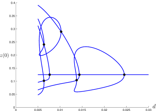
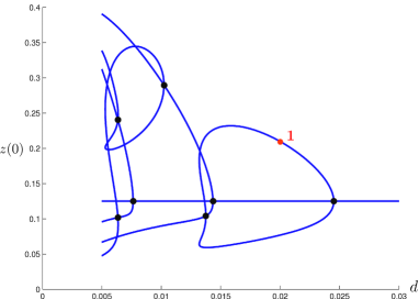
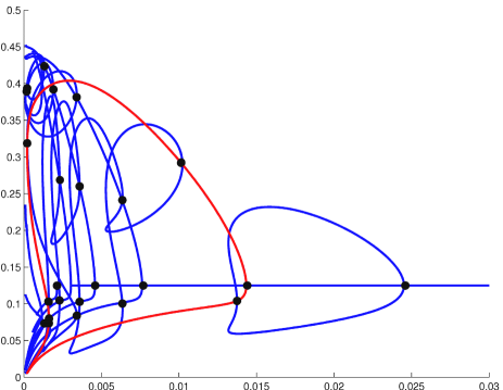
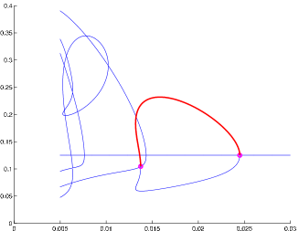
Let us present a consequence of Theorem 1. This result could be hard to prove with a purely analytic approach. Its proof is presented in Section 5 and see Figure 2 for a representation.
Corollary 1 (Co-existence of non constant steady states).
The following result may be a step toward rigorously studying steady states of the cross-diffusion model (2). Its proof is omitted since similar to the proof of Theorem 1.
Theorem 2 (Rigorous computations of approximations for a cross-diffusion model).
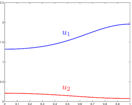

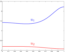
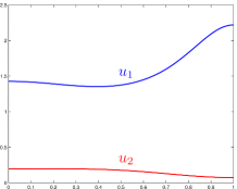
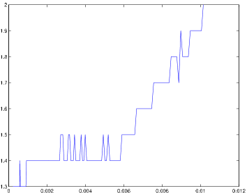
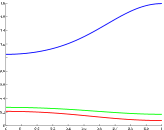
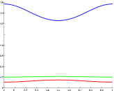
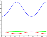
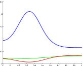
The solutions in Figure 3 are rigorously computed using the method presented in this paper. In fact the computation uses a simpler version of the method because the proofs of existence are only done at discrete values of the parameters. As can be seen in Table 1, there is apparent convergence as goes to zero. The bounds there are rigorous because we control through (the radius of the ball (7)) the error we have made with the numerical approximations. According to the work of [10], the solution on Figure 3(e) given by when should be close to a solution of the cross-diffusion system (2).
| 0.2918 | ||
| 0.0757 | ||
| 0.0092 |
The paper is organized as follows. In Section 2, the general method is introduced. In Section 3, the method is applied to the problem of computing rigorously steady states of the 3-component reaction-diffusion system (1), where the radii polynomials are explicitly constructed in this context. In Section 4, a detailed analysis of the optimal choice of the parameters , and is made, with the goal of maximizing the chances of performing successfully the computational proofs. Finally, in Section 5, the proofs of Theorem 1 and Corollary 1 are presented.
2 Description of the general method
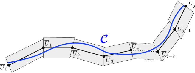
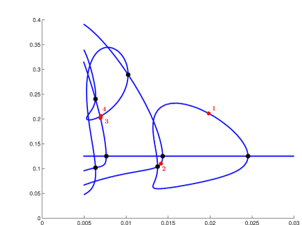
In this section, we present the general method, leaving some technical details to Section 3, where all the computations and estimates are presented explicitly to compute several global smooth branches of steady states of (1). The attention is now focused on describing a general method to prove existence and compute global smooth solution curves of in a Banach space of fast decaying Fourier coefficients. The method is based on the radii polynomials, first introduced in [12], and is strongly influenced by the rigorous branch following method of [11]. The idea is to compute a set of numerical approximations of by considering a finite dimensional projection, to use the approximations to construct a global continuous curve of piecewise linear interpolations between the ’s (see Figure 5) and to apply the uniform contraction principle on tubes centered at each segment to conclude about the existence of a unique smooth solution curve of nearby the piecewise linear curve of approximations. The approximate curve is computed using pseudo-arclength continuation (e.g. [13]).
2.1 Construction of a piecewise linear curve of approximations
To construct a piecewise linear curve of approximations of , we consider a finite dimensional projection of whose dimension depends on (see Section 3.1). In what follows, denotes considering this finite dimensional projection. Reversely, when we have some finite dimensional vector , denotes the infinite vector obtained by completing with zeros.
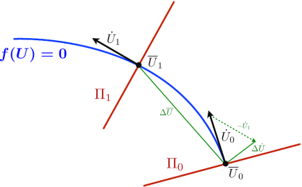
Suppose we have an approximate zero of at . Then, given , we compute an approximate tangent vector , that is Consider
| (8) |
a predictor, where is a parameter (whose value, representing roughly the arc length of curve we are covering in one step, is discussed in Section 4.1). Consider also the plane whose equation is given by . The pseudo-arclength operator is
and using Newton’s method with initial point , we compute such that . We refer to Figure 4 for a geometrical representation of a pseudo-arclength continuation step. A next predictor-corrector step can be performed starting at , and so on.
Applying the predictor-corrector step times, we compute a set of approximations that defines a piecewise linear approximation curve (see Figure 5). The next step is to show existence of a unique smooth solution curve of nearby the piecewise linear curve of approximations, as portrayed in Figure 5. This task is twofold. First, one shows the existence of a unique portion of solution curve in a small tube centered at the segment . This is done in Theorem 3 by showing that a Newton-like operator is a uniform contraction on the tube. To verify the hypothesis of the uniform contraction principle, Theorem 4 is introduced. This requires the construction of some bounds, which are presented in Section 2.2.1. In practice, verifying the hypothesis of Theorem 4 is done via Lemma 2 by using the radii polynomials which are presented in Section 2.2.2. From Lemma 2, one sees that the strength of the radii polynomials is that they provide an efficient means (in the form of a finite number of polynomial inequalities to be checked rigorously on a computer using interval arithmetic) of finding a set on which is a uniform contraction. Second, one shows that each is smooth, and that
is a global smooth solution curve of . In Section 2.3, we show how the smoothness of can be proved by verifying the hypothesis of Theorem 5. Afterward, we show that if the hypotheses of Theorem 5 and Theorem 6 are satisfied, then and connect smoothly. The smoothness of the global solution curve follows by construction.
2.2 Newton-like operator, uniform contraction and radii polynomials
Let us define what is required to prove existence of some portion of smooth curve . Without loss of generality, let us introduce the idea to prove the existence of that is the piece of curve close to the segment with two approximate tangent vectors and at those points given by the pseudo-arclength continuation algorithm. For any in , we set
and
Then we define, still for in , the hyperplane whose equation is given by
| (9) |
the function
| (10) |
and the Newton-like operator
| (11) |
where is an injective linear operator approximating the inverse of (see Section 3.2 for an example of how to construct and check that it is injective). We now use the uniform contraction principle on to conclude about the existence of a curve of fixed points that corresponds, by injectivity of , to a solution curve of .
Theorem 3.
If there exists some such that
is a uniform contraction, then for every , there exists a unique such that . Moreover, the function is of class if is of class .
Proof.
This is a direct application of the uniform contraction principle (e.g. see [14]). ∎
It seems legitimate to expect to be a contraction on a small set containing the segment parameterized by () since is an approximate Newton operator at .
2.2.1 Definition of some bounds
To prove that is a uniform contraction on , we prove the existence of bounds , , and such that for every and ,
| (12) |
| (13) |
The subscript corresponds to the first entry of and the first entry of . We set , where (same for ). Absolute values and inequalities applied to vectors are considered component-wise. For the sake of simplicity of the presentation, we omit to write explicitly the dependence of those terms in and when we are not focusing on them. Let us now give some sufficient conditions on those bounds for to be a uniform contraction.
Theorem 4.
Proof.
For all , , , the mean value theorem yields the existence of for some , such that
Then
Similarly,
Therefore, for all and ,
and for all and ,
∎
Suppose the bounds and verifying conditions (12) and (13) are computed. To be able to use Theorem 4, we need to check that those bounds also verify inequality (14). Note that for every , is a function of and is a function of both and . Besides, they can be constructed as polynomials in and , and for greater than some , we can choose
where is also a polynomial in and . Those assertions are not explained in details here. We refer to Section 3.6.2 and Section 3.7.3 for explicit details. For the moment, let us only say that can be taken to be for n large enough because has only a finite number of non zero coefficients, and hence for large enough. Let us now introduce the radii polynomials which allow us to verify inequality (14) using rigorous numerics.
2.2.2 Radii polynomials
Let be a computational parameter. We refer to Section 3.6 to determine how to choose its value. Define
for ,
and for ,
Note that the term has to be understood component-wise.
Lemma 2.
Proof.
By definition of the radii polynomials, we have that
for all . Since , we also have that
for all . Therefore inequality (14) is satisfied. ∎
2.3 Constructing a global smooth solution curve
Suppose now that we found satisfying the radii polynomials inequalities of Lemma 2. Hence, by Theorem 3, there exists a smooth function whose image is the only solution curve to within in a small tube of radius centered at the segment . More precisely, this tube is given by . The following result is similar to Lemma 10 in [11].
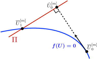
Theorem 5.
Suppose that
| (15) |
where
then is a smooth curve, that is, for all , .
Proof.
In practice, the hypothesis of Theorem 5 are checked rigorously using interval arithmetic. Remark that this hypothesis is very reasonable if is small enough. See Figure 6 for a geometric representation of the important quantities involved in the hypothesis (15). One can see there that if the length of the segment is small, that is if the vector is small, then the vectors and should be close to be perpendicular and the vectors and should be close to be parallel. Hence, should be close to the value while the vector should be close to . Hence, for very small value of , the value of should be small, and then the chances of satisfying inequality (15) should be high.
Assuming that two consecutive smooth curves have been computed, we can prove that they connect smoothly in one curve. Using the notation (resp. ) to refer to the first (resp. the second) portion of curve. The following result is similar to Proposition 8 in [11] but two aspects are different. First the gluing of and comes for free from the representation of the union of the segments and . Second, the proof that is smooth at the intersection is more detailed and calls upon the implicit function theorem.
Theorem 6.
Proof.
Since Theorem 4 is satisfied over the segment (resp. ), consider the radius (resp. ) satisfying (14). Without loss of generality, one can assume that by continuity of the radii polynomials. Theorem 4 allows us to use Theorem 3 to get the existence of two smooth functions and whose images are and . First we prove that the two curves connect, that is . Recalling (10), we have that , in particular and . Moreover, is the only solution of in and is the only solution of in . Hence and are both solutions to and since one of the two balls must be included into the other (they have same center) the two solutions are equal.
From now we assume without loss of generality that and we show that the connection between the two curves is smooth. For all in , the radii polynomials are negative at . The fact that the radii polynomials are continuous in yields the existence of such that those polynomials are still negative for in , and then that is still a uniform contraction for . As a result, can be extended into a smooth function defined on such that , for all in . Hence, . We want to find such that for all . To do that, set
We have and , so
Since the hypothesis of Theorem 5 is verified, we get according to (16) that . Hence the implicit function theorem holds and there exist and a smooth function , such that and . Also,
and since
we have that . Hence, there exists such that for all , and . Given that for all , has a unique solution in , showing that will conclude the proof. Now,
Using that , that is continuous and that , there exists , such that for all ,
By uniqueness, . ∎
The following result can be used to determine that a path of solution does not undergo any secondary bifurcations.
Corollary 2.
Proof.
According to (12), we have that
Since , we get that
Hence
because and have non negative entries and (14) holds. So we have that
We get that is invertible (its inverse is given by ), and so is injective. Let us show that for every , . Suppose by contradiction that . Let two linearly independent non-trivial vectors such that . Since is injective,
Hence, and , and then we can define . We conclude that . This is a contradiction. Hence . The derivative of the relation with respect to is given by
We showed in the proof of Theorem 5 since (15) holds, that . Hence, for every , , meaning by definition that is a regular path. ∎
3 Application to a 3-component reaction-diffusion PDEs
In this section, we present all quantities and estimates to construct explicitly the radii polynomials required to apply the theory of the general method of Section 2 to the problem of computing rigorously global smooth branches of steady states of the system of three reaction-diffusion PDEs given by (1). The first step is to consider a Galerkin projection of given in .
3.1 Finite dimensional projection
Given a finite dimensional parameter , denote to be and to be . The finite dimensional Galerkin projection of is
where for ,
| (17) | |||||
3.2 Explicit construction of the contraction
To define the Newton-like operator given in (11), remember that we have to build an injective linear operator which approximates the inverse of (with an approximate zero of given by a predictor-corrector step). Since
we take
| (18) |
where is a numerical inverse of that is
and () is a matrix defined as
| (19) | |||||
is the inverse of the linear part of . The idea behind this choice is explained soon and its interest will appear concretely in Section 3.7.2. To prove that is really injective, we compute using interval arithmetic and check that its value is less than one, and then prove that the matrices () are invertible (we only need to check using interval arithmetic that for all , and , since with the values of the parameters we are considering).
3.3 Verifying that and bootstrap argument
Remark that because of the terms, goes from the space to the space . Indeed, since is a Banach algebra (see Section 3.5), the non linear terms in do not affect the decay rate of . However, thanks to the choice of , defined by (18) goes from to so that . Remark that if , we cannot directly conclude that the solution of is a strong solution of (1). However, since , then (1) becomes
where each right-hand-side is in (here again we use the fact that is a Banach algebra). One can then easily see by dividing on both sides by that is in fact in . We can repeat this bootstrap argument to prove that any zero of lying in some () is in fact in every for and hence corresponds to steady states of (1). Furthermore, the estimates of Section 3.5 can be used to get explicit bounds for derivatives of any order for those solution functions, even if we did the proof with a .
We are almost ready to compute explicitly the bounds and and the radii polynomials. But to do so, we need to compute and to bound the convolution product that appear in it. That is what we do in the next two sections.
3.4 Computation of and
3.5 Analytic estimates
In order to bound all terms in (20) and (3.4), in particular quantities like , for , we have to develop some analytic estimates. Similar estimates have been produced for the case (e.g. [15]), but not for the case . From these estimates, we get that is a Banach algebra for each . First notice that, for all ,
Thus, what we need to show is that
is bounded for . We start by rewriting . If ,
and if ,
| (22) | |||||
In everything that follows, is a computational parameter (the larger is, the sharper the estimates will, but the greater the computational cost for the evaluation of the estimates will be) and is another computational parameter (which is taken equal to , see Section 3.6). First we define, for
| (23) |
and the unique zero of in . Note that is increasing on , goes to as goes to and to as goes to , so is well defined. Then we define
and finally
| (24) |
Proposition 1.
Let , and computational parameters. For all ,
This allows us to state the following result.
Lemma 3.
Let , , and computational parameters. For all ,
This bound, in addition of being very useful later in this paper, proves that is a Banach algebra for .
Proof.
(of Proposition 1) The bound for is due to [15]. We prove the bound for . The case is a direct consequence of the following inequality applied to (22)
For the case , let us consider the difference
Using (22) and the inequality below
we get that
| (25) | |||||
The first term of (25) can be bounded from above as follows
| (26) | |||||
The last inequality is due to the fact that for all , the series expansion
is an alternating series for (recall that ). According to (26), we have to bound and . First,
and then,
| (27) |
Similarly
and then
| (28) |
According to (26), (27) and (28), we get
| (29) |
Then we bound the second term of (25) from below
| (30) |
Using (25), (29) and (30) , we get
| (31) |
Now, if then and hence for all , . Thus
If then and we have two cases. The first case is that decreases until becoming negative for some which implies that for all . The second case is that stays positive for all which implies that is decreasing for all . In both cases we get that for all and thus
∎
Notice that since , (31) shows that . We could do the same kind of computation to bound from below and show that in fact . So the bound for is optimal, the only thing that can be improved is the way we approximate (which depends of ). But this also shows that the bound for may not be optimal, in fact it becomes quite bad when is close to since . However, if sharp estimates are needed for close to , there is a numerical way to get almost optimal bounds which is detailed it in Appendix A.1. We now give other bounds that are sharper for by using computations. Let us define
and
Lemma 4 (Sharper estimates).
Let , , and computational parameters, . for all
Proof.
We can split the summation in two parts :
The first one is exactly . We now bound the second one :
∎
Remark 1.
, the unique zero of in defined in (23), is increasing in and converges rather rapidly towards a bounded value. In particular, for (which is always the case for the proofs presented in this work), one has that . Numerically, the limit when goes to is about .
3.6 Computation of
According to (12), we focus here on
Remember that absolute values and inequalities applied to vectors or matrices should be understood component wise. Observe that so that
Because of the shape of in (18), we compute separately the bounds for and .
3.6.1 Case
Following the notation introduced earlier, is the vector containing and for any . We want to bound the quantity
With the expression and a Taylor expansion, we get that
which can be bounded, for , by
We see in Section 3.8 that we can get a uniform bound in by taking in the expression above. This uniform bound is simple to get but not the sharpest. We actually show in Appendix A.2 how to compute a sharper bound. The vectors and are computed with the expressions (20) and (3.4) by truncating the convolution products as in (3.1). This is a finite computation. We can set
3.6.2 Case
For ,
We can then set
The terms and are computed with the expressions (20) and (3.4). We can compute in a finite number of operations, because for any , and . In particular, for any , and we can take , so only a finite number of remains to be computed. Hence, setting , we have that for all , . In the next section, we see that for all , we can set . In fact, the value of is determined by the degree of the non linearities of . Here we have quadratic terms like
and with non linearities of degree , we would have the same by taking .
3.7 Computation of
For and , using a Taylor expansion, we get
| (32) | |||||
As for , we compute separately the bounds for and .
3.7.1 Case
For all , the shape of in (18) allows us to write
| (33) | |||||
where
and for all ,
Similarly,
and
can be bounded uniformly for by where
Notice that can be computed in a finite number of operations. According to (32) and (33), we have that for all ,
Using expression (3.4) and Lemma 4, we get that for all and ,
| (34) |
with and . Let us set
For , we know explicitly which allows us to compute sharper bounds. Still using (3.4), we get that for all , and ,
| (35) |
where
and
Let us also set
Observe that since has only a finite number of non-zero coefficients, can be computed in a finite number of operations.
Using all the bounds obtained in this section and the definition of in (13), we can define and the first by
where
3.7.2 Case
3.7.3 Case
We still have
but here we bound the convolution products in using Lemma 3 to get, for all ,
Then we set
and since the terms of and are decreasing for ( with the values of the parameter taken here, is always taken such that ), we can set, for all ,
| (36) |
Notice that (36) is what allows us to check the hypotheses of Theorem 3 with finite computations so it is really crucial for the proof, and we are able to do this thanks to the fact that the terms of are decreasing, which happens because the magnitude of the eigenvalues of the linear part of are growing in . In fact, we would have (36) for every system whose equations can be written as the sum of a linear operator with eigenvalues of increasing magnitude and a non linear polynomial term (in particular for reaction-diffusion systems).
3.8 Explicit computation of the radii polynomials
Now according to Section 2.2.2 and using the bounds and we got in the two previous sections, we define the radii polynomials. Notice that does not depend on and that has linear and quadratic terms in , so the radii polynomials are all of degree two.
3.8.1 Case
Let us set
| (37) | |||||
and
Then we define
and for all ,
3.8.2 Case
For , define
| (38) |
| (39) |
and
Then for each , we define
3.8.3 Case
3.8.4 Procedure to find (if possible) satisfying (14)
To verify hypothesis (14) of Theorem 3, we use Lemma 2. More explicitly we look for such that, for all , and for all . Notice that the coefficients of the radii polynomials are increasing with so that it is equivalent to find such that
| (41) |
To find such , we set
| (42) |
Then we determine numerically an approximation of
| (43) |
If , we choose , and check (41) rigorously, by computing the coefficients of the radii polynomials with using interval arithmetic. We see in Section 4.1 why it is reasonable to hope that such exists, provided the parameters , and are chosen carefully.
4 Optimization of the parameters
4.1 Optimal choice of the parameters and
Recall that the parameter controls the dimension (which equals ) of the finite dimensional Galerkin projection given by (3.1), and from (8), the parameter is used to define a predictor whose value serves as an initial point for Newton’s method to get a corrector . The value of represents roughly the arc length of curve we are covering in one predictor-corrector step, hence the name pseudo-arclength continuation. Since , if is not so large, then its value should be close to the length of the segment . Hence, studying is roughly the same as studying the length of .
The optimal strategy aims at maximizing the pseudo-arclength parameter to prove existence of long pieces of solution curve in one predictor-corrector step (as explained in Section 2.1) while taking as small as possible in order to minimize the computational cost. However, the fact that we are looking for an verifying the hypotheses of Theorem 3 (which is equivalent to find for which every radii polynomial is negative) leads to some constraints.
Let us now remark that for a quadratic polynomial of the form , if , and is small enough (precisely ), then there is an interval such that for all , . Based on this fact, let us study in details the coefficients of each radii polynomial to see how to choose and optimally. Since we showed in Section 3.8 that we could bound the polynomials letting , we always set from now .
4.1.1 Case
Recall the definition of the coefficients , and of the radii polynomials for the case . First notice that each component of and is positive. In the definition of , the first two terms are very small (the first by definition of , and the second provided is not too small, which will always be the case), and the next two can be made as small as needed (and so will be negative) by taking small enough. can also be made very small by taking small (see Section 3.6.1). Hence we can expect each set (for ) defined in Section 3.8 to be non empty if is small enough (the same is true for ).
4.1.2 Case
Recall the definition in Section 3.8.2 of the coefficients , and of the radii polynomial for the case . According to the previous section, should not be too large and hence here again should be small. Also, the predominant term of in (39) is which decreases to as grows, so taking large enough should allow us to have negative for and thus, recalling (42), we can expect that (for ).
4.1.3 Case
The situation in the case is the same as above except that the expression of in (40) is different, with large enough we can expect to be non empty.
4.1.4 Algorithm to choose and optimally
Let us now present an algorithm to chose and optimally. Given , , and ,
The fact that we try to increase and decrease after each successful step is not optimal. We indeed observed numerically that the process often failed. In fact we noticed that the value of has to reach some threshold before could be increased successfully. Similarly has to reach some other threshold before could be decreased successfully. In practice we only try to increase or decrease if those thresholds are reached.
Note that we want to change the value of along the process while conserving the smoothness property of the global curve. The important fact is to have exactly the same function given by (10) at the end of one piece of curve and at the start of the next, that is with the notations of Section 2.3, and this even when we change the value of between the two. Let us denote (resp. ) the value of for the first curve (resp. the second). In , only changes with . Hence, we only need to check that . Remember that and are constructed from finite dimensional vectors and completed with zeros. In fact, and . If we increase , that is , the last frequencies of (that is , for ) are zeros and hence is equal to . Decreasing , that is , requires a bit of care since the last frequencies of are not necessarily zero. Hence we have to make an intermediate step. Let us denote the last point we have and a tangent vector at this point. From there, we make a new predictor-corrector step with equal to , get a point and then compute . Before doing the proof of this portion of curve, we set the frequencies of and to zero. Then we are able to decrease at the next step while having exactly the same at the connecting point.
4.2 Optimal choice of the decay rate parameter
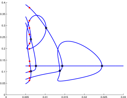
In light of Lemma 1, computing steady state of (1) with Neumann boundary conditions is equivalent to find such that , and that for any fixed . Hence, it seems legitimate to investigate which decay rate is optimal. The weight defined in (4) depends on and it influences the value of the norm and the theoretical bounds of Lemma 3. Since the value of has a major impact on the radii polynomials, it influences strongly the values of the parameters and used for the proof, and therefore it influences the computational time required to perform the proofs. As one can see in Table 2, depending on the value of , the computational costs required to prove the red branches of Figure 10(a) and Figure 10(b) can change drastically. In Figure 7, one can see how influences the values of and while performing the algorithm of Section 4.1.4 along the first bifurcation branch presented in red in Figure 10(a), and along the first part of the second bifurcation branch presented in red in Figure 10(b).
| Red branch of Figure 10(a) | Red branch of Figure 10(b) | |
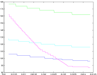
What we see with these comparisons is that, on the red branch of Figure 10(a), taking smaller allows using a greater but at the expense of a greater . Hence, a better compromise seems to be somewhere between and . But it seems that when becomes small, it could also be better to take smaller in order to use a smaller (see the case on Figure 7(d)). Let us see how this evolves when becomes even smaller. Note that we were able to get the rigorous data (for different values of ) of Table 2 and of Figure 7 because the rigorous computations of the concerned branches did not take too long. However for some other curves, the proof takes much longer, mainly because gets smaller and hence must be taken larger for the coefficients of the last radii polynomial (40) to be negative. On the other hand, it only takes one point along the branch to determine, given , which value of should be taken in order to make negative. Also, the cost of the proof decreases linearly with but increases quadratically with , so it seems fair to chose according to only and independently of for those branches where has to be taken large. In Figure 8(a), we present some non rigorous results concerning the second part of the second branch. Although non rigorous, these results helps understanding the role played by for the computational cost of the method. We can see in Figure 8(b) that as the diffusion parameter decreases, the optimal decay rate becomes smaller as well. That can be explained by the fact that the coefficient of the last radii polynomial is non negative if is taken too small. A necessary condition for to be negative is roughly the following
which shows why has to be taken larger when becomes smaller. But to understand the impact of , we have to detail how the values of and evolve with . For this let us recall the definitions of in (5) and of in (24) and let us look at the shape of the solution . For instance, we see on Figure 9(b) that on the first branch the solutions are almost sinusoids of period and hence . Hence, taking smaller does not decrease the value of , but it increases slightly , and then finally leads to a greater . However, when becomes smaller, the high frequencies in the solutions are more and more important. Thus involves for some and hence taking smaller decreases significantly the value of and therefore the value of . This allows taking a smaller , provided that is not too small. Indeed, increases more than decreases when gets close to , which explains why the optimal value of seems not to go below . One can see in Figure 8(b) that when is really small, the value of is far much smaller with than with . This is a significant improvement, especially in terms of the computational cost which evolves in . Actually, we did some computation, and the cost of the proof to do part of a branch for small is about times faster with than with . This brings us to the conclusion that the new estimates introduced in Section 3.5 for can be quite useful. Actually, they allowed proving parts of some branches in Figure 8(a) which we would not have been able to do with .
![[Uncaptioned image]](/html/1511.01414/assets/x16.png)
![[Uncaptioned image]](/html/1511.01414/assets/x24.png)
![[Uncaptioned image]](/html/1511.01414/assets/x26.png)
5 Proofs of two main results of Section 1
5.1 Proof of Theorem 1
Recall (7) and fix . Set in the bounds of Lemma 3 and set in those of Lemma 4. Set the multiplicative coefficient used to change equal to and the one used to change equal to . That means that in the algorithm of Section 4.1.4, taking larger means setting , taking smaller means setting , taking larger means setting and taking smaller means setting . We proved that in a small tube (whose size is given by ) of each portion of curve represented in Figure 1 between two bifurcation points, there exists a unique smooth curve representing exactly one steady states of (1). Note that the method cannot prove that those curves really reach the bifurcation points, but we can virtually go as close as we want to those bifurcation points, the only limit being the computational cost. On the other hand, applying the result of Corollary 2, we can conclude that along the rigorously computed smooth branches, there are no secondary bifurcation of steady states. In Table 2, Figure 7 and Figure 9, one has some example of the parameters used, the running time required to compute the branches and some spatial representations of solutions on different branches. ∎
5.2 Proof of Corollary 1
Consider one portion of branch we have proven. We have the existence of a smooth function (defined on ) parametrising our portion of curve, and we know that it lies in a tube of radius around our numerical solution. So we know the initial point and the final point with a precision of in . In particular, if (respectively ) is the numerical value of from which the branch starts (respectively at which the branch finishes) then there exists a in and a in such that and . Thus, if the branch we are considering is such that
or reversely
then the intermediate value theorem yields the existence of an in such that . Notice that if is too close to or for those hypothesis to be satisfied, you just have to consider several consecutive portions of curve rather than a single one. On the diagram we proved, there are eleven such portions (see Figure 2). To complete our proof, we need to check that each solution is different from one another, and we are able to do this because the radius we get in our proofs are small enough. Remember that what we are representing on our bifurcation diagram is the value of at and that
Besides we know that so
In fact, the quantity is the one we represented on the diagram, and so the error we did by using this representation is bounded by
With the value of we used and the we got, those were always smaller than and hence the error we made are in fact lying in thickness of the line on the diagram, so we are sure that we have eleven different solutions. ∎
Appendix A Appendix
A.1 Sharper estimates for
What we have already proven in the proof of Proposition 1 in (31) is that, for all and
and since we needed a uniform bound, we took . Since , we would like to take and hence larger to improve the estimate, but the point of getting a sharp estimate is to allow us to take smaller, so this does not really make sense. However, there is a way to rigorously compute a bound that is almost optimal, without increasing . Let , , , and since is deceasing such can be computed numerically and rigorously using interval arithmetic. Then we have that, for all
the max being computed rigorously using interval arithmetic. We can have a bound as sharp as we want by taking small, but at the expense of some computational cost which is in . Indeed, when goes to , is equivalent to and hence .
A.2 Sharper uniform bounds for for
To prove that is a uniform contraction, we have in Section 3.6 to bound uniformly in terms of the form for in . We did that the simplest way, using triangular inequality to say that
However, given the expression of , we can get a better bound which depends on whether the apex of is between and or not. More explicitly,
References
- [1] Yukio Kan-on and Masayasu Mimura. Singular perturbation approach to a -component reaction-diffusion system arising in population dynamics. SIAM J. Math. Anal., 29(6):1519–1536 (electronic), 1998.
- [2] Rui Peng and Mingxin Wang. Pattern formation in the Brusselator system. J. Math. Anal. Appl., 309(1):151–166, 2005.
- [3] Michael G. Crandall and Paul H. Rabinowitz. Bifurcation from simple eigenvalues. J. Functional Analysis, 8:321–340, 1971.
- [4] Paul H. Rabinowitz. Some global results for nonlinear eigenvalue problems. J. Functional Analysis, 7:487–513, 1971.
- [5] Masato Iida, Masayasu Mimura, and Hirokazu Ninomiya. Diffusion, cross-diffusion and competitive interaction. J. Math. Biol., 53(4):617–641, 2006.
- [6] A.M. Turing. The chemical basis of morphogenesis. Phil. Trans. R. Soc. Lond. B, 237:37–72, 1952.
- [7] Herbert Amann. Nonhomogeneous linear and quasilinear elliptic and parabolic boundary value problems. In Function spaces, differential operators and nonlinear analysis (Friedrichroda, 1992), volume 133 of Teubner-Texte Math., pages 9–126. Teubner, Stuttgart, 1993.
- [8] Y. S. Choi, Roger Lui, and Yoshio Yamada. Existence of global solutions for the Shigesada-Kawasaki-Teramoto model with weak cross-diffusion. Discrete Contin. Dyn. Syst., 9(5):1193–1200, 2003.
- [9] Yuan Lou, Wei-Ming Ni, and Yaping Wu. On the global existence of a cross-diffusion system. Discrete Contin. Dynam. Systems, 4(2):193–203, 1998.
- [10] Hirofumi Izuhara and Masayasu Mimura. Reaction-diffusion system approximation to the cross-diffusion competition system. Hiroshima Math. J., 38(2):315–347, 2008.
- [11] Jan Bouwe van den Berg, Jean-Philippe Lessard, and Konstantin Mischaikow. Global smooth solution curves using rigorous branch following. Math. Comp., 79(271):1565–1584, 2010.
- [12] Sarah Day, Jean-Philippe Lessard, and Konstantin Mischaikow. Validated continuation for equilibria of PDEs. SIAM J. Numer. Anal., 45(4):1398–1424 (electronic), 2007.
- [13] H. B. Keller. Lectures on numerical methods in bifurcation problems, volume 79 of Tata Institute of Fundamental Research Lectures on Mathematics and Physics. Published for the Tata Institute of Fundamental Research, Bombay, 1987. With notes by A. K. Nandakumaran and Mythily Ramaswamy.
- [14] Shui Nee Chow and Jack K. Hale. Methods of bifurcation theory, volume 251 of Grundlehren der Mathematischen Wissenschaften [Fundamental Principles of Mathematical Science]. Springer-Verlag, New York, 1982.
- [15] Marcio Gameiro and Jean-Philippe Lessard. Analytic estimates and rigorous continuation for equilibria of higher-dimensional PDEs. J. Differential Equations, 249(9):2237–2268, 2010.