Abstract

Let $M$ be a compact manifold equipped with a pair of complementary foliations, say horizontal and vertical. In Catuogno, Silva and Ruffino [5] it is shown that, up to a stopping time $\tau$, a stochastic flow of local diffeomorphisms $\varphi_{t}$ in $M$ can be written as a Markovian process in the subgroup of diffeomorphisms which preserve the horizontal foliation composed with a process in the subgroup of diffeomorphisms which preserve the vertical foliation. Here, we discuss topological aspects of this decomposition. The main result guarantees the global decomposition of a flow if it preserves the orientation of a transversely orientable foliation. In the last section, we present an Itô-Liouville formula for subdeterminants of linearised flows. We use this formula to obtain sufficient conditions for the existence of the decomposition for all $t\geq 0$.

Key words: Stochastic flow of diffeomorphisms, decomposition of diffeomorphisms, biregular foliations, tranversely orientable foliation.

MSC2010 subject classification: 60H10, 58J65, 57R30.

1 Introduction

Consider a stochastic flow $\varphi_{t}$ of diffeomorphisms in a compact differentiable manifold $M$ endowed with some structure (Riemannian, Hamiltonian, foliation, etc). In many situations, the decomposition of $\varphi_{t}$ with components in subgroups of the group of diffeomorphisms $\mathrm{Diff}(M)$ provide interesting dynamical or geometrical information of the stochastic system. In the literature, this kind of decomposition has been studied in several frameworks and with different aimed subgroups; among others, see e.g. Bismut [1], Kunita [9], [10], Ming Liao [13] and some of our previous works [4], [6], [15], [19].

In particular, in Catuogno, da Silva and Ruffino [5], the authors consider a pair of complementary distributions in a differentiable manifold $M$, in the sense that each tangent space splits into a direct sum of two subspaces depending differentiably on $M$. These subspaces are called, by convenience, horizontal and vertical distributions. In [5] it is shown that locally, up to a stopping time $\tau$, a stochastic flow $\varphi_{t}$ in $M$ can be decomposed as $\varphi_{t}=\xi_{t}\circ\psi_{t}$, where $\xi_{t}$ is a diffusion in the group of diffeomorphisms $\mathrm{Diff}(\Delta^{H},M)$ generated by horizontal vector fields, and $\Psi_{t}$ is a process in the group of diffeomorphisms $\mathrm{Diff}(\Delta^{V},M)$ generated by vertical vector fields. The authors also present stochastic differential equations on the corresponding infinite dimensional Lie subgroups for the components $\xi_{t}$ and $\psi_{t}$. The infinite dimensional Lie group structure considered in this case is described in Milnor [16], Neeb [17] and Omori [18]. The stopping time $\tau$ mentioned above, which restricts the time where the decomposition exists, appears due to an explosion in the equation of one of the components of the decomposition, with initial conditions at the identity. It is related to the degeneracy of the dynamics of one distribution with respect to the other.

The initial motivation for this kind of decomposition comes from a system whose flow is originally energy perserving, hence trajectories lies on energy levels. After a perturbation by transverse vector fields, hence destroying this foliated behaviour, the decomposition allows to study separatly an energy preserving component and a transverse component. This is, for instance the context of an averaging principle in Gargate-Ruffino [8], where the vertical component is rescaled by $\epsilon^{-1}$, see also Li [11] in the Hamiltonian context. Flows in a principal fibre bundle with an affine connection gives another class of examples where the distributions are not necessarily integrable, hence generating holonomy. In Melo, Morgado and Ruffino [14], the same decomposition is considered for the case of stochastic flows with jumps, using Marcus equation, as in Kurtz, Pardoux and Protter [12].

In this article, we work with the same structure of [5], but assuming that the distributions are integrable: The manifold $M$ is endowed with two complementary foliations $\mathcal{H}$ and $\mathcal{V}$, i.e., such that the leaves of the vertical foliation $\mathcal{V}$ are transverse to the leaves of the horizontal foliation $\mathcal{H}$, in the sense that $TM=T\mathcal{H}\oplus T\mathcal{V}$. We use the notation $(M,\mathcal{H},\mathcal{V})$ for this space. The action of the subgroup of diffeomorphisms $\mathrm{Diff}(\Delta^{H},M)$ fixes each horizontal leaf and the action of $\mathrm{Diff}(\Delta^{V},M)$ fixes vertical leaves. The dynamics in $M$ is given by a stochastic flow of (local) diffeomorphisms $\varphi_{t}$ generated by a Stratonovich SDE on $M$:

$$dx_{t}\ =\sum_{r=0}^{m}X_{r}(x_{t})\circ dW_{t}^{r},$$ (1)

where $W^{0}_{t}=t$, $(W^{1},\ldots,W^{m})$ is a Brownian motion in $\mathbf{R}^{m}$ constructed on a filtered complete probability space $(\Omega,\mathcal{F},\mathcal{F}_{t},\mathbf{P})$ and $X_{0},X_{1},\ldots,X_{m}$ are smooth vector fields in $M$. In this situation, there exists a stochastic solution flow of (local) diffeomorphisms $\varphi_{t}$, see e.g. among others the classical Kunita [9], Elworthy [7]. The flow is assumed to be complete, such that its explosion time is not a restriction for the decomposition. The fact that we deal with an stochastic flow of a Stratonovich SDE is convenient, say, to get explicit equations for the components $\xi_{t}$ and $\psi_{t}$, and to find an Itô formula for subdeterminants involved in the context (Section 3.1). Nevertheless, here, many of our results on decomposition apply also to a continuous family $\phi_{t}$ of diffeomorphisms such that $\phi_{0}=Id$, which not necessarily satisfies the cocycle property (e.g. Theorem 2.5).

Our aim here is to study topological features on the foliations relating to this decomposition. It is particularly interesting the fact that decomposability of a flow is strongly related with the geometrical concept of transverse orientation in a pair of foliations. Precisely, the influence of the topology of the foliations appears in two intertwined categories: analytical and topological aspects. The analytical approach is presented in Section 1.2. It is essentially guided by the subdeterminant of the linearised flow: it gives us a necessary and sufficient condition for the local existence of the decomposition.

For the topological aspects, initially, we consider a pair of horizontal and vertical foliations, where there might be a set of points which one can not reach from a point $x_{0}$ in the manifold $M$, by taking a concatenation of a vertical path with a horizontal path, in this order. We discuss this property of attainability and its consequences for the decomposition in Section 2.1. In Section 2.2, we study the dynamics of the stochastic flow $\varphi_{t}$ in the leaves, and how this action might be a restriction for the decomposition. Our main result is in Section 2.3, where we proof that, under the condition of transverse orientability of the horizontal foliation, the global decomposition exists if and only if the family of diffeomorphisms preserves this orientation.

In the last section we present an Itô-Liouville formula for subdeterminants of the linearized stochastic flow $D\varphi_{t}$. Using this formula and Cauchy-Binet identity (see e.g. Tracy and Widom [21]), we discuss a pair of sufficient condition for the existence of the decomposition of the flow $\varphi_{t}$, for $t\geq 0$.

1.1 Foliations

We recall briefly some geometrical facts about foliations in a differentiable manifold. For more details, see e.g., among many others, Candel and Conlon [3], Tamura [20], Walcak [22]. Let $M$ be a Riemannian manifold of dimension $n$.

Definition 1.1.

A foliation with codimension $k$ in $M$ is a partition $\mathcal{F}=\{\mathcal{F}(p):p\in M\}$ of $M$ endowed with a $C^{\infty}$-atlas $\{(\phi_{\alpha},U_{\alpha})\}_{\alpha\in\mathcal{I}}$ where

$$\begin{array}[]{crcl}\phi_{\alpha}:&U_{\alpha}&\rightarrow&\mathbb{R}^{n-k}\times\mathbb{R}^{k}\\ &p&\mapsto&(x_{\alpha}(p),y_{\alpha}(p)),\end{array}$$

such that each local chart $\phi_{\alpha}$ satisfies the property that if $y_{\alpha}(p)=y_{\alpha}(q)$, then $\mathcal{F}(p)=\mathcal{F}(q),$ for $p$ and $q$ in $U_{\alpha}$.

The atlas $\{\phi_{\alpha},U_{\alpha}\}$ above is called a foliated atlas. Each $\mathcal{F}(p)$ is called the leaf of $p$. A set $P\subset M$ is a plaque of the foliation $\mathcal{F}$ if it is an open submanifold of an $(n-k)$-dimensional leaf, precisely: $P$ has the form $P=\phi_{\alpha}^{-1}(D)$ where $D$ is an open disk of dimension $n-k$ contained in a level subset $\{p\in U_{\alpha}:y_{\alpha}(p)=y_{0}\}$. Each leaf of the foliation is the image of an immersion of a complete manifold into $M$. Given $N\subset M$ the saturation $\mathcal{F}(N)$ of $N$ by $\mathcal{F}$ is the set $\mathcal{F}(N)=\cup_{p\in N}\mathcal{F}(p)$.

With refinements, if necessary, one can always obtain a regular atlas $\{\phi_{\alpha},U_{\alpha}\}$, i.e. such that $U_{\alpha}$ is precompact in a bigger foliated domain, the cover $\{U_{\alpha}\}$ is locally finite and the interior of each closed plaque of $U_{\alpha}$ meets at most one plaque in the closure of $U_{\beta}$, see [3, Chap.1].

Given two local charts $(\phi_{1},U_{1})$ and $(\phi_{2},U_{2})$ in the regular foliated atlas $\{(\phi_{\alpha},U_{\alpha})\}$ such that $U_{1}\cap U_{2}\not=\emptyset$ we define the functions $y_{i}:\phi_{2}(U_{1}\cap U_{2})\rightarrow\mathbb{R}$ by $\phi_{1}\circ\phi_{2}^{-1}=(y_{1},...,y_{n}).$ Let $x_{i}$ denote the usual coordinates on $\mathbb{R}^{n}$, we say that the atlas $\{(\phi_{\alpha},U_{\alpha})\}$ is transversely orientable if

$$\det\displaystyle\frac{\partial(y_{n-k+1},...,y_{n})}{\partial(x_{n-k+1},...,x_{n})}>0$$

everywhere in the domain, for any two local charts $(\phi_{1},U_{1})$ and $(\phi_{2},U_{2})$ in $\{(\phi_{\alpha},U_{\alpha})\}$ with $U_{1}\cap U_{2}\not=\emptyset$. See an example of non-transversely orientable foliation in Example 2.7 below.

An important property we use in the next section is the uniform transverselity of the foliation, see e.g. Camacho and Lins-Neto [2]:

Theorem 1.2.

Consider a foliated space $(M,\mathcal{F})$ and a fixed leaf $F$. Given two $k$-dimensional submanifolds $N_{1}$ and $N_{2}$ which are transverse to $F$, there exist disks $D_{1}\subset N_{1}$ and $D_{2}\subset N_{2}$ and a diffeomorphism $f:D_{1}\rightarrow D_{2}$ such that for any leaf $F^{\prime}$ with $F^{\prime}\cap D_{1}\not=\emptyset$ we have that $f(F^{\prime}\cap D_{1})=F^{\prime}\cap D_{2}$.

For a pair of complementary foliations in $M$ we have:

Definition 1.3.

A birregular atlas on $(M,\mathcal{H},\mathcal{V})$ is an atlas $\{(\phi_{\alpha},y_{\alpha},U_{\alpha})\}_{\alpha\in\mathcal{I}}$ which is simultaneously a regular foliated atlas for $\mathcal{H}$ and $\mathcal{V}$.

It is well known that there always exists a birregular foliated atlas for $(M,\mathcal{H},\mathcal{V})$, see e.g. [3, Prop. 5.1.4].

1.2 Characterization of local decomposition

Consider a diffeomorphism $\varphi:U\rightarrow V$, with $U$ and $V$ open subsets of $\mathbf{R}^{n}$. The product $\mathbf{R}^{n-k}\times\mathbf{R}^{k}$ is a canonical Cartesian pair of foliations of $\mathbf{R}^{n}$. With respect to this product, write $\varphi=(\varphi^{1}(x,y),\varphi^{2}(x,y))$, i.e. $x$ and $\varphi^{1}(x,y)$ belong to $\mathbf{R}^{n-k}$ and $y,\varphi^{2}(x,y)\in\mathbf{R}^{k}$. An analytical restriction for the local decomposition of $\varphi$ appears related with the subdeterminant of the derivative of $\varphi$:

Proposition 1.4.

There exists a unique (up to reduction in the domain) decomposition $\varphi=\xi\circ\psi$ in a neighbourhood of $(x,y)$ if and only if

$$\det\frac{\partial\varphi^{2}(x,y)}{\partial y}\neq 0.$$

Moreover, if $t\mapsto\varphi_{t}$ is continuous (with respect to, say, $C^{k}$ topology) and satisfies the determinant condition above, then $\xi_{t}$ and $\psi_{t}$ are also continuous with respect to time $t$.

Proof.

In fact, if $\varphi_{t}=(\varphi_{t}^{1},\varphi_{t}^{2})$ then

$$\psi_{t}=(Id_{\mathbf{R}^{n-k}},\varphi_{t}^{2}),$$

and

$$\xi_{t}=(*,Id_{\mathbf{R}^{k}})=\varphi_{t}\circ\psi_{t}^{-1}.$$

The proof is a simple application of the theorem of inverse functions, see also Melo, Morgado and Ruffino [14]. Continuity of $\xi_{t}$ and $\psi_{t}$ follows directly from the continuity of the components in the formulae above.

∎

Applying this characterization into flows in $\mathbf{R}^{n}$, we have that there exists the decomposition of an stochastic flow $\varphi_{t}=\xi_{t}\circ\psi_{t}$ up to a stopping time $\tau$ in a neighbourhood of the initial condition $(x,y)$, where

$$\tau=\sup\{t>0;\det\frac{\partial\varphi_{s}^{2}(x,y)}{\partial y}\neq 0,\mbox{ for all }0\leq s\leq t\}.$$

In particular, if $(M,\mathcal{H,V})$ is a product space $M=H\times V$ with $H$ and $V$ two differentiable manifolds and a diffeomorfism $\varphi$ sends each vertical leaf entirely into a vertical leaf, then the determinant never vanishes, hence the decomposition $\varphi=\xi\circ\psi$ holds. For example, linear systems with spherical (horizontal) and radial (vertical) foliations in $\mathbf{R}^{n}\setminus\{0\}$: in this case, vertical leaves are sent to vertical leaves, hence the decomposition holds for all $t\geq 0$, see [14]. On the other hand, consider the simple example of a linear rotation in $\mathbf{R}^{2}$ endowed with the canonical Cartesian (horizontal and vertical) foliations. We have the decomposition:

$$\varphi_{t}=\left(\begin{array}[]{cc}\cos t&-\sin t\\ \sin t&\cos t\end{array}\right)=\left(\begin{array}[]{cc}\sec t&-\tan t\\ 0&1\end{array}\right)\left(\begin{array}[]{cc}1&0\\ \sin t&\cos t\end{array}\right).$$

Clearly, the vertical leaves are not preserved. There exists an analytical obstruction when $t=\frac{\pi}{2}$. So, the stopping time $\tau=\frac{\pi}{2}$. In the next section, the same example is interpreted as a topological obstruction at $t=\pi/2$, since the dynamics of vertical leaves collapses on horizontal leaves (Proposition 2.4).

2 Topological aspects on global decomposition

We distinguish three kinds of topological aspects of the foliations related with the existence of the decomposition: the first one concerns the limitation on the attainability of trajectories starting at an initial condition and running exclusively along a vertical trajectory concatenated with a horizontal trajectory. The second aspect concerns the effect of the dynamics on the leaves. Finally, the third aspect concerns transversely orientation of the horizontal foliation. Our main result guarantees that if the flow preserves this orientation, then the flow is globally decomposable.

2.1 Attainability

In many pairs of foliations, given a starting point $x_{0}$ there might be a set of points which one can not reach from $x_{0}$ by taking a concatenation of a vertical path with a horizontal path, in this order. See e.g. Figure 1, where, say the horizontal leaves are represented by bold curves and vertical leaves are represented by thin curves in $\mathbf{R}^{2}\setminus\{0\}$. For $x_{0}=(1,1)$, the attainable points is the open set above the line $y=-x$.

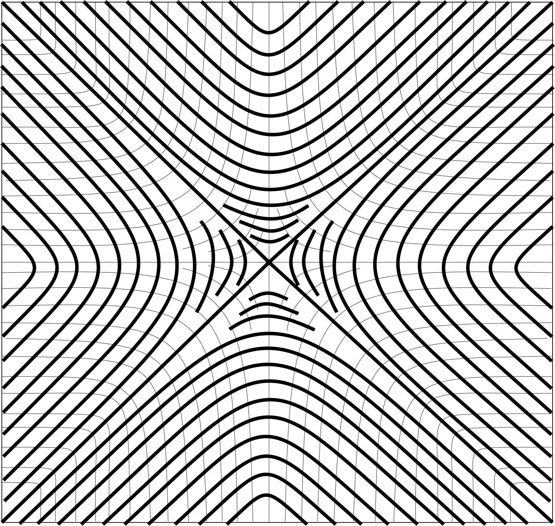
Figure 1: Pair of foliations with $\mathcal{A}(x)\neq M$.

This idea leads to the following:

Definition 2.1.

The attainable points from $x\in M$ with respect to the pair of foliations $(M,\mathcal{H},\mathcal{V})$ is the set

$$\mathcal{A}(x)=\mathcal{H}(\mathcal{V}(x)).$$

Clearly, $\mathcal{A}(x)$ is horizontally saturated and, if a diffeomorphism $\varphi$ is decomposable in a neighbourhood of $x$, then $\varphi(x)\in\mathcal{A}(x)$. Hence, non-attainability is an intrinsic obstruction for the decomposition. Thinking on reversibility and commutativity of the decomposition, we present the following:

Definition 2.2.

The co-attainable set of $x\in M$ with respect to the pair of foliations $(M,\mathcal{H},\mathcal{V})$ is the set

$$\mathcal{C}(x)=\mathcal{H}(\mathcal{V}(x))\cap\mathcal{V}(\mathcal{H}(x)).$$

A point $y\in M$ belongs to $\mathcal{C}(x)$ if $y\in\mathcal{A}(x)$ and $x\in\mathcal{A}(y)$. Note that, for each $x\in M$, the sets $\mathcal{A}(x)$ and $\mathcal{C}(x)$ are open since the leaves of $\mathcal{H}$ are everywhere transverse to the leaves of $\mathcal{V}$. Next we present a property of the attainable sets $\mathcal{A}(x)$.

Proposition 2.3.

Let $M$ be a compact connected manifold. If for a certain $x\in M$ we have $\mathcal{A}(x)=\mathcal{C}(x)$, then $\mathcal{A}(x)=M$.

Proof.

Consider $y\in\partial\mathcal{A}(x)$. Then $\mathcal{V}(y)\cap\mathcal{A}(x)\not=\emptyset,$ since $\partial\mathcal{A}(x)$ is an $\mathcal{H}$-saturated set. Therefore, there exists a $z\in\mathcal{V}(y)\cap\mathcal{A}(x)$. On the other hand, as $z\in\mathcal{C}(x)$, we have that $\mathcal{V}(y)\cap\mathcal{H}(x)\not=\emptyset$. Now let $\gamma$ be a horizontal curve starting at $x$ and ending at the point $w\in\mathcal{V}(y)\cap\mathcal{H}(x)$.

Using the fact that $\partial\mathcal{A}(x)$ is $\mathcal{H}$-saturated and that $M$ is compact we have that either all vertical leaves of $\mathcal{V}(\gamma)$ intersect $\partial\mathcal{A}(x)$ or none of them intersects $\partial\mathcal{A}(x)$. But we already know that $\mathcal{V}(w)=\mathcal{V}(y)$ intersects $\partial\mathcal{A}(x)$, therefore so does $\mathcal{V}(x)$. This implies that $\partial\mathcal{A}(x)\subset\mathcal{A}(x)$ and then $\mathcal{A}(x)=M$, since $M$ is connected.

∎

The converse of the proposition above obviously does not hold. Also, if $\mathcal{A}(x)=M$ it does not imply that $\mathcal{A}(z)=M$ for all $z\in M$. As a simple example, in Figure 2, $\mathcal{A}(x)=M$ but $y\notin\mathcal{A}(z)$.

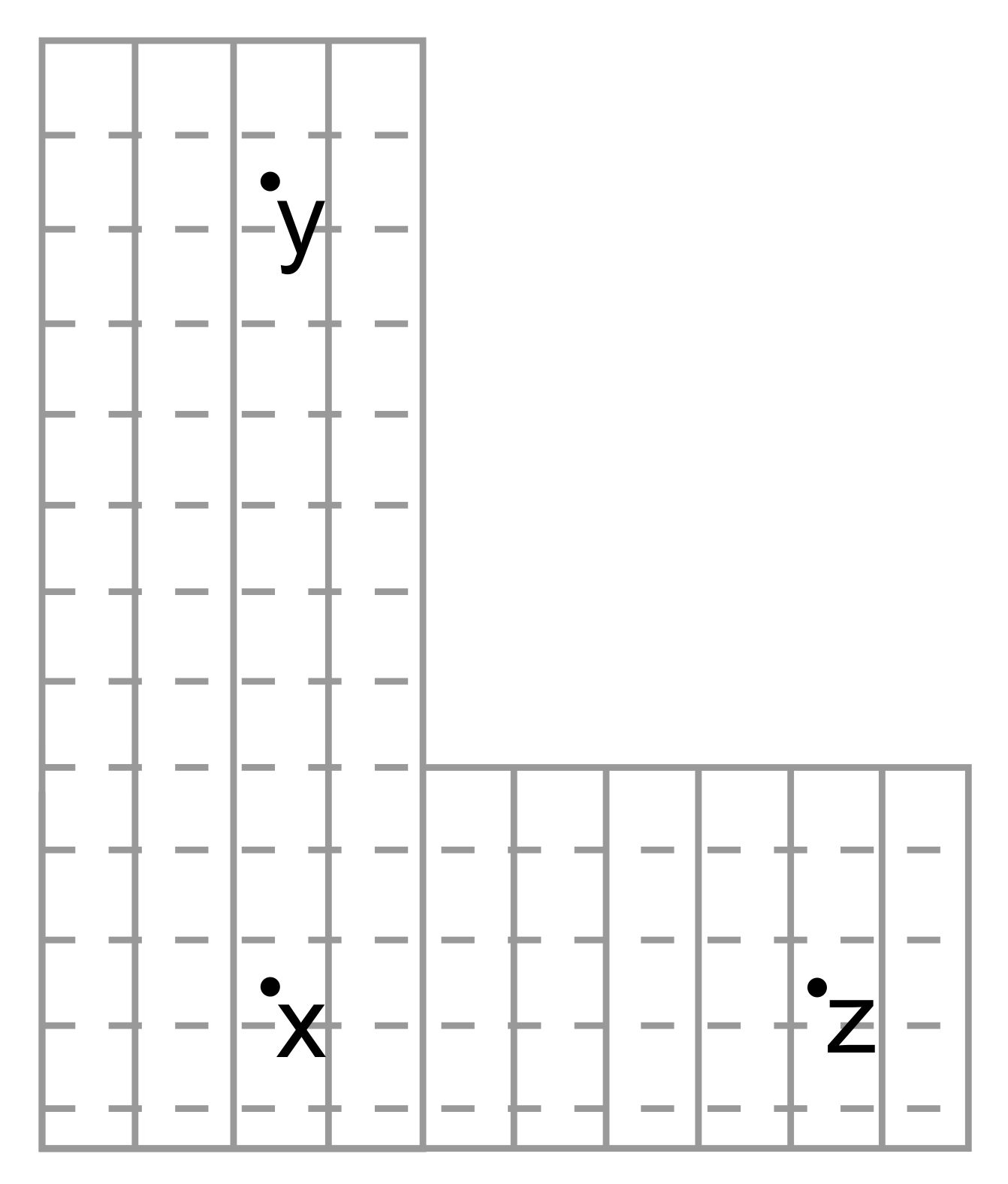
Figure 2: $\mathcal{A}(x)\neq\mathcal{A}(z)$.

Naturally, if a diffeormorfism $\phi$ is such that for some $x\in M$, we have that $\phi(x)\not\in\mathcal{A}(x)$ then $\phi$ is not decomposable in a neighbourhood of $x$.

2.2 Dynamical obstruction

Next Proposition contains properties of the dynamics of the leaves along the components of a decomposable flow. These simple properties explain topologically the nondecomposability of some diffeomorphisms.

Proposition 2.4.

Suppose that $\varphi_{t}$ has the decomposition $\varphi_{t}=\xi_{t}\circ\psi_{t}$ up to a stopping time $\tau>0$ a.s.. Then, for $0\leq t<\tau$, $\psi_{t}(x)\in\mathcal{V}(x)\cap\mathcal{H}(\varphi_{t}(x))$ and $\xi_{t}(y)\in\mathcal{H}(y)\cap\varphi_{t}(\mathcal{V}(y))$ where $x$ and $y$ are in the appropriate domain.

Proof.

The first statement follows easily from the fact that $\psi_{t}(x)\in\mathcal{V}(x)$ and $\xi_{t}$ preserves the horizontal leaves. The second statement follows obviously from the fact that $\xi_{t}(y)\in\mathcal{H}(y)$ and $y\in\mathcal{V}(y)$.

∎

Consider the plane $\mathbf{R}^{2}$ endowed with the usual vertical and horizontal foliations. A rotation by $\pi/2$ does not satisfy the second property of Proposition 2.4. Hence dynamical obstruction is independent of attainability since $\mathcal{A}(p)=\mathbf{R}^{2}$ for all $p\in\mathbf{R}^{2}$.

2.3 Preserving transverse orientation

Suppose that the horizontal foliation is transversely orientable and fix a biregular atlas with positive transverse orientation for the horizontal foliation. Given a continuous family $\phi_{t}$ of (global) diffeomorphisms on $M$ with $\phi_{0}=1d$ and a point $p\in M$, consider two local coordinate systems in this atlas: $\eta_{p}:U_{p}\subset M\rightarrow\mathbf{R}^{n-k}\times\mathbf{R}^{k}$, in a neighbourhood of $p$ and $\eta_{\phi_{t}(p)}:U_{\phi_{t}(p)}\subset M\rightarrow\mathbf{R}^{n-k}\times\mathbf{R}^{k}$, in a neighbourhood of $\phi_{t}(p)$. With respect to these coordinate systems one writes the family of diffeomorphisms locally as $\phi_{t}=(\phi_{t}^{1}(x,y),\phi_{t}^{2}(x,y))$, such that

$${\begin{array}[]{c}{{}_{n-k+1,\ldots,n}}\\ \mathrm{det}\\ {{}^{n-k+1,...,n}}\end{array}}D\phi_{t}(x)=\det\frac{\partial\phi_{t}^{2}(x,y)}{\partial y},$$ (2)

where the determinant above is taken for the $k\times k$ submatrices defined by the intersections of the columns indicated by subscripts and rows indicated by the superscripts. Distinct choices of coordinate systems in this atlas does not change the sign of the determinant above. Globally we have the following results whose main application is when $\phi_{t}$ is a flow of diffeomorphisms.

Theorem 2.5.

Suppose that the foliations $(M,\mathcal{H},\mathcal{V})$ is transversely orientable for the horizontal foliation. Let $(\phi_{t})_{t\in[0,a)}$ be a family of diffeomorphisms on $M$ depending continuously on $t$, with $\phi_{0}=1d$. The family of diffeomorphisms $\phi_{t}$ is globally decomposable for all $t\in[0,a)$ if and only if it preserves the transverse orientation, i.e.

$${\begin{array}[]{c}{{}_{n-k+1,...,n}}\\ \mathrm{det}\\ {{}^{n-k+1,...,n}}\end{array}}D\phi_{t}(x)>0,$$

for any $x\in M$ and for all $t\in[0,a)$.

Proof.

The idea of the proof is to show that if the global decomposition exists up to a time $t_{0}<a$, then the decomposition can be extended to $t_{0}+\delta$, with a positive $\delta$. This construction involves changing of local charts which are horizontal and vertically compatible with each other. These coherent local charts are paving the next $\delta$-time future trajectories as the system evolves.

For each $p\in M$, take a bounded open set $U_{p}$ which belongs to the biregular atlas. Define $t_{0}=\sup\{t\in[0,a):\phi_{t}|_{U_{p}}\mbox{ is decomposable as }\phi_{t}=\xi_{t}\circ\psi_{t}\}$. Suppose that $t_{0}<a$. Initially we prove that $\phi_{t_{0}}$ is locally decomposable. Since $p$ and $\phi_{t_{0}}(p)$ might be in distinct local chart, Proposition 1.4 does not apply directly.

For each $t<t_{0}$, we claim that there exist three coordinate systems $((x_{\alpha},y_{\alpha}),U_{\alpha})$, $\alpha=1,2$ or 3, covering $p$, $\psi_{t}(p)$ and $\phi_{t}(x)$, respectively, defined on open sets $U_{p},U_{\psi(p)}$ and $U_{\phi(p)}$ which are coherent in $\mathbf{R}^{n}$ in the sense that, distinct points in the same horizontal leaf have the same $y_{\alpha}$ coordinate; analogously to the vertical leaves. Precisely (omitting the subscript $t$):

• If $u\in U_{p}$ and $v\in U_{\psi(p)}$ with $\mathcal{V}(u)=\mathcal{V}(v)$ then $x_{p}(u)=x_{\psi(p)}(v);$

• If $u\in U_{\psi(p)}$ e $v\in U_{\phi(p)}$ with $\mathcal{H}(u)=\mathcal{H}(v)$ then $y_{\psi(p)}(u)=y_{\phi(p)}(v)$.

In fact, using that there exists a biregular coordinate system $\eta_{\psi(p)}:U_{\psi(p)}\rightarrow\mathbf{R}^{n}$ in a neighbourhood of $\psi(p)$, consider $\eta_{p}=\eta_{\psi(p)}\circ\psi_{p}$ and $\eta_{\phi(p)}=\eta_{\psi(p)}\circ\xi^{-1}$. With this choice of local coordinates, properties (i) and (ii) above follow directly from the fact that $\psi$ preserves leaves of $\mathcal{V}$ and $\xi$ preserves leaves of $\mathcal{H}$.

By continuity of $\phi_{t}$ we have that for each $q\in U_{p}$ there exists an $\epsilon>0$, sufficiently small, such that $\phi_{t_{0}}(q)$ is attainable from $U_{p}$ at time $(t_{0}-\epsilon)$, i.e. $\phi_{t_{0}}(q)\in\phi_{t_{0}-\epsilon}(U_{p})$. Consider the local diffeomorphism on $\mathbf{R}^{n}$ given by

$$\tilde{\phi}_{q}:=\eta_{\phi(p)}\circ\phi_{t_{0}}\circ\eta^{-1}_{p},$$

where the coherent coordinate systems $\eta_{\phi(p)}$ and $\eta_{p}$ above refer to time $(t_{0}-\epsilon)$. By hypothesis

$${\begin{array}[]{c}{{}_{n-k+1,...,n}}\\ \mathrm{det}\\ {{}^{n-k+1,...,n}}\end{array}}(D\tilde{\phi}_{q})>0.$$

Therefore, by Proposition 1.4, $\tilde{\phi}_{q}$ has a unique decomposition $\tilde{\phi}_{q}=\tilde{\xi}_{q}\circ\tilde{\psi}_{q}$ in $\mathbf{R}^{n-k}\times\mathbf{R}^{k}$ such that the component $\tilde{\xi}_{q}$ preserves vertical coordinates and $\tilde{\psi}_{q}$ preserves horizontal coordinates. Take

$$\psi_{q}=\eta_{\psi(p)}^{-1}\circ\tilde{\psi}_{q}\circ\eta_{p}\ \ \ \mbox{ and }\ \ \ \xi_{q}=\eta_{\phi(p)}^{-1}\circ\tilde{\xi}_{q}\circ\eta_{\psi(p)}.$$

The uniqueness of the local decomposition and the coherency of the coordinate systems allow us to glue all the $\psi_{q}$, $q\in U_{p}$, together into a diffeomorphism $\psi_{p}$, defined all over $U_{p}$. Analogously, we construct the horizontal component $\xi_{p}$ defined all over $U_{\psi(p)}$. Then $\phi_{t_{0}}$ is decomposable in the neighbourhood $U_{p}$ of $p$, for all $p\in M$.

Now, suppose by contradiction that $t_{0}<a$. We are going to show that there exist a sufficiently small $\delta>0$ such that $\phi_{t_{0}+\delta}$ is also decomposable. This finishes the proof, since the converse is trivial. Since $U_{\psi(p)}$ is birregular (here the subscript $t_{0}$ is omitted), it can be restricted such that its image by $\eta_{\psi(p)}$ is an $n$-dimensional rectangle whose border $\partial{U_{\psi(p)}}$ of $U_{\psi(p)}$ is the union of purely horizontal components $\partial^{h}U_{\psi(p)}$ and purely vertical components $\partial^{v}U_{\psi(p)}$. In this case, the trajectory of $\psi_{t}(q)$, along the time $t$, leaves $U_{p}$, gets in and out of $U_{\psi(p)}$ only by crossing their horizontal borders.

By Theorem 1.2, the set $U_{\psi(p)}$ can be extended vertically to $U^{\prime}_{\psi(p)}$ (extending vertically in the neighbourhood of each point of the compact $\partial^{h}U_{\psi(p)}$). For the set $U_{\phi(p)}$, each point in the border $\partial U_{\phi(p)}$ has either a horizontal or a vertical leaf crossing the border $\partial U_{\phi(p)}$ at this point. Then, again, by Theorem 1.2, this set can be enlarged to an open set $U^{\prime}_{\phi(p)}$ which contains the original one in its interior. Hence, the coordinate charts in the sets $U^{\prime}_{\psi(p)}$ and $U^{\prime}_{\phi(p)}$ are still coherent. So that, for $\delta>0$ sufficiently small, $\phi_{t_{0}+\delta}(U_{p})\subset U^{\prime}_{\phi(p)}$. This allows the decomposition to be performed at $t_{0}+\delta$. We conclude that $t_{0}=a$.

Finally, the global result is obtained using that at any point $p\in M$, the decomposition of $\phi_{t}|_{U_{p}}$, in a neighbourhood $U_{p}$ of $p$ holds for all $t\in[0,a)$. Using the uniqueness of local decomposition (Proposition 1.4) in the intersections of the neighbourhoods $U_{p}$, for all $p\in M$, we obtain the global decomposition for all $t\in[0,a)$.

∎

Transverse orientation in the proof above is crucial to guarantee that the sign of $\det_{n-k+1,...,n}^{n-k+1,...,n}D\phi_{t}$ is globally defined.

Corollary 2.6.

Suppose that the foliations $(M,\mathcal{H},\mathcal{V})$ is transversely orientable for the horizontal foliation. Given $x\in M$, if $\varphi_{t}(x)$ approaches the boundary $\partial\mathcal{A}(x)$ of the attainable set, then the subdeterminant goes to zero.

Proof.

Suppose that there exists $x\in M$ and $t_{0}>0$ such that $\varphi_{t_{0}}(x)\in\partial\mathcal{A}(x)$. Then $\phi_{t_{0}}$ is not decomposable. Therefore $\mbox{det}^{n-k+1,...,n}_{n-k+1,...,n}(D\phi_{t_{0}}(x))=0$ by Theorem 2.5.

∎

The foliations in figure 1 illustrates the result stated in this corollary. The horizontal foliation is transversely orientable. Hence, any flow which carries an $x_{0}$ to the boundary $\partial\mathcal{A}(x_{0})$ has the subdeterminant going to zero as it approaches $\partial\mathcal{A}(x_{0})$.

Example 2.7.

Theorem above states conditions for decomposability in transversely orientable horizontal foliation. Consider the quotient manifold $M=[0,1]^{3}/\sim$ where the projection is taken under the identification of two faces of the cube:

$$(x,0,z)\sim(1-x,1,1-z)$$

such that the leave $(x,y,1/2)$ turns into a Möbius strip $S$. Hence $M$ is a tubular neighbourhood of this Möbius strip with horizontal foliation $\mathcal{H}$ given by the image of the horizontal plaques and vertical foliation $\mathcal{V}$ is the corresponding image of the vertical lines. Although $(M,\mathcal{H})$ is not transversely orientable, the connected foliated space $(M\setminus S,\mathcal{H})$ is transversely orientable.

Consider the complete flow given by the projection of $\varphi_{t}(x,y,z)=(x,y+t,z)$. With respect to this pair of foliation, $\varphi_{t}$ is a horizontal flow, hence we have a trivial decomposition $\varphi_{t}=\xi_{t}\circ\psi_{t}$ given by $\xi_{t}=\varphi_{t}$ and $\psi_{t}\equiv Id$ for small $t$. When we consider the non-transversely orientable foliation $(M,\mathcal{H})$, for a local biregular chart in a neighbourhood of an initial condition $x_{0}\in S$, just before times $t\in\{(2k+1)2\pi,\mbox{ with }k\in\mathbf{Z}\}$ the decomposition does not exists as continuous trajectories in the subgroups of diffeomorphisms: since $\varphi_{t}$ reverses simultaneously the orientation of both the vertical and horizontal leaves passing through $x_{0}$, before any of these times, the decomposition $\varphi_{t}=\xi_{t}\circ\psi_{t}$ breaks continuity: it is given by the projection of the two reverting orientation diffeomorphisms $\xi_{t}(x,y,z)=(y,x,z)$ and $\psi_{t}(x,y,z)=(x,y,1-z)$. However, in the manifold $(M\setminus S,\mathcal{H})$ the decomposition is guaranteed by Theorem 2.5 for all $t\geq 0$.

3 Linear algebra of subdeterminants

In this section, we obtain an Itô formula for the subdeterminants in expression (2) for the linearised solutions of Stratonovich SDE. With this formula we obtain sufficient conditions for the decomposition of stochastic flows for all $t\geq 0$. Initially, we present some basic results on linear algebra, including the well-known Cauchy-Binet formula for the determinant of a product of matrices.

Lemma 3.1.

Let $A,B:\mathbf{R}^{n-k}\oplus\mathbf{R}^{k}\rightarrow\mathbf{R}^{n-k}\oplus\mathbf{R}^{k}$ be linear isomorphisms which are block diagonals preserving the subspaces $\mathbf{R}^{n-k}\times\{0\}$ and $\{0\}\times\mathbf{R}^{k}$. Then, for any linear operator $Y$ in $\mathbf{R}^{n}$, the subdeterminant

$${\begin{array}[]{c}{{}_{n-k+1,...,n}}\\ \mathrm{det}\\ {{}^{n-k+1,...,n}}\end{array}}(A\cdot Y\cdot B^{-1})=\left[{\begin{array}[]{c}{{}_{n-k+1,...,n}}\\ \mathrm{det}\\ {{}^{n-k+1,...,n}}\end{array}}(Y)\right]\left[{\begin{array}[]{c}{{}_{n-k+1,...,n}}\\ \mathrm{det}\\ {{}^{n-k+1,...,n}}\end{array}}(A\cdot B^{-1})\right].$$

Proof.

Straightforward using block matrices.

∎

This lemma guarantees that the concept of preserving transverse orientation diffeomorfism is well defined in terms of subdeterminants since it is independent of the local coordinate sistem in a transversely oriented atlas.

In general, given a $k\times n$ real matrix $C$, with $k,n\in\mathbf{N}$, we denote by $C_{j_{1}...j_{r}}$ the $k\times r$ submatrix obtained by selecting the $r\leq n$ columns ${j_{1}...j_{r}}$ from the original matrix $C$. Analogously, $C^{i_{1}...i_{r}}$, with $r\leq k$, represents the $r\times n$ submatrix obtained by selecting the $r$ rows ${i_{1},\ldots,i_{r}}$; yet the square matrix $C_{j_{1}...j_{r}}^{i_{1}...i_{r}}$, with $r\leq\min\{k,n\}$ is obtained by selecting the indicated rows and columns. The selection of rows commutes with the selection of columns. With this notation $\det(C)^{j_{1}...j_{r}}_{i_{1}...i_{r}}=\det C^{j_{1}...j_{r}}_{i_{1}...i_{r}}$. We use Cauchy-Binet formula to find an alternative expression of the Itô formula for the subdeterminants:

Lemma 3.2 (Cauchy-Binet).

Let $A$ be an $(l\times m)$-matrix and $B$ an $(m\times l)$-matrix, with $l\leq m$. Then,

$$\det(A\,B)=\sum_{i_{1}<i_{2}<...<i_{l}}\det({A}_{i_{1}...i_{l}})\cdot\det({B}^{i_{1}...i_{l}}).$$

For a proof, see e.g., among many others, Tracy and Widom [21].

3.1 Itô-Liouville Formula for subdeterminants

Consider initially that the Stratonovich SDE (1) takes place in an Euclidean space $\mathbf{R}^{n}$ with the associated stochastic flow of local diffeomorphisms $\varphi_{t}$. For equations in a Riemaninan manifold, using local coordinates, the results hold, up to the corresponging exit stopping times. Consider the linearized flow $Y_{t}=D\varphi_{t}:\mathbf{R}^{n}\rightarrow\mathbf{R}^{n}$, which satisfies:

$$dY_{t}=[DX_{0}(x_{t})]Y_{t}\ dt+\sum_{r=1}^{m}[DX_{r}(x_{t})]Y_{t}\circ dW^{r}_{t}.$$ (3)

where $DX_{r}$ are the derivative matrices of the corresponding vector fields relative to the canonical basis (covariant derivative $\nabla$, respectively, in a Riemannian manifold).

We use the following notation: given two $n\times n$ matrices $A$ and $B$, denote by $[A:B:j]$, with $1\leq j\leq n$, the matrix obtained by replacing the $j$-th row of $A$ by the the $j$-th row of $B$. Hence, for example

$$[I_{n}:DX_{i}:j]=\left(\begin{array}[]{ccc}I_{j-1}&&0\\ &&\\ \displaystyle\frac{\partial}{\partial x_{1}}X_{i}^{j}&\ldots&\displaystyle\frac{\partial}{\partial x_{n}}X^{j}_{i}\\ &&\\ 0&&I_{n-j-1}\end{array}\right),$$ (4)

where ‘0’ above represents zero submatrices with appropriate dimensions. We also recall the Laplace formula for the derivatives of the subdeterminants:

$$\frac{\partial}{\partial x_{i_{p}j_{q}}}{\begin{array}[]{c}{{}_{i_{1},\ldots,i_{k}}}\\ \mathrm{det}\\ {{}^{j_{1},\ldots,j_{k}}}\end{array}}(C)=(-1)^{p+q}{\begin{array}[]{c}{{}_{i_{1},...,\widehat{i_{p}},\ldots,i_{k}}}\\ \mathrm{det}\\ {{}^{j_{1},...,\widehat{j_{q}},\ldots,j_{k}}}\end{array}}(C),$$ (5)

with $1\leq p,q\leq k$, where the symbols $\widehat{i_{p}},\widehat{j_{q}}$ mean that these terms have been excluded.

Theorem 3.3.

For fixed $k$ rows $(i_{1},\ldots,i_{k})$ and $k$ columns $(j_{1},\ldots,j_{k})$, in the domain of existence of the stochastic flow of local diffeomorphism, we have the following Itô formula for the corresponding subdeterminant of the linearized flow:

$$\begin{array}[]{ccl}{\begin{array}[]{c}{{}_{i_{1}...i_{k}}}\\ \mathrm{det}\\ {{}^{j_{1}...j_{k}}}\end{array}}(Y_{t})&=&{\begin{array}[]{c}{{}_{i_{1}...i_{k}}}\\ \mathrm{det}\\ {{}^{j_{1}...j_{k}}}\end{array}}(I_{n})\ +\ \displaystyle\sum_{p=1}^{k}\int_{0}^{t}{\begin{array}[]{c}{{}_{i_{1}...i_{k}}}\\ \mathrm{det}\\ {{}^{j_{1}...j_{k}}}\end{array}}[Y_{s}:(DX_{0})\cdot Y_{s}:i_{p}]\ ds\\ &&\\ &&+\displaystyle\sum_{r=1}^{m}\ \displaystyle\sum_{p=1}^{k}\int_{0}^{t}{\begin{array}[]{c}{{}_{i_{1}...i_{k}}}\\ \mathrm{det}\\ {{}^{j_{1}...j_{k}}}\end{array}}[Y_{s}:(DX_{r})\cdot Y_{s}:i_{p}]\circ dW^{r}_{s}.\end{array}$$ (6)

Proof.

For sake of notation, use $G(C):=\det^{i_{1}...i_{k}}_{j_{1}...j_{k}}(C)$ where $C$ is an $n\times n$ real valued matrix. Applying Itô formula, we have that:

$$G(Y_{t})=G(I)+\displaystyle\sum_{p,q\leq k}\int_{0}^{t}\frac{\partial}{\partial x_{i_{p}j_{q}}}G(Y_{s})\circ dY_{i_{p}j_{q}}(s).$$ (7)

In coordinates, for all $1\leq i,j\leq n$, equation (3) leads to:

$$dY_{ij}(t)=\displaystyle\sum_{l=1}^{n}\displaystyle\frac{\partial}{\partial x_{l}}X^{i}_{0}(x_{t})Y_{lj}(t)\ dt+\sum_{r=1}^{m}\ \sum_{l=1}^{n}\frac{\partial}{\partial x_{l}}X_{r}^{i}(x_{t})Y_{lj}(t)\circ dW^{r}_{t}.$$ (8)

From Equations (7) and (8) we have that

$$\begin{array}[]{ll}G(Y_{t})=&G(I)+\displaystyle\sum_{l=1}^{n}\sum_{p,q\leq k}\int_{0}^{t}\frac{\partial}{\partial x_{i_{p}j_{q}}}G(Y_{s})\ \frac{\partial}{\partial x_{l}}X^{i_{p}}_{0}(x_{s})Y_{lj_{p}}(s)\ ds\\ &\\ &+\displaystyle\sum_{r=1}^{m}\ \sum_{l=1}^{n}\sum_{p,q\leq k}\int_{0}^{t}\frac{\partial}{\partial x_{i_{p}j_{q}}}G(Y_{s})\ \frac{\partial}{\partial x_{l}}X^{i_{p}}_{r}(x_{s})Y_{lj_{p}}(s)\circ dW^{r}_{s}.\end{array}$$

By Laplace formula (5), we have that

$$G([Y_{s}:(DX_{r})\cdot Y_{s}:i_{p}])=\sum_{q\leq k}\frac{\partial}{\partial x_{i_{p}j_{q}}}G(Y_{t})\ \sum_{l=1}^{n}\frac{\partial X_{r}^{i_{p}}}{\partial x_{l}}(x_{t})Y_{lj_{q}}.$$

Hence formula (6) of the statement follows.

∎

In particular, for the maximal subdeterminant, i.e. with $k=n$, one recovers the Liouville formula for determinants since for all $r$ in $\{0,1,\ldots,m\}$ we have that

$$\sum_{p=1}^{n}{\begin{array}[]{c}{{}_{i_{1},...,i_{n}}}\\ \mathrm{det}\\ {{}^{j_{1},...,j_{n}}}\end{array}}[Y_{s}:(DX_{r})\cdot Y_{s}:i_{p}]=\det(Y_{s})\cdot\mathrm{Tr}(DX_{r})\ \mathrm{sgn}(i)\ \mathrm{sgn}(j),$$

where $\mathrm{sgn}(i)$ and $\mathrm{sgn}(j)$ are the parities of the permutations $(i_{1},...,i_{n})$ and $(j_{1},...,j_{n})$, respectively.

Corollary 3.4.

For fixed $k$ rows $(i_{1},\ldots,i_{k})$ and $k$ columns $(j_{1},\ldots,j_{k})$, in the domain of existence of the stochastic flow of local diffeomorphism, we have the following Itô formula for the corresponding subdeterminant of the linearized flow:

$$\begin{array}[]{ccl}{\begin{array}[]{c}{{}_{i_{1}...i_{k}}}\\ \mathrm{det}\\ {{}^{j_{1}...j_{k}}}\end{array}}(Y_{t})&=&{\begin{array}[]{c}{{}_{i_{1}...i_{k}}}\\ \mathrm{det}\\ {{}^{j_{1}...j_{k}}}\end{array}}(I_{n})\ +\displaystyle\sum_{l_{1}<...<l_{k}}\ \displaystyle\sum_{p=1}^{k}\int_{0}^{t}{\begin{array}[]{c}{{}_{i_{1}...i_{k}}}\\ \mathrm{det}\\ {{}^{l_{1}..l_{k}}}\end{array}}[I:DX_{0}:i_{p}]\cdot{\begin{array}[]{c}{{}_{l_{1}...l_{k}}}\\ \mathrm{det}\\ {{}^{j_{1}...j_{k}}}\end{array}}(Y_{s})\ ds\\ &&\\ &&+\displaystyle\sum_{r=1}^{m}\ \displaystyle\sum_{l_{1}<...<l_{k}}\ \displaystyle\sum_{p=1}^{k}\int_{0}^{t}{\begin{array}[]{c}{{}_{i_{1}...i_{k}}}\\ \mathrm{det}\\ {{}^{l_{1}...l_{k}}}\end{array}}[I:DX_{r}:i_{p}]\cdot{\begin{array}[]{c}{{}_{l_{1}...l_{k}}}\\ \mathrm{det}\\ {{}^{j_{1}...j_{k}}}\end{array}}(Y_{s})\circ dW^{r}_{s}.\end{array}$$ (9)

Proof.

For each $i_{p}$, $1\leq p\leq k$ we have that

$$[Y_{s}:DX_{r}\cdot Y_{s}:i_{p}]=[I:DX_{r}:i_{p}]\cdot Y_{s}.$$

Then, apply Cauchy-Binet formula, Lemma (3.2), to each product $[I:DX_{i}:j]\cdot Y_{s}$.

∎

In this article we are particularly interested on applying formulae (6) and (9) for the subdeterminant of the lower–right $k\times k$ submatrices of $Y_{t}$, cf. Proposition 1.4 and Theorem 2.5.

3.2 Applications on decomposition of flows

Suppose that a Riemannian manifold $M$ is endowed with a horizontal foliation which is transversely orientable and assume that the stochastic flow $\varphi_{t}$ is complete. Theorem 2.5 says that the global decomposition of the stochastic flow $\varphi_{t}$ is determined by the subdeterminant $\det_{n-k+1,...,n}^{n-k+1,...,n}(D\varphi_{t})$, with respect to a biregular positively tranversal orientable coordinate system. Corollary 3.4 states that this subdeterminant can be written in terms of products of simpler subdeterminants. In our application here, if some of these subdeterminants vanish, then the equation for the relevant subdeterminant is a linear SDE, cf. Proposition 3.5 below. The geometrical meanings are given after the proposition. We have the following sufficient condition on the subdeterminants for the existence of global decomposition for all $t\geq 0$:

Proposition 3.5.

Assume that the $(M,\mathcal{H},\mathcal{V})$ is transversely orientable for the horizontal foliation. Suppose that for all $0\leq r\leq m$ we have that

$${\begin{array}[]{c}{{}_{n-k+1,...,n}}\\ \mathrm{det}\\ {{}^{l_{1},...,l_{k}}}\end{array}}[I:DX_{r}:i]\cdot{\begin{array}[]{c}{{}_{l_{1},...,l_{k}}}\\ \mathrm{det}\\ {{}^{n-k+1,...,n}}\end{array}}(Y_{t})=0,$$ (10)

for all $(n-k+1)\leq i\leq n$, all $(l_{1}>...>l_{k})$ except possibly $(l_{1},...,l_{k})=(n-k+1,\ldots,n)$ and all $t\geq 0$. Then $\varphi_{t}$ is decomposable for all $t\geq 0.$

Proof.

The hypotesis (10) together with the fact that $\varphi_{0}=Id$ implies that equation (9) reduces to

$$\begin{array}[]{ll}{\begin{array}[]{c}{{}_{n-k+1,...,n}}\\ \mathrm{det}\\ {{}^{n-k+1,...,n}}\end{array}}(Y_{t})=&1+\displaystyle\sum_{i=n-k+1}^{n}\int_{0}^{t}{\begin{array}[]{c}{{}_{n-k+1,\ldots,n}}\\ \mathrm{det}\\ {{}^{n-k+1,...,n}}\end{array}}([I:\nabla X_{0}:i]){\begin{array}[]{c}{{}_{n-k+1,...,n}}\\ \mathrm{det}\\ {{}^{n-k+1,...,n}}\end{array}}(Y_{s})\ ds\\ &+\displaystyle\sum_{r=1}^{m}\ \sum_{i=n-k+1}^{n}\int_{0}^{t}{\begin{array}[]{c}{{}_{n-k+1,\ldots,n}}\\ \mathrm{det}\\ {{}^{n-k+1,...,n}}\end{array}}([I:\nabla X_{r}:i]){\begin{array}[]{c}{{}_{n-k+1,...,n}}\\ \mathrm{det}\\ {{}^{n-k+1,...,n}}\end{array}}(Y_{s})\circ dW^{r}_{s}\end{array}$$

Therefore $\det_{n-k+1,...,n}^{n-k+1,\ldots,n}(Y_{t})$ is the solution of a linear SDE, with nonzero initial condition, hence, it never vanishes. The result follows by Theorem (2.5).

∎

Corollary 3.6.

If the stochastic flow $\varphi_{t}$ satisfies $\varphi_{t}(\mathcal{V}(p))\subset\mathcal{V}(\varphi_{t}(p))$ for all $p\in M$ then $\varphi_{t}$ is decomposable globally for all $t\geq 0$.

Proof.

In fact, in this case, $\frac{\partial\varphi_{t}^{i}}{\partial x_{j}}=0$ for all $n-k+1\leq j\leq n$ and $1\leq i\leq n-k$, hence

$${\begin{array}[]{c}{{}_{l_{1},...,l_{k}}}\\ \mathrm{det}\\ {{}^{n-k+1,...,n}}\end{array}}(Y_{t})=0,$$

for all $(l_{1}>...>l_{k})$ except $(l_{1},...,l_{k})=(n-k+1,\ldots,n)$. The result follows by the proposition above.

∎

The corollary above is illustrated by linear systems in $\mathbf{R}^{n}\setminus\{0\}$ with the spherical and radial foliations as the horizontal and vertical coordinates, respectively (cf. comments by the end of Prop. 1.4).

Corollary 3.7.

If the covariant derivative $\nabla_{v}X_{r}$ is horizontal for any direction $v\in TM$, for all $0\leq r\leq n$ then $\varphi_{t}$ is decomposable globally for all $t\geq 0$.

Proof.

In fact, in this case,

$${\begin{array}[]{c}{{}_{n-k+1,...,n}}\\ \mathrm{det}\\ {{}^{l_{1},...,l_{k}}}\end{array}}[I:DX_{r}:i]=0,$$

for all $(n-k+1)\leq i\leq n$, for all $(l_{1}>...>l_{k})$ including $(l_{1},...,l_{k})=(n-k+1,\ldots,n)$ and all $t\geq 0$. Then

$${\begin{array}[]{c}{{}_{n-k+1,...,n}}\\ \mathrm{det}\\ {{}^{n-k+1,...,n}}\end{array}}(Y_{t})\equiv 1,$$

The result follows by Proposition 3.5.

∎

References

- [1] J. M. Bismut – Mécanique aléatoire, Lecture Notes in Math., 866. Springer-Verlag, Berlin-New York, 1981.
- [2] C. Camacho and A. Lins Neto – Geometric theory of foliations. Birkhäuser Boston, 1985.
- [3] A. Candel and L. Conlon – Foliations I. Graduate Studies in Mathematics AMS, vol. 23. Providence, 1999.
- [4] P. J. Catuogno, F. B. da Silva and P. R. Ruffino – Decomposition of stochastic flows with automorphism of subbundles component. Stochastics and Dynamics 12 (2012), no. 2, 1150013, 15 pp.
- [5] P. J. Catuogno, F. B. da Silva and P. R. Ruffino – Decomposition of stochastic flows in manifolds with complementary distributions. Stochastics and Dynamics 13 (2013), no. 4, 1350009, 12 pp.
- [6] F. Colonius and P. R. Ruffino – Nonlinear Iwasawa decomposition of control flows. Discrete Continuous Dyn. Systems, (Serie A) Vol. 18 (2) p. 339-354, 2007.
- [7] K. D. Elworthy – Stochastic Differential equations on Manifolds, London Mathematical Society Lecture Note Series, 70. Cambridge University Press, 1982.
- [8] I. G. Gargate and P. R. Ruffino – An averaging principle for diffusions in foliated spaces. To appear in Annals of Probab. 2015.
- [9] H. Kunita – Stochastic differential equations and stochastic flows of diffeomorphisms, in: École d’Eté de Probabilités de Saint-Flour XII - 1982, ed. P.L. Hennequin, pp. 143–303. Lecture Notes on Maths. 1097 (Springer,1984).
- [10] H. Kunita – Stochastic flows and stochastic differential equations, Cambridge University Press, 1988.
- [11] X.-M. Li – An averaging principle for a completely integrable stochastic Hamiltonian system. Nonlinearity 21 (2008), no. 4, 803-822.
- [12] T. Kurtz, E. Pardoux and P. Protter – Stratonovich stochastic differential equations driven by general semimartingales. Annales de l’I.H.P., section B, tome 31, n. 2, 1995. p. 351-377.
- [13] M. Liao – Decomposition of stochastic flows and Lyapunov exponents, Probab. Theory Rel. Fields 117 (2000) 589-607.
- [14] A. M. Melo, L. B. Morgado and P. R. Ruffino – Decomposition of stochastic flows generated by Stratonovich SDEs with jumps. 2015 Arxiv. 1504.06562.
- [15] L. Morgado and P. Ruffino – Extension of time for decomposition of stochastic flows in spaces with complementary foliations. Electron. Comm. Probab., vol. 20 (2015), no. 38.
- [16] J. Milnor - Remarks on infinite dimensional Lie groups. In: Relativity, Groups and Topology II, Les Houches Session XL, 1983. North Holland, Amsterdam, 1984.
- [17] K.-H. Neeb - Infinite Dimesional Lie Groups. Monastir Summer Schoool, 2009. Available from hal.archives-ouvertes.fr/docs/00/39/…/CoursKarl-HermannNeeb.pdf
- [18] H. Omori - Infinite dimensional Lie groups. Translations of Math Monographs 158, AMS, 1997.
- [19] P. Ruffino – Decomposition of stochastic flow and rotation matrix. Stochastics and Dynamics, Vol. 2 (2002) 93-108.
- [20] I. Tamura - Topology of Foliations: An Introduction. Translations of AMS, vol. 97, 1992.
- [21] C. Tracy and H. Widom – On the distributions of the lengths of the longest monotone subsequences in random words. Probab. Theory and Related Fields, 119, pp. 350-380 (2001).
- [22] P. Walcak – Dynamics of foliations, groups and pseudogroups. Birkhäuser Verlag 2004.