Equivalence Checking By Logic Relaxation

Abstract

We introduce a new framework for Equivalence Checking (EC) of Boolean circuits based on a general technique called Logic Relaxation (LoR). The essence of LoR is to relax the formula to be solved and compute a superset $S$ of the set of new behaviors. Namely, $S$ contains all new satisfying assignments that appeared due to relaxation and does not contain assignments satisfying the original formula. Set $S$ is generated by a procedure called partial quantifier elimination. If all possible bad behaviors are in $S$, the original formula cannot have them and so the property described by this formula holds. The appeal of EC by LoR is twofold. First, it facilitates generation of powerful inductive proofs. Second, proving inequivalence comes down to checking the presence of some bad behaviors in the relaxed formula i.e. in a simpler version of the original formula. We give experimental evidence that supports our approach.

1 Introduction

1.1 Motivation

Our motivation for this work is threefold. First, Equivalence Checking (EC) is a crucial part of hardware verification. Second, more efficient EC enables more powerful logic synthesis transformations and so strongly impacts design quality. Third, intuitively, there should exist robust and efficient EC methods meant for combinational circuits computing values in a “similar manner”. Once discovered, these methods can be extended to EC of sequential circuits and even software.

1.2 Structural similarity of circuits

In this paper, we target EC of structurally similar circuits $N^{\prime}$ and $N^{\prime\prime}$. Providing a comprehensive definition of structural similarity is a tall order. Instead, below we give an example of circuits that can be viewed as structurally similar. Let $v^{\prime}$ be a variable of circuit $N^{\prime}$. Let $S(v^{\prime})=\mbox{$\{v^{\prime\prime}_{i_{1}},\dots,v^{\prime\prime}_{i_{k}}\}$}$ be a set of variables of $N^{\prime\prime}$ that have the following property. The knowledge of values assigned to the variables of $S(v^{\prime})$ in $N^{\prime\prime}$ under input $x$ is sufficient to find out the value of $v^{\prime}$ in $N^{\prime}$ under the same input $x$. (This means that $v^{\prime}$ is a function of variables of $S(v^{\prime})$ modulo assignments to $S(v^{\prime})$ that cannot be produced in $N^{\prime\prime}$ under any input.) Suppose that for every variable $v^{\prime}$ of $N^{\prime}$ there exists a small set $S(v^{\prime})$ with the property above. Then one can consider circuits $N^{\prime}$ and $N^{\prime\prime}$ as structurally similar. The smaller sets $S(v^{\prime})$, the closer $N^{\prime}$ and $N^{\prime\prime}$ structurally. In particular, if $N^{\prime}$ and $N^{\prime\prime}$ are identical, for every variable $v^{\prime}$ there is a set $S(v^{\prime})$ consisting only of one variable of $N^{\prime\prime}$. An example of structurally similar circuits where $S(v^{\prime})$ consists of two variables is given in Subsection 7.2.

1.3 EC by logic relaxation

Let $N^{\prime}(X^{\prime},Y^{\prime},z^{\prime})$ and $N^{\prime\prime}(X^{\prime\prime},Y^{\prime\prime},z^{\prime\prime})$ be single-output circuits to be checked for equivalence. Here $X^{\prime}$ and $Y^{\prime}$ specify the sets of input and internal variables of $N^{\prime}$ respectively and $z^{\prime}$ specifies the output variable of $N^{\prime}$. The same applies to $X^{\prime\prime},Y^{\prime\prime},z^{\prime\prime}$ of circuit $N^{\prime\prime}$. A traditional way to verify the equivalence of $N^{\prime}$ and $N^{\prime\prime}$ is to form a two-output circuit shown in Fig. 1 and check if $z^{\prime}\neq z^{\prime\prime}$ for some input assignment ($x^{\prime}$,$x^{\prime\prime}$) where $x^{\prime}$=$x^{\prime\prime}$. Here $x^{\prime}$ and $x^{\prime\prime}$ are assignments to variables of $X^{\prime}$ and $X^{\prime\prime}$ respectively. (By saying that $p$ is an assignment to a set of variables $V$, we will assume that $p$ is a complete assignment unless otherwise stated. That is every variable of $V$ is assigned a value in $p$.)

Formula $\mathit{EQ}(X^{\prime},X^{\prime\prime})$ relating inputs of $N^{\prime}$ and $N^{\prime\prime}$ in Fig. 1 evaluates to 1 for assignments $x^{\prime}$ and $x^{\prime\prime}$ to $X^{\prime}$ and $X^{\prime\prime}$ iff $x^{\prime}$=$x^{\prime\prime}$. (Usually, $N^{\prime}$ and $N^{\prime\prime}$ are just assumed to share the same set of input variables. In this paper, for the sake of convenience, we let $N^{\prime}$ and $N^{\prime\prime}$ have separate sets of input variables but assume that $N^{\prime}$ and $N^{\prime\prime}$ must be equivalent only for the input assignments satisfying $\mathit{EQ}(X^{\prime},X^{\prime\prime})$.)

EC by Logic Relaxation (LoR) presented in this paper is based on the following idea. Let $\mathit{Out}(N^{\prime},N^{\prime\prime})$ denote the set of outputs of $N^{\prime}$ and $N^{\prime\prime}$ when their input variables are constrained by $\mathit{EQ}(X^{\prime},X^{\prime\prime})$. For equivalent circuits $N^{\prime}$ and $N^{\prime\prime}$ that are not constants, $\mathit{Out}(N^{\prime},N^{\prime\prime})$ is equal to $\{(z^{\prime}=0,z^{\prime\prime}=0),(z^{\prime}=1,z^{\prime\prime}=1)\}$. Let $\mbox{$\mathit{Out}^{\mathit{rlx}}$}(N^{\prime},N^{\prime\prime})$ denote the set of outputs of $N^{\prime}$ and $N^{\prime\prime}$ when their inputs are not constrained by $\mathit{EQ}(X^{\prime},X^{\prime\prime})$ . (Here $\mathit{rlx}$ stands for “relaxed”). $\mbox{$\mathit{Out}^{\mathit{rlx}}$}(N^{\prime},N^{\prime\prime})$ is a superset of $\mathit{Out}(N^{\prime},N^{\prime\prime})$ that may contain an output $(z^{\prime}=0,z^{\prime\prime}=1)$ and/or output $(z^{\prime}=1,z^{\prime\prime}=0)$ even when $N^{\prime}$ and $N^{\prime\prime}$ are equivalent. Let $\mathit{D}_{\mathit{out}}$ denote $\mbox{$\mathit{Out}^{\mathit{rlx}}$}(N^{\prime},N^{\prime\prime})\setminus\mathit{Out}(N^{\prime},N^{\prime\prime})$. That is $\mathit{D}_{\mathit{out}}$ contains the outputs that can be produced only when inputs of $N^{\prime}$ and $N^{\prime\prime}$ are independent of each other.

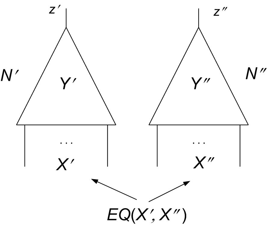
Figure 1: Equivalence checking of $N^{\prime}$ and $N^{\prime\prime}$

Computing set $\mathit{D}_{\mathit{out}}$ either solves the equivalence checking of $N^{\prime}$ and $N^{\prime\prime}$ or dramatically simplifies it. (This is important because, arguably, set $\mathit{D}_{\mathit{out}}$ is much easier to find than $\mathit{Out}(N^{\prime},N^{\prime\prime})$.) Indeed, assume that $\mathit{D}_{\mathit{out}}$ contains both $(z^{\prime}=1,z^{\prime\prime}=0)$ and $(z^{\prime}=0,z^{\prime\prime}=1)$. Then $N^{\prime}$ and $N^{\prime\prime}$ are equivalent because assignments where values of $z^{\prime}$ and $z^{\prime\prime}$ are different are present in $\mbox{$\mathit{Out}^{\mathit{rlx}}$}(N^{\prime},N^{\prime\prime})$ but not in $\mathit{Out}(N^{\prime},N^{\prime\prime})$. Now, assume that $\mathit{D}_{\mathit{out}}$ does not contain, say, assignment $(z^{\prime}=1,z^{\prime\prime}=0)$. This can only occur in the following two cases. First, $N^{\prime}$ cannot produce output 1 (i.e. $N^{\prime}$ is a constant 0) and/or $N^{\prime\prime}$ cannot produce 0 (i.e. $N^{\prime\prime}$ is a constant 1). Second, both $\mbox{$\mathit{Out}^{\mathit{rlx}}$}(N^{\prime},N^{\prime\prime})$ and $\mathit{Out}(N^{\prime},N^{\prime\prime})$ contain assignment $(z^{\prime}=1,z^{\prime\prime}=0)$ and hence $N^{\prime}$ and $N^{\prime\prime}$ are inequivalent. Separating these two cases comes down to checking if $N^{\prime}$ and $N^{\prime\prime}$ can evaluate to 1 and 0 respectively. If the latter is true, $N^{\prime}$ and $N^{\prime\prime}$ are inequivalent.

Set $\mathit{D}_{\mathit{out}}$ is built in EC by LoR by computing a sequence of so-called boundary formulas $H_{0},\dots,H_{k}$. Formula $H_{i}$ depends only on the variables of a cut of $N^{\prime},N^{\prime\prime}$ (see Figure 2) and excludes the assignments of $\mbox{$\mathit{D}_{\mathit{Cut}}$}_{i}=\mbox{$\mathit{Cut}_{i}^{\mathit{rlx}}$}(N^{\prime},N^{\prime\prime})\setminus\mathit{Cut}_{i}(N^{\prime},N^{\prime\prime})$. (That is every assignment of $\mbox{$\mathit{D}_{\mathit{Cut}}$}_{i}$ falsifies $H_{i}$). Here $\mbox{$\mathit{Cut}_{i}^{\mathit{rlx}}$}(N^{\prime},N^{\prime\prime})$ and $\mathit{Cut}_{i}(N^{\prime},N^{\prime\prime})$ are the sets of all cut assignments produced when inputs of $N^{\prime}$ and $N^{\prime\prime}$ are unconstrained or constrained by $\mathit{EQ}(X^{\prime},X^{\prime\prime})$ respectively. Formula $H_{0}$ is specified in terms of cut $X^{\prime}\cup X^{\prime\prime}$ and is equal to $EQ(X^{\prime},X^{\prime\prime})$. Formula $H_{k}$ is computed in terms of cut $\{z^{\prime},z^{\prime\prime}\}$ and so specifies the required set $\mathit{D}_{\mathit{out}}$ (as a set of assignments falsifying $H_{k}$). Boundary formulas are computed by a technique called partial quantifier elimination (PQE) introduced in [9]. In PQE, only a part of the formula is taken out of the scope of quantifiers. So PQE can be dramatically more efficient than complete quantifier elimination.

1.4 The appeal of EC by LoR

The appeal of EC by LoR is twofold. First, EC by LoR facilitates generation of very robust proofs by induction via construction of boundary formulas. By contrast, the current approaches (see e.g. [10, 11, 16]) employ fragile induction proofs e.g. those that require existence of functionally equivalent internal points. The size of boundary formulas depends on the similarity of $N^{\prime}$ and $N^{\prime\prime}$ rather than their individual complexity. This suggests that proofs of equivalence in EC by LoR can be generated efficiently.

Figure 2: Building boundary formula $\mathit{H}_{\mathit{cut}}$

Second, the machinery of boundary formulas facilitates proving inequivalence. Let $\mbox{$\mathit{F}_{\mathit{N^{\prime}}}$}(X^{\prime},Y^{\prime},z^{\prime})$ and $\mbox{$\mathit{F}_{\mathit{N^{\prime\prime}}}$}(X^{\prime\prime},Y^{\prime\prime},z^{\prime\prime})$ be formulas specifying $N^{\prime}$ and $N^{\prime\prime}$ respectively. (We will say that a Boolean formula $F_{N}$ specifies circuit $N$ if every assignment satisfying $F_{N}$ is a consistent assignment to variables of $N$ and vice versa. We will assume that all formulas mentioned in this paper are Boolean formulas in Conjunctive Normal Form (CNF) unless otherwise stated.)

Circuits $N^{\prime}$ and $N^{\prime\prime}$ are inequivalent iff formula $\mathit{EQ}(X^{\prime},X^{\prime\prime})\wedge F_{N^{\prime}}\wedge F_{N^{\prime\prime}}\wedge(z^{\prime}\not\equiv z^{\prime\prime})$ is satisfiable. Denote this formula as $\alpha$. As we show in this paper, $\alpha$ is equisatisfiable with formula $\beta$ equal to $\mbox{$\mathit{H}_{\mathit{cut}}$}\wedge F_{N^{\prime}}\wedge F_{N^{\prime\prime}}\wedge(z^{\prime}\not\equiv z^{\prime\prime})$. Here $\mathit{H}_{\mathit{cut}}$ is a boundary formula computed with respect to a cut (see Fig. 2.) In general, formula $\beta$ is easier to satisfy than $\alpha$ for the following reason. Let $p$ be an assignment satisfying formula $\beta$ . Let $x^{\prime}$ and $x^{\prime\prime}$ be the assignments to variables of $X^{\prime}$ and $X^{\prime\prime}$ respectively specified by $p$. Since variables of $X^{\prime}$ and $X^{\prime\prime}$ are independent of each other in formula $\beta$, in general, ${\mbox{\boldmath$x^{\prime}$}}\neq{\mbox{\boldmath$x^{\prime\prime}$}}$ and so $p$ does not satisfy $\alpha$. Hence, neither $x^{\prime}$ nor $x^{\prime\prime}$ are a counterexample. They are just inputs producing cut assignments $q^{\prime}$ and $q^{\prime\prime}$ (see Fig. 2) such that a) $\mbox{$\mathit{H}_{\mathit{cut}}$}({\mbox{\boldmath$q^{\prime}$}},{\mbox{\boldmath$q^{\prime\prime}$}})=1$ and b) $N^{\prime}$ and $N^{\prime\prime}$ produce different outputs under cut assignment ($q^{\prime}$,$q^{\prime\prime}$). To turn $p$ into an assignment satisfying $\alpha$ one has to do extra work. Namely, one has to find assignments $x^{\prime}$ and $x^{\prime\prime}$ to $X^{\prime}$ and $X^{\prime\prime}$ that are equal to each other and under which $N^{\prime}$ and $N^{\prime\prime}$ produce cut assignments $q^{\prime}$ and $q^{\prime\prime}$ above. Then $x^{\prime}$ and $x^{\prime\prime}$ specify a counterexample. So the equisatisfiability of $\alpha$ and $\beta$ allows one to prove $N^{\prime}$ and $N^{\prime\prime}$ inequivalent (by showing that $\beta$ is satisfiable) without providing a counterexample.

1.5 Contributions and structure of the paper

Our contributions are as follows. First, we present a new method of EC based on LoR meant for a very general class of structurally similar circuits. This method is formulated in terms of a new technique called PQE that is a “light” version of quantifier elimination. Showing the potential of PQE for building new verification algorithms is our second contribution. Third, we relate EC by LoR to existing methods based on finding equivalent internal points. In particular, we show that a set of clauses relating points of an equivalence cut of $N^{\prime}$ and $N^{\prime\prime}$ is a boundary formula. So boundary formulas can be viewed as a machinery for generalization of the notion of an equivalence cut. Fourth, we give experimental evidence in support of EC by LoR. In particular, we employ an existing PQE algorithm whose performance can be drastically improved for solving non-trivial EC problems. Fifth, we show that interpolation is a special case of LoR (and interpolants are a special case of boundary formulas.) In particular, we demonstrate that by using LoR one can interpolate a “broken” implication. This extension of interpolation can be used for generation of short versions of counterexamples.

The structure of this paper is as follows. Section 2 discusses the challenge of proving EC by induction. In Section 3, we show the correctness of EC by LoR and relate the latter to partial quantifier elimination. Boundary formulas are discussed in Section 4. Section 5 presents an algorithm of EC by LoR. Section 6 describes how one can apply EC by LoR if the power of a PQE solver is not sufficient to compute boundary formulas precisely. Section 7 provides experimental evidence in favor of our approach. In Section 8, some background is given. We relate interpolation and LoR in Section 9 and make conclusions in Section 10. The appendix of the paper contains six sections with additional information.

2 Proving Equivalence By Induction

Intuitively, for structurally similar circuits $N^{\prime}$ and $N^{\prime\prime}$, there should exist a short proof of equivalence shown in Fig. 3. In this proof, for every set $\mathit{Cut}_{i}$ forming a cut, only a small set $H_{i}$ of short clauses relating variables of $\mathit{Cut}_{i}$ is generated. (A clause is a disjunction of literals. We will use the notions of a CNF formula $C_{1}\wedge..\wedge C_{p}$ and the set of clauses $\{C_{1},\dots,C_{p}\}$ interchangeably). The relations of $i$-th cut specified by $H_{i}$ are derived using formulas $H_{j}$ built earlier i.e. $j<i$. This goes on until clauses specifying $z^{\prime}\equiv z^{\prime\prime}$ are derived. We will refer to the proof shown in Fig. 3 as a proof by induction (slightly abusing the term “induction”). A good scalability of the current EC tools is based on their ability to derive proofs by induction. However, they can find such proofs only when cut variables have a very tight relation (most commonly, an equivalence relation). This means that these tools can handle only a very narrow subclass of structurally similar circuits.

Proving EC by induction is a challenging task because one has to address the following cut termination problem. When does one stop generating a set of clauses $H_{i}$ in terms of variables of $\mathit{Cut}_{i}$ and switch to building formula $H_{i+1}$ relating variables of $\mathit{Cut}_{i+1}$? Let $M_{i}$ denote the subcircuit consisting of the gates of $N^{\prime}$ and $N^{\prime\prime}$ located below $i$-th cut (like subcircuit $M$ of Fig. 4). A straightforward way to build an inductive proof is to make formula $H_{i}$ specify the range of $M_{i}$ i.e. the set of all output assignments that can be produced by $M_{i}$. (We will also refer to the range of circuit $M_{i}$ as a cut image because it specifies all assignments that can appear on $i$-th cut.) Then formula $H_{i+1}$ can be derived from formula $H_{i}$ and the clauses specifying the gates located between $\mathit{Cut}_{i}$ and $\mathit{Cut}_{i+1}$. A flaw of this approach is that a formula specifying the image of $i$-th cut can get prohibitively large.

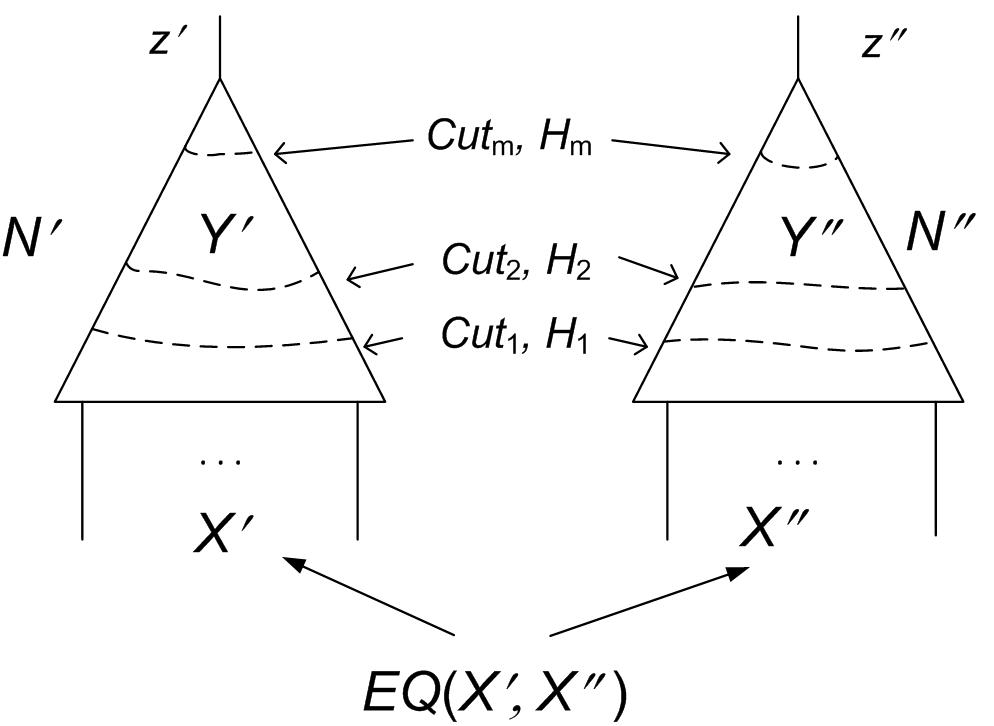
Figure 3: An inductive proof of equivalence

A solution offered in EC by LoR is to use the boundary formulas introduced in Subsection 1.3 as formulas $H_{i}$. This solution has at least three nice qualities. First, boundary formulas have simple semantics. ($H_{i}$ excludes the assignments of $i$-th cut that can be produced when inputs of $N^{\prime}$ and $N^{\prime\prime}$ are independent of each other but cannot be produced when inputs are constrained by $\mathit{EQ}(X^{\prime},X^{\prime\prime})$.) Second, the size of a boundary formula depends on the structural similarity of circuits $N^{\prime}$ and $N^{\prime\prime}$ rather than their individual complexity. In other words, a boundary formula computed for a cut is drastically simpler than a formula specifying the image of this cut in $N^{\prime}$ and $N^{\prime\prime}$. Third, formula $H_{i}$ can be inductively derived from $H_{i-1}$, which gives an elegant solution to the cut termination problem. The construction of formula $H_{i}$ ends (and that of $H_{i+1}$ begins) when adding $H_{i}$ to some quantified formula containing $H_{i-1}$ makes the latter redundant.

3 Equivalence Checking By LoR And PQE

In this section, we prove the correctness of Equivalence Checking (EC) by Lo-gic Relaxation (LoR) and relate the latter to Partial Quantifier Elimination (PQE). Subsection 3.1 introduces PQE. In Subsection 3.2, we discuss proving equivalence/inequivalence in EC by LoR. Besides, we relate EC by LoR to PQE.

3.1 Complete and partial quantifier elimination

In this paper, by a quantified formula we mean one with existential quantifiers. Given a quantified formula $\exists{W}[A(V,W)]$, the problem of quantifier elimination is to find a quantifier-free formula $A^{*}(V)$ such that $A^{*}\equiv\mbox{$\exists{W}[A]$}$. Given a quantified formula $\exists{W}[A(V,W)\wedge B(V,W)]$, the problem of Partial Quantifier Elimination (PQE) is to find a quantifier-free formula $A^{*}(V)$ such that $\mbox{$\exists{W}[A\wedge B]$}\equiv A^{*}\wedge\mbox{$\exists{W}[B]$}$. Note that formula $B$ remains quantified (hence the name partial quantifier elimination). We will say that formula $A^{*}$ is obtained by taking $A$ out of the scope of quantifiers in $\exists{W}[A\wedge B]$. Importantly, there is a strong relation between PQE and the notion of redundancy of a subformula in a quantified formula. In particular, solving the PQE problem above comes down to finding $A^{*}(V)$ implied by $A\wedge B$ that makes $A$ redundant in $A^{*}\wedge\mbox{$\exists{W}[A\wedge B]$}$. Indeed, in this case, $\mbox{$\exists{W}[A\wedge B]$}\equiv A^{*}\wedge\mbox{$\exists{W}[A\wedge B]$}\equiv A^{*}\wedge\mbox{$\exists{W}[B]$}$.

Importantly, redundancy with respect to a quantified formula is much more powerful than that with respect to a quantifier-free one. For instance, if formula $F(V)$ is satisfiable, every clause of $F$ is redundant in formula $\exists{V}[F]$. On the other hand, a clause $C$ is redundant in a quantifier-free formula $F$ only if $C$ is implied by $F\setminus\mbox{$\{C\}$}$.

Let $G(V)$ be a formula implied by $B$. Then $\mbox{$\exists{W}[A\wedge B]$}\equiv A^{*}\wedge G\wedge\mbox{$\exists{W}[B]$}$ entails $\mbox{$\exists{W}[A\wedge B]$}\equiv A^{*}\wedge\mbox{$\exists{W}[B]$}$. In other words, clauses implied by the formula that remains quantified are noise and can be removed from a solution to the PQE problem. So when building $A^{*}$ by resolution it is sufficient to use only the resolvents that are descendants of clauses of $A$. For that reason, in the case formula $A$ is much smaller than $B$, PQE can be dramatically faster than complete quantifier elimination. Another way to contrast complete quantifier elimination with PQE is as follows. The former deals with a single formula and so, in a sense, has to cope with its absolute complexity. By contrast, PQE computes formula $A^{*}$ that specifies the “difference” between formulas $B$ and $A\wedge B$. So the efficiency of PQE depends on their relative complexity. This is important because no matter how high the individual complexity of $B$ and $A\wedge B$ is, their relative complexity can be quite manageable. In Section 0.B of the appendix we briefly describe an algorithm for PQE and recall some relevant results [7, 8, 9].

3.2 Proving equivalence/inequivalence by LoR

Proposition 1 below shows how one proves equivalence/inequivalence of circuits by LoR. Let formula $G$ denote $\mathit{EQ}\wedge\mbox{$\mathit{F}_{\mathit{N^{\prime}}}$}\wedge\mbox{$\mathit{F}_{\mathit{N^{\prime\prime}}}$}$ and formula $\mathit{G}^{\mathit{rlx}}$ denote $\mbox{$\mathit{F}_{\mathit{N^{\prime}}}$}\wedge\mbox{$\mathit{F}_{\mathit{N^{\prime\prime}}}$}$. Recall from Subsection 1.4 that $F_{N^{\prime}}(X^{\prime},Y^{\prime},z^{\prime})$ and $F_{N^{\prime\prime}}(X^{\prime\prime},Y^{\prime\prime},z^{\prime\prime})$ specify circuits $N^{\prime}$ and $N^{\prime\prime}$ respectively. Formula $\mathit{EQ}({\mbox{\boldmath$x^{\prime}$}},{\mbox{\boldmath$x^{\prime\prime}$}})$ evaluates to 1 iff $x^{\prime}$=$x^{\prime\prime}$ where $x^{\prime}$ and $x^{\prime\prime}$ are assignments to variables of $X^{\prime}$ and $X^{\prime\prime}$ respectively.

Proposition 1

Let $H(z^{\prime},z^{\prime\prime})$ be a formula such that $\mbox{$\exists{W}[\mathit{EQ}\wedge\mbox{$\mathit{G}^{\mathit{rlx}}$}]$}\equiv H\wedge\mbox{$\exists{W}[\mbox{$\mathit{G}^{\mathit{rlx}}$}]$}$ where $W=X^{\prime}\cup X^{\prime\prime}\cup Y^{\prime}\cup Y^{\prime\prime}$. Then formula $G\wedge(z^{\prime}\not\equiv z^{\prime\prime})$ is equisatisfiable with $H\wedge\mbox{$\mathit{G}^{\mathit{rlx}}$}\wedge(z^{\prime}\not\equiv z^{\prime\prime})$.

Note that finding formula $H(z^{\prime},z^{\prime\prime})$ of Proposition 1 reduces to taking formula $\mathit{EQ}$ out of the scope of quantifiers i.e. to solving the PQE problem. Proposition 1 implies that proving inequivalence of $N^{\prime}$ and $N^{\prime\prime}$ comes down to showing that formula $\mathit{G}^{\mathit{rlx}}$ is satisfiable under assignment $(z^{\prime}=b^{\prime},z^{\prime\prime}=b^{\prime\prime})$ (where $b^{\prime},b^{\prime\prime}\in\mbox{$\{0,1\}$}$) such that $b^{\prime}\neq b^{\prime\prime}$ and $H(b^{\prime},b^{\prime\prime})=1$. Recall that the input variables of $N^{\prime}$ and $N^{\prime\prime}$ are independent of each other in formula $\mathit{G}^{\mathit{rlx}}$. Hence the only situation where $\mathit{G}^{\mathit{rlx}}$ is unsatisfiable under $(z^{\prime}=b^{\prime},z^{\prime\prime}=b^{\prime\prime})$ is when $N^{\prime}$ is constant $\overline{b^{\prime}}$ and/or $N^{\prime\prime}$ is constant $\overline{b^{\prime\prime}}$. So the corollary below holds.

Corollary 1

If neither $N^{\prime}$ nor $N^{\prime\prime}$ are constants, they are equivalent iff $H(1,0)=H(0,1)=0$.

Reducing EC to an instance of PQE also provides valuable information when proving equivalence of $N^{\prime}$ and $N^{\prime\prime}$. Formula $\mathit{G}^{\mathit{rlx}}$ remains quantified in $\mbox{$\exists{W}[\mathit{EQ}\wedge\mbox{$\mathit{G}^{\mathit{rlx}}$}]$}\equiv H\wedge\mbox{$\exists{W}[\mbox{$\mathit{G}^{\mathit{rlx}}$}]$}$. This means that to obtain formula $H$, it suffices to generate only resolvents that are descendants of clauses of $\mathit{EQ}$. The clauses obtained by resolving solely clauses of $\mathit{G}^{\mathit{rlx}}$ are just “noise” (see Subsection 3.1). This observation is the basis for our algorithm of generating EC proofs by induction.

4 Boundary Formulas

In this section, we discuss boundary formulas, a key notion of EC by LoR. Subsection 4.1 explains the semantics of boundary formulas. Subsection 4.2 discusses the size of boundary formulas. In Subsection 4.3, we describe how boundary formulas are built.

4.1 Definition and some properties of boundary formulas

Let $M$ be the subcircuit consisting of the gates of $N^{\prime},N^{\prime\prime}$ located before a cut as shown in Fig. 4. As usual, $G$ denotes $\mathit{EQ}(X^{\prime},X^{\prime\prime})\wedge F_{N^{\prime}}\wedge F_{N^{\prime\prime}}$ and $\mathit{G}^{\mathit{rlx}}$ does $F_{N^{\prime}}\wedge F_{N^{\prime\prime}}$.

Definition 1

Let formula $\mathit{H}_{\mathit{cut}}$ depend only on variables of a cut. Let $q$ be an assignment to the variables of this cut. Formula $\mathit{H}_{\mathit{cut}}$ is called boundary if

1. $G\rightarrow\mbox{$\mathit{H}_{\mathit{cut}}$}$ holds and

2. for every $q$ that can be extended to satisfy $\mathit{G}^{\mathit{rlx}}$ but cannot be extended to satisfy $G$, the value of $\mathit{H}_{\mathit{cut}}$($q$) is 0.

Note that Definition 1 does not specify the value of $\mathit{H}_{\mathit{cut}}$($q$) if $q$ cannot be extended to satisfy $\mathit{G}^{\mathit{rlx}}$ (and hence $G$). As we mentioned in the introduction, formula $\mathit{EQ}(X^{\prime},X^{\prime\prime})$ and formula $H(z^{\prime},z^{\prime\prime})$ of Proposition 1 are actually boundary formulas with respect to cuts $X^{\prime}\cup X^{\prime\prime}$ and $\{z^{\prime},z^{\prime\prime}\}$ respectively. We will refer to $H(z^{\prime},z^{\prime\prime})$ as an output boundary formula. Proposition 2 below reduces building $\mathit{H}_{\mathit{cut}}$ to PQE.

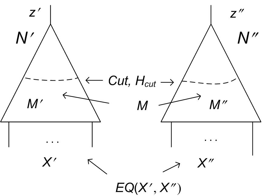
Figure 4: Building boundary formula $\mathit{H}_{\mathit{cut}}$

Proposition 2

Let $\mathit{H}_{\mathit{cut}}$ be a formula depending only on variables of a cut. Let $\mathit{H}_{\mathit{cut}}$ satisfy $\mbox{$\exists{W}[\mathit{EQ}\wedge F_{M}]$}\equiv\mbox{$\mathit{H}_{\mathit{cut}}$}\wedge\mbox{$\exists{W}[F_{M}]$}$. Here $W$ is the set of variables of $F_{M}$ minus those of the cut. Then $\mathit{H}_{\mathit{cut}}$ is a boundary formula.

Proposition 3 below extends Proposition 1 to an arbitrary boundary formula.

Proposition 3

Let $\mathit{H}_{\mathit{cut}}$ be a boundary formula with respect to a cut. Then $G\wedge(z^{\prime}\not\equiv z^{\prime\prime})$ is equisatisfiable with $\mbox{$\mathit{H}_{\mathit{cut}}$}\wedge\mbox{$\mathit{G}^{\mathit{rlx}}$}\wedge(z^{\prime}\not\equiv z^{\prime\prime})$.

The proposition below estimates the size of boundary formulas built for $N^{\prime}$ and $N^{\prime\prime}$ that satisfy the notion of structural similarity introduced in Subsection 1.2.

Proposition 4

Let $\mathit{Cut^{\prime}},\mathit{Cut}^{\prime\prime}$ specify the outputs of circuits $M^{\prime}$ and $M^{\prime\prime}$ of Fig. 4 respectively. Assume that for every variable $v^{\prime}$ of $\mathit{Cut^{\prime}}$ there is a set $S(v^{\prime})=\mbox{$\{v^{\prime\prime}_{i_{1}},\dots,v^{\prime\prime}_{i_{k}}\}$}$ of variables of $\mathit{Cut^{\prime\prime}}$ that have the following property. Knowing the values of variables of $S(v^{\prime})$ produced in $N^{\prime\prime}$ under input $x$ one can determine the value of $v^{\prime}$ of $N^{\prime}$ under the same input $x$. We assume here that $S(v^{\prime})$ has this property for every possible input $x$. Let $\mathit{Max}(S(v^{\prime}))$ be the size of the largest $S(v^{\prime})$ over variables of $\mathit{Cut^{\prime}}$. Then there is a boundary formula $\mathit{H}_{\mathit{cut}}$ where every clause has at most $\mathit{Max}(S(v^{\prime}))+1$ literals.

Proposition 4 demonstrates the existence of small boundary formulas for structurally similar circuits $N^{\prime}$,$N^{\prime\prime}$. Importantly, the size of these boundary formulas depend on similarity of $N^{\prime}$ and $N^{\prime\prime}$ rather than their individual complexity.

Corollary 2

Let circuits $M^{\prime}$ and $M^{\prime\prime}$ of Fig. 4 be functionally equivalent. Then for every variable $v^{\prime}\in\mathit{Cut^{\prime}}$ there is a set $S(v^{\prime})=\mbox{$\{v^{\prime\prime}\}$}$ where $v^{\prime\prime}$ is the variable of $\mathit{Cut^{\prime\prime}}$ that is functionally equivalent to $v^{\prime}$. In this case, formula $\mathit{EQ}(\mathit{Cut}^{\prime},\mathit{Cut}^{\prime\prime})$ stating equivalence of corresponding output variables of $M^{\prime}$ and $M^{\prime\prime}$ is a boundary formula for the cut in question. This formula can be represented by $2\!*\!p$ two-literal clauses where $p=|Cut^{\prime}|=|Cut^{\prime\prime}|$.

Proposition 4 and the corollary above show that the machinery of boundary formulas allows one to extend the notion of an equivalence cut to the case where structurally similar circuits have no functionally equivalent internal variables.

4.2 Size of boundary formulas in general case

Proposition 4 above shows the existence of small boundary formulas for a particular notion of structural similarity. In this subsection, we make two observations that are applicable to a more general class of structurally similar circuits than the one outlined in Subsection 1.2.

The first observation is as follows. Let $q$ be an assignment to the cut of Fig. 4. Assignment $q$ can be represented as ($q^{\prime}$,$q^{\prime\prime}$) where $q^{\prime}$ and $q^{\prime\prime}$ are assignments to output variables of $M^{\prime}$ and $M^{\prime\prime}$ respectively. Definition 1 does not constrain the value of $\mathit{H}_{\mathit{cut}}$($q$) if $q$ cannot be extended to satisfy $F_{N^{\prime}}\wedge F_{N^{\prime\prime}}$. So, if, for instance, output $q^{\prime}$ cannot be produced by $M^{\prime}$ for any input, the value of $\mathit{H}_{\mathit{cut}}$($q$) can be arbitrary. This means that $\mathit{H}_{\mathit{cut}}$ does not have to tell apart cut assignments that can be produced by $M^{\prime}$ and $M^{\prime\prime}$ from those that cannot. In other words, $\mathit{H}_{\mathit{cut}}$ does not depend on the individual complexity of $M^{\prime}$ and $M^{\prime\prime}$. Formula $\mathit{H}_{\mathit{cut}}$ has only to differentiate cut assignments that can be produced solely when ${\mbox{\boldmath$x^{\prime}$}}\neq{\mbox{\boldmath$x^{\prime\prime}$}}$ from those that can be produced when $x^{\prime}$=$x^{\prime\prime}$. Here $x^{\prime}$ and $x^{\prime\prime}$ are assignments to $X^{\prime}$ and $X^{\prime\prime}$ respectively.

The second observation is as follows. Intuitively, even a very broad definition of structural similarity of $N^{\prime}$ and $N^{\prime\prime}$ implies the existence of many short clauses relating cut variables that can be derived from $\mathit{EQ}(X^{\prime},X^{\prime\prime})\wedge F_{M}$. These clauses can be effectively used to eliminate the output assignments of $M$ that can be produced only by inputs ($x^{\prime}$,$x^{\prime\prime}$) where ${\mbox{\boldmath$x^{\prime}$}}\neq{\mbox{\boldmath$x^{\prime\prime}$}}$. Proposition 4 above substantiates this intuition in case the similarity of $N^{\prime}$ and $N^{\prime\prime}$ is defined as in Subsection 1.2.

4.3 Computing Boundary Formulas

The key part of EC by LoR is to compute an output boundary formula $H(z^{\prime},z^{\prime\prime})$. In this subsection, we show how to build formula $H$ inductively by constructing a sequence of boundary formulas $H_{0},\dots,H_{k}$ computed with respect to cuts $\mathit{Cut}_{0},\dots,\mathit{Cut}_{k}$ of $N^{\prime}$ and $N^{\prime\prime}$ (see Fig. 3). We assume that $\mathit{Cut}_{0}=X^{\prime}\cup X^{\prime\prime}$ and $\mathit{Cut}_{k}=\mbox{$\{z^{\prime},z^{\prime\prime}\}$}$ (i.e. $H=H_{k}$) and $\mathit{Cut}_{i}\cap\mathit{Cut}_{j}=\emptyset$ if $i\neq j$.

Boundary formula $H_{0}$ is set to $\mathit{EQ}(X^{\prime},X^{\prime\prime})$ whereas formula $H_{i}$, $i>0$ is computed from $H_{i-1}$ as follows. Let $M_{i}$ be the circuit consisting of the gates located between the inputs of $N^{\prime}$ and $N^{\prime\prime}$ and cut $\mathit{Cut_{i}}$ (as circuit $M$ of Fig. 4). Let $F_{M_{i}}$ be the subformula of $\mathit{G}^{\mathit{rlx}}$ specifying $M_{i}$. Let $W_{i}$ consist of all the variables of $F_{M_{i}}$ minus those of $\mathit{Cut}_{i}$. Formula $H_{i}$ is built to satisfy $\mbox{$\exists{W_{i}}[H_{i-1}\wedge F_{M_{i}}]$}\equiv H_{i}\wedge\mbox{$\exists{W_{i}}[F_{M_{i}}]$}$ and so make the previous boundary formula $H_{i-1}$ redundant in $H_{i}\wedge\mbox{$\exists{W_{i}}[H_{i-1}\wedge F_{M_{i}}]$}$. The fact that $H_{1},\dots,H_{k}$ are indeed boundary formulas follows from Proposition 5.

Proposition 5

Let $W_{i}$ where $i>0$ be the set of variables of $F_{M_{i}}$ minus those of $\mathit{Cut}_{i}$. Let $H_{i-1}$ where $i>1$ be a boundary formula such that $\mbox{$\exists{W_{i-1}}[H_{0}\wedge F_{M_{i-1}}]$}\equiv H_{i-1}\wedge\exists{W_{i-1}}[F_{M_{i-1}}]$. Let $\mbox{$\exists{W_{i}}[H_{i-1}\wedge F_{M_{i}}]$}\equiv H_{i}\wedge\mbox{$\exists{W_{i}}[F_{M_{i}}]$}$ hold. Then $\exists{W_{i}}[H_{0}\wedge F_{M_{i}}]$ $\equiv$ $H_{i}\wedge\mbox{$\exists{W_{i}}[F_{M_{i}}]$}$ holds. (So $H_{i}$ is a boundary formula due to Proposition 2.)

5 Algorithm of EC by LoR

In this section, we introduce an algorithm called $\mathit{EC\!\_LoR}$ that checks for equivalence two single-output circuits $N^{\prime}$ and $N^{\prime\prime}$. The pseudo-code of $\mathit{EC\!\_LoR}$ is given in Figure 5. $\mathit{EC\!\_LoR}$ builds a sequence of boundary formulas $H_{0},\dots,H_{k}$ as described in Subsection 4.3. Here $H_{0}$ equals $\mathit{EQ}(X^{\prime},X^{\prime\prime})$ and $H_{k}(z^{\prime},z^{\prime\prime})$ is an output boundary formula. Then, according to Proposition 1, $\mathit{EC\!\_LoR}$ checks the satisfiability of formula $H_{k}\wedge\mbox{$\mathit{G}^{\mathit{rlx}}$}\wedge(z^{\prime}\not\equiv z^{\prime\prime})$ where $\mbox{$\mathit{G}^{\mathit{rlx}}$}=F_{N^{\prime}}\wedge F_{N^{\prime\prime}}$.

$\mathit{EC\!\_LoR}(N^{\prime},N^{\prime\prime})${
1	$(N^{\prime},N^{\prime\prime}):=\mathit{Bufferize}(N^{\prime},N^{\prime\prime})$;
2	$\mathit{Cut}_{0}=X^{\prime}\cup X^{\prime\prime}$;
3	$\mathit{Cut}_{k}:=\mbox{$\{z^{\prime},z^{\prime\prime}\}$}$;
4	$\mathit{Cut}_{1},..,\mathit{Cut}_{k-1}\!:=\!\mathit{BldCuts}(N^{\prime},N^{\prime\prime})$;
5	$H_{0}:=\mathit{EQ}(X^{\prime},X^{\prime\prime})$;
$----------------$
6	$\mathit{for}(i:=1;i\leq k;i\mathit{+\!+})$ {
7		$H_{i}=1$;
8		$F_{M_{i}}:=\mathit{SubForm}(\mbox{$\mathit{G}^{\mathit{rlx}}$},\mathit{Cut}_{i})$;
9		$W_{i}:=\mathit{Vars}(F_{M_{i}})\setminus\mathit{Vars}(\mathit{Cut}_{i})$;
10		while ($\mathit{true}$) {
11			$C\!:=\!Redund(H_{i}\!\wedge\!\mbox{$\exists{W_{i}}[H_{i-1}\!\wedge\!F_{M_{i}}]$})$;
12			if ($C=\mathit{nil}$) break;
13			$H_{i}:=H_{i}\wedge C$;}}
$----------------$
14	if ($H_{k}(0,1)=1$)
15		if $(Sat(\mbox{$\mathit{G}^{\mathit{rlx}}$}\wedge\overline{z^{\prime}}\wedge z^{\prime\prime}))$ return(No);
16	if ($H_{k}(1,0)=1$)
17		if $(Sat(\mbox{$\mathit{G}^{\mathit{rlx}}$}\wedge z^{\prime}\wedge\overline{z^{\prime\prime}}))$ return(No);
18	return(Yes); }

Figure 5: EC by LoR

$\mathit{EC\!\_LoR}$ consists of three parts separated by the dotted lines in Figure 5. $\mathit{EC\!\_LoR}$ starts the first part (lines 1-5) by calling procedure $\mathit{Bufferize}$ that eliminates non-local connections of $N^{\prime}$ and $N^{\prime\prime}$ i.e. those that span more than two consecutive topological levels. (The topological level of a gate $g$ of a circuit $K$ is the longest path from an input of $K$ to $g$ measured in the number of gates on this path.) The presence of non-local connections makes it hard to find cuts that do not overlap. To avoid this problem, procedure $\mathit{Bufferize}$ replaces every non-local connection spanning $d$ topological levels ($d>2$) with a chain of $d-2$ buffers. (A more detailed discussion of this topic is given in Section 0.C of the appendix.) Then $\mathit{EC\!\_LoR}$ sets the initial and final cuts to $X^{\prime}\cup X^{\prime\prime}$ and $\{z^{\prime},z^{\prime\prime}\}$ respectively and computes the intermediate cuts.

Boundary formulas $H_{i}$, $1\leq i\leq k$ are computed in the second part (lines 6-13) that consists of a for loop. In the third part (lines 14-18), $\mathit{EC\!\_LoR}$ uses the output boundary formula $H_{k}(z^{\prime},z^{\prime\prime})$ computed in the second part to decide whether $N^{\prime},N^{\prime\prime}$ are equivalent. If $H_{k}(b^{\prime},b^{\prime\prime})=1$ where $b^{\prime}\neq b^{\prime\prime}$ and $\mathit{G}^{\mathit{rlx}}$ is satisfiable under $z^{\prime}=b^{\prime},z^{\prime\prime}=b^{\prime\prime}$, then $N^{\prime},N^{\prime\prime}$ are inequivalent. Otherwise, they are equivalent (line 18).

Formula $H_{i}$ is computed as follows. First, $H_{i}$ is set to constant 1. Then, $\mathit{EC\!\_LoR}$ extracts a subformula $F_{M_{i}}$ of $\mathit{G}^{\mathit{rlx}}$ that specifies the gates of $N^{\prime}$ and $N^{\prime\prime}$ located between the inputs and cut $\mathit{Cut}_{i}$. $\mathit{EC\!\_LoR}$ also computes the set $W_{i}$ of quantified variables. The main work is done in a while loop (lines 10-13). First, $\mathit{EC\!\_LoR}$ calls procedure $\mathit{Redund}$ that is essentially a PQE-solver. $\mathit{Redund}$ checks if boundary formula $H_{i-1}$ is redundant in $H_{i}\wedge\mbox{$\exists{W_{i}}[H_{i-1}\wedge F_{M_{i}}]$}$ (the cut termination condition). $\mathit{Redund}$ stops as soon as it finds out that $H_{i-1}$ is not redundant yet. It returns a clause $C$ as the evidence that at least one clause must be added to $H_{i}$ to make $H_{i-1}$ redundant. If no clause is returned by $\mathit{Redund}$, then $H_{i}$ is complete and $\mathit{EC\!\_LoR}$ ends the while loop and starts a new iteration of the for loop. Otherwise, $\mathit{EC\!\_LoR}$ adds $C$ to $H_{i}$ and starts a new iteration of the while loop.

6 Computing Boundary Formulas By Current PQE Solvers

To obtain boundary formula $H_{i}$, one needs to take $H_{i-1}$ out of the scope of quantifiers in formula $\exists{W_{i}}[H_{i-1}\wedge F_{M_{i}}]$ whose size grows with $i$ due to formula $F_{M_{i}}$. So a PQE solver that computes $H_{i}$ must have good scalability. On the other hand, the algorithm of [9] does not scale well yet. The main problem here is that learned information is not re-used in contrast to SAT-solvers effectively re-using learned clauses. Fixing this problem requires some time because bookkeeping of a PQE algorithm is more complex than that of a SAT-solver (see the discussion in Sections 0.B and 0.E of the appendix.) In this section, we describe two methods of adapting EC by LoR to a PQE-solver that is not efficient enough to compute boundary formulas precisely. (Both methods are illustrated experimentally in Section 7.)

One way to reduce the complexity of computing $H_{i}$ is to use only a subset of $F_{M_{i}}$. For instance, one can discard the clauses of $F_{M_{i}}$ specifying the gates located between cuts $\mathit{Cut}_{0}$ and $\mathit{Cut}_{p}$, $0<p<i$. In this case, boundary formula $H_{i}$ is computed approximately. The downside of this is that condition b) of Definition 1 does not hold anymore and so EC by LoR becomes incomplete. Namely, if $H(b^{\prime},b^{\prime\prime})=1$ where $b^{\prime}\neq b^{\prime\prime}$, the fact that $\mathit{G}^{\mathit{rlx}}$ is satisfiable under $z^{\prime}=b^{\prime},z^{\prime\prime}=b^{\prime\prime}$ does not mean that $N^{\prime}$ and $N^{\prime\prime}$ are inequivalent. Nevertheless, even EC by LoR with approximate computation of boundary formulas can be a powerful tool for proving $N^{\prime}$ and $N^{\prime\prime}$ equivalent for the following reason. If $H(1,0)=H(0,1)=0$, circuits $N^{\prime}$ and $N^{\prime\prime}$ are proved equivalent no matter how intermediate boundary formulas have been built. Importantly, checking cut termination conditions is a powerful way to structure the proof even when boundary formulas are computed approximately. That is, construction of $H_{i}$ still ends when it makes $H_{i-1}$ redundant in formula $H_{i}\wedge\mbox{$\exists{W_{i}}[H_{i-1}\wedge F_{M_{i}}]$}$. The only difference from computing $H_{i}$ precisely is that formula $F_{M_{i}}$ is simplified by discarding some clauses.

Another way to adapt EC by LoR to an insufficiently efficient PQE solver is as follows. Suppose that the power of a PQE solver is enough to build one intermediate boundary formula $H_{i}$ precisely. From Proposition 3 it follows that formula $\alpha$ equal to $G\wedge(z^{\prime}\not\equiv z^{\prime\prime})$ is equisatisfiable with formula $\beta$ equal to $\mbox{$\mathit{H}_{\mathit{cut}}$}\wedge\mbox{$\mathit{G}^{\mathit{rlx}}$}\wedge(z^{\prime}\not\equiv z^{\prime\prime})$. So, to show that $N^{\prime}$ and $N^{\prime\prime}$ are inequivalent it is sufficient to find an assignment satisfying $\beta$. As we argued in Subsection 1.4, finding such an assignment for $\beta$ is easier than for $\alpha$.

7 Experiments

In the experiments, we used the PQE solver published in [9] in 2014. We will refer to this solver as PQE-14. As we mentioned in Section 6, PQE-14 does not scale well yet. So building a full-fledged equivalence checker based on $\mathit{EC\!\_LoR}$ would mean simultaneously designing a new EC algorithm and a new PQE solver. The latter is beyond the scope of our paper (although the design of an efficient PQE-solver is discussed in Section 0.B of the appendix). On the other hand, PQE-14 is efficient enough to make a few important points experimentally. In the experiments described in this section, we employed a new implementation of PQE-14.

The experiment of Subsection 7.1 compares computing cut image with building a boundary formula for this cut. (Recall that the image of a cut is the set of cut assignments that can be produced in $N^{\prime}$ and $N^{\prime\prime}$ under all possible inputs.) This experiment also contrasts complete quantifier elimination employed to compute cut image with PQE. In Subsection 7.2, we apply $\mathit{EC\!\_LoR}$ to a non-trivial instance of equivalence checking that is hard for ABC, a high-quality synthesis and verification tool [20]. In Subsection 7.3, we give evidence that boundary formulas can be used to prove inequivalence more efficiently.

In the experiments, circuits $N^{\prime}$ and $N^{\prime\prime}$ to be checked for equivalence were derived from a circuit computing an output median bit of a $k$-bit multiplier. We will refer to this circuit as $\mathit{Mlp}_{k}$. Our motivation here is as follows. In many cases, the equivalence of circuits with simple topology and low fanout values can be efficiently checked by a general-purpose SAT-solver. This is not true for circuits involving multipliers. In all experiments, circuits $N^{\prime}$ and $N^{\prime\prime}$ were bufferized to get rid of long connections (see Section 5).

7.1 Image computation versus building boundary formulas

Table 1: Computing cut image and boundary formula. Time limit = 1 hour

#bits	#quan.	#free	cut image		boundary for-
	vars	vars	(QE)		mula (PQE)
			result		result
			size	(s.)	size	(s.)
8	32	84	3,142	4.0	242	0.1
9	36	104	4,937	13	273	0.2
10	40	126	7,243	51	407	0.3
11	44	150	9,272	147	532	0.5
12	48	176	14,731	497	576	0.6
13	52	206	19,261	1,299	674	0.9
14	56	234	$*$	$*$	971	1.5
15	60	266	$*$	$*$	1,218	2.0
16	64	300	$*$	$*$	1,411	3.0

In this subsection, we compared computation of a boundary formula $\mathit{H}_{\mathit{cut}}$ and that of cut image. We used two identical copies of circuit $\mathit{Mlp}_{k}$ as circuits $N^{\prime}$ and $N^{\prime\prime}$. As a cut of $N^{\prime},N^{\prime\prime}$ we picked the set of variables of the first topological level (every variable of this level specifies the output of a gate fed by input variables of $N^{\prime}$ or $N^{\prime\prime}$). Computing cut image comes down to performing quantifier elimination for formula $\exists{W}[\mathit{EQ}(X^{\prime},X^{\prime\prime})\wedge F_{M}]$. Here $W=X^{\prime}\cup X^{\prime\prime}$ and formula $F_{M}$ specifies the gates of the first topological level of $N^{\prime}$ and $N^{\prime\prime}$. Formula $\mathit{R}_{\mathit{cut}}$ that is logically equivalent to $\exists{W}[\mathit{EQ}\wedge F_{M}]$ specifies the cut image. Computing a boundary formula comes down to finding $\mathit{H}_{\mathit{cut}}$ such that $\mbox{$\exists{W}[\mathit{EQ}\wedge F_{M}]$}\equiv\mbox{$\mathit{H}_{\mathit{cut}}$}\wedge\mbox{$\exists{W}[F_{M}]$}$ i.e. solving the PQE problem.

The results of the experiment are given in Table 1. Abbreviation QE stands for Quantifier Elimination. The value of $k$ in $\mathit{Mlp}_{k}$ is shown in the first column. The next two columns give the number of quantified and free variables in $\exists{W}[\mathit{EQ}\wedge F_{M}]$. To compute formula $\mathit{R}_{\mathit{cut}}$ above we used our quantifier elimination program presented in [8]. Formula $\mathit{H}_{\mathit{cut}}$ was generated by PQE-14. To make this comparison fair, formula $\mathit{H}_{\mathit{cut}}$ was computed without applying any EC-specific heuristics (as opposed to computing boundary formulas in the experiments of Subsection 7.2). When computing image formula $\mathit{R}_{\mathit{cut}}$ and boundary formula $\mathit{H}_{\mathit{cut}}$ we recorded the size of the result (as the number of clauses) and the run time in seconds. As Table 1 shows, formulas $\mathit{H}_{\mathit{cut}}$ are much smaller than $\mathit{R}_{\mathit{cut}}$ and take much less time to compute.

7.2 An example of equivalence checking by $\mathit{EC\!\_LoR}$ 

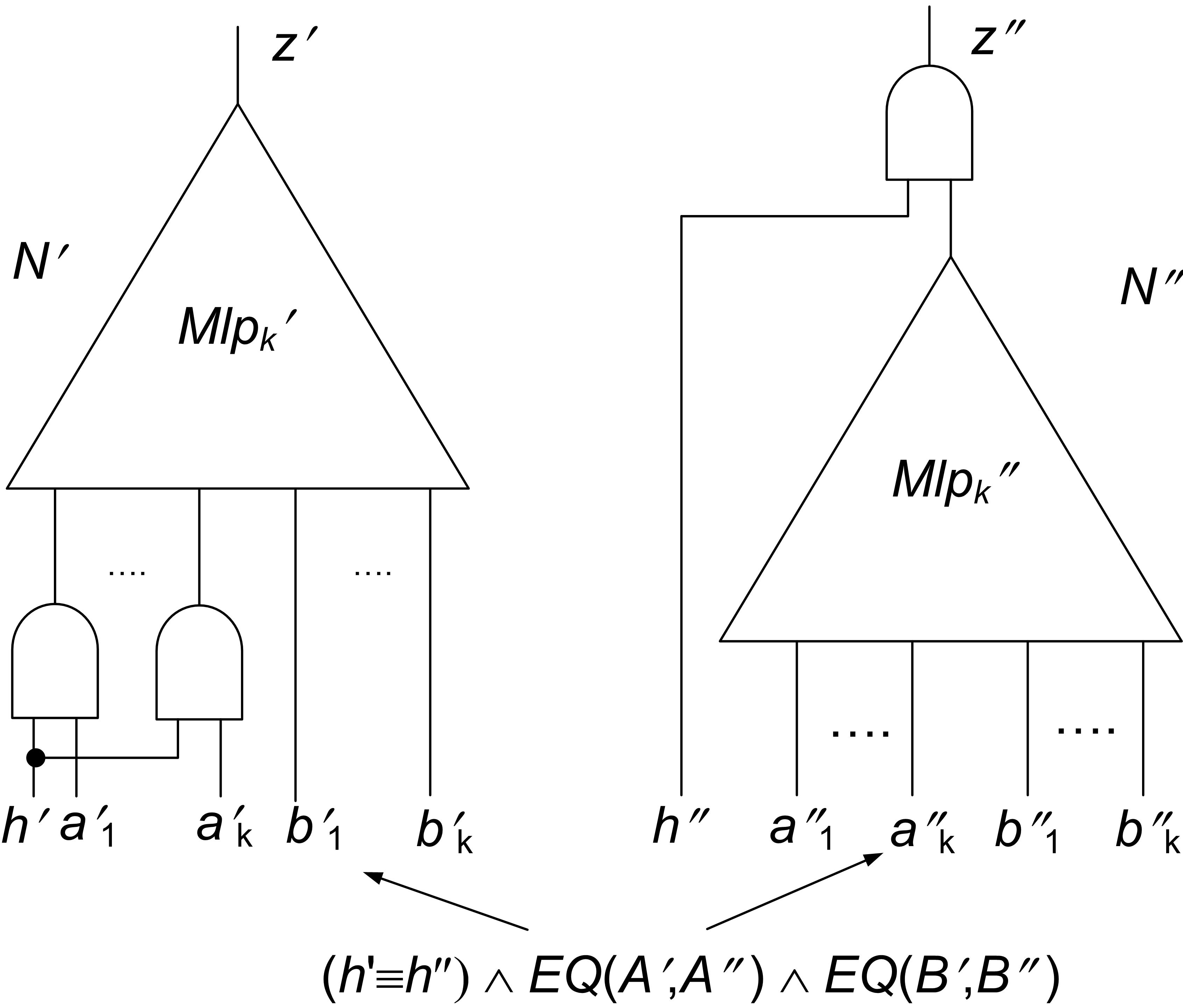
Figure 6: Equivalence checking of $N^{\prime}$ and $N^{\prime\prime}$ derived from $\mathit{Mlp}_{k}$

In this subsection, we run an implementation of $\mathit{EC\!\_LoR}$ introduced in Section 5 on circuits $N^{\prime}$ and $N^{\prime\prime}$ shown in Fig. 6. (The idea of this EC example was suggested by Vigyan Singhal [19].) These circuits are derived from $\mathit{Mlp}_{k}$ by adding one extra input $h$. Both circuits produce the same output as $\mathit{Mlp}_{k}$ when $h=1$ and output 0 if $h=0$. So $N^{\prime}$ and $N^{\prime\prime}$ are logically equivalent. Note that the value of every internal variable of $N^{\prime}$ depends on $h$ whereas this is not the case for $N^{\prime\prime}$. So $N^{\prime}$ and $N^{\prime\prime}$ have no functionally equivalent internal variables. On the other hand, $N^{\prime}$ and $N^{\prime\prime}$ satisfy the notion of structural similarity introduced in Subsection 1.2. Namely, the value of every internal variable $v^{\prime}$ of $N^{\prime}$ is specified by that of $h^{\prime\prime}$ and some variable $v^{\prime\prime}$ of $N^{\prime\prime}$ (So, in this case, for every internal variable $v^{\prime}$ of $N^{\prime}$ there is a set $S(v^{\prime})$ introduced in Subsection 1.2 consisting of only two variables of $N^{\prime\prime}$.). In particular, if $v^{\prime}$ is an internal variable of $\mathit{Mlp}_{k}^{\prime}$, then $v^{\prime\prime}$ is the corresponding variable of $\mathit{Mlp}_{k}^{\prime\prime}$. Indeed, if $h^{\prime\prime}=1$, then $v^{\prime}$ takes the same value as $v^{\prime\prime}$. If $h^{\prime\prime}=0$, then $v^{\prime}$ is a constant (in the implementation of $\mathit{Mlp}_{k}$ we used in the experiments). The objective of the experiment below is to show that $\mathit{EC\!\_LoR}$ can check for equivalence structurally similar circuits that have no functionally equivalent internal points.

Cuts $\mathit{Cut}_{0},\dots,\mathit{Cut}_{m}$ used by $\mathit{EC\!\_LoR}$ 
were generated according to topological levels. That is every variable of $\mathit{Cut}_{i}$ specified the output of a gate of $i$-th topological level. Since $N^{\prime}$ and $N^{\prime\prime}$ were bufferized, $\mathit{Cut}_{i}\cap\mathit{Cut}_{j}=\emptyset$ if $i\neq j$. The version of $\mathit{EC\!\_LoR}$ we used in the experiment was slightly different from the one described in Fig. 5. We will refer to this version as $\mathit{EC\!\_LoR}^{*}$. The main change was that boundary formulas were computed in $\mathit{EC\!\_LoR}^{*}$ approximately. That is when checking if formula $H_{j}$ was redundant in $H_{j}\wedge\mbox{$\exists{W_{i}}[H_{j-1}\wedge F_{M_{i}}]$}$ (line 11 of Fig. 5) only a subset of clauses of $F_{M_{i}}$ was used to make the check simpler. Nevertheless, $\mathit{EC\!\_LoR}^{*}$ was able to compute an output boundary formula $H(z^{\prime},z^{\prime\prime})$ proving that $N^{\prime}$ and $N^{\prime\prime}$ were equivalent. One more difference between $\mathit{EC\!\_LoR}$ and $\mathit{EC\!\_LoR}^{*}$ was as follows. $\mathit{EC\!\_LoR}$ runs a cut termination check every time formula $H_{i}$ is updated (in the while loop of Fig. 5, lines 10-13). In $\mathit{EC\!\_LoR}^{*}$, the number of cut termination checks was reduced. Namely, derivation of clauses of $H_{i}$ was modified so that $\mathit{EC\!\_LoR}^{*}$ did not run a cut termination check if some cut variable was not present in clauses of $H_{i}$ yet. The intuition here was that in that case $H_{i}$ was still under-constrained. $\mathit{EC\!\_LoR}^{*}$ is described in Section 0.D of the appendix in more detail.

Table 2: EC of $N^{\prime}$ and $N^{\prime\prime}$ derived from $\mathit{Mlp}_{k}$. Time limit = 6 hours

#bits	#vars	#clauses	#cuts	$\mathit{EC\!\_LoR}^{*}$	ABC
				(s.)	(s.)
10	2,844	6,907	37	4.5	10
11	3,708	8,932	41	7.1	38
12	4,726	11,297	45	11	142
13	5,910	14,026	49	16	757
14	7,272	17,143	53	25	3,667
15	8,824	20,672	57	40	11,237
16	10,578	24,637	61	70	$>$ 21,600

In Table 2, we compare $\mathit{EC\!\_LoR}^{*}$ 
with ABC [20]. The first column gives the value of $k$ of $\mathit{Mlp}_{k}$ used in $N^{\prime}$ and $N^{\prime\prime}$. The next two columns show the size of formulas $\mathit{EQ}(X^{\prime},X^{\prime\prime})\wedge F_{N^{\prime}}\wedge F_{N^{\prime\prime}}\wedge(z^{\prime}\not\equiv z^{\prime\prime})$ specifying equivalence checking of $N^{\prime}$ and $N^{\prime\prime}$ to which $\mathit{EC\!\_LoR}^{*}$ was applied. (Circuits $N^{\prime}$ and $N^{\prime\prime}$ were fed into ABC as circuits in the BLIF format.) Here $X=\mbox{$\{h,a_{1},\dots,a_{k},b_{1},\dots,b_{k}\}$}$ denotes the set of input variables. The fourth column shows the number of topological levels in circuits $N^{\prime}$ and $N^{\prime\prime}$ and so the number of cuts used by $\mathit{EC\!\_LoR}^{*}$. The last two columns give the run time of $\mathit{EC\!\_LoR}^{*}$ and ABC.

The results of Table 2 show that equivalence checking of $N^{\prime}$ and $N^{\prime\prime}$ derived from $\mathit{Mlp}_{k}$ was hard for ABC. On the other hand, $\mathit{EC\!\_LoR}^{*}$ managed to solve all instances in a reasonable time. Most of the run time of $\mathit{EC\!\_LoR}^{*}$ is taken by PQE-14 when checking cut termination conditions. So, PQE-14 is also the reason why the run time of $\mathit{EC\!\_LoR}^{*}$ grows quickly with the size of $\mathit{Mlp}_{k}$. Using a more efficient PQE-solver should reduce such a strong dependency of the performance of $\mathit{EC\!\_LoR}^{*}$ on the value of $k$.

7.3 Using boundary formulas for proving inequivalence

In the experiment of this subsection, we checked for equivalence a correct and a buggy version of $\mathit{Mlp}_{16}$ as circuits $N^{\prime}$ and $N^{\prime\prime}$ respectively. Since $\mathit{EC\!\_LoR}^{*}$ described in the previous subsection computes boundary formulas approximately, one cannot directly apply it to prove inequivalence of $N^{\prime}$ and $N^{\prime\prime}$. In this experiment we show that the precise computation of even one boundary formula corresponding to an intermediate cut can be quite useful for proving inequivalence. Let $\alpha$ and $\beta$ denote formulas $\mathit{EQ}(X^{\prime},X^{\prime\prime})\wedge F_{N^{\prime}}\wedge F_{N^{\prime\prime}}\wedge(z^{\prime}\equiv z^{\prime\prime})$ and $H_{i}\wedge F_{N^{\prime}}\wedge F_{N^{\prime\prime}}\wedge(z^{\prime}\equiv z^{\prime\prime})$ respectively. Here $H_{i}$ is a boundary formula precisely computed for the cut of $N^{\prime}$ and $N^{\prime\prime}$ consisting of the gates with topological level equal to $i$. According to Proposition 3, $\alpha$ and $\beta$ are equisatisfiable. Proving $N^{\prime}$ and $N^{\prime\prime}$ inequivalent comes down to showing that $\beta$ is satisfiable. Intuitively, checking the satisfiability of $\beta$ the easier, the larger the value of $i$ and so the closer the cut to the outputs of $N^{\prime}$ and $N^{\prime\prime}$. In the experiment below, we show that computing boundary formula $H_{i}$ makes proving inequivalence of $N^{\prime}$ and $N^{\prime\prime}$ easier even for a cut with a small value of $i$.

Bugs were introduced into circuit $N^{\prime\prime}$ above the cut (so $N^{\prime}$ and $N^{\prime\prime}$ were identical below the cut). Let $M^{\prime}_{i}$ and $M^{\prime\prime}_{i}$ denote the subcircuits of $N^{\prime}$ and $N^{\prime\prime}$ consisting of the gates located below the cut (like circuits $M^{\prime}$ and $M^{\prime\prime}$ in Fig. 4). Since $M^{\prime}_{i}$ and $M^{\prime\prime}_{i}$ are identical they are also functionally equivalent. Then Corollary 2 entails that formula $H_{i}$ equal to $\mathit{EQ}(\mathit{Cut^{\prime}_{i}},\mathit{Cut^{\prime\prime}_{i}})$ is boundary. Here $\mathit{Cut^{\prime}_{i}}$ and $\mathit{Cut^{\prime\prime}_{i}}$ specify the output variables of $M^{\prime}_{i}$ and $M^{\prime\prime}_{i}$ respectively. Derivation of $\mathit{EQ}(\mathit{Cut^{\prime}_{i}},\mathit{Cut^{\prime\prime}_{i}})$ for identical circuits $M^{\prime}_{i}$ and $M^{\prime\prime}_{i}$ is trivial. However, proving that $H_{i}$ equal to $\mathit{EQ}(\mathit{Cut^{\prime}_{i}},\mathit{Cut^{\prime\prime}_{i}})$ is indeed a boundary formula is non-trivial even for identical circuits. (According to Proposition 2, this requires showing that $\mathit{EQ}(X^{\prime},X^{\prime\prime})$ is redundant in $H_{i}\wedge\mbox{$\exists{W}[\mathit{EQ}(X^{\prime},X^{\prime\prime})\wedge F_{M^{\prime}_{i}}\wedge F_{M^{\prime\prime}_{i}}]$}$.) In experiments we used cut with $i=3$ i.e. the gates located below the cut had topological level less or equal to 3. Proving that $\mathit{EQ}(\mathit{Cut^{\prime}_{i}},\mathit{Cut^{\prime\prime}_{i}})$ is a boundary formula takes a fraction of a second for $i=3$ but requires much more time for $i=4$.

Table 3: Sat-solving of formulas $\alpha$ and $\beta$ by Minisat. Time limit = 600 s.

formula	#solv-	total	median
type	ed	time (s.)	time (s.)
$\alpha$	95	$>$ 3,490	4.2
$\beta$	100	1,030	1.0

We generated 100 buggy versions of $\mathit{Mlp}_{16}$. Table 3 contains results of checking the satisfiability of 100 formulas $\alpha$ and $\beta$ by Minisat 2.0 [6, 21]. Similar results were observed for the other SAT-solvers we tried. The first column of Table 3 shows the type of formulas ($\alpha$ or $\beta$ ). The second column gives the number of formulas solved in the time limit of 600 s. The third column shows the total run time on all formulas. We charged 600 s. to every formula $\alpha$ that was not solved within the time limit. The run times of solving formulas $\beta$ include the time required to build $H_{3}$. The fourth column gives the median time. The results of this experiment show that proving satisfiability of $\beta$ is noticeably easier than that of $\alpha$. Using formula $\beta$ for proving inequivalence of $N^{\prime}$ and $N^{\prime\prime}$ should be much more beneficial if formula $H_{i}$ is computed for a cut with a greater value of $i$. However, this will require a more powerful PQE-solver than PQE-14.

8 Some Background

The EC methods can be roughly classified into two groups. Methods of the first group do not assume that circuits $N^{\prime}$ and $N^{\prime\prime}$ to be checked for equivalence are structurally similar. Checking if $N^{\prime}$ and $N^{\prime\prime}$ have identical BDDs [4] is an example of a method of this group. Another method of the first group is to reduce EC to SAT and run a general-purpose SAT-solver [14, 17, 6, 2]. A major flaw of these methods is that they do not scale well with the circuit size.

Methods of the second group try to exploit the structural similarity of $N^{\prime},N^{\prime\prime}$. This can be done, for instance, by making transformations that produce isomorphic subcircuits in $N^{\prime}$ and $N^{\prime\prime}$ [1] or make simplifications of $N^{\prime}$ and $N^{\prime\prime}$ that do not affect their range [13]. The most common approach used by the methods of this group is to generate an inductive proof by computing simple relations between internal points of $N^{\prime},N^{\prime\prime}$. Usually, these relations are equivalences [10, 11, 16]. However, in some approaches the derived relations are implications [12] or equivalences modulo observability [3]. The main flaw of the methods of the second group is that they are very “fragile”. That is they work only if the equivalence of $N^{\prime}$ and $N^{\prime\prime}$ can be proved by derivation of relations of a very small class.

9 Logic Relaxation And Interpolation

In this section, we compare LoR and interpolation. In Subsection 9.1, we give a more general formulation of LoR in terms of arbitrary CNF formulas. In Subsection 9.2, we show that interpolation is a special case of LoR and interpolants are a special case of boundary formulas. We also explain how one can use LoR to interpolate a“broken” implication. This extension of interpolation can be used for generation of short versions of counterexamples. Finally, in Subsection 9.3, we contrast interpolants with boundary formulas employed in EC by LoR.

So far we have considered a boundary formula specifying the difference in assignments satisfying formulas $\mathit{G}^{\mathit{rlx}}$ and $G$ equal to $F_{N^{\prime}}\wedge F_{N^{\prime\prime}}$ and $\mathit{EQ}(X^{\prime},X^{\prime\prime})\wedge F_{N^{\prime}}\wedge F_{N^{\prime\prime}}$ respectively. In the footnote of Section 4, we mentioned that one can also consider “property driven” boundary formulas. Such formulas specify the difference in assignments satisfying $\mbox{$\mathit{G}^{\mathit{rlx}}$}\wedge(z^{\prime}\not\equiv z^{\prime\prime})$ and $G\wedge(z^{\prime}\not\equiv z^{\prime\prime})$ rather than $\mathit{G}^{\mathit{rlx}}$ and $G$. In this section, to simplify explanation, we use “property driven” boundary formulas. They describe the difference in assignments satisfying a relaxed formula and an original formula that is supposed to be unsatisfiable.

9.1 Generalizing LoR to arbitrary formulas

Let $S(X,Z)$ be a formula whose satisfiability one needs to check. Here $X$ and $Z$ are non-overlapping sets of Boolean variables. In the context of formal verification, one can think of $S$ as obtained by conjoining formulas $G(X,Z)$ and $\overline{\mathit{Good}(Z)}$. Here $G(X,Z)$ specifies the consistent design behaviors, $X$ and $Z$ being sets of “internal” and “external” variables. Formula $\mathit{Good}$ specifies design behaviors that preserve a required property defined in terms of external variables.

Let formula $S$ be represented as $\mbox{$\mathit{S}^{\mathit{rlx}}$}(X,Z)\wedge E(X,Z)$. Formula $\mathit{S}^{\mathit{rlx}}$ can be viewed as a relaxation of $S$ that is easier to satisfy. Let $H(Z)$ be a formula obtained by taking $E$ out of the scope of quantifiers in $\exists{X}[E\wedge\mbox{$\mathit{S}^{\mathit{rlx}}$}]$ i.e. $\mbox{$\exists{X}[E\wedge\mbox{$\mathit{S}^{\mathit{rlx}}$}]$}\equiv H\wedge\mbox{$\exists{X}[\mbox{$\mathit{S}^{\mathit{rlx}}$}]$}$. Then $S$ is equisatisfiable to $H\wedge\mbox{$\mathit{S}^{\mathit{rlx}}$}$ (see Proposition 6 of the appendix). Checking the satisfiability of $H\wedge\mbox{$\mathit{S}^{\mathit{rlx}}$}$ reduces to testing the satisfiability of $\mathit{S}^{\mathit{rlx}}$ under assignments to $Z$ for which $H$ evaluates to 1. So, if formula $S$ is “sufficiently” relaxed in $\mathit{S}^{\mathit{rlx}}$ and $Z$ is much smaller than $X$, solving formula $H\wedge\mbox{$\mathit{S}^{\mathit{rlx}}$}$ can be drastically simply than $S$.

One can view $H$ as a boundary formula specifying the difference in assignments satisfying $S$ and $\mathit{S}^{\mathit{rlx}}$. In particular, formula $H$ satisfies the properties of Definition 1 (see Proposition 7 of the appendix). That is a) $S\rightarrow H$ and b) $H({\mbox{\boldmath$z$}})=0$ for every assignment $z$ to $Z$ that can be extended to satisfy $\mathit{S}^{\mathit{rlx}}$ but not $S$.

9.2 Interpolation as a special case of LoR

Let formula $S$ denote $A(X,Y)\wedge B(Y,Z)$ where $X,Y,Z$ are non-overlapping sets of variables. Let a relaxed formula $\mathit{S}^{\mathit{rlx}}$ be obtained from $S$ by dropping the clauses of $A$ i.e. $\mbox{$\mathit{S}^{\mathit{rlx}}$}=B$. Let $\mbox{$\exists{W}[A\wedge B]$}\equiv H\wedge\mbox{$\exists{W}[B]$}$ hold for a formula $H(Y)$ where $W=X\cup Z$. Then, $H$ is a boundary formula in terms of $Y$ for relaxation $\mathit{S}_{\mathit{rlx}}$. That is from Proposition 7 it follows that a) $S\rightarrow H$ and b) $H({\mbox{\boldmath$y$}})=0$ for every assignment $y$ to $Y$ that can be extended to satisfy $\mathit{S}^{\mathit{rlx}}$ but not $S$.

Let $A\wedge B\equiv 0$ and $A\rightarrow H$ hold (the latter being a stronger version of $S\rightarrow H$). Then $H$ is an interpolant [5, 18, 15] for implication $A\rightarrow\overline{B}$ (see Proposition 8 of the appendix). So an interpolant is a special case of a boundary formula.

Suppose that $A\rightarrow H$ and $A\wedge B\not\equiv 0$ (and hence $A\not\rightarrow\overline{B}$). Then $H\wedge B\not\equiv 0$ and $H$ can be viewed as an interpolant for the broken implication $A\not\rightarrow\overline{B}$. When $A\rightarrow\overline{B}$ holds, $H\rightarrow\overline{B}$ gives a more abstract version of the former. Similarly, if $A\not\rightarrow\overline{B}$, then $H\not\rightarrow\overline{B}$ is a more abstract version of the former. Interpolants of broken implications can be used to generate short versions of counterexamples. A counterexample breaking $H\rightarrow\overline{B}$ can be extended to one breaking $A\rightarrow\overline{B}$ (see Proposition 9 of the appendix). So a counterexample for $H\rightarrow\overline{B}$ is a short version of that for $A\rightarrow\overline{B}$.

9.3 Interpolation and LoR in the context of equivalence checking

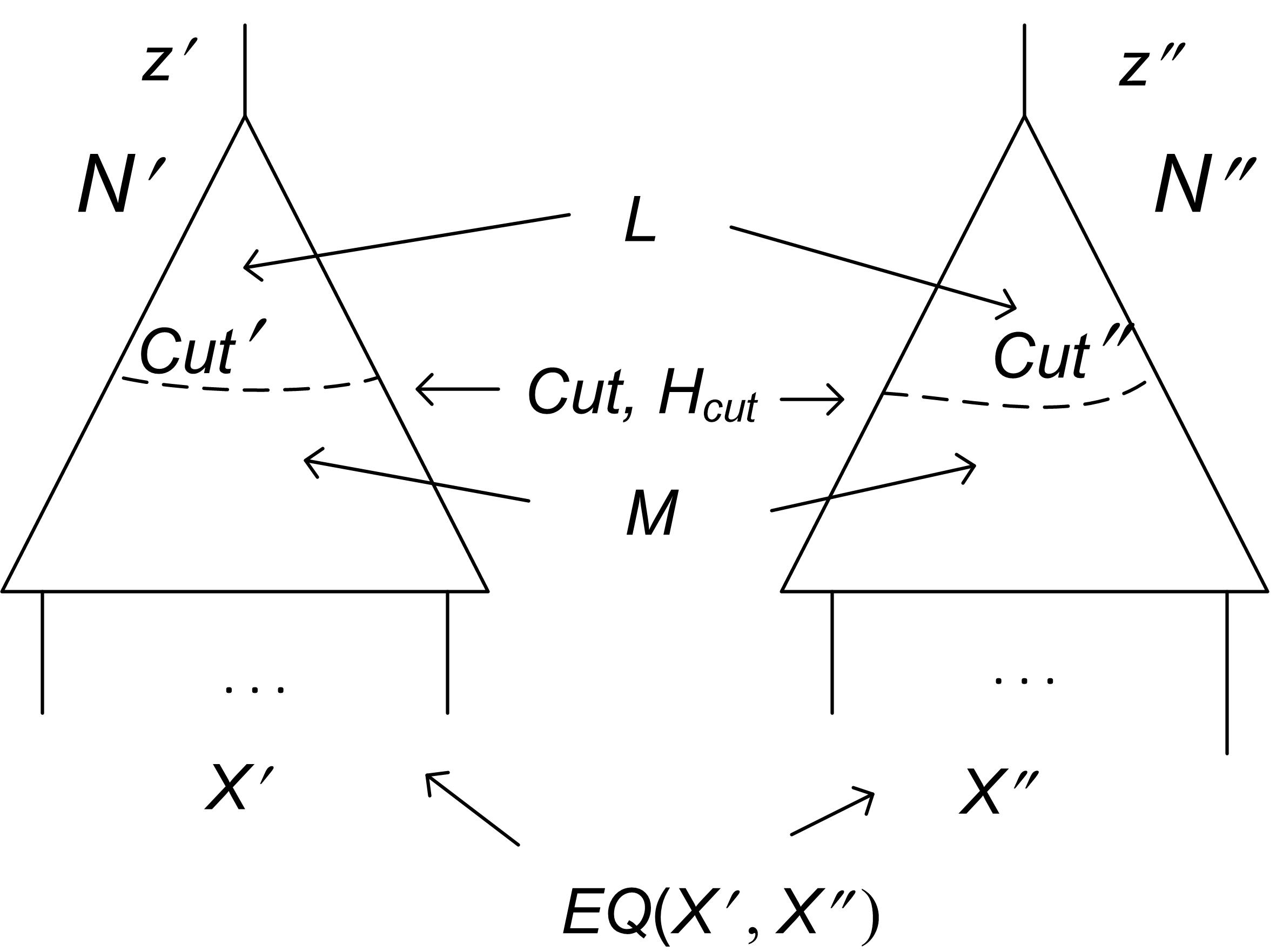
Figure 7: Replacing/Separa-ting boundary formula $\mathit{H}_{\mathit{cut}}$

In this subsection, we discuss the difference between boundary formulas and interpolants in the context of EC. Let formulas $F_{M}$ and $F_{L}$ specify the gates located below and above a cut as shown in Fig. 7. Then checking the equivalence of $N^{\prime}$ and $N^{\prime\prime}$ comes down to testing the satisfiability of formula $S$ equal to $\mathit{EQ}(X^{\prime},X^{\prime\prime})\wedge F_{M}\wedge F_{L}\wedge(z^{\prime}\not\equiv z^{\prime\prime})$.

Below, we contrast two types of relaxation of formula $S$ called replacing and separating relaxation. The former corresponds to interpolation while the latter is the relaxation we studied in the previous sections. A replacing relaxation of $S$ is to drop the clauses of $\mathit{EQ}\wedge F_{M}$. That is $\mathit{S}^{\mathit{rlx}}$ = $F_{L}\wedge(z^{\prime}\not\equiv z^{\prime\prime})$. Let $\mathit{H}_{\mathit{cut}}^{\mathit{r}}$ be a boundary formula computed for replacing relaxation. (Superscript $r$ stands for “replacing”.) That is $\exists{W}[\mathit{EQ}\wedge F_{M}\wedge F_{L}\wedge(z^{\prime}\not\equiv z^{\prime\prime})]$ $\equiv\mbox{$\mathit{H}_{\mathit{cut}}^{\mathit{r}}$}\wedge\mbox{$\exists{W}[F_{L}\wedge(z^{\prime}\not\equiv z^{\prime\prime})]$}$ where $W$ consists of all the variables of $S$ but cut variables. Note that $\mathit{H}_{\mathit{cut}}^{\mathit{r}}$ replaces all clauses depending on variables corresponding to gates below the cut, hence the name replacing relaxation. Let $A$ denote formula $\mathit{EQ}\wedge F_{M}$ and $B$ denote formula $F_{L}\wedge(z^{\prime}\not\equiv z^{\prime\prime})$. From Proposition 8 it follows that if $A\rightarrow\mbox{$\mathit{H}_{\mathit{cut}}^{\mathit{r}}$}$ and $A\wedge B\equiv 0$ then $\mathit{H}_{\mathit{cut}}^{\mathit{r}}$ is an interpolant of implication $A\rightarrow\overline{B}$. So an interpolant can be viewed as a boundary formula for replacing relaxation.

A separating relaxation of $S$ is to drop the clauses of $\mathit{EQ}$. As we mentioned above, this kind of relaxation has been the focus of the previous sections. Let $\mathit{H}_{\mathit{cut}}^{\mathit{s}}$ denote a boundary formula for separating relaxation. (Superscript $s$ stands for “separating”.) Formula $\mathit{H}_{\mathit{cut}}^{\mathit{s}}$ satisfies $\exists{W}[\mathit{EQ}\wedge F_{M}\wedge F_{L}\wedge(z^{\prime}\not\equiv z^{\prime\prime})]$ $\equiv\mbox{$\mathit{H}_{\mathit{cut}}^{\mathit{s}}$}\wedge$ $\exists{W}[F_{M}\wedge F_{L}\wedge(z^{\prime}\not\equiv z^{\prime\prime})]$. Note that adding formula $\mathit{H}_{\mathit{cut}}^{\mathit{s}}$ separates input variables $X^{\prime}$ and $X^{\prime\prime}$ of $N^{\prime}$ and $N^{\prime\prime}$ by making formula $\mathit{EQ(X^{\prime},X^{\prime\prime})}$ redundant, hence the name separating relaxation. We will refer to $\mathit{H}_{\mathit{cut}}^{\mathit{r}}$ and $\mathit{H}_{\mathit{cut}}^{\mathit{s}}$ as replacing and separating boundary formulas respectively.

Let us assume for the sake of simplicity that a replacing boundary formula $\mathit{H}_{\mathit{cut}}^{\mathit{r}}$ is an interpolant i.e. it is implied by $\mathit{EQ}\wedge F_{M}$. We will also assume that a separating boundary formula $\mathit{H}_{\mathit{cut}}^{\mathit{s}}$ satisfies the condition of Proposition 2 and hence is implied by $\mathit{EQ}\wedge F_{M}$ as well. An obvious difference between $\mathit{H}_{\mathit{cut}}^{\mathit{r}}$ and $\mathit{H}_{\mathit{cut}}^{\mathit{s}}$ is as follows. Adding $\mathit{H}_{\mathit{cut}}^{\mathit{s}}$ to formula $\exists{W}[\mathit{EQ}\wedge F_{M}\wedge F_{L}\wedge(z^{\prime}\not\equiv z^{\prime\prime})]$ makes redundant only a subset of clauses that is made redundant after adding $\mathit{H}_{\mathit{cut}}^{\mathit{r}}$. The fact that adding $\mathit{H}_{\mathit{cut}}^{\mathit{r}}$ has to make redundant both clauses of $EQ$ and $F_{M}$ creates the following problem with using interpolants for equivalence checking. On the one hand, since $\mathit{H}_{\mathit{cut}}^{\mathit{r}}$ is implied by $\mathit{EQ}\wedge F_{M}$, the former can be obtained by resolving clauses of the latter i.e. without looking at the part of $N^{\prime}$ and $N^{\prime\prime}$ above the cut. On the other hand, proving that $\mathit{H}_{\mathit{cut}}^{\mathit{r}}$ is indeed an interpolant, in general, requires checking that $\mbox{$\mathit{H}_{\mathit{cut}}^{\mathit{r}}$}\wedge F_{L}\wedge(z^{\prime}\not\equiv z^{\prime\prime})\equiv 0$ and hence needs the knowledge of the part of $N^{\prime}$ and $N^{\prime\prime}$ above the cut.

Informally, the problem above means that one cannot build a small interpolant $\mathit{H}_{\mathit{cut}}^{\mathit{r}}$ using only clauses of $\mathit{EQ}\wedge F_{M}$. By contrast, one can construct a small separating boundary formula without any knowledge of formula $F_{L}$. Let us consider the following simple example. Suppose that the cut of Fig. 7 is an equivalence cut. That is for for every cut point of $N^{\prime}$ there is a functionally equivalent cut point of $N^{\prime\prime}$ and vice versa. From Corollary 2 it follows that formula $\mathit{EQ}(\mathit{Cut^{\prime}},\mathit{Cut^{\prime\prime}})$ is a separating boundary formula. (Here $\mathit{Cut^{\prime}}$ and $\mathit{Cut^{\prime\prime}}$ specify the cut points of $N^{\prime}$ and ^′′ respectively.) This fact can be established from formula $\mathit{EQ}\wedge F_{M}$ alone. However, whether $\mathit{EQ}(\mathit{Cut^{\prime}},\mathit{Cut^{\prime\prime}})$ is an interpolant of implication $A\rightarrow\overline{B}$ (where $A=\mathit{EQ}(X^{\prime},X^{\prime\prime})\wedge F_{M}$ and $B=F_{L}\wedge(z^{\prime}\not\equiv z^{\prime\prime})$) totally depends on formula $F_{L}$ i.e. on the part of $N^{\prime}$ and $N^{\prime\prime}$ above the cut.

10 Conclusions

We introduced a new framework for Equivalence Checking (EC) based on Lo-gic Relaxation (LoR). The appeal of applying LoR to EC is twofold. First, EC by LoR provides a powerful method for generating proofs of equivalence by induction. Second, LoR gives a framework for proving inequivalence without generating a counterexample. The idea of LoR is quite general and can be applied beyond EC. LoR is enabled by a technique called partial quantifier elimination and the performance of the former strongly depends on that of the latter. So building efficient algorithms of partial quantifier elimination is of great importance.

Appendix

Appendix 0.A Proofs Of Propositions

Proposition 1

Let $H(z^{\prime},z^{\prime\prime})$ be a formula such that $\mbox{$\exists{W}[\mathit{EQ}\wedge\mbox{$\mathit{G}^{\mathit{rlx}}$}]$}\equiv$ $H\wedge\mbox{$\exists{W}[\mbox{$\mathit{G}^{\mathit{rlx}}$}]$}$ where $W=X^{\prime}\cup X^{\prime\prime}\cup Y^{\prime}\cup Y^{\prime\prime}$. Then formula $G\wedge(z^{\prime}\not\equiv z^{\prime\prime})$ is equisatisfiable with $H\wedge\mbox{$\mathit{G}^{\mathit{rlx}}$}\wedge(z^{\prime}\not\equiv z^{\prime\prime})$.

Proof

A proof of this proposition follows from Propositions 2 and 3 below. Proposition 2 entails that $H(z^{\prime},z^{\prime\prime})$ is a boundary formula. From Proposition 3 it follows that $G\wedge(z^{\prime}\not\equiv z^{\prime\prime})$ is equisatisfiable with $H\wedge\mbox{$\mathit{G}^{\mathit{rlx}}$}\wedge(z^{\prime}\not\equiv z^{\prime\prime})$.

Proposition 2

Let $\mathit{H}_{\mathit{cut}}$ be a formula depending only on variables of a cut. Let $\mathit{H}_{\mathit{cut}}$ satisfy $\mbox{$\exists{W}[\mathit{EQ}\wedge F_{M}]$}\equiv\mbox{$\mathit{H}_{\mathit{cut}}$}\wedge\mbox{$\exists{W}[F_{M}]$}$. Here $W$ is the set of variables of $F_{M}$ minus those of the cut. Then $\mathit{H}_{\mathit{cut}}$ is a boundary formula.

Proof

$\mbox{$\exists{W}[\mathit{EQ}\wedge F_{M}]$}\equiv\mbox{$\mathit{H}_{\mathit{cut}}$}\wedge\mbox{$\exists{W}[F_{M}]$}$ entails $\mathit{EQ}\wedge F_{M}\rightarrow\mbox{$\mathit{H}_{\mathit{cut}}$}$. Let $L$ be the subcircuit consisting of the gates of $N^{\prime}$ and $N^{\prime\prime}$ located above the cut. Let $F_{L}$ be a formula specifying $L$. Since $G=\mathit{EQ}\wedge F_{M}\wedge F_{L}$, then $G\rightarrow\mbox{$\mathit{H}_{\mathit{cut}}$}$ and so condition a) of Definition 1 is met. Let us prove that condition b) is met as well. Let $q$ be a cut assignment that can be extended to satisfy $\mathit{G}^{\mathit{rlx}}$ but not $G$. This means that $q$ cannot be extended to an assignment $p$ satisfying $\mathit{EQ}\wedge F_{M}$ either. (Otherwise, one could easily extend $p$ to an assignment satisfying $\mathit{EQ}\wedge F_{M}\wedge F_{L}$ and hence $G$ by using the values of an execution trace computed for circuit $L$. This trace describes computation of output values of $L$ when its input variables i.e. the cut variables are assigned as in $q$.) So $\exists{W}[\mathit{EQ}\wedge F_{M}]$=0 under assignment $q$. This means that $\mbox{$\mathit{H}_{\mathit{cut}}$}\wedge\mbox{$\exists{W}[F_{M}]$}=0$ under assignment $q$. Taking into account that $q$ can be extended to an assignment satisfying $\mathit{G}^{\mathit{rlx}}$ and hence $F_{M}$, one has to conclude that $\mbox{$\mathit{H}_{\mathit{cut}}$}({\mbox{\boldmath$q$}})=0$.

Proposition 3

Let $\mathit{H}_{\mathit{cut}}$ be a boundary formula with respect to a cut. Then $G\wedge(z^{\prime}\not\equiv z^{\prime\prime})$ is equisatisfiable with $\mbox{$\mathit{H}_{\mathit{cut}}$}\wedge\mbox{$\mathit{G}^{\mathit{rlx}}$}\wedge(z^{\prime}\not\equiv z^{\prime\prime})$.

Proof

Let us show that the satisfiability of the left formula i.e. $G\wedge(z^{\prime}\not\equiv z^{\prime\prime})$ implies that of the right formula i.e. $\mbox{$\mathit{H}_{\mathit{cut}}$}\wedge\mbox{$\mathit{G}^{\mathit{rlx}}$}\wedge(z^{\prime}\not\equiv z^{\prime\prime})$ and vice versa.

Left sat. $\rightarrow$ Right sat. Let $p$ be an assignment satisfying $G\wedge(z^{\prime}\not\equiv z^{\prime\prime})$. From Definition 1 it follows that $G$ implies $\mathit{H}_{\mathit{cut}}$ and so $\mathit{H}_{\mathit{cut}}$ is satisfied by $p$. Since $\mathit{G}^{\mathit{rlx}}$ is a subformula of $G$, assignment $p$ satisfies $\mathit{G}^{\mathit{rlx}}$ as well. Hence $p$ satisfies $\mbox{$\mathit{H}_{\mathit{cut}}$}\wedge\mbox{$\mathit{G}^{\mathit{rlx}}$}\wedge(z^{\prime}\not\equiv z^{\prime\prime})$.

Right sat. $\rightarrow$ Left sat. Let $p$ be an assignment satisfying $\mbox{$\mathit{H}_{\mathit{cut}}$}\wedge\mbox{$\mathit{G}^{\mathit{rlx}}$}\wedge(z^{\prime}\not\equiv z^{\prime\prime})$. Let $q$ be the subset of $p$ consisting of the assignments to the cut variables. Since $\mathit{H}_{\mathit{cut}}$($q$)=1, Definition 1 entails that $q$ can be extended to an assignment $p^{*}$ satisfying formula $G$. Since the variables assigned in $q$ form a cut of circuits $N^{\prime}$ and $N^{\prime\prime}$, the consistent assignments to the variables of $N^{\prime}$ and $N^{\prime\prime}$ located above the cut are identical in $p$ and $p^{*}$. This means that $p^{*}$ satisfies $(z^{\prime}\not\equiv z^{\prime\prime})$ and hence formula $G\wedge(z^{\prime}\not\equiv z^{\prime\prime})$.

Proposition 4

Let $\mathit{Cut^{\prime}},\mathit{Cut}^{\prime\prime}$ specify the outputs of circuits $M^{\prime}$ and $M^{\prime\prime}$ of Fig. 4 respectively. Assume that for every variable $v^{\prime}$ of $\mathit{Cut^{\prime}}$ there is a set $S(v^{\prime})=\mbox{$\{v^{\prime\prime}_{i_{1}},\dots,v^{\prime\prime}_{i_{k}}\}$}$ of variables of $\mathit{Cut^{\prime\prime}}$ that have the following property. Knowing the values of variables of $S(v^{\prime})$ produced in $N^{\prime\prime}$ under input $x$ one can determine the value of $v^{\prime}$ of $N^{\prime}$ under the same input $x$. We assume here that $S(v^{\prime})$ has this property for every possible input $x$. Let $\mathit{Max}(S(v^{\prime}))$ be the size of the largest $S(v^{\prime})$ over variables of $\mathit{Cut^{\prime}}$. Then there is a boundary formula $\mathit{H}_{\mathit{cut}}$ where every clause has at most $\mathit{Max}(S(v^{\prime}))+1$ literals.

Proof

Let $q$ be an assignment to the cut variables that can be extended to satisfy formula $\mathit{G}^{\mathit{rlx}}$ but not formula $G$. To prove the proposition at hand, one needs to show that there is a clause $C$ consisting of cut variables such that

• $C$ is implied by formula $G$

• $C({\mbox{\boldmath$q$}})=0$

• $C$ consists of at most $\mathit{Max}(S(v^{\prime}))$ literals

(Using clauses satisfying the three conditions above one can build a required boundary formula $\mathit{H}_{\mathit{cut}}$.)

Let $p$ be an assignment satisfying formula $\mathit{G}^{\mathit{rlx}}$ that is obtained by extending $q$. Let $x^{\prime}$ and $x^{\prime\prime}$ be the assignments of $p$ to variables of $X^{\prime}$ and $X^{\prime\prime}$ respectively. Note that ${\mbox{\boldmath$x^{\prime}$}}\neq{\mbox{\boldmath$x^{\prime\prime}$}}$ (otherwise $p$ would satisfy formula $G$ as well). Cut assignment $q$ can be represented as ($q^{\prime}$,$q^{\prime\prime}$) where $q^{\prime}$ and $q^{\prime\prime}$ are assignments of $q$ to $\mathit{Cut^{\prime}}$ and $\mathit{Cut^{\prime\prime}}$ respectively. Assignment $q^{\prime}$ (respectively $q^{\prime\prime}$) is produced by circuit $M^{\prime}$ (respectively $M^{\prime\prime}$) under input $x^{\prime}$ (respectively $x^{\prime\prime}$).

Let $v^{\prime}$ be a variable of $\mathit{Cut}^{\prime}$. The value of $v^{\prime}$ is uniquely specified by assignment $q^{\prime\prime}$ to $S(v^{\prime})$. So the value of every variable of $\mathit{Cut}^{\prime}$ is specified by assignment $q^{\prime\prime}$ to $\mathit{Cut}^{\prime\prime}$. Denote by $s^{\prime}$ the assignment to $\mathit{Cut^{\prime}}$ specified by $q^{\prime\prime}$. Let us show that ${\mbox{\boldmath$s^{\prime}$}}\neq{\mbox{\boldmath$q^{\prime}$}}$. Assume the contrary i.e. $s^{\prime}$ = $q^{\prime}$ and show that then one can extend $q$ to an assignment $p^{*}$ satisfying formula $G$ and so we have a contradiction. Assignment $p^{*}$ is constructed as follows. The variables below the cut are assigned in $p^{*}$ as in the execution trace obtained by applying $x^{\prime\prime}$ to $M^{\prime}$ and $M^{\prime\prime}$. Note that by assumption, applying input $x^{\prime\prime}$ to $M^{\prime}$ will produce cut assignment $s^{\prime}$ equal to $q^{\prime}$. The variables above the cut are assigned in $p^{*}$ as in $p$. Since $p$ satisfies $\mathit{G}^{\mathit{rlx}}$ and $X^{\prime}$ and $X^{\prime\prime}$ are assigned the same input $x^{\prime\prime}$ in $p^{*}$, the latter satisfies $G$. Besides, the cut assignment specified by $p^{*}$ is $q$ i.e. the same as the one specified by $p$.

Since ${\mbox{\boldmath$q^{\prime}$}}\neq{\mbox{\boldmath$s^{\prime}$}}$, there is a variable $v^{\prime}$ of $\mathit{Cut^{\prime}}$ that is assigned in $q^{\prime}$ inconsistently with the assignment of $q^{\prime\prime}$ to the variables of $S(v^{\prime})$. Let $C^{\prime\prime}$ be the clause of variables of $S(v^{\prime})$ falsified by $q^{\prime\prime}$. Let $l(v^{\prime})$ be the literal of $v^{\prime}$ falsified by $q^{\prime}$. Then clause $l(v^{\prime})\vee C^{\prime\prime}$ is falsified by $q$. The fact that assignment $q^{\prime}$ to $S(v^{\prime})$ determines the value of $v^{\prime}$ means that clause $l(v^{\prime})\vee C^{\prime\prime}$ is implied by formula $F_{M^{\prime}}\wedge F_{M^{\prime\prime}}$. Hence $l(v^{\prime})\vee C^{\prime\prime}$ is implied by $G$. Finally, the number of literals in $l(v^{\prime})\vee C^{\prime\prime}$ is $|S(v^{\prime})|+1$. So clause $l(v^{\prime})\vee C^{\prime\prime}$ satisfies the three conditions above.

Proposition 5

Let $W_{i}$ where $i>0$ be the set of variables of $F_{M_{i}}$ minus those of $\mathit{Cut}_{i}$. Let $H_{i-1}$ where $i>1$ be a boundary formula such that $\mbox{$\exists{W_{i-1}}[H_{0}\wedge F_{M_{i-1}}]$}\equiv H_{i-1}\wedge\exists{W_{i-1}}[F_{M_{i-1}}]$. Let $\mbox{$\exists{W_{i}}[H_{i-1}\wedge F_{M_{i}}]$}\equiv H_{i}\wedge\mbox{$\exists{W_{i}}[F_{M_{i}}]$}$ hold. Then $\exists{W_{i}}[H_{0}\wedge F_{M_{i}}]$ $\equiv$ $H_{i}\wedge\mbox{$\exists{W_{i}}[F_{M_{i}}]$}$ holds. (So $H_{i}$ is a boundary formula due to Proposition 2.)

Proof

Let $\phi$ denote formula $\exists{W_{i}}[H_{0}\wedge F_{M_{i}}]$. Let $F_{i-1,i}$ be the set of clauses equal to $F_{M_{i}}\setminus F_{M_{i-1}}$. Formula $\phi$ can be represented as $\exists{W_{i-1}}\exists{W_{i-i,i}}[H_{0}\wedge F_{M_{i-1}}\wedge F_{i-1,i}]$ where $W_{i-1,i}=W_{i}\setminus W_{i-1}$. Taking into account that formula $F_{i-1,i}$ does not depend on variables of $W_{i-1}$, one can rewrite formula $\phi$ as $\exists{W_{i-1,i}}[F_{i-1,i}\wedge\mbox{$\exists{W_{i-1}}[H_{0}\wedge F_{M_{i-1}}]$}]$. Using the assumption imposed on $H_{i-1}$ by the proposition at hand, one can transform formula $\phi$ into $\exists{W_{i-1,i}}[F_{i-1,i}\wedge H_{i-1}\wedge\mbox{$\exists{W_{i-1}}[F_{M_{i-1}}]$}]$. After putting $F_{i-1,i}$ and $H_{i-1}$ back under the scope of quantifiers, $\phi$ becomes equal to $\exists{W_{i-1,i}}[\mbox{$\exists{W_{i-1}}[H_{i-1}\wedge F_{M_{i-1}}\wedge F_{i-1,i}]$}]$ and hence to $\exists{W_{i}}[H_{i-1}\wedge F_{M_{i}}]$. Since $\mbox{$\exists{W_{i}}[H_{i-1}\wedge F_{M_{i}}]$}\equiv H_{i}\wedge\mbox{$\exists{W_{i}}[F_{M_{i}}]$}$ holds we get that the original formula $\phi$ equal to $\exists{W_{i}}[H_{0}\wedge F_{M_{i}}]$ is logically equivalent to $H_{i}\wedge\mbox{$\exists{W_{i}}[F_{M_{i}}]$}$.

Proposition 6

Let $S(X,Z)$, $\mbox{$\mathit{S}^{\mathit{rlx}}$}(X,Z)$, $E(X,Z)$ and $H(Z)$ be Boolean formulas where $X,Z$ are non-overlapping sets of variables. Let $S=E\wedge\mbox{$\mathit{S}^{\mathit{rlx}}$}$ and $\mbox{$\exists{X}[E\wedge\mbox{$\mathit{S}^{\mathit{rlx}}$}]$}\equiv H\wedge\mbox{$\exists{X}[\mbox{$\mathit{S}^{\mathit{rlx}}$}]$}$ hold. Then $S$ is equisatisfiable with $H\wedge\mbox{$\mathit{S}^{\mathit{rlx}}$}$.

Proof

By assumptions of the proposition, $\mbox{$\exists{X}[S]$}\equiv\mbox{$\exists{X}[H\wedge\mbox{$\mathit{S}^{\mathit{rlx}}$}]$}$. So if formula $S$ is satisfiable, there is an assignment $z$ to the variables of $Z$ for which $\exists{X}[S]$ evaluates to 1. Since formula $\exists{X}[H\wedge\mbox{$\mathit{S}^{\mathit{rlx}}$}]$ also evaluates to 1 for $z$, formula $H\wedge\mbox{$\mathit{S}^{\mathit{rlx}}$}$ is satisfiable too. Similarly, one can show that the satisfiability of $\exists{X}[H\wedge\mbox{$\mathit{S}^{\mathit{rlx}}$}]$ means that that $S$ is satisfiable too.

Proposition 7

Let formula $S(X,Z)$ be represented as $E(X,Z)\wedge\mbox{$\mathit{S}^{\mathit{rlx}}$}(X,Z)$ where $X,Z$ are non-overlapping sets of Boolean variables. Let $\mbox{$\exists{X}[E\wedge\mbox{$\mathit{S}^{\mathit{rlx}}$}]$}\equiv H\wedge\mbox{$\exists{X}[\mbox{$\mathit{S}^{\mathit{rlx}}$}]$}$ hold for a formula $H(Z)$. Then $H$ is a boundary formula in terms of $Z$ for relaxation $\mathit{S}^{\mathit{rlx}}$ (see Definition 1). That is

1. $S\rightarrow H$ and

2. for every assignment $z$ to $Z$ that can be extended to satisfy $\mathit{S}^{\mathit{rlx}}$ but not $S$, the value of $H({\mbox{\boldmath$z$}})$ is 0.

Proof

$\mbox{$\exists{X}[E\wedge\mbox{$\mathit{S}^{\mathit{rlx}}$}]$}\equiv H\wedge\mbox{$\exists{X}[\mbox{$\mathit{S}^{\mathit{rlx}}$}]$}$ entails $E\wedge\mbox{$\mathit{S}^{\mathit{rlx}}$}\rightarrow H$. So condition a) is met. Let us show that condition b) holds as well. Let $z$ be an assignment to $Z$ that can be extended to satisfy $\mathit{S}^{\mathit{rlx}}$ but not $S$. This means that $\exists{X}[E\wedge\mbox{$\mathit{S}^{\mathit{rlx}}$}]$ and $\exists{X}[\mbox{$\mathit{S}^{\mathit{rlx}}$}]$ evaluate to 0 and 1 respectively under assignment $z$. Hence $H({\mbox{\boldmath$z$}})$ has to be equal to 0 to preserve $\mbox{$\exists{X}[E\wedge\mbox{$\mathit{S}^{\mathit{rlx}}$}]$}\equiv H\wedge\mbox{$\exists{X}[\mbox{$\mathit{S}^{\mathit{rlx}}$}]$}$.

Proposition 8

Let $A(X,Y)$ and $B(Y,Z)$ be formulas where $X,Y,Z$ are non-overlapping sets of variables. Let $A\wedge B\equiv 0$. Formula $H(Y)$ is an interpolant of implication $A\rightarrow\overline{B}$ iff $A\rightarrow H$ and $\mbox{$\exists{W}[A\wedge B]$}\equiv H\wedge\mbox{$\exists{W}[B]$}$ where $W=X\cup Z$.

Proof

If part. Suppose that $A\rightarrow H$ holds and $\mbox{$\exists{W}[A\wedge B]$}\equiv H\wedge\mbox{$\exists{W}[B]$}$. Since $A\rightarrow\overline{B}$ holds, then $A\wedge B\equiv 0$ and so $H\wedge B\equiv 0$. Hence $H\rightarrow\overline{B}$ and $H$ is an interpolant of implication $A\rightarrow\overline{B}$.

Only if part. Suppose that $H$ is an interpolant and so $A\rightarrow H$ and $H\rightarrow\overline{B}$ hold. Assume that $\mbox{$\exists{W}[A\wedge B]$}\not\equiv H\wedge\mbox{$\exists{W}[B]$}$. Since $H\rightarrow\overline{B}$ and hence $H\wedge B\equiv 0$, this means that $A\wedge B\not\equiv 0$. So we have a contradiction.

Proposition 9

Let $A(X,Y)\wedge B(Y,Z)\not\equiv 0$ where $X,Y,Z$ are non-overlapping sets of variables. Let $H(Y)$ be a formula such that $\mbox{$\exists{W}[A\wedge B]$}\equiv H\wedge\mbox{$\exists{W}[B]$}$ where $W=X\cup Z$. Let $y$ and $z$ be assignments to $Y$ and $Z$ respectively such that ($y$,$z$) satisfies $H\wedge B$. Then ($y$,$z$) can be extended to an assignment satisfying $A\wedge B$.

Proof

The fact that $\mbox{$\exists{W}[A\wedge B]$}\equiv H\wedge\mbox{$\exists{W}[B]$}$ holds and $H\wedge B$ is satisfied by ($y$,$z$) means that $y$ can be extended to an assignment ($x^{*}$,$y$,$z^{*}$) satisfying $A\wedge B$. Then assignment ($x^{*}$,$y$,$z$) satisfies $A\wedge B$ as well. Indeed, ($x^{*}$,$y$) satisfies $A$ and ($y$,$z$) does $B$.

Appendix 0.B Algorithm For Partial Quantifier Elimination

In this section, we discuss Partial Quantifier Elimination (PQE) in more detail. In Subsection 0.B.1, we give a high-level description of a PQE-solver. This PQE-solver is based on the machinery of Dependency sequents (D-sequents) that we recall in Subsection 0.B.2.

0.B.1 A PQE solver

In this subsection, we describe our algorithm for PQE introduced in [9] in 2014. We will use the same name for this algorithm as in Section 7, i.e. PQE-14. Let $A(V,W),B(V,W)$ be Boolean formulas where $V$,$W$ are non-overlapping sets of variables. As we mentioned in Subsection 3.1, the PQE problem is to find formula $A^{*}(V)$ such that $\mbox{$\exists{W}[A\wedge B]$}\equiv A^{*}\wedge\mbox{$\exists{W}[B]$}$. We will refer to a clause containing a variable of $W$ as a $W$-clause. PQE-14 is based on the three ideas below.

First, finding formula $A^{*}$ comes down to generation of clauses depending only on variables of $V$ that make the $W$-clauses of $A$ redundant in $A^{*}\wedge\mbox{$\exists{W}[A\wedge B]$}$. Second, the clauses of $A^{*}$ can be derived by resolving clauses of $A\wedge B$. The intermediate resolvents that are $W$-clauses need to be proved redundant along with the original $W$-clauses of $A$. However, since formula $B$ remains quantified, there is no need to prove redundancy of $W$-clauses of $B$ or $W$-clauses obtained by resolving only clauses of $B$.

Third, since proving redundancy of a clause is a hard problem it makes sense to partition this problem into simpler subproblems. To this end, PQE-14 employs branching. After proving redundancy of required clauses in subspaces, the results of branches are merged. The advantage of branching is that for every $W$-clause $C$ one can always reach a subspace where $C$ can be trivially proved redundant. Namely, $C$ is trivially redundant in the current subspace if a) $C$ is satisfied in the current branch; b) $C$ is implied by some other clause; c) there is an unassigned variable $y$ of $C$ where $y\in W$, such that $C$ cannot be resolved on $y$ with other clauses that are not satisfied or proved redundant yet.

0.B.2 Dependency sequents

PQE-14 branches on variables of $V\cup W$ until the $W$-clauses that are descendants of $W$-clauses of $A$ are proved redundant in the current subspace. To keep track of conditions under which a $W$-clause becomes redundant in a subspace, PQE-14 uses the machinery of Dependency sequents (D-sequents) developed in [7, 8]. A D-sequent is a record of the form $(\mbox{$\exists{W}[A\wedge B]$},{\mbox{\boldmath$q$}})~{}\rightarrow\mbox{$\{C\}$}$. It states that clause $C$ is redundant in formula $\exists{W}[A\wedge B]$ in subspace $q$. Here $q$ is an assignment to variables of $V\wedge W$ and $A$ is the current formula that consists of the initial clauses of $A$ and the resolvent clauses. When a $W$-clause $C$ is proved redundant in a subspace, this fact is recorded as a D-sequent. If ${\mbox{\boldmath$q$}}=\emptyset$, the D-sequent is called unconditional. Derivation of such a D-sequent means that clause $C$ is redundant in the current formula $\exists{W}[A\wedge B]$ in the entire space.

The objective of PQE-14 is to derive unconditional D-sequents for all $W$-clauses of $A$ and their descendants that are $W$-clauses. A new D-sequent can be obtained from two parent D-sequents by a resolution-like operation on a variable $y$. This operation is called join. When PQE-14 merges the results of branching on variable $y$ it joins D-sequents obtained in branches $y=0$ and $y=1$ at variable $y$. So the resulting D-sequents do not depend on $y$. If formula $A\wedge B$ is unsatisfiable in both branches, a new clause $C$ is added to formula $A$. Clause $C$ is obtained by resolving a clause falsified in subspace $y=0$ with a clause falsified in subspace $y=1$ on $y$. Adding $C$ makes all $W$-clauses redundant in the current subspace. By the time PQE-14 backtracks to the root of the search tree, it has derived unconditional D-sequents for all $W$-clauses of the current formula $A$.

Algorithms based on D-sequents (including PQE solving) is work in progress. So they still lack some important techniques like D-sequent re-using. In the current algorithms based on D-sequents, the parent D-sequents are discarded as soon as they produce a new D-sequent by the join operation. Although D-sequent re-using promises to be as powerful as re-using learned clauses in SAT-solving, it requires more sophisticated bookkeeping and so is not implemented yet [9].

Appendix 0.C Generation Of Cuts That Do Not Overlap

An important part of $\mathit{EC\!\_LoR}$ described in Section 5 is to build non-overlapping cuts. These cuts are used to generate a sequence of boundary formulas converging to an output boundary formula. As we mentioned there, the presence of non-local connections makes it hard to find cuts that do not overlap. In this section, we consider this issue in more detail. First, we give the necessary definitions and describe the problem. Then we explain how one can get rid of non-local connections by buffer insertion.

Let $M$ be a multi-output circuit. The length of a path from an output of a gate to an input of another gate is measured by the number of gates on this path.The topological level of a gate $g$ is the longest path from an input of $M$ to $g$. We treat the inputs of $M$ as special gates that are not fed by other gates. We will denote the topological level of gate $g$ as $\mathit{TopLvl}(g)$. It can be computed recursively as follows. If $g$ is an input, then $\mathit{TopLvl}(g)$ = 0. Otherwise, $\mathit{TopLvl}(g)$ is equal to the maximum topological level among the gates feeding $g$ plus 1.

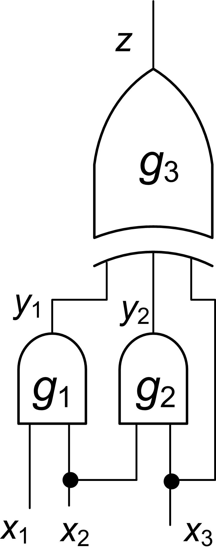
Figure 8: A circuit

We will call gates $g_{i}$ and $g_{j}$ topologically independent if there is no path from an input to an output of $M$ going through both these gates. For instance, gates $g_{1}$ and $g_{2}$ in Fig. 8 are topologically independent. We will call a set $S$ of gates a cut, if every path from an input to an output of $M$ goes through a gate of $S$. A cut $S$ is minimal, if for every gate $g\in S$, set $S\setminus\mbox{$\{g\}$}$ is not a cut. $\mathit{EC\!\_LoR}$ employs only minimal cuts. In this section, we use the notion of a gate and the variable specifying its output interchangeably. For example, the topological level of a variable $v$ specifying the output of gate $g$ (denoted as $\mathit{TopLvl}(v)$) is equal to $\mathit{TopLvl}(g)$.

If gate $g_{i}$ of $M$ feeds gate $g_{j}$ and $\mbox{$\mathit{TopLvl}(g_{j})$}>\mbox{$\mathit{TopLvl}(g_{i})$}+1$, then $g_{i}$ and $g_{j}$ are said to have a non-local connection. Non-local connections make topologically dependent gates appear on the same cut. Consider the circuit of Fig 8. The input gate $x_{3}$ feeds gates $g_{2}$ and $g_{3}$. Since $\mathit{TopLvl}(x_{3})$=0 and $\mathit{TopLvl}(g_{3})$=2, the connection between $x_{3}$ and $g_{3}$ is non-local. This leads to appearance of cut $\{y_{1},y_{2},x_{3}\}$ where variables $y_{2}$ and $x_{3}$ are topologically dependent. If gate $g_{i}$ feeds gate $g_{j}$ and this connection is non-local, gate $g_{i}$ appears in every cut that separates $g_{i}$ and $g_{j}$ and does not include $g_{j}$. So the presence of a large number of non-local connections leads to the heavy overlapping of cuts.

There are a few techniques for dealing with non-local connections of $N^{\prime}$ and $N^{\prime\prime}$ in the context of EC by LoR. The simplest one is to insert buffers. A buffer is a single-input and single-output gate that copies its input to the output. Let $g_{i}$ and $g_{j}$ be gates of $N^{\prime}$ such that a) $g_{i}$ feeds $g_{j}$ and b) $\mbox{$\mathit{TopLvl}(g_{j})$}>\mbox{$\mathit{TopLvl}(g_{i})$}+1$. By inserting $\mbox{$\mathit{TopLvl}(g_{j})$}-\mbox{$\mathit{TopLvl}(g_{i})$}-1$ buffers between $g_{i}$ to $g_{j}$, this non-local connection is replaced with $\mbox{$\mathit{TopLvl}(g_{j})$}-\mbox{$\mathit{TopLvl}(g_{i})$}$ local connections.

Appendix 0.D Version of $\mathit{EC\!\_LoR}$ Used In Experiments

In the experiments of Subsection 7.2, we used a version of $\mathit{EC\!\_LoR}$ that was modified in comparison to the description given in Fig. 5. We will refer to this version as $\mathit{EC\!\_LoR}^{*}$. In this section, we describe $\mathit{EC\!\_LoR}^{*}$ in more detail.

Boundary formula $H_{i}$ was computed in $\mathit{EC\!\_LoR}^{*}$ as follows. If there was a variable specifying the output of a cut gate $g^{\prime}$ that was not present in a clause of $H_{i}$, $\mathit{EC\!\_LoR}^{*}$ called the procedure below. That procedure generated short clauses relating the output variable of $g^{\prime}$ and those of its “relatives” from $N^{\prime\prime}$. This way, $\mathit{EC\!\_LoR}^{*}$ avoided running a cut termination check before every variable of $i$-th cut was present in a clause of $H_{i}$.

Clauses of $H_{i}$ constraining variable of $g^{\prime}$ were generated as follows. First, $\mathit{EC\!\_LoR}^{*}$ identified the relatives $g^{\prime\prime}_{1},\dots,g^{\prime\prime}_{m}$ of gate $g^{\prime}$ in $N^{\prime\prime}$. A gate $g^{\prime\prime}_{j}$ was considered a relative of $g^{\prime}$ if there was a clause of formula $H_{i-1}$ relating input variables of $g^{\prime}$ and $g^{\prime\prime}_{j}$. Finally, a set of clauses $A^{*}$ relating the output variable of gate $g^{\prime}$ and those of its relatives was generated and added to formula $H_{i}$. The clauses of $A^{*}$ were obtained by taking formula $A$ out of the scope of quantifiers in $\exists{W}[A\wedge B]$. Here $A$ is the set of clauses of formulas $H_{i-1}$ containing the input variables of gate $g^{\prime}$ and its relatives. Formula $B$ contains the clauses specifying gate $g^{\prime}$ and its relatives. Set $W$ consists of the variables of $A\wedge B$ minus output variables of $g^{\prime}$ and its relatives.

Another modification of $\mathit{EC\!\_LoR}^{*}$ was that boundary formulas were computed approximately. In line 11 of Fig 5, formula $F_{M_{i}}$ specifying the gates located between inputs of $N^{\prime}$ and $N^{\prime\prime}$ and $i$-th cut is used to compute a new clause of $H_{i}$. In $\mathit{EC\!\_LoR}^{*}$ only the subset of clauses of $F_{M_{i}}$ specifying the gates located between $(i-1)$-th and $i$-th cuts was used when computing $H_{i}$.

Appendix 0.E Computing Boundary Formulas Efficiently

Computation of a boundary formula is based on PQE solving. In turn, a PQE-solver is based on derivation of D-sequents (see Subsection 0.B.2 of the appendix). As we showed in Subsection 4.3, boundary formula $H_{i}$ is obtained by taking $H_{i-1}$ out of the scope of quantifiers in formula $\exists{W_{i}}[H_{i-1}\wedge F_{M_{i}}]$. Here $F_{M_{i}}$ specifies the gates located between inputs of circuits $N^{\prime},N^{\prime\prime}$ and $i$-th cut and $W_{i}$ is the set of variables of $F_{M_{i}}$ minus those of the $i$-th cut. Since the size of formula $F_{M_{i}}$ grows with $i$, a PQE-solver that computes $H_{i}$ precisely must have high scalability. PQE-14 (see Section 0.B) does not scale well yet because it does not re-use D-sequents. In this section, we argue that once D-sequent re-using is implemented, efficient computation of boundary formulas becomes quite possible.

Consider the scalability problem in more detail. Formula $H_{i}$ is obtained by generating a set of clauses that make the clauses of $H_{i-1}$ redundant. Let $C\in H_{i-1}$ be a clause whose redundancy one needs to prove. PQE-14 is a branching algorithm. Clause $C$ is trivially redundant in every subspace where $C$ is satisfied. Proving redundancy is non-trivial only in the subspace where $C$ is falsified. To prove $C$ redundant in such a subspace, PQE-14 uses the machinery of local proofs of redundancy described below. (For the sake of simplicity we did not mention this aspect of PQE-14 in Section 0.B.)

Suppose clause $C$ above contains the positive literal of variable $v$. Suppose, in the current branch, literal $v$ is unassigned and all the other literals of $C$ are falsified. So $C$ is currently a unit clause. Then PQE-14 marks all the clauses containing literal $\overline{v}$ that can be resolved with $C$ as ones that have to be proved redundant in branch $v=1$ i.e. locally. This is done even for clauses of $F_{M_{i}}$ (that do not have to be proved redundant globally because $F_{M_{i}}$ remains quantified). The obligation to prove redundancy of clauses with literal $\overline{v}$ is made to prove redundancy of $C$ in the branch where $v=0$ and $C$ is falsified. This obligation is canceled immediately after PQE-14 backtracks to the node $w$ of the search tree that precedes node $v$. When exploring branch $v=1$ one of the two alternatives occurs. If formula is UNSAT in this branch, a new clause is generated that subsumes $C$ in node $w$. Adding this clause to $\exists{W_{i}}[H_{i-1}\wedge F_{M_{i}}]$ makes $C$ redundant in node $w$. Otherwise, clauses with literal $\overline{v}$ are proved redundant in node $w$ and so $C$ is redundant in node $w$ because it cannot be resolved on $v$ in the current subspace. (This also means that $C$ is redundant in branch $v=1$ where $C$ is falsified.)

To prove that a clause $B$ with literal $\overline{v}$ is redundant in branch $v=1$ one may need to make obligations to prove redundancy of some other clauses that can be resolved with $B$ on one of its variables and so on. So proving redundancy of one clause $C$ makes PQE-14 prove local redundancy of many clauses. Currently PQE-14 discards a D-sequent as soon as it is joined at a branching variable of the search tree (with some other D-sequent). Moreover, the D-sequent of a clause that one needs to prove only locally is discarded after the obligation to prove redundancy of this clause is canceled. This cripples the scalability of PQE-14 because one has to reproduce D-sequents seen before over and over again. As the size of formula $F_{M_{i}}$ grows, more and more clauses need to be proved redundant locally and the size of the search tree blows up.

Re-using D-sequents should lead to drastic reduction of the search tree size for two reasons. First, when proving redundancy of clause $C$ one can immediately discard every clause whose D-sequent states the redundancy of this clause in the current subspace. Second, one can re-use D-sequents of clauses of $F_{M_{j}}$, $j<i$ that were derived when building formula $H_{j}$. Informally, D-sequent re-using should boost the performance of a PQE algorithm like re-using learned clauses boosts that of a SAT-solver.

References

- [1] H.R. Andersen and H. Hulgaard. Boolean expression diagrams. Inf. Comput., 179(2):194–212, 2002.
- [2] A. Biere. Picosat essentials. JSAT, 4(2-4):75–97, 2008.
- [3] D. Brand. Verification of large synthesized designs. In ICCAD-93, pages 534–537, 1993.
- [4] R. Bryant. Graph-based algorithms for Boolean function manipulation. IEEE Transactions on Computers, C-35(8):677–691, August 1986.
- [5] W. Craig. Three uses of the herbrand-gentzen theorem in relating model theory and proof theory. The Journal of Symbolic Logic, 22(3):269–285, 1957.
- [6] N. Eén and N. Sörensson. An extensible sat-solver. In SAT, pages 502–518, Santa Margherita Ligure, Italy, 2003.
- [7] E. Goldberg and P. Manolios. Quantifier elimination by dependency sequents. In FMCAD-12, pages 34–44, 2012.
- [8] E. Goldberg and P. Manolios. Quantifier elimination via clause redundancy. In FMCAD-13, pages 85–92, 2013.
- [9] E. Goldberg and P. Manolios. Partial quantifier elimination. In Proc. of HVC-14, pages 148–164. Springer-Verlag, 2014.
- [10] A. Kuehlmann and F. Krohm. Equivalence Checking Using Cuts And Heaps. DAC, pages 263–268, 1997.
- [11] A. Kuehlmann, V. Paruthi, F. Krohm, and M. K. Ganai. Robust boolean reasoning for equivalence checking and functional property verification. IEEE Trans. CAD, 21:1377–1394, 2002.
- [12] W. Kunz. Hannibal: An efficient tool for logic verification based on recursive learning. In ICCAD-93, pages 538–543, 1993.
- [13] H. Kwak, I. MoonJames, H. Kukula, and T. Shiple. Combinational equivalence checking through function transformation. In ICCAD-02, pages 526–533, 2002.
- [14] J. Marques-Silva and K. Sakallah. Grasp – a new search algorithm for satisfiability. In ICCAD-96, pages 220–227, 1996.
- [15] K. L. Mcmillan. Interpolation and sat-based model checking. In CAV-03, pages 1–13. Springer, 2003.
- [16] A. Mishchenko, S. Chatterjee, R. Brayton, and N. Een. Improvements to combinational equivalence checking. In ICCAD-06, pages 836–843, 2006.
- [17] M. Moskewicz, C. Madigan, Y. Zhao, L. Zhang, and S. Malik. Chaff: engineering an efficient sat solver. In DAC-01, pages 530–535, New York, NY, USA, 2001.
- [18] P. Pudlak. Lower bounds for resolution and cutting plane proofs and monotone computations. Journal of Symbolic Logic, 62(3):981–998, 1997.
- [19] V. Singhal. Private communication.
- [20] . http://www.eecs.berkeley.edu/ alanmi/abc/.
- [21] Minisat2.0. http://minisat.se/MiniSat.html.