Optimal energy storing and selling in continuous time stochastic multi-battery setting

Abstract

The paper suggests a new stochastic model for energy producing, dispatching, and storing in the multi-battery setting that takes into account the topology of the system of the links between the batteries, the transmission and storage losses, and requirements for special regimes for batteries charging and discharging helping to prolong batteries life. For this model, the problem of optimal energy storing and dispatching is considered and solved using dynamic programming and duality methods.

Key words: energy storing and dispatching, battery energy storage system (BESS), stochastic control

2010 Mathematics Subject Classification: 91B70, 93E20

I Introduction

Recent widespread expansion of new energy technologies and growth in the number of small and medium companies producing and selling energy has triggered need for new types of operating algorithms to ensure sustainable and reliable production process and maximization of the profit. An important feature of energy production based on the renewable sources is that unpredictable fluctuations of the production rate can be significant. To compensate these fluctuation and to ensure a more stable output level, the energy must be stored. Typically, it is necessary to consider a storage consisting of several separate battery units that have to be regularly charged and discharged.

The fluctuations of the production rate represent a mixture of relatively regular predictable components such as night interruptions for solar energy and tide cycles for wave energy, and of irregular unpredictable components such as fluctuations caused by weather conditions for solar and wind energy; see e.g. [4, 8, 13]. The fluctuations of the selling price also represent a mixture of relatively regular and predictable components such as switching between day and night prices and irregular unpredictable components caused by unpredictable market movements. The production rate and selling prices may have unpredictable deviations; their forecast without error is impossible.

Therefore, the power producers need optimal strategies for energy storing and selling that help to reduce the impact of unpredictability of production rate and market prices. The problem appears to be a control problem under uncertainty, that, in the case of renewable energy, is defined by non-controlled external factors such as the weather. An important feature of this problem is that the dimension of the control process may be high for systems with many production and storage units. These questions are important for applications in energy sector, particularly for small and medium producers of renewable energy. The problem was studied intensively; see e.g. [14, 6, 17, 20, 22, 25, 27, 26].

The present paper suggests a comprehensive and yet compact dynamic model of energy dispatching and storage for a multi-battery setting. This model represents a development of models suggested in [14, 22, 25, 27, 26]. The novelty is that the topology of the links between the batteries and transmission/storage are taken into account. Another novelty is that our setting takes into account a special feature of energy trading: the storage is based on batteries requiring certain regimes of charging and discharging to prolong the battery life; see, e.g., [16, 19, 22] and the bibliography therein. Given that the batteries are expensive, this is a significant factor in decision making. To address this, we considered an extended model where cumulative moving averages were included.

The main focus of the paper is modelling of the control problem for energy storing and dispatching. In addition, the paper suggests some approaches for the solution of the corresponding stochastic optimal control problem. For this control problem, the objective is to select the regimes for supplying (selling) the energy to the grid, the depositing the energy in the batteries, and for redistributing the energy among the batteries, with a performance criterion that takes into account the obtained monetary gain and the regimes for the batteries.

The main feature of this problem is that there is a fixed domain where state processes are allowed to go on and off the boundary of the admissible domain as well as stay on the boundary. In known stochastic optimal control solutions, problems with boundary are usually considered for processes with reflection from the boundary or with absorption on the boundary.

For the setting with Markov diffusion model for the random factors, the paper suggests a solution based on the dynamic programming method. We derived the equation for the optimal value of the problem in a form of a Hamilton-Jacobi-Bellman (HJB) equation, and obtained some existence results. For a large number of factors arising in a multi-battery setting, the state space dimension for the HJB equation could be high, and the numerical solution could be challenging. To address this, the paper suggests an approach based on duality and pathwise optimization, in the spirit of [1, 2, 5, 7, 11]. In the framework of this approach, the optimal value function can be calculated using Monte-Carlo simulation of the Lagrange terms and pathwise deterministic optimization in a class of non-adapted processes. This does not lead to an optimal strategy immediately; however, it gives an opportunity to estimate how far from optimal is the performance of a particular strategy, for instance, such as suggested in [14].

The paper is organised as follows: Section II describes the basic model setting with a single battery. Section III introduces a multi-battery setting and discuss optimization of battery regimes. Section IV discusses Hamilton-Jacobi-Bellman equations describing the optimal value functions. Section V suggests a duality and pathwise optimization approach for estimation of the optimal value functions. Section VI contains the proofs. Section VII offers some discussion and concluding remarks.

II Problem setting for the basic model

In this section, we present a simplified version of the model to outline some basic features. We consider a model consisting of an energy producing plant and a battery storage operating under the common management. This model represents a Virtual Power Plant: its purpose is to supply the energy in the external grid.

Assume that $p(t)$ is a random process representing the current rate of production of the energy by the plant, and that $S(t)$ is a random process representing the current price of the energy unit at time $t\in[0,T]$, where $T>0$ is a given terminal time. These processes may depend on unpredictable factors (weather, market conditions).

The objective of the controller is to select the regimes of supplying (selling) the energy to the grid, and of depositing the energy in the battery. More precisely, we assume that the controller has to select the rate $u(t)$ of depositing the energy into the storage (battery). This also defines the rate $q(t)$ of the supplying energy to the external grid as

$$q(t)=p(t)-u(t).$$

The process $u(t)$ can be considered a control (strategy).

The case where $q(t)<0$ is not excluded; this would correspond to the case where the plant withdraws (buys) the energy from the grid and deposit it in its battery.

Let $y(t)$ represents the quantity of the energy currently stored in the battery such that

$$\frac{dy}{dt}(t)=u(t)-\alpha y(t),$$

where $\alpha>0$ is a parameter representing the storage losses.

We assume that

$$u(t)\in[-L,L],\qquad y(t)\in[0,C],$$

where $L>0$ is a parameter describing restrictions on the energy transfer rate, and $C>0$ is a parameter representing the battery capacity.

The control process $u(t)$ has to be selected using the historical observations of $(p(t),S(t))$ as well as other currently available information such as weather data or currency exchange rate.

Let $T>0$ be a given terminal time. We assume that the monetary value of the output of a particular strategy $u$ for this $T$ can be represented as

$$F(u)=\int_{0}^{T}q(t)S(t)dt+S(T)y(T)$$

$$=\int_{0}^{T}(p(t)-u(t))S(t)dt+S(T)y(T).$$

The integral part here is the value representing the total earning from the selling during the time period $[0,T]$. The value $S(T)y(T)$ represents the market value of the stored energy at the terminal time $T$. The goal is to maximize $F(u)$ over $u$.

The paper focuses on the setting where the future values of $(p(t),S(t))$ are random, and their future values to be forecasting with possible forecasting error. In this case, the goal is to maximize the expectation ${\bf E}F(u)$ over $u$ given a probability distribution describing the current hypothesis on $(p,S)$ and on other factors.

Let us give a more accurate description of information available for the decision making.

Let $\{{\cal F}_{t}\}_{t\in[0,T]}$ be the filtration representing the information given the current and past observations available at time $t$. The processes $p$, $S$, $q$, and $u$ have to be ${\cal F}_{t}$-adapted.

This filtration may also include information generated by other processes such as the weather etc.

We consider strategies $u(t)$ that are ${\cal F}_{t}$-adapted and such that $-L\leq u(t)\leq L$ for all $t$.

The following stochastic optimal control problem arises: for given $t<T$ and $\eta\in[0,C]$,

Maximize

$${\bf E}\left[\int_{t}^{T}(p(s)-u(s))S(s)ds+\ y(T)S(T)\right]\quad$$

$$\hbox{over}\quad u$$

$$\hbox{subject to}\quad\frac{dy}{ds}(s)=u(s)-\alpha y(s),\quad$$

$$y(t)=\eta,\quad y(s)\in[0,C]\quad\hbox{for}\quad s\in[t,T].$$ (1)

Here ${\bf E}$ is the expectation.

It can be noted that admissible state processes $y$ are allowed to go on and off the boundary of the admissible domain as well as stay on the boundary. This setting is non-standard for stochastic optimal control theory, where it is more common to consider processes with reflection from the boundary or with absorption on the boundary.

Theorem II.1

Problem (1) is equivalent to the problem

Maximize

$${\bf E}\left[\int_{t}^{T}(p(s)-u(s))S(s){\mathbb{I}}_{\{0\leq y(s)\geq C\}}ds+y(T)S(T)\right]\quad$$

$$\hbox{over}\quad u$$

$$\hbox{subject to}\quad\frac{dy}{ds}(s)=(u(s)-\alpha y(t)){\mathbb{I}}_{\{0\leq y(s)\leq C\}},\quad$$

$$y(t)=\eta.$$ (2)

Here ${\mathbb{I}}$ is the indicator function.

The cases where $p(t)<0$, $q(t)<0$, or $u(t)<0$, are not excluded: in this case, $p(t)$ is the rate of losing energy (this could occur, for instance, due to technological issues), $q(t)<0$ is the rate of buying the energy, and $u(t)<0$ is the rate of withdrawing the energy from the storage. The case of a non-positive $S(t)$ is also not excluded, even if this is a rare possibility (in calculations, this possibility can be taken into account via an appropriate choice of a model for the energy prices).

II-A The case of stochastic Markov model

Up to the end of Section II, we consider a stochastic model for the process $(p(t),S(t))$. We assume that it evolves as a part of stochastic Markov diffusion process (see, e.g., [18]).

Let $w(\cdot)$ be a standard $n$-dimensional Brownian motion process, $n\geq 2$ such that ${\bf E}w(t)=0$ and ${\bf E}w(t)^{2}=t$, $t>0$. Let $\bar{g}:{\bf R}^{n}\times[0,T]\to{\bf R}$ and $\bar{\beta}:{\bf R}^{n}\times[0,T]\to{\bf R}$ be some continuous functions such that $|\bar{g}(x,t)|+|\bar{\sigma}(x,t)|\leq{\rm const\,}(|x|+1)$ and $|\partial\bar{g}(x,t)/\partial x|+|\partial\bar{\sigma}(x,u,t)/\partial x|\leq{\rm const\,}$ for all $x,u,t$.

In this section, we assume that $\{{\cal F}_{t}\}$ is the filtration generated by $w(t)$,

$$p(t)=x_{1}(t),\quad S(t)=x_{2}(t),$$ (3)

where $\bar{x}(t)=(\bar{x}_{1}(t),...,\bar{x}_{n}(t))^{\top}$ is a stochastic diffusion process evolving as

$$d\bar{x}(t)=\bar{g}(\bar{x}(t),t)dt+\bar{\sigma}(\bar{x}(t),t)dw(t).$$ (4)

The components$\{\bar{x}_{k}(t)\}_{k>2}$ represent currently available but unpredictable information (other than $(p(t),S(t))$) such as the weather data or a currency exchange rate.

Equations (3)-(4) define a stochastic evolution model for the process $(p(t),S(t))$. Calibration of the parameters for these equations is a complicated task involving statistical inference and forecasting methods; this problem was considered e.g. in [15].

Matching of the definitions shows that problem (2) can be rewritten in the form of a problem

Maximize

$${\bf E}\left[\int_{s}^{T}h(x(s),u(s),s)ds+\Phi(x(T))\right]\quad\hbox{over}\quad u$$

subject to

$$dx(s)=g(x(s),u(s),s)ds+\sigma(x(s),s)dw(s),\quad$$

$$x(t)=\xi.$$ (5)

Here

$$\xi=\left(\begin{array}[]{c}\bar{x}(t)\\ y(t)\end{array}\right)\in{\bf R}^{n+1},\quad x(s)=\left(\begin{array}[]{c}\bar{x}(s)\\ y(s)\end{array}\right),\quad$$

$$g(x,u,s)=\left(\begin{array}[]{c}\bar{g}(x_{1},...,x_{n},s)\\ f(x_{n+1},u,s)\end{array}\right),\quad$$

$$\sigma(x,u,s)=\left(\begin{array}[]{c}\bar{\sigma}(x_{1},...,x_{n},s)\\ 0_{{\bf R}^{1\times n}}\end{array}\right),\quad$$

$$f(x_{n+1},u,s)=(u-\alpha x_{n+1}){\mathbb{I}}_{\{0\leq x_{n+1}\leq C\}},\quad$$

$$h(x,u,s)=(x_{1}-u)x_{2}{\mathbb{I}}_{\{0\leq x_{n+1}\leq C\}},\quad$$

$$\Phi(x)=x_{2}x_{n+1},\qquad$$

where $x=(x_{1},...,x_{n+1})\in{\bf R}^{n+1}$, $s\in[t,T]$.

III Multi-battery model with optimization of the battery regimes

Consider now situation where the storage consists of $m$ separate but linked batteries with different regimes of their operations, where $m\geq 1$.

We assume that the controller selects the rate of selling energy to the external grid and the rate of depositing energy from the plant into each particular battery. In addition, the controller selects the rate of energy transfers between the batteries.

In other words, the controller has to calculate vector processes $u(t)=\{u_{i}(t)\}_{i=1}^{m}$ and matrix processes $v(t)=\{v_{ij}(t)\}_{i,j=1}^{m}$, where $u_{i}(t)$ represents the rate of depositing the energy into the battery $i$ from the plant, and $v_{ij}(t)$ is the rate of energy transferred from the battery $i$ to be deposed in the battery $j$.

Let $y_{i}(t)$ be the quantity of the energy stored in the $i$th battery, and let $y(t)=\{y_{i}(t)\}_{i=1}^{m}$.

To take this into account, we extend the model introduced above.

Similarly to the case of a single battery considered above, the rate $q(t)$ of selling the energy to the external grid can be represented as

$$q(t)=p(t)-\sum_{i=1}^{m}u_{i}(t).$$

Here $p(t)$ is ahain the rate of production of energy.

For the dynamics of the storage levels, we develop below a more advanced model that takes into account the topology of the links, storage losses, and link losses.

III-A The class of admissible strategies

Let $L_{i}\geq 0$ be given for $i=1,...,m$, and let $\bar{L}_{ij}\geq 0$ and $\widetilde{L}_{ij}\geq 0$ be given for $i,j=1,...,m$ such that

$$\bar{L}_{ij}=-\widetilde{L}_{ji},\quad\widetilde{L}_{ij}=-\bar{L}_{ji}.$$

Let sets $R({\rm p,y})\subset{\bf R}^{m}\times{\bf R}^{m\times m}$ be defined for ${\rm p}\in{\bf R}$ and ${\rm y}\in{\bf R}^{m}$.

Let ${\mathscr{U}}$ be the class of pairs $(u,v)$ such that $u(t)$ and $v(t)$ are ${\cal F}_{t}$-adapted and

$$u_{i}(t)\in[-L_{i},L_{i}],\quad v_{ij}(t)\in[-\bar{L}_{ij},\widetilde{L}_{ij}],$$ (9)

$$v_{ij}(t)\equiv-v_{ji}(t).$$ (10)

$$(u(t),v(t))\in R(p(t),y(t)),\quad t\in[0,T]$$ (11)

The choice of the sets $R({\rm p,y})$ allows to impose various restrictions for the model. For example, selection of $R({\rm p},{\rm y})=\{{\rm u}\in{\bf R}^{m},{\rm v}\in{\bf R}^{m\times m}:\ \sum_{i}{\rm u}_{i}\leq p\}$ is appropriate for a model where the energy is not purchased from the external sources. Another example: The choice of $R({\rm p},{\rm y})=\{{\rm u}\in{\bf R}^{m},{\rm v}\in{\bf R}^{m\times m}:\ {\rm v}_{ij}\leq 0\ \hbox{if}\ {\rm y}_{i}\leq{\rm y}_{j}\}$ is appropriate for a model where the energy can be transferred from battery $i$ to battery $j$ only if $y_{i}(t)>y_{j}(t)$.

The case where $L_{i}=0$ is not excluded; this would mean that $u_{i}(t)\equiv 0$, i.e., there is no energy transmission from the plant to the battery $i$.

The case where $\bar{L}_{ij}=\widetilde{L}_{ij}=0$ is also not excluded; this would mean that $v_{ij}(t)=v_{ji}(t)\equiv 0$, i.e., there is no energy transmission between the batteries $i$ and $j$.

This implies that the choice of the non-zero values $L_{i}$, $\bar{L}_{ij}$, and $\widetilde{L}_{ij}$, defines the topology of the system plant/batteries, i.e., it defines the links between the batteries and the plant and the mutual links between the batteries.

For a model where the energy is not purchased from the external sources, one could consider restriction that $u(t)\in[-L,\min(p(t),L)]$. We omit this case.

III-B The evolution of the batteries loads

To take the links between batteries and links/storage losses into account, we accept the following model:

$$\frac{dy_{i}}{dt}(t)=u_{i}(t)-\alpha_{i}y_{i}(t)-\sum_{j:\ j\neq i}\beta_{ij}(v_{ij}(t)),\quad$$

$$y_{i}(t)\in[0,C_{i}].$$

The parameters $\alpha_{i}\in[0,1)$ describe the storage losses for battery $i$; they may depend, for instance, on the age of a battery. The parameters $C_{i}>0$ describe the capacity of the battery $i$.

The functions $\beta_{ij}:{\bf R}\to[0,1]$ are such that $\beta_{ij}(v)=v$ for $v\geq 0$ and $\beta_{ij}(v)=b_{ij}v$ for $v<0$, where $b_{ij}\in[0,1]$ are parameters describing the rate of the losses for transmission from $i$ to $j$. These parameters $b_{ij}$ may depend, for instance, on the distance between the batteries. In particular, due the transmission losses, the rate of energy depositing in the battery $j$ from the battery $i$ can be less than than the rate of withdrawing energy from battery $i$ for the battery $i$. For example, if $b_{ji}=0.8$ and $v_{ij}(t)>0$ then $-\beta_{ji}(v_{ji}(t))=-0.8v_{ji}(t)=0.8v_{ij}(t)>0$ is the rate of energy depositing in the battery $j$ from the battery $i$; on the other hand, there is energy withdrawal from the battery $i$ for the battery $j$; with the rate $-v_{ij}(t)=v_{ji}(t)<0$.

We consider below vector processes $y(t)=(y_{1}(t),...,y_{m}(t))$ and $u(t)=(u_{1}(t),...,u_{m}(t))$. In addition, we consider matrix process $v(t)=\{v_{ij}(t)\}_{i,j=1}^{m}$.

III-C Taking into account preferable regimes

The technology reasons suggest certain regimes for charging and discharging batteries used to store energy by the producer. Given that the batteries are expensive, this could be a significant factor in decision making. It is known that charging and discharging too rapidly may lead to shortened battery life [16]. This can be controlled by using $L$ in our setting. In addition, a deep discharge may also have negative effect [16]. To take this into account, we may incorporate the additional objective of maximization of

$${\bf E}\int_{0}^{T}\phi(y(t))dt,$$ (12)

where $\phi:{\bf R}^{m}\times{\bf R}^{m}\to(-\infty,0)$ is a function that achieves minimum on the boundary of the rectangle domain $\prod_{i=1}^{m}[0,C_{i}]$ (or on a selected part of the boundary). For example, one may select

$$\phi(y)=-\prod_{i=1}^{m}\varphi_{i}^{y}(y_{i}),$$

where $\varphi_{i}^{y}:[0,C_{i}]\to(0,+\infty)$ are some $U$-shaped convex functions.

Preferences using cumulative moving averages

It appears that some important performance indicators cannot be described by integrals of functions of the current state $y(t)$. In some cases, it could be reasonable to use performance criterions involving integral functionals on the paths, such as cumulative moving averages

$$\bar{y}_{i}(t)\stackrel{{\scriptstyle{\scriptscriptstyle R}}}{{=}}\frac{1}{t}\int_{0}^{t}y_{i}(s)ds.$$

This can be described as via minimization of the expectation

$${\bf E}\int_{0}^{T}\phi(y(t),\bar{y}(t))dt,$$ (13)

where $\bar{\phi}:{\bf R}^{m}\times{\bf R}^{m}\times(0,T]\to{\bf R}$ is a function describing the agent’s preferences.

For instance, a preference that the charging processes are oscillating with a similar rate for all batteries can be taken into account with

$$\phi(y(t),\bar{y}(t))=-\sum_{i,j=1}^{m}(Y_{i}(t)-Y_{j}(t))^{2},$$

where $Y_{i}=y_{i}(t)-\bar{y}_{i}(t)$. The corresponding performance indicator cannot be quantified via (12).

Alternatively, one may prefer to have all batteries have similar charges. For this, one can use

$$\phi(y(t),\bar{y}(t))=\sum_{i,j=1}^{m}(\bar{y}_{i}(t)-\bar{y}_{j}(t))^{2}.$$

Regularity of cycles of particular batteries can be controlled via maximization of (13) with

$$\phi(y(t),\bar{y}(t))=-\Gamma\sum_{i=1}^{m}(y_{i}(t)-\bar{y}_{i}(t))^{2}.$$ (14)

Clearly, the maximum of (13) with $\Gamma>0$ is achieved for the batteries with constant levels of energy stored. The maximum of (13) with $\Gamma<0$ is achieved for the batteries with oscillating energy levels.

Let us demonstrate the impact of maximization of (13) given (14) with $\Gamma>0$. Let $t\in(0,T)$. Consider the following problem:

$$\hbox{Maximize}\quad\int_{t}^{T}({\rm{y}}(s)-\bar{\rm{y}}(s))^{2}ds\quad\hbox{over}\quad{\rm{y}}(\cdot),$$ (15)

subject to

$${\rm{y}}(s)\in[0,C],\quad\frac{d{\rm{y}}}{ds}(s)\in[-L,L],$$ (16)

where

$$\bar{\rm{y}}(s)\stackrel{{\scriptstyle{\scriptscriptstyle R}}}{{=}}\frac{1}{s}\int_{0}^{s}{\rm{y}}(\theta)d\theta.$$

The optimal ${\rm{y}}(s)$ must deviate from their historical mean as much as possible. In fact, problem (16) can represented as a linear quadratic problem

$$\hbox{Maximize}\quad\int_{t}^{T}({\rm{y}}(s)-\bar{\rm{y}}(s))^{2}ds\quad\hbox{over}\quad{\rm{y}}(\cdot),$$

subject to

$$d\bar{\rm{y}}(s)/ds=-s^{-2}\bar{\rm{y}}(s)+s^{-1}{\rm{y}}(s),\quad$$

$${\rm{y}}(s)\in[0,C],\quad\frac{d{\rm{y}}}{ds}(s)\in[-L,L].$$

It appears that this criterion lead to periodic regimes with stable oscillations. To show this, we did the following experiments. We created a set of discrete time paths $u=(u^{(1)},....,u^{(N)})$ such that $u^{(k)}=\pm C$, where $N$ is the time discretization parameter. This set of paths was created using Monte-Carlo simulation of binary vectors with independent components. The corresponding process ${\rm{y}}(s)$ was replaced by the vector ${\rm{y}}=({\rm{y}}^{(1)},...,{\rm{y}}^{(N)})$ such that ${\rm{y}}^{(j)}={\rm{y}}^{(1)}+\sum_{d=1}^{j}{\rm{y}}^{(d)}Rt$, where $Rt=T/N$. The approximation of the optimal path was identified as the path with the minimal value of

$$\sum_{j=1}^{n}({\rm{y}}^{(j)}-\bar{\rm{y}}^{(j)})^{2}$$

where

$$\bar{\rm{y}}^{(j)}=j^{-1}\sum_{d=1}^{j}{\rm{y}}^{(d)}.$$

The approximation of the path among Monte-Carlo simulated 2,000 paths is presented by Figure 1. For this experiment, we used $T=1$, $C=1$, $L=100$, $n=1000$.

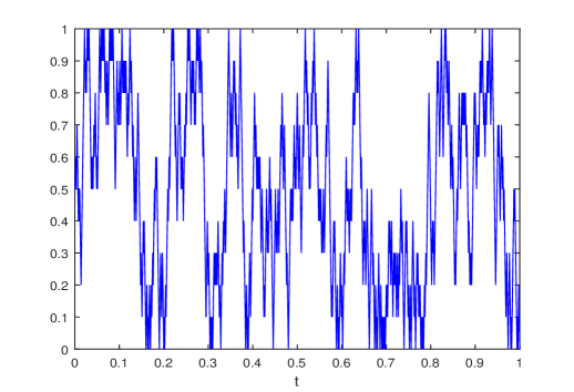
Figure 1: Approximation of optimal solution of problem (16)

III-D Optimal control setting for the multi-battery model

The list of the model parameters and notations
$p(t)$	The production rate
$S(t)$	The current energy price
$\{{\cal F}_{t}\}$	The filtration representing the flow of
	available information
$m$	The number of batteries
$C_{i}$	The capacity of the battery $i$
$y_{i}(t)$	The quantity of the energy currently stored
	in the battery $i$
$\bar{y}_{i}(t)$	The cumulative moving average of $y_{i}(t)$
$u_{i}(t)$	The controlled rate of energy transfer to the
	battery $i$ from the production plant
$[-L_{i},L_{i}]$	The interval of possible values of $u_{i}(t)$
$v_{ij}(t)$	The controlled rate of energy transfer from
	the battery $i$ to the battery $j$
$[-\bar{L}_{ij},\widetilde{L}_{ij}]$	The interval of possible values of $v_{ij}(t)$
${\mathscr{U}}$	The set of ${\cal F}_{t}$-adapted $(u(t),v(t))$ such that
	(9)-(11) holds.
$\alpha_{i}$	The rate of storage losses for the battery $i$
$b_{ij}$	The rate of transfer losses for the energy transfer
	from the battery $i$ to the battery $j$
$\beta_{ij}(v)$	$\beta_{ij}(v)=v$ if $v>0$, and $\beta_{ij}(v)=b_{ij}v$ if $v>0$
${\bf E}$	The expectation
${\mathbb{I}}$	The indicator function

Let a function $\phi:{\bf R}^{n}\times{\bf R}^{n}\times[0,T]$ be selected with the purpose of taking into account the preferences for the battery regimes.

The following stochastic optimal control problem arises: for given $t\in(0,T)$ and $\eta\in\prod_{i=1}^{m}[0,C_{i}]\subset{\bf R}^{m}$,

Maximize

$${\bf E}\int_{t}^{T}\left[\left(p(s)-\sum_{i=1}^{m}u_{i}(s)\right)S(s)+\phi(y(s),\bar{y}(s),s)\right]ds$$

$$+{\bf E}S(T)\sum_{i=1}^{m}y_{i}(T)\quad$$

$$\hbox{over}\quad(u,v)\in{\mathscr{U}},$$

$$\hbox{subject to}\quad\frac{dy_{i}}{ds}(s)=u_{i}(s)-\alpha_{i}y(s)-\sum_{j:\ j\neq i}\beta_{ij}(v_{ij}(s)),$$

$$\quad y_{i}(s)\in[0,C],\quad i=1,...,m,\quad y(t)=\eta.$$ (17)

Here $\bar{y}_{i}(s)\stackrel{{\scriptstyle{\scriptscriptstyle R}}}{{=}}\frac{1}{s}\int_{0}^{s}y_{i}(q)dq$.

Theorem III.1

Problem (17) is equivalent to the problem

Maximize

$${\bf E}\int_{t}^{T}\Biggl{[}\left(p(s)-\sum_{i=1}^{m}u_{i}(s)\right)S(s){\mathbb{I}}_{\{0\leq y_{i}(s)\leq C,\ i=1,...,m\}}$$

$$+\phi(y(s),\bar{y}(s),s)\Biggr{]}ds+{\bf E}S(T)\sum_{i=1}^{m}y_{i}(T)\quad$$

$$\hbox{over}\quad(u,v)\in{\mathscr{U}},$$

subject to

$$\frac{dy_{i}}{ds}(s)=\Bigl{(}u_{i}(s)-\alpha_{i}y(s)$$

$$-\sum_{j:\ j\neq i}\beta_{ij}(v_{ij}(s))\Bigr{)}{\mathbb{I}}_{\{0\leq y_{i}(s)\leq C\}},\quad i=1,...,m,$$

$$\quad y(t)=\eta.\hphantom{5cm}$$ (18)

It can be noted that we do not exclude cases where the process $(p(t),S(t))$. In this case, (18) is a deterministic optimal control problem.

III-E The case of stochastic Markov multi-battery model

In this section, we sssume that $(p(t),S(t))$ is a stochastic Markov diffusion process $\bar{x}(t)$ defined as (3)-(4), and that $\{{\cal F}_{t}\}$ is generated by $w(t)$. Matching of the definitions shows that problem (18) is equivalent to the problem

$$\hbox{Maximize}\quad{\bf E}\left[\int_{t}^{T}h(x(s),u(s),s)ds+\Phi(x(T))\right]\quad$$

$$\hbox{over}\quad(u,v)\in{\mathscr{U}}$$

subject to

$$dx(s)=g(x(s),u(s),v(s),s)ds+\sigma(x(s),s)dw(s),\quad$$

$$x(0)=\eta.$$ (19)

Here $t\in[0,T]$, $x(s)=(x_{1}(s),...,x_{n+2m}(s))^{\top}$, $x_{1}(s)=\bar{x}_{1}(s)=p(s)$, $x_{2}(s)=\bar{x}_{2}(s)=S(s)$, $(x_{n+1}(s),...,x_{n+m}(s))^{\top}=(y_{1}(s),...,y_{m}(s))^{\top}$, $(x_{n+m+1}(s),...,x_{n+2m}(s))^{\top}=(\bar{y}_{1}(s),...,\bar{y}_{m}(s))^{\top}$, $f=(f_{1},...,f_{2m})^{\top}$,

$$\bar{y}(s)=\frac{1}{t}\int_{0}^{s}y(\theta)d\theta,\quad\eta=\left(\begin{array}[]{c}\bar{x}(s)\\ y(s)\\ \bar{y}(s)\end{array}\right)\in{\bf R}^{n+2m},$$

$$\quad x(s)=\left(\begin{array}[]{c}\bar{x}(s)\\ y(s)\\ \bar{y}(s)\end{array}\right),$$

$$g(x,u,s)=\left(\begin{array}[]{c}\bar{g}(x_{1},...,x_{n},s)\\ f(x_{1},...,x_{n},u,v,s)\end{array}\right),\quad$$

$$\sigma(x,u,s)=\left(\begin{array}[]{c}\bar{\sigma}(x_{1},...,x_{n},s)\\ 0_{{\bf R}^{1\times n}}\end{array}\right),$$

$$h(x,u,s)=\Bigl{[}\Bigl{(}x_{1}-\sum_{i=1}^{m}u_{i}\Bigr{)}x_{2}{\mathbb{I}}_{\{0\leq x_{n+i}\leq C,\ i=1,...,m\}}$$

$$+\phi\left(\{x_{n+i}\}_{i=1}^{m},\{x_{n+m+i}\}_{i=1}^{m},t\right)\Bigr{]},$$

$$\Phi(x)=x_{2}\sum_{i=n+1}^{n+m}x_{i},$$

where $x=(x_{1},...,x_{n+2m})^{\top}$,

$$f_{i}(x,u,v,s)=(u_{i}-\alpha_{i}x_{n+i}$$

$$-\sum_{j:\ j\neq i}\beta_{ij}(v_{ij})){\mathbb{I}}_{\{0\leq x_{n+i}\leq C\}},\quad i=1,...,m,$$

$$f_{i}(x,u,v,s)=-s^{-2}x_{n+i}+s^{-1}x_{n+i-m},\quad$$

$$i=m+1,...,2m.$$

IV The dynamic programming approach

The state equations for problems (5) and (19) are degenerate which make them difficult for analysis. In addition, they have discontinuous coefficients. To overcome this last feature, let us approximate the problem as the following. Let continuously twice differentiable functions $I_{\varepsilon,i}:{\bf R}\to[0,1]$ be defined for $\varepsilon>0$ such that $I_{\varepsilon,i}(y)=0$ for $y\notin(0,C_{i})$, $I_{\varepsilon}(y)=1$ for $y\in(\varepsilon,C_{i}-\varepsilon)$, and such that $I_{\varepsilon,i}(y)$ is non-decreasing in $y<\varepsilon$ and $I_{\varepsilon}(y)$ is non-increasing in $y>C_{i}-\varepsilon$.

Let us define $f_{\varepsilon}=(f_{\varepsilon,1},...,f_{\varepsilon,2m})$ and $h_{\varepsilon}$ as

$$f_{\varepsilon,i}(x,u,v,s)=(u-\alpha_{i}x_{n+i}-\sum_{j:\ j\neq i}\beta_{ij}(v_{ij}))I_{\varepsilon}(x_{n+i}),$$

$$h_{\varepsilon}(x,u,s)=\left(x_{1}-\sum_{i=1}^{m}u_{i}\right)x_{2}\prod_{i=1}^{n}I_{\varepsilon,i}(x_{n+i})$$

$$+\phi\left(\{x_{n+i}\}_{i=1}^{m},\{x_{n+m+i}\}_{i=1}^{m},s\right).$$

Let $g_{\varepsilon}$ be defined similarly to $g$ with $f$ replaced by $f_{\varepsilon}$.

The functions $f_{\varepsilon}$ and $h_{\varepsilon}$ approximate functions $f$ and $h$, respectively. In addition, they are continuously differentiable. This allows to apply the dynamic programming approach to the following control problem that approximates the original problem:

$$\hbox{Maximize}\quad{\bf E}\left[\int_{t}^{T}h_{\varepsilon}(x(s),u(s),s)ds+\Phi(x(T))\right]\quad$$

$$\hbox{over}\quad(u,v)\in{\mathscr{U}}$$

subject to

$$dx(s)=g_{\varepsilon}(x(s),u(s),v(s),s)ds+\sigma(x(s),s)dw(s),\quad$$

$$x(0)=x_{0}.$$ (24)

The corresponding optimal value function is

$$J_{\varepsilon}(x,t)\stackrel{{\scriptstyle{\scriptscriptstyle R}}}{{=}}\sup_{(u,v)\in{\mathscr{U}}}{\bf E}\Bigl{\{}\int_{t}^{T}h_{\varepsilon}(x(s),u(s),s)ds$$

$$+\Phi(x(T))\Bigl{|}x(t)=x\Bigr{\}}.$$ (25)

In particular, $J_{0}(x,t)$ is the optimal value function for problem (17); by Theorem III.1, this is also the optimal value function for problem (18) and problem (19).

Let $D={\bf R}^{n+1}\times[0,T]$ for problem (5), and let $D={\bf R}^{n+2m}\times[0,T]$ for problem (19).

Let ${\cal W}$ be the set of continuous functions $w:D\to{\bf R}$ such that there exists $c>0$ such that $|w(x,t)|\leq c(|x|+1)$. Let ${\cal W}_{1}=\{w\in{\cal V}:\,w^{\prime}_{t}\in{\cal W},\,w^{\prime}_{x_{i}}\in{\cal W}\,(\forall i)\}$.

Theorem IV.1

Assume that there are no restrictions (11) (i.e., $R\equiv{\bf R}^{m}\times{\bf R}^{m\times m}$ therein). In this case, For $\varepsilon>0$, the value function $J=J_{\varepsilon}(x,t)$ is a solution of the following Hamilton-Jacobi-Bellman equation

$$J_{t}^{\prime}+\max_{\{u_{i}\},\{v_{ij}\}}\{J_{x}^{\prime}g_{\varepsilon}+h_{\varepsilon}\}+{\scriptstyle\frac{1}{2}}{\rm Tr}\left(\beta^{\top}J_{xx}^{\prime\prime}\beta\right)=0,$$

$$J(x,T)=\Phi(x).$$ (26)

The maximum in the HJB equation is taken over $u=\{u_{i}\}\in{\bf R}^{m}$, $v=\{v_{ij}\}\in{\bf R}^{m\times m}$ such that $u_{i}\in[-L_{i},L_{i}],i=1,...,m$, $v_{ij}\in[-\bar{L}_{ij},\widetilde{L}_{ij}]$, $i,j=1,...,m$, and $(u,v)\in R(x_{1},x_{n+1},...,x_{n+m})$. Boundary value problem (26) has an unique solution in the class of ${\cal W}_{1}$. The HJB equation holds as an equality that is satisfied a.e. for $(x,t)\in D$.

The following theorem establishes the way to approximate the solution $J_{0}$ of the original problem.

Theorem IV.2

The solution $J_{0}$ of the original problem can be approximated as

$$J_{0}(x_{0},0)=\lim_{\varepsilon\to 0}J_{\varepsilon}(x_{0},0).$$ (27)

Hamilton-Jacobi-Bellman equation (26) can be solved via backward calculation after discretization and transition to finite differences; see examples in [3]. However, for a large $n+2m$, numerical implementation will be challenging.

The dimension of the HJB equation is defined by the number of factors used in the model. For example, if $\phi\equiv 0$, $p(t)$ is non-random, and if $S(t)$ can be modelled via a one-dimensional equation, then we can select $n=1$ and $m=0$. In this case, the state space will be two dimensional. Another example: if $m=1$ (i.e. we consider one battery only), and if $(p(t),S(t))$ can be modelled by two dimensional equation, then $n=2$. In this case, the dimension of the state space is $n+2m+1=5$. Note that modelling of energy prices and the production rate is a non-trivial task and may require rather a large number of factors [12].

We address some possible ways to overcome the problem of high dimension in Section V below.

V Pathwise optimization for estimation of the value function

Let $\bar{\mathscr{U}}$ be the class of all pairs $(u(t),v(t))$ of random processes with values in ${\bf R}^{m}\times{\bf R}^{m\times m}$ such that (9)-(11) holds; these processes are not necessarily ${\cal F}_{t}$-adapted, but their values are ${\cal F}_{T}$-measurable, meaning that their path is known for the controller at time $T$.

Let $N=m+m(m+1)/2$, and let us associate a process $(u,v)\in\bar{\mathscr{U}}$ with the $N$-dimensional process $z_{u,v}(t)$ formed as a vector with the components

$$(\{u_{i}(t)\}_{i=1}^{m},\{v_{ij}(t)\}_{i=1,...,m,j=i+1,..,m}).$$

(We excluded the components $\{v_{ij}(t)\}_{i=1,...,m,\,j=1,..,i}$ since they are uniquely defined by $z_{u,v}(t)$ by the restrictions on $v$).

In this section, we assume that the filtration $\{{\cal F}_{t}\}$ is generated by a $N$-dimensional Wiener process $w(t)$. In particular, this case include the stochastic diffusion model described in Section III-E, given that $n=N$.

Let $\Lambda$ be the space of all random processes $\lambda(\cdot)$ such that $\lambda(t)$ is ${\cal F}_{T}$-measurable for all $t\in[0,T]$ and ${\bf E}\int_{0}^{T}\lambda(t)^{2}dt<+\infty$. Let $\Lambda$ be the closure of the set of all processes from $\bar{\Lambda}$ that are $\{{\cal F}_{t}\}$-adapted.

For $\lambda\in\Lambda$ and $k=0,1,2,..$, let

$$M(t)=\int_{0}^{t}\lambda(s)dW(s),\quad\mu(t)=M(T)-M(t),\quad$$

$$\mu^{(0)}=\mu,\quad\mu^{(k)}(t)=-\int_{t}^{T}\mu^{(k-1)}(s)ds.$$

Let $\bar{\mathscr{U}}_{C}$ be the class of all pairs $(u,v)\in\bar{\mathscr{U}}$ such that $y_{i}(t)\in[0,C_{i}]$ almost surely for all $t\in[0,T]$, $i=1,...,m$. Let ${\mathscr{U}}_{C}$ be the class of ${\cal F}_{t}$-adapted pairs $(u,v)\in\bar{\mathscr{U}}_{C}$.

For $(u,v)\in\bar{\mathscr{U}}_{C}$, let us define

$$F(u,v)={\bf E}\int_{t}^{T}\Bigl{[}\left(p(s)-\sum_{i=1}^{m}u_{i}(s)\right)S(s)$$

$$+\phi(y(s),\bar{y}(s),s)\Bigr{]}ds+{\bf E}S(T)\sum_{i=1}^{m}y_{i}(T),$$ (28)

where $y$ and $\bar{y}$ are such as defined in (17).

Let $k\in\{0,1,2,...\}$ be selected, and let

$${\cal L}(u,v,\lambda)={\bf E}F(u,v)+{\bf E}\int_{0}^{T}\mu^{(k)}(t)^{\top}z_{u,v}(t)dt.$$

Theorem V.1

Assume that the function $\phi(y,\bar{y},t)$ is concave in $(y,\bar{y})$, Then

$$\sup_{(u,v)\in{\mathscr{U}}_{C}}{\bf E}F(u,v)=\inf_{\lambda\in\Lambda}\sup_{(u,v)\in\bar{\mathscr{U}}_{C}}{\cal L}(u,v,\lambda).$$ (29)

It can be noted that the assumption on $b_{ij}=0$ above means that the link losses for transmission of energy between batteries are not taken into account.

In Theorem V.1, ${\cal L}$ is an analog of the Lagrangian for the control problem with special constraints that $(u,v)\in{\mathscr{U}}_{C}$.

Theorem V.1 allows to substitute stochastic optimization over the set of adapted controls by the set of non-adapted controls (i.e. controls using the information about the future). This allows to estimate the value function by Monte-Carlo method via simulating $(u,v,\lambda)\in\bar{\mathscr{U}}\times\Lambda$ using approach [1, 5, 7, 11, 23, 9]. Therefore, Theorem V.1 gives an opportunity to estimate how far from optimal is the performance of a particular strategy.

It has to be clarified that an existence of a saddle point does not follow from Theorem V.1; also, this theorem does not give a way to derive an optimal strategy $u$.

VI Proofs

Proof of Theorem II.1. Let $(y(\cdot),u(\cdot))$ be an admissible process for problem (1). It is also an admissible process for problem (2), and the values of the quality criterions for $(y(\cdot),u(\cdot))$ are the same for both problems. Hence the optimal value (i.e., the value of the expectation in the performance criterion for problem (1) is less or equal the the optimal value for problem (2). Further, let $(y(\cdot),\widetilde{u}(\cdot))$ be an admissible process for problem (2). The equation for $y$ in (2) is such that $y(s)\in[0,C]$ for all $t$. In addition, the same $y$ will be generated by the control $\widehat{u}(t)$ such that $\widehat{u}(t)=u(t)$ if $y(t)\in(0,L)$ and $\widehat{u}(t)=\alpha y(t)$ if $y(t)=0$ or $y(t)=L$. It follows that the process $(y(t),\widehat{u}(t))$ is also admissible for problem (1). Furthermore, the control $u$ will not perform better than $\widehat{u}$ because of the presence of the indicator function under the integral in (2). Hence the optimal value (i.e., the value of the expectation in the performance criterion) for problem (2) is less or equal the the optimal value for problem (1). This proves Theorem II.1. $\Box$

The proof of Theorem III.1 is similar.

Proof of Theorem IV.1. Theorem 4.1.1 [18], p.165, implies that $J=J_{\varepsilon}$ satisfies the HJB equation such that it has unique solution in ${\cal W}_{1}$ and all components of $J^{\prime}_{x}$ belong to ${\cal W}$. This HJB equation holds in the sense of an equality of the distributions. Theorem 4.4.3 [18], p.192, implies that $J^{\prime}_{t}\in{\cal V}$ as well. $\Box$.

Proof of Theorem IV.2. Let $(x,t)$ be fixed, and let

$$F_{\varepsilon}(u,v)={\bf E}\Bigl{\{}\int_{t}^{T}h_{\varepsilon}(x(s),u(s),s)ds+\Phi(x(T))\Bigr{)},$$

where $(u,v)\in{\mathscr{U}}$, and where $x$ is the corresponding solution of the differential equation in (19).

Let $\delta>0$, and let $(\widehat{u},\widehat{v})$ be such that $F_{0}(\widehat{u},\widehat{v}))\geq J_{0}(x,t)-\delta/2$. Let $\widehat{y}(t)$ be the corresponding vector process. Let $\widehat{u}_{\varepsilon}=\{\widehat{u}_{\varepsilon,i}\}$ and $\widehat{v}_{\varepsilon}=\{\widehat{v}_{\varepsilon,ij}\}$ be such that $\widehat{u}_{\varepsilon,i}(t)=\widehat{u}_{i}(t)$ and $\widehat{v}_{\varepsilon,ij}(t)=\widehat{v}_{ij}(t)$ if $\widehat{y}_{i}(t)\in(\varepsilon,C-\varepsilon)$, and where $\widehat{u}_{\varepsilon,i}(t)=\alpha_{i}\widehat{y}_{i}(t)$ and $\widehat{v}_{\varepsilon,ij}(t)=\widehat{v}_{\varepsilon,ji}(t)=0$ if $\widehat{y}_{i}(t)\in\{\varepsilon,C-\varepsilon\}$. We have that there exists $\varepsilon>0$ such that $F(\widehat{u}_{\varepsilon},\widehat{v}_{\varepsilon})\geq F(\widehat{u},\widehat{v})-\delta/2$. Therefore, for an arbitrarily small $\delta>0$, one can find $(\widehat{u}_{\varepsilon},\widehat{v}_{\varepsilon})$ such that $F(\widehat{u}_{\varepsilon},\widehat{v}_{\varepsilon})\geq F(\widehat{u},\widehat{v})-\delta\geq J_{0}(x,t)-\delta/2$. Then the proof follows. $\Box$

Proof of Theorem V.1. It can be shown that $M(t)={\bf E}\{M(T)|{\cal F}_{t}\}$ (i.e., this is the conditional expectation given ${\cal F}_{t}$). Similarly to the proof of Theorem 4.1 [9], we obtain that $(u,v)\in\bar{\mathscr{U}}_{C}$ belongs to $\mathscr{U}_{C}$ if and only if

$${\bf E}\int_{0}^{T}\mu(t)^{\top}z^{(k)}(t)dt={\bf E}\int_{0}^{T}\mu^{(k)}(t)^{\top}z(t)dt=0$$

for any $k\geq 0$ and any $\lambda\in\Lambda$. Here $z^{(0)}=z_{u,v}$, $z^{(k)}(t)=\int_{0}^{t}z^{(k-1)}(s)ds$, $k=1,2,3,...$. This is why ${\cal L}(u,v,\lambda)$ can be used as a Lagrangian for the problem with the constraint that $(u,v)\in{\mathscr{U}}_{C}$.

Further, the set $\bar{\mathscr{U}}_{C}$ is convex and closed in the square integral metric. By the assumtions on $b_{ij}$, we have that $y$ and $\bar{y}$ depend linearly on $(u,v)\in\bar{\mathscr{U}}_{C}$. By the assumptions on $\phi$, the function $F(u,v)$ is concave on $\bar{\mathscr{U}}_{C}$. Then the proof of Theorem V.1 follows The statement of the theorem follows Propositions 1.2 and 2.3 [10], Chapter 4, similarly to the proof of Theorem 4.1 [9]. $\Box$

VII Conclusion

The paper suggests a compact and yet comprehensive model for decision making under uncertainty for a of small or medium producer of energy operated a plant and a system of batteries. The problem setting takes into account the topology of the system of batteries and losses for transferring and storage of energy. A method of calculating an optimal operating algorithm for storing and dispatching strategy is suggested. The optimality is defined by a performance criterion that takes into account the expected monetary return for the producer. In addition, the performance criterion takes into account preferable regimes for batteries charging and discharging that may help to prolong the battery life.

The model includes two processes that cannot be controlled by the operator: the production rate $p(t)$ and the energy price $S(t)$. If these processes are predictable, then calculation of the optimal strategy requires to solve a multi-dimensional deterministic optimal control problem. The paper is focused on the setting where processes $p(t)$ and $S(t)$ are random, currently observable, and unpredictable, with known stochastic evolution law. This leads to a multi-dimensional stochastic optimal control problem. A method of solution is developed for the model where $(p(t),S(t))$ is part of stochastic Markov diffusion process. There are no restrictions on the choice of the parameters of this diffusion process; in this sense, the model is very general. In particular, this methods is also applicable for the case where the process $(p(t),S(t))$ is non-random.

The Markov diffusion models are quite common in engineering and economics; their main restriction is that they use continuous processes without jumps. The model introduced in this paper is quite flexible and allow many modifications that were not executed in the present paper to avoid overloading by technical details.

Instead of the diffusion Markov model described in Section III, many other stochastic models can be accommodated for the dynamics of $(p(t),S(t))$. For example, the dynamic programming method can be extended on the jump diffusion model using the approach [21]. A case of general right-continuous processes $(p,S)$ could be considered similarly to [2] The continuous time model could be replaced by a discrete time model. We leave this for the future research.

Potentially, uncertainty can be taken into account with stochastic models replaced by interval type uncertainty. We leave this for the future research as well.

In the present form, the model is based on the continuous time processes. However, this is rather technical assumption since a similar discrete time model can be obtained via straightforward discretization.

Numerical implementation of the suggested method would require time discretization and backward solution of the dynamic programming equation. However, the state space dimension for this equation will be high for a large number of factors arising in a multi-battery setting. This means that numerical solution could require significant computational efforts. To partially address this, we suggest to estimate of the optimal value function using the pathwise optimization approach. We leave further development of the numerical methods for the future research.

Usually, decision making in the stochastic framework relies on forecasting the underlying processes. In stochastic evolution models such as (3)-(4), the forecasting is assumed in an implicit form: a model implies forecasts for the underlying processes, for example, the conditional expectations of the future values given the observations. These forecasts and the corresponding errors can be calculated analytically for a particular model such as (3)-(4). One would need to apply statistical inference and forecasting methods to calibrate the parameters for a model. However, this requires special consideration beyond the scope of this paper. We leave this for the future research.

Several other important factors have been left for the future research. Possible cooperation with the grid operators and other producers could be included in the model. Some restrictions on batteries could be imposed, for example, on simultaneous charging or discharging. It would be interesting to consider the problem of optimal selection of the topology of the system of batteries to minimize the losses.

References

- [1] Bender, C., Schoenmakers, J., Zhang, J. (2015). Dual representations for general multiple stopping problems. Mathematical Finance 25, Issue 2, 339-370.
- [2] Bender, C. and Dokuchaev, N. (2017). A first-order BSPDE for swing option pricing: Classical solutions. Mathematical Finance 27(3), 902–925.
- [3] Benth, F. E., Lempa, J., Nilssen, T. K. (2011): On the optimal exercise of swing options in electricity markets. Journal of Energy Markets 4, 3–28.
- [4] Breton S., Moe G. (2009). Status, plans and technologies for offshore wind turbines in Europe and North America, Renewable Energy 34 (3) 646–654.
- [5] Brown, D. B., Smith, J. E., Sun, P. (2010): Information relaxations and duality in stochastic dynamic programs. Oper. Res. 58, 785–801.
- [6] Choobineh, M ; Mohagheghi, S. (2019). Robust optimal energy Pricing and dispatch for a multi-microgrid industrial park operating based on Just-in-Time strategy. IEEE Transactions on Industry Applications, 65(4), 3321–3330.
- [7] Davis, M.H.A., Burstein, G. (1992). A deterministic approach to stochastic optimal control with application to anticipative control. Stochastics, v.40, 203–256.
- [8] Dincer F. (2001), The analysis on photovoltaic electricity generation status, potential and policies of the leading countries in solar energy, Renewable and Sustainable Energy Reviews 15 (1), 713-720.
- [9] Dokuchaev, N. (2017). First Order BSPDEs in higher dimension for optimal control problems. SIAM Journal on Control and Optimization 55 (2), 818-834.
- [10] Ekland, I., Temam, R. (1999). Convex Analysis and Variational Problems. SIAM, Philadelphia.
- [11] Haugh, M., Kogan, L. (2004). Pricing American options: a duality approach. Operations Research 52, 258–270.
- [12] Hinz, J. 2003, Modelling day-ahead electricity prices, Applied Mathematical Finance 10, no. 2, pp. 149-161.
- [13] Hoffert, M.I., K. Caldeira K., Benford G., Criswell D. R., Green C., Herzog H., Jain A.K., Kheshgi H.S., K. S. Lackner K.S. , Lewis J.S., et al. (2002). Advanced technology paths to global climate stability: Energy for a greenhouse planet, Science 298 (5595) 981–987.
- [14] Khalid M., Savkin A.V., and Agelidis V.G. (2015). An adaptive control algorithm for wind power dispatch using a battery energy storage system. Proceedings of the IEEE Multi-Conference on Systems and Control, Sydney, Australia, September 2015.
- [15] Khalid M., Savkin A.V. (2012). A method for short-term wind power prediction with multiple observation points, IEEE Trans. Power Syst., vol. 27, no. 2, pp. 579–586.
- [16] Koller M., Borsch T., Ulbig A., Andersson G. (2013). Defining a degradation cost function for optimal control of a battery energy storage system: PowerTech (POWERTECH), 2013 IEEE Grenoble. 16-20 June 2013, pp. 1–6.
- [17] Kim J.H, Powell W. B. (2011). Optimal energy commitments with storage and intermittent supply, Operations Research 59 (6) 1347-1360.
- [18] Krylov, N.V. (1980). Controlled Diffusion Processes. Springer-Verlag, New York.
- [19] Ning, G., Ralph E., White R.E., Popov, B.N. A generalized cycle life model of rechargeable Li-ion batteries. (2006). Electrochimica Acta 51, 2012–2022.
- [20] O’Connor, M., Lewis T., Dalton G. (2013) Operational expenditure costs for wave energy projects and impacts on financial returns. Renewable Energy 50, 1119–1131.
- [21] Øksendal, B., Sulem, A. (2007). Applied Stochastic Control of Jump Diffusions. Springer, Berlin-Heidelberg.
- [22] Oudalov A, Chartouni D., and Ohler C., (2007). Optimizing a battery energy storage system for primary frequency control, IEEE Transactions on Power Systems, vol. 22, no. 3, pp. 1259–1266.
- [23] Rogers, L. C. G. (2007). Pathwise stochastic optimal control. SIAM J. Control Optim. 46, 1116–1132.
- [24] Schoenmakers, J. (2012). A pure martingale dual for multiple stopping. Finance Stoch. 16, 319-334.
- [25] Teleke S., Baran M., Bhattacharya S., and Huang A. (2010). Optimal control of battery energy storage for wind farm dispatching. IEEE Transactions on Energy Conversion, vol. 25, no. 3, 787–794.
- [26] Worighi, I., Maach, A., Hafid, A., Hegazy, O.,Van Mierlo, J. (2019). Integrating renewable energy in smart grid system: Architecture, virtualization and analysis 18, 100226.
- [27] Xie L., Gu Y., Eskandari A., and Ehsani M. (2012). Fast MPC-based coordination of wind power and battery energy storage systems. Journal of Energy Engineering, vol. 138, pp. 43–53.