Optimal Triangulation of Saddle Surfaces

Abstract

We consider the piecewise linear approximation of saddle functions of the form $f(x,y)=ax^{2}-by^{2}$ under the $L_{\infty}$ error norm. We show that interpolating approximations are not optimal. One can get slightly smaller errors by allowing the vertices of the approximation to move away from the graph of the function.

1 Introduction

We are given the bivariate quadratic function

$$f(x,y)=ax^{2}+2bxy+cy^{2}+dx+ey+g,$$ (1)

and we want to approximate it with a piecewise linear function $\hat{f}(x,y)$ which is as simple as possible. More precisely, the function $\hat{f}$ that we are looking for is defined by a triangulation $\mathcal{T}$ of the plane and the values $\hat{f}(x,y)$ at the vertices $(x,y)$ of the triangulation. We want to minimize the number of triangles. The error criterion that we consider is the $L_{\infty}$ distance or vertical distance (thinking geometrically in the three-dimensional space where the graph of $f$ lives); it should be bounded by some specified parameter $\varepsilon$:

$$\max_{x,y}|f(x,y)-\hat{f}(x,y)|\leq\varepsilon$$

For simplicity, we will let $(x,y)$ range over the whole plane. Thus, we cannot just count the triangles. We rather minimize the triangle density. Let $Q_{r}=[-r/2,r/2]\times[-r/2,r/2]$ be the $r\times r$ square centered at the origin. The triangle density counts the number of triangles $T\in\mathcal{T}$ of the triangulation that intersect the squares $Q_{r}$ for larger and larger side length $r$, in comparison to the area of these squares:

$$\limsup_{r\to\infty}\frac{|\{\,T\in\mathcal{T}\mid T\cap Q_{r}\neq\emptyset\,\}|}{r^{2}}$$

We have three cases:

1. $f$ is a positive or negative definite quadratic function; in other words, $f$ is convex or concave.

2. $f$ is indefinite; the graph of $f$ is a saddle surface, and it has negative Gauss curvature.

3. $f$ is semidefinite; its graph is a parabolic cylinder.

The cases can be distinguished by the discriminant $ac-b^{2}$ being positive, negative, or zero.

Case 1 is easy; the classical theory of piecewise linear convex approximation applies. We will mention the respective results below. Case 3, as well as the case of a linear function ($a=b=c=0$), is a boundary case, and we will not treat it. We will concentrate on Case 2, which is representative of negatively curved surfaces in 3 dimensions:

Theorem 1.1

If $f$ is indefinite $(ac-b^{2}<0)$, then there is a piecewise linear function $\hat{f}$ approximating $f$ with vertical error $\varepsilon$ that has triangle density

$$\frac{\sqrt{3}}{4}\cdot\sqrt{b^{2}-ac}\cdot\frac{1}{\varepsilon}\approx 0.43301\cdot\sqrt{b^{2}-ac}\bigm{/}\varepsilon.$$

The triangulation consists of a grid of congruent triangles like in Figure 1. This grid can be freely translated in the plane, and in addition, there is a one-parameter family of solutions of different shapes with the same properties.

If we require an interpolating approximation, the error of the approximation is slightly larger, as stated in the following theorem. Here, the vertices of $\hat{f}$ are constrained to lie on the given surface, i.e., $\hat{f}(x,y)=f(x,y)$ for all vertices $(x,y)$ of the triangulation.

Theorem 1.2

If $f$ is indefinite $(ac-b^{2}<0)$, then there is a piecewise linear interpolating function $\hat{f}$ approximating $f$ with vertical error $\varepsilon$ that has triangle density

$$\frac{1}{\sqrt{5}}\cdot\sqrt{b^{2}-ac}\cdot\frac{1}{\varepsilon}\approx 0.44721\cdot\sqrt{b^{2}-ac}\bigm{/}\varepsilon,$$

and this bound is best possible.

This theorem is due to Pottmann, Krasauskas, Hamann, Joy, and Seibold (2000), except that the explicit error bound is not stated there. For comparison, we state the well-known result for convex functions (see Pottmann et al. 2000, for example):

Theorem 1.3

If $f$ is strictly convex or strictly concave $(ac-b^{2}>0)$, then there is a piecewise linear function $\hat{f}$ approximating $f$ with vertical error $\varepsilon$ that has triangle density

$$\frac{2}{\sqrt{27}}\cdot\sqrt{ac-b^{2}}\cdot\frac{1}{\varepsilon}\approx 0.38490\cdot\sqrt{ac-b^{2}}\bigm{/}\varepsilon.$$

If $\hat{f}$ is required to be interpolating, the bound becomes

$$\frac{4}{\sqrt{27}}\cdot\sqrt{ac-b^{2}}\cdot\frac{1}{\varepsilon}\approx 0.76980\cdot\sqrt{ac-b^{2}}\bigm{/}\varepsilon.$$

These bounds are best possible.

Figure 1: A triangular grid

As in Theorem 1.1, the triangulations in Theorems 1.2 and 1.3 are triangular grids, and the statement about the translations and the one-parameter family of solutions holds likewise.

In contrast to Theorems 1.2 and 1.3, we do not know whether the constant in Theorem 1.1 is best possible.

For an infinite grid like in Figure 1, the number of vertices per area is half the number of triangles. Thus, in order to get estimates for the vertex density, just divide the bounds in the theorems by 2.

Our main result, Theorem 1.1, will be proved in Section 3.2, after reproving Theorem 1.2 in Section 3.1. For comparison, Section 2 treats the convex case (Theorem 1.3). The remainder of this introduction will motivate the problem and prepare it for the solution.

1.1 Vertical distance and quadratic functions

There are two reasons why we have chosen to concentrate (i) on quadratic functions and (ii) on the vertical distance:

1. the relevance from the viewpoint of applications, and

2. the mathematical simplicity that comes with this model and which allows us to derive clean results.

We will discuss these aspects now.

1.1.1 Applications and related work

Piecewise linear approximation is a fundamental problem in converting some general function or shape into a form that can be stored and processed in a computer. Our original motivation comes from the desire to approximate the boundaries of three-dimensional configuration spaces for robot motion planning (Atariah, 2014; Atariah, Ghosh, and Rote, 2013), which turn out to be ruled surfaces with negative Gauss curvature.

Of course, when approximating a surface in space, one does not want to use the vertical distance but rather something like the Hausdorff distance, which measures the distance from the given surface to the nearest point of the approximating surface, in a direction perpendicular to one of the surfaces. However, if we consider a small patch of the surface and we look for a good approximation in a local neighborhood, we can rotate the surface in 3-space such that it becomes horizontal. Then, as long as the surface does not curve to much away from the horizontal direction, the vertical distance is a good substitute for the Hausdorff distance, and it is always an upper bound on it.

For piecewise linear approximation, the first interesting terms of the Taylor approximation are the quadratic terms. Thus, quadratic functions are the model of choice for investigating the question of best approximation.

Every smooth function can be approximated by a quadratic function in some neighborhood, and the same is true for surfaces. In this sense, our results are applicable as a local model, for a smooth surface or a smooth function as the approximation gets more and more refined. This approach has been pioneered in the above-mentioned paper of Pottmann et al. (2000). Our contribution is to improve the result for non-interpolating approximation of saddle surfaces.

Bertram, Barnes, Hamann, Joy, Pottmann, and Wushour (2000) have extended this approach to an arbitrary bivariate function $f$, by taking optimal local approximations on suitably defined patches and “stitching” them together at the patch boundaries. (The setting of this paper is actually somewhat different: the bivariate function $f$ is given as a set of scattered data points.)

In arbitrary dimensions, the problem of optimal piecewise linear approximation has been adressed by Clarkson (2006), without deriving explicit constant factors. For convex functions and convex bodies, there is a vast literature on optimal piecewise linear approximation in many variations, see for example the treatment in Pottmann et al. (2000) and the references given there.

1.1.2 Mathematical properties; transforming the problem into normal form

One crucial property of a quadratic function is that, from the point of view of our problem, it “looks the same” everywhere. This is made precise in the following observation.

Lemma 1

Let $f$ be a quadratic function

$$f(x,y)=ax^{2}+2bxy+cy^{2}+dx+ey+g,$$ (1)

and let $(x_{1},y_{1}),(x_{2},y_{2})\in\mathbb{R}^{2}$ be two points. Then there is an affine transformation of $\mathbb{R}^{3}$ that

1. maps the graph of $f$ to itself,

2. maps the point $(x_{1},y_{1},f(x_{1},y_{1}))$ to the point $(x_{2},y_{2},f(x_{2},y_{2}))$,

3. maps vertical lines to vertical lines,

4. leaves vertical distances between points on the same vertical line unchanged,

5. acts as a translation in the plane when the $z$-coordinate is ignored.

Proof

We construct a transformation of the form

$$\begin{pmatrix}x\\ y\\ z\end{pmatrix}\mapsto\begin{pmatrix}x^{\prime}\\ y^{\prime}\\ z^{\prime}\end{pmatrix}=\begin{pmatrix}1&0&0\\ 0&1&0\\ u&v&1\end{pmatrix}\begin{pmatrix}x\\ y\\ z\end{pmatrix}+\begin{pmatrix}x_{2}-x_{1}\\ y_{2}-y_{1}\\ w\end{pmatrix}$$

for some parameters $u,v,w$ that are to be determined. It is evident that the points $(x_{0},y_{0},z)$ on a vertical line, for fixed $x_{0},y_{0}$, are mapped to points $(\bar{x},\bar{y},\bar{z}+z)$, for some fixed $\bar{x},\bar{y},\bar{z}$, and thus, Properties 3 and 4 are fulfilled. Moreover, when restricted to the first two coordinates, the transformation acts as a translation on the $xy$-plane (Property 5), moving $(x_{1},y_{1})$ to $(x_{2},y_{2})$. Thus, Property 2 holds provided that we can show Property 1. Property 1 requires that $f(x,y)=z$ implies $f(x^{\prime},y^{\prime})=z^{\prime}$. This is fulfilled by setting $u=2a(x_{2}-x_{1})+2b(y_{2}-y_{1})$, $v=2b(x_{2}-x_{1})+2c(y_{2}-y_{1})$, and $w=f(x_{2}-x_{1},y_{2}-y_{1})-g$, as is easily checked by calculation. ∎

The problem of finding a best approximation remains also unchanged when adding a linear function to $f$. This means that we can assume that $d=e=g=0$ in (1). By a principal axis transform, the $xy$-plane can be rotated such that $f$ gets the form $f(x,y)=a^{\prime}x^{2}+c^{\prime}y^{2}$, with $a^{\prime}c^{\prime}=ac-b^{2}$. Finally, we scale the $x$-and $y$-axis by $\sqrt{|a^{\prime}|}$ and $\sqrt{|c^{\prime}|}$ such that $f$ becomes

$$f(x,y)=\pm x^{2}\pm y^{2}.$$

The area is changed by the factor $\sqrt{|a^{\prime}c^{\prime}|}=\sqrt{|ac-b^{2}|}$, and this is taken into account by the corresponding factor in Theorems 1.1–1.3.

1.2 Covering the plane with copies of a triangle

Now we show that a triangle where all three vertices have the same fixed offset $\Delta$ from the surface $f$ can be used to construct a global approximation. The offset $\Delta$ can be positive or negative. The case $\Delta=0$ corresponds to interpolating approximation.

Lemma 2

Let $T=p_{1}p_{2}p_{3}$ be a triangle in the plane with area $A$, and let $\hat{f}$ be a linear function such that $\hat{f}(p_{i})=f(p_{i})+\Delta$ for the three vertices $p_{i}$ of $T$. Let $\varepsilon$ denote the maximal vertical distance within the triangle: $\varepsilon:=\max\{\,|\hat{f}(x,y)-f(x,y)|:(x,y)\in T\,\}$.

Then there is a piecewise linear approximation of $f$ over the whole plane with vertical distance $\varepsilon$ and triangle density $1/A$.

Proof

If we rotate the triangle $T$ by $180^{\circ}$ about the origin, we can define a linear function over the rotated triangle $T^{\prime}$ with the same maximum error $\varepsilon$. Translates of $T$ and $T^{\prime}$ can be used to tile the plane as in Figure 1. By Lemma 1, defining a linear function over any translate of $T$ or $T^{\prime}$ with the same vertex offset $\Delta$ leads to an error of $\varepsilon$ over this triangle. Since all offsets are equal, the triangles fit together to form a piecewise linear interpolation over the whole plane. The triangle density is $1/A$. ∎

If we impose the condition that all vertices have the same vertical offset from the surface $f$, this lemma turns the problem of finding an approximating triangulation with few triangles into the problem of finding a largest-area triangle $T$ subject to the error bound.

2 Convex surfaces

After these preparations, it is easy to solve the convex case $f(x,y)=x^{2}+y^{2}$. Consider first the case of interpolating approximation. The largest error over a triangle $T$ is assumed at the center of the smallest enclosing circle $C$, see Figure 2:

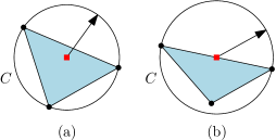
Figure 2: The smallest enclosing circle $C$ for (a) an acute triangle, (b) an obtuse triangle

This can be seen easily when the center of $C$ is at the origin, which we can assume by Lemma 1. Let $r$ be the radius of $C$. Then the line or plane through the points of maximum distance from the origin lies at height $z=r^{2}$, giving rise to an error of $\varepsilon=r^{2}$. The search for an optimal triangle thus amounts to finding a largest-area triangle inside a circle of radius $\sqrt{\varepsilon}$. This is clearly an equilateral inscribed triangle, and its area is $\varepsilon\frac{3\sqrt{3}}{4}$. By Lemma 2, this leads to the second part of Theorem 1.3.

It is obvious that the optimal triangle is not unique: it can be rotated freely, giving rise to a one-parameter family of optimal triangulations.

The non-interpolating case is now easily derived from the interpolating case, because for a convex function, an interpolating approximation $\hat{f}$ cannot lie below $f$. Thus, finding an interpolating approximation amounts to looking for a function $\hat{f}$ that satisfies

$$f(x,y)\leq\hat{f}(x,y)\leq f(x,y)+\varepsilon$$ (2)

for all $x,y$, see Figure 3. To see that the problems are indeed equivalent, observe that any function $\hat{f}$ fulfilling (2) can be turned into an interpolating approximation by reducing the values $\hat{f}(x,y)$ at each vertex $(x,y)$ of the triangulation to its lower bound, namely $f(x,y)$, without violating (2). On the other hand, non-interpolating approximation looks for a function that satisfies

$$f(x,y)-\varepsilon\leq\hat{f}(x,y)\leq f(x,y)+\varepsilon.$$

A non-interpolating approximation with error $\varepsilon$ can thus be obtained from an interpolating approximation $\hat{f}$ with error $2\varepsilon$ by subtracting $\varepsilon$ from $\hat{f}$, and vice versa.

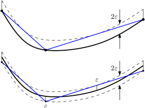
Figure 3: A non-interpolating approximation corresponds to an interpolating approximation with a doubled error bound.

3 Saddle surfaces

For the indefinite case, it is more convenient to rotate the coordinate system by $45^{\circ}$ and consider the function in the form

$$f(x,y)=2xy.$$

Lemma 3

The maximum vertical error between $f(x,y)$ and a linear function $\hat{f}(x,y)=ux+vy+w$ over a triangular region $T$ is never attained in the interior of $T$.

Proof

A local maximum of the error $|f(x,y)-f(x,y)|=\max\{f(x,y)-\hat{f}(x,y),\,\hat{f}(x,y)-f(x,y)\}$ must be a local maximum of the function $f(x,y)-\hat{f}(x,y)$ or of $\hat{f}(x,y)-f(x,y)$. However, these functions are saddle functions and they cannot have a local extremum in the interior of $T$. More formally, they have, respectively, the Hessians $\left(\begin{smallmatrix}0&2\\ 2&0\end{smallmatrix}\right)$ and $\left(\begin{smallmatrix}0&-2\\ -2&0\end{smallmatrix}\right)$, which are not negative semidefinite, and thus the second-order necessary condition for a local maximum is not fulfilled. ∎

We conclude that it suffices to measure the approximation error on the edges and vertices of $T$.

3.1 Interpolating approximation

We will first treat the interpolating case and recover the results of Pottmann et al. (2000) (our Theorem 1.2) as a preparation for the free approximation (Theorem 1.1) in Section 3.2. The error along a chord connecting two points of the surface can be evaluated very easily.

Lemma 4

(Pottmann et al., 2000, Lemma 2) Let $p,q\in\mathbf{R}^{2}$ be two points. The maximum vertical error between $f$ and the linear interpolation between $f(p)$ and $f(q)$ is attained at the midpoint $(p+q)/2$ and its value is

$$\max_{0\leq\lambda\leq 1}|(1-\lambda)f(p)+\lambda f(q)-f((1-\lambda)p+\lambda q)|=\frac{|f(q-p)|}{4}.$$ (3)

Proof

By Lemma 1, we may translate the plane such that $p$ becomes the origin. Then the function $f$ along the segment $pq$ is simply the quadratic function $f((1-\lambda)p+\lambda q)=\lambda^{2}f(q)$, for which the statement is easy to establish, see Figure 4. ∎

Figure 4: Approximation of a quadratic function by a chord

In the convex case $f(x,y)=x^{2}+y^{2}$ of Section 2, it was clear that there is a one-parametric solution space, since the function is rotationally symmetric. In the saddle case, it comes somewhat as a surprise that the optimal triangulations have a similar variability. However, this is explained by the pseudo-Euclidean transformations, which have the form

$$(x,y)\mapsto(mx,y/m),$$

for a parameter $m\neq 0$, and which leave the graph of the function $f$ invariant, see Pottmann et al. (2000). They scale the $x$- and $y$-coordinates, but they preserve the area. We will make use of the freedom to apply pseudo-Euclidean transformations to simplify the calculations.

Let us now look for the largest-area triangle $p_{1}p_{2}p_{3}$ such that the maximum error on each edge $p_{1}p_{2}$, $p_{2}p_{3}$, and $p_{1}p_{3}$, as computed by (3), is bounded by $\varepsilon$. In more explicit terms, this means that

$$|f(p_{i}-p_{j})|=|2(x_{i}-x_{j})(y_{i}-y_{j})|\leq 4\varepsilon.$$ (4)

We shall show that these constraints must hold as equalities, because of the concave nature of the constraints.

Lemma 5

In a triangle of maximum area subject to the constraints (4), each triangle edge must fulfill this constraint as an equality.

Proof

Let us consider $p_{1}$ and $p_{2}$ as fixed and maximize the area by varying $p_{3}$ subject to the constraints (4). We will show that both constraints that involve $p_{3}$ must be tight. The lemma then follows by applying the same argument to $p_{1}$ instead of $p_{3}$.

The area is a linear function of $p_{3}$, proportional to the distance of $p_{3}$ from the line $p_{1}p_{2}$. If none of the two constraints involving $p_{3}$ is tight, we can freely move $p_{3}$ in some small neighborhood, and hence this situation cannot be optimal.

Suppose now that the constraint for one edge incident to $p_{3}$, say, $p_{1}p_{3}$, is tight but the other one, $p_{2}p_{3}$, is fulfilled as a strict inequality. The constraint (4) for $p_{1}p_{3}$ confines $p_{3}$ within a region $R$ bounded by four hyperbola branches centered at $p_{1}$, shown in Figure 5a.

(a)   (b)

Figure 5: The feasible region $R$ is bounded by four hyperbola branches.

This region is strictly concave in the following sense: Through each point $p_{3}\in R$, there is a line segment $s$ in $R$ that contains $p_{3}$ in its interior. (When $p_{3}$ lies on the boundary of $R$, as we are assuming, $s$ is a part of the tangent to the boundary at this point.) Moreover, all points of $s$ other than $p_{3}$ lie in the interior of $R$. Now, we can move along $s$ by some small amount in at least one direction without decreasing the area function, such that, in the resulting point, none of the two constraints involving $p_{3}$ is tight. But this was already excluded above. ∎

We can classify triangle edges $p_{i}p_{j}$ into ascending edges (extending in the SW–NE direction) and descending edges (extending in the NW–SE direction), according to the sign of $(x_{j}-x_{i})(y_{j}-y_{i})$. Let us assume without loss of generality that the predominant category is ascending, and two ascending edges are $p_{1}p_{2}$ and $p_{1}p_{3}$. Furthermore, by Lemma 1, we can assume that $p_{1}$ is at the origin, and, after a rotation by $180^{\circ}$ if necessary, $p_{2}$ and $p_{3}$ lie in the first quadrant, see Figure 6a.

Figure 6: (a) The potential positions of $p_{2}$ and $p_{3}$. (b) Transforming the triangle by pseudo-Euclidean motions.

The two points $p_{2}=(x_{2},y_{2})$ and $p_{3}=(x_{3},y_{3})$ lie on the hyperbola $xy=2\varepsilon$. By applying a pseudo-Euclidean transformation, it suffices to consider the case that they lie symmetric with respect to the line $x=y$, i.e., $(x_{3},y_{3})=(y_{2},x_{2})$. We now substitute this and the equation $y_{2}=2\varepsilon/x_{2}$ into the relation (4) for $|f(p_{3}-p_{2})|$ and obtain the equation $|f(p_{3}-p_{2})|=|2(x_{3}-x_{2})(y_{3}-y_{2})|=|2(y_{2}-x_{2})(x_{2}-y_{2})|=2(y_{2}-x_{2})^{2}=2(2\varepsilon/x_{2}-x_{2})^{2}=4\varepsilon$. Solving for $x_{2}$ gives $p_{2}=(\sqrt{\varepsilon/2}(\sqrt{5}+1),\sqrt{\varepsilon/2}(\sqrt{5}-1))$. (The quartic equation for $x_{2}$ has four solutions in total. There is another nonnegative solution, which just swaps the two coordinates $x_{2}$ and $y_{2}$, or equivalently, swaps $p_{2}$ with $p_{3}$. The other two solutions are just the negations of the first two.) The area of the triangle $p_{1}p_{2}p_{3}$ is

$$\frac{1}{2}\left|\begin{matrix}x_{2}&x_{3}\\ y_{2}&y_{3}\\ \end{matrix}\right|=\frac{1}{2}\left|\begin{matrix}x_{2}&y_{2}\\ y_{2}&x_{2}\\ \end{matrix}\right|=\tfrac{1}{2}(x_{2}^{2}-y_{2}^{2})=\tfrac{1}{2}(x_{2}+y_{2})(x_{2}-y_{2})=\varepsilon\sqrt{5}.$$ (5)

By Lemma 2, this establishes Theorem 1.2. ∎

The one-parameter family of triangulations that are optimal is obtained by applying pseudo-Euclidean transformations to the symmetric solution $p_{1}p_{2}p_{3}$ computed above, see Figure 6b: The set of optimal triangles consists of all triangles $p_{1}p_{2}p_{3}$ with $p_{1}=(0,0)$, $p_{2}=(\sqrt{\varepsilon/2}(\sqrt{5}+1)\cdot m,\sqrt{\varepsilon/2}(\sqrt{5}-1)/m)$, and $p_{3}=(\sqrt{\varepsilon/2}(\sqrt{5}-1)\cdot m,\sqrt{\varepsilon/2}(\sqrt{5}+1)/m)$, for $m\neq 0$, as well as their reflections in the coordinate axes and their translations.

We can use this freedom to choose a triangulation which optimizes some secondary criterion, like the shape of the triangles. Atariah (2014, Chapter 3) considered the problem of maximizing the smallest angle. He showed that the optimal triangle is, not surprisingly, always an isosceles triangle. In general, there are two different shapes of isosceles triangles, corresponding to the two patterns in Figure 7a–b. For a general quadratic function, these two cases have differently shaped triangles, and the best choice depends on the ratio between the eigenvalues of the quadratic form associated to $f$.

The family of optimal triangulations that are characterized above is somewhat counter-intuitive: The surface described by $z=2xy$ is a ruled surface: it is swept out by a line. Any edge between two points on a line of the ruling has error 0, no matter how long it is. It seems attractive to use edges that go along the ruling. The above results show that this is not the best idea: it is better to “distribute” the error evenly to the three edges. If one wants to insist on following the ruling, one can impose that $p_{2}$ lies on the $x$-axis. The optimal triangle is then an isosceles triangle $p_{1}p_{2}p_{3}$ with a base $p_{1}p_{2}$ of arbitrary length and $p_{3}$ on the hyperbola $|xy|=2\varepsilon$, and its area is $2\varepsilon$ instead of $\varepsilon\sqrt{5}$.

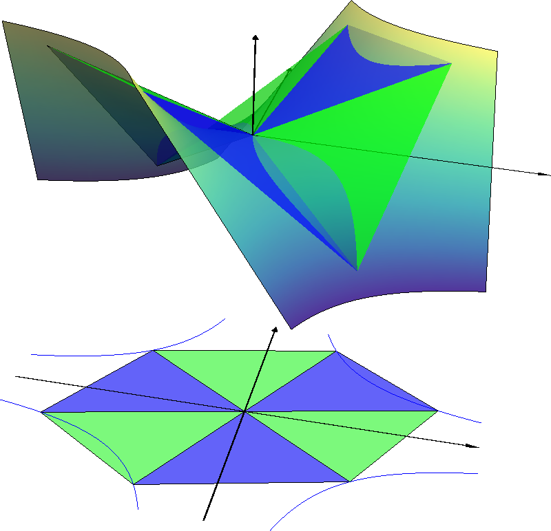
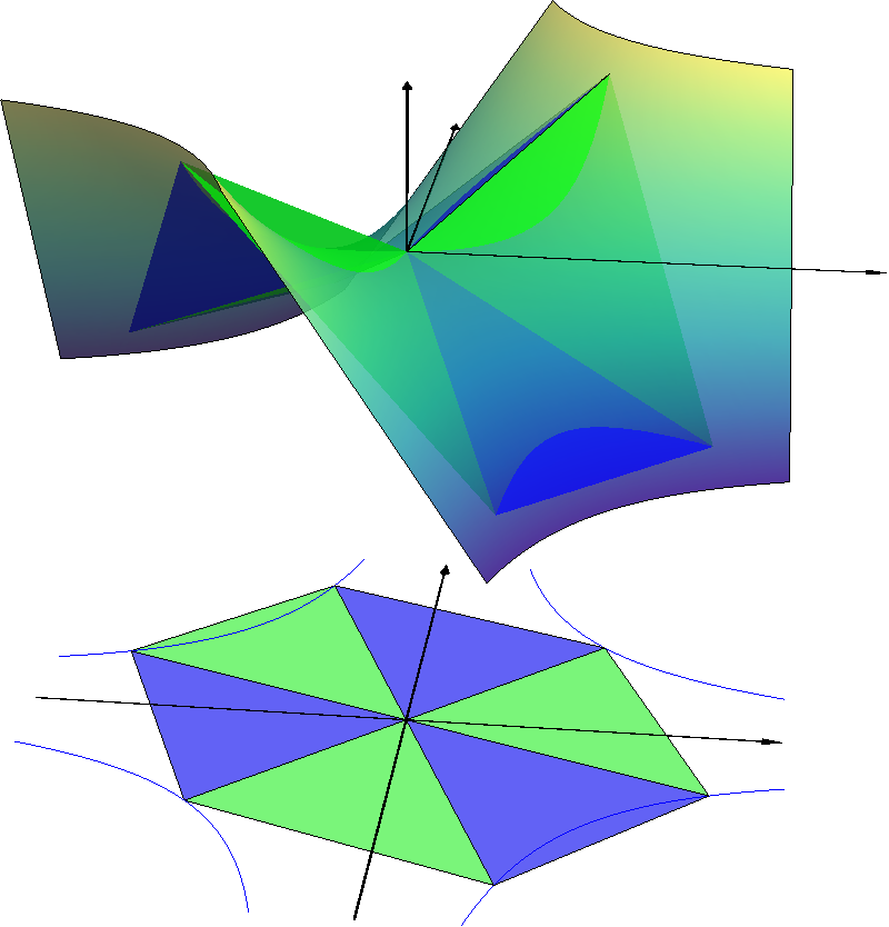
(a)	(b)

Figure 7: The triangles surrounding the origin in an optimal interpolating triangulation of a saddle surface. Depending on the chosen orientation, the approximating triangulation will predominantly lie (a) above the surface or (b) below the surface.

Incidentally, the same fallacious line of reasoning has led L. Fejes Tóth, in his celebrated book Lagerungen in der Ebene, auf der Kugel und im Raum from 1953 (Fejes Tóth, 1972, Section V.12, p. 151), to assert erroneously that a ruled surface such as a hyperboloid of one sheet could be triangulated with a triangle density of only $O(1/\sqrt{\varepsilon})$. For more details, see Wintraecken (2015, Section 2.4).

3.2 Non-interpolating approximation

In this section, we will prove our main result, Theorem 1.1, which concerns non-interpolating approximation. When we try to improve the approximation by allowing the vertices of the triangles to move away from the surface, we encounter a challenge: In contrast to the convex case, some edges (the ascending ones) run above $f$ and others (the descending ones) run below $f$. Figure 7 shows that the linear approximation penetrates the surface $f$, lying partially above it and below it. It is not clear in which direction one should start moving the vertices to improve the approximation. Accordingly, Pottmann, Krasauskas, Hamann, Joy, and Seibold (2000) conjectured that the best approximation is the interpolating approximation. We will see that this is not the case.

To make the problem manageable, we impose the following constraint: Every vertex of the approximations has the same offset $\Delta$ (positive or negative) from the surface. This ensures that we can apply Lemma 2, and it suffices to look for one triangle that maximizes the area.

Lemma 4 must be modified to take into account the vertical shift by $\Delta$.

Lemma 6

Let $p,q\in\mathbf{R}^{2}$ be two points. The maximum vertical error between $f$ and the linear interpolation between $f(p)+\Delta$ and $f(q)+\Delta$ is attained either at the midpoint $(p+q)/2$ or at the endpoints $p$ and $q$, and its value is

$$\max_{0\leq\lambda\leq 1}|(1-\lambda)f(p)+\lambda f(q)+\Delta-f((1-\lambda)p+\lambda q)|=\max\{|\Delta|,|\Delta+\tfrac{f(q-p)}{4}|\}.$$ ∎

Let us fix a point $p_{1}$ and ask for the possible locations of a point $p_{2}$ such that the approximation error on the edge $p_{1}p_{2}$ does not exceed $\varepsilon$. Assuming that $|\Delta|\leq\varepsilon$, we can rewrite the condition $|\Delta+{f(q-p)}/4|\leq\varepsilon$, and we see that the vector $(x,y)=(x_{2}-x_{1},y_{2}-y_{1})$ must satisfy the inequalities

$$-(\varepsilon+\Delta)\leq xy/2\leq\varepsilon-\Delta.$$

This is a region bounded by two different hyperbolas, see Figure 5b, but the arguments from the previous section about the concavity of the region remain valid, showing that the error must be attained at all three edges (Lemma 5). As before, we can also assume that $p_{1}$ lies at the origin and $p_{2}$ and $p_{3}$ lie in the first quadrant. (To achieve the last situation, we may have to switch the sign of $\Delta$.) In this situation, $f(x_{2},y_{2})$ and $f(x_{3},y_{3})$ are positive, and we have $x_{2}y_{2}=x_{3}y_{3}=2(\varepsilon-\Delta)$. Again, by a pseudo-Euclidean transformation, we simplify the computation by assuming the symmetric situation $(x_{3},y_{3})=(y_{2},x_{2})$. The third edge $p_{2}p_{3}$ is descending, because it is a chord of the hyperbola in the first quadrant. Thus, with $p_{3}-p_{2}=(x_{3}-x_{2},y_{3}-y_{2})$, the quadratic function $f(p_{3}-p_{2})$ will be negative, and we get the equation $f(p_{3}-p_{2})=-4(\varepsilon+\Delta)$. The term $f(p_{3}-p_{2})$ evaluates to $f(p_{3}-p_{2})=-2(y_{2}-x_{2})^{2}=-2(2(\varepsilon-\Delta)/x_{2}-x_{2})^{2}$. Solving the resulting quadratic equation

$$x_{2}^{2}\pm\sqrt{2(\varepsilon+\Delta)}x_{2}-2(\varepsilon-\Delta)=0$$

gives

$$p_{2}=(x_{2},y_{2})=\Bigl{(}\sqrt{\tfrac{1}{2}}\cdot(\sqrt{5\varepsilon-3\Delta}\pm\sqrt{\varepsilon+\Delta}),\,\sqrt{\tfrac{1}{2}}\cdot(\sqrt{5\varepsilon-3\Delta}\mp\sqrt{\varepsilon+\Delta})\Bigr{)}.$$

As in (5), the area of a symmetric triangle $(0,0)$, ($x_{2},y_{2})$, ($y_{2},x_{2})$ is $\tfrac{1}{2}|(x_{2}+y_{2})(x_{2}-y_{2})|$. This evaluates to $\sqrt{5\varepsilon-3\Delta}\cdot\sqrt{\varepsilon+\Delta}=\sqrt{3}\cdot\sqrt{5\varepsilon/3-\Delta}\cdot\sqrt{\varepsilon+\Delta}$, and this is maximized for $\Delta=\varepsilon/3$, yielding an area of $4/\sqrt{3}\cdot\varepsilon$. The necessary condition $|\Delta|\leq\varepsilon$ is fulfilled. By Lemma 2, this establishes Theorem 1.1. ∎

Figure 8: Optimal non-interpolating triangles, together with the hyperbolas $|xy|=2\varepsilon$.

Figure 8 shows six reflected copies of the optimal triangle surrounding the origin, together with the hyperbolas $xy=\pm 2\varepsilon$ that were used to define the optimal interpolating triangulation. The optimal triangle turns out to be an equilateral triangle (of side length $\sqrt{8\varepsilon/3}$), and it happens to touch the hyperbola $xy=2\varepsilon$. We do not have an explanation for these phenomena.

Pottmann et al. (2000) proposed to call the optimal triangles for the interpolating approximation of the function $xy$, as defined in Section 3.1, the equilateral triangles of pseudo-Euclidean geometry. Maybe it would be more appropriate to reserve this name for the triangles of Figure 8 and their pseudo-Euclidean transformations, in view of their remarkable properties.

4 Concluding remarks

The constants in Theorems 1.1 and 1.2 are very close. Thus, the freedom to use non-interpolating approximations seems to give only a slight improvement. This is in contrast to the case of convex functions (Theorem 1.3), where non-interpolating approximations are better by a factor of 2.

The optimality of the approximations found in Theorem 1.1 remains open. If different vertices have different offsets, one is forced to use more than just one type of triangle, and the situation becomes complicated.

In contrast to this, we know that the constants in Theorems 1.2 and 1.3 about non-convex interpolating approximation and about convex interpolations are best possible. The expressions of Theorems 1.2 and 1.3 hold therefore as lower bounds on the triangle density of any triangulation. This follows from the proofs, because a triangulation of density $D$ must contain triangles of area at least $1/D-\delta$ for arbitrarily small $\delta>0$. These lower bounds also apply when we want to triangulate a bounded polygonal domain $\Omega$. The triangle density is then simply the number of triangles divided by the area of $\Omega$. In this case, the bound cannot be achieved in general, because the grid has to adapt to the boundary of $\Omega$, but it can be attained asymptotically as $\varepsilon\to 0$.

Another question that would be worth while to be attacked would be good (or optimal) triangulations for trivariate quadratic functions.

References

- Atariah [2014] Dror Atariah. Parameterizations in the Configuration Space and Approximations of Related Surfaces. PhD thesis, Freie Universität Berlin, 2014. www.diss.fu-berlin.de/diss/receive/FUDISS_thesis_000000096803.
- Atariah et al. [2013] Dror Atariah, Sunayana Ghosh, and Günter Rote. On the parameterization and the geometry of the configuration space of a single planar robot. Journal of WSCG, 21:11–20, 2013.
- Bertram et al. [2000] Martin Bertram, James C. Barnes, Bernd Hamann, Kenneth I. Joy, Helmut Pottmann, and Dilinur Wushour. Piecewise optimal triangulation for the approximation of scattered data in the plane. Computer Aided Geometric Design, 17(8):767–787, 2000. doi:10.1016/S0167-8396(00)00026-1.
- Clarkson [2006] Kenneth L. Clarkson. Building triangulations using -nets. In Proceedings of the 38th Annual ACM Symposium on Theory of Computing, STOC’06, pages 326–335. ACM Press, 2006. ISBN 1-59593-134-1. doi:10.1145/1132516.1132564.
- Fejes Tóth [1972] László Fejes Tóth. Lagerungen in der Ebene, auf der Kugel und im Raum, volume 65 of Die Grundlehren der mathematischen Wissenschaften. Springer-Verlag, 2nd edition, 1972.
- Pottmann et al. [2000] Helmut Pottmann, Rimvydas Krasauskas, Bernd Hamann, Kenneth Joy, and Wolfgang Seibold. On piecewise linear approximation of quadratic functions. Journal for Geometry and Graphics, 4(1):9–31, 2000.
- Wintraecken [2015] Mathijs H. M. J. Wintraecken. Ambient and Intrinsic Triangulations and Topological Methods in Cosmology. PhD thesis, Rijksuniversiteit Groningen, 2015.