Edge-state blockade of transport in quantum dot arrays

Abstract

We propose a transport blockade mechanism in quantum dot arrays and conducting molecules based on an interplay of Coulomb repulsion and the formation of edge states. As a model we employ a dimer chain that exhibits a topological phase transition. The connection to a strongly biased electron source and drain enables transport. We show that the related emergence of edge states is manifest in the shot noise properties as it is accompanied by a crossover from bunched electron transport to a Poissonian process. For both regions we develop a scenario that can be captured by a rate equation. The resulting analytical expressions for the Fano factor agree well with the numerical solution of a full quantum master equation.

I Introduction

Quantum electronics is governed by charging energies which give rise to Coulomb blockade which is apparent in the diamond-like charging diagrams of quantum dots van der Wiel et al. (2003) and conducting molecules Cuevas and Scheer (2010). When electron spins and phonons come into play, additional blockade phenomena may influence the current-voltage characteristics. For example, the Pauli exclusion principle may cause a spin blockade in double Weinmann et al. (1995); Ono et al. (2002) and triple quantum dots Busl et al. (2013). Moreover, in suspended quantum dots, an entering electron may emit a phonon and become trapped until it reabsorbs a phonon, which is known as a phonon blockade Weig et al. (2004).

Some blockade phenomena are less pronounced in the current, but have a strong impact on the current noise. Most prominently, the strong coupling of an electron in a molecular wire with a vibrational degree of freedom may lead to a switching between conducting and almost isolating configurations and cause Franck-Condon blockade. Then the transport becomes avalanchelike, which drastically enhances the shot noise Koch and von Oppen (2005); Leturcq et al. (2009). A similar effect occurs in capacitively coupled transport channels, where noise measurements reveal that a mutual channel blockade causes electron bunching Barthold et al. (2006); Sánchez et al. (2008).

A one-dimensional tight-binding model with alternating tunnel matrix elements represents a simple description of a dimerized polymer Su et al. (1979). It is characterized by a topological invariant, the Zak phase Zak (1989), which depends on the ratio between the inter- and intradimer coupling and has been measured recently Atala et al. (2013). For finite chains in the topologically nontrivial phase, a pair of exponentially decaying edge states emerges Delplace et al. (2011). Moreover, Coulomb interaction may lead to long-range tunneling of doublons between edge states Bello et al. (2016). When the chain is in contact with the electron source and drain, however, the impact of the edge states on the transport properties remains an open question.

In this paper we propose an edge-state current blockade in voltage-biased arrays such as that sketched in Fig. 1, which relates to the transition from a topologically trivial to a nontrivial regime. We show that it is most clearly visible in the shot noise. In Sec. II, we introduce our model and a master equation description. The main results and the physical mechanism of the resulting transport are presented in Sec. III. Finally, in Sec. IV we discuss possible experimental realizations and draw our conclusions in Sec. V. Some technical aspects of the numerical scheme and details of the calculations can be found in the Appendixes.

II Model and master equation

We employ spinless electrons on an array of length $N$ described by the Hamiltonian $H_{0}=H_{\text{SSH}}+H_{\text{int}}$. It contains nearest-neighbor tunneling according to the Su-Shrieffer-Heeger (SSH) Hamiltonian Su et al. (1979)

$$H_{\text{SSH}}=\sum_{n=1}^{N-1}\tau_{n}c_{n+1}^{\dagger}c_{n}+\text{H.c.},$$ (1)

with the alternating tunnel matrix elements $\tau_{n}=\tau_{0}+(-1)^{n}\delta\tau$ and the fermionic annihilation operator $c_{n}$. We keep $\tau_{0}$ constant and use $\delta\tau$ as a control parameter.

The SSH model is probably the simplest one with a topological phase transition. For $\delta\tau<0$, it describes a chain of weakly coupled dimers which form two bands with a gap that closes at $\delta\tau=0$. When $\delta\tau$ assumes positive values, two edge states emerge [see the inset of Fig. 2(a)]. In the bulk, the wave function of the edge states decays exponentially with a localization length given by the inverse of $\kappa=\ln(\tau/\tau^{\prime})\approx 2\delta\tau/\tau_{0}$. Thus, for finite arrays, the edge states form a doublet with a level splitting $\Delta\approx\tau_{0}\exp({-N\delta\tau/\tau_{0}})$ (see Appendix A). It will turn out that this doublet governs the transport properties for $\delta\tau>0$. If the array consists of an odd number of sites, a monomer will remain forming an edge state. Thus, we witness a transition from a situation with an edge state at the right end of the chain ($\delta\tau<0$) to one with an edge state at the left end ($\delta\tau>0$) Bernevig (2013). This transition, however, is not visible in the spectrum [see inset of Fig. 2(b)].

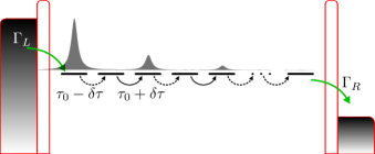
Figure 1: Dimer chain with tunnel couplings $\tau^{\prime}=\tau_{0}-\delta\tau$ and $\tau=\tau_{0}+\delta\tau$, respectively, connected to the electron source (left) and drain (right). At $\delta\tau=0$, the chain undergoes a topological phase transition. The wave function depicts the stationary state in the topological regime. Electron trapping in the edge state at the source causes an edge-state blockade.

For the Coulomb repulsion, we assume $H_{\text{int}}=\sum_{n>n^{\prime}}U_{|n-n^{\prime}|}N_{n}N_{n^{\prime}}$ with the site occupations $N_{n}$ and the interaction energies $U_{d}$ which decay with the distance $d=n-n^{\prime}$ between the sites. Moreover, by working with spinless electrons, we have already ruled out double occupation of a single site. Physically, this is justified by the typically very strong on-site interaction $U_{0}$ in quantum dots.

To enable transport, we couple the ends of the array to biased leads acting as the electron source and drain with a voltage bias $V$. Within second-order order perturbation theory we integrate out the leads to obtain a Bloch-Redfield type master equation for the reduced density operator. For low temperatures and in the limit $\tau,\tau^{\prime}\ll eV\ll U_{d}<U_{0}$, only single-electron states are energetically accessible and the electron transport becomes unidirectional. Moreover, the array-lead tunneling becomes independent of the details of the array’s level structure. Then the master equation assumes the convenient Lindblad form

$$\dot{\rho}=\mathcal{L}\rho\equiv-\frac{i}{\hbar}[H_{\text{SSH}},\rho]+\Gamma_{L}\mathcal{D}(c_{1}^{\dagger})\rho+\Gamma_{R}\mathcal{D}(c_{N})\rho,$$ (2)

with $\mathcal{D}(x)\rho=(2x\rho x^{\dagger}-x^{\dagger}x\rho-\rho x^{\dagger}x)/2$ and the dot-lead rates $\Gamma_{L,R}$. The first term in $\mathcal{D}(x)$ corresponds to incoherent transitions induced by the operator $x=c_{1}^{\dagger},c_{N}$, which in our case is the electron tunneling from the source to the array and from the array to the drain, respectively. Thus, the (particle) current is described by the superoperator $\mathcal{J}\rho=\Gamma_{L}c_{1}^{\dagger}\rho c_{1}$ (or alternatively by $\Gamma_{R}c_{N}\rho c_{N}^{\dagger}$). Notice that neither the bias $V$ nor the interaction constant $U$ appear explicitly in Eq. (2). Let us therefore emphasize that our master equation holds only in the limit in which strong Coulomb repulsion inhibits the occupation with two or more electrons, i.e., it has to be evaluated in the subspace of zero or one electrons on the chain. As a consequence, the dynamics on the chain is governed by the single-particle quantum mechanics induced by the SSH Hamiltonian, while the electron tunneling from the source to the chain is affected by the interaction.

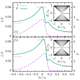
Figure 2: Current (dashed line) and Fano factor $F=C_{2}/|I|$ (solid line) for an array of (a) $N=20$ and (b) $N=21$ sites as a function of the imbalance $\delta\tau/\tau_{0}$ and the lead couplings $\Gamma_{R}=\Gamma_{L}=5\tau_{0}$. The dotted horizontal lines mark the analytically obtained limits. Despite the different single-particle spectra (insets), the results for an even and odd number of sites are qualitatively the same.

Low-frequency current fluctuations can be characterized by the counting statistics of the transported electrons. For this purpose, we introduce a counting variable $\chi$ and consider the modified master equation $\dot{R}_{\chi}=\mathcal{L}_{\chi}R_{\chi}$ with $\mathcal{L}_{\chi}=\mathcal{L}+(e^{i\chi}-1)\mathcal{J}$ Bagrets and Yu. V. Nazarov (2003); Novotný et al. (2004). It is constructed such that $\mathop{\mathrm{tr}}\nolimits(R_{\chi})=\langle e^{i\chi N_{R}}\rangle$ becomes the moment generating function for the electron number in the drain, $\phi(\chi,t)$. The current cumulants $C_{n}=(\partial/\partial{i\chi})^{n}\ln\dot{\phi}(\chi,t)|_{\chi=0,t\rightarrow\infty}$ contain the full information about the low-frequency noise. The spectral decomposition of $R_{\chi}$ into the eigenbasis of $\mathcal{L}_{\chi}$ yields a formal solution which at long times is dominated by the eigenvalue with the largest real part, $\lambda_{0}(\chi)$. Then, $R_{\chi}\propto\exp[\lambda_{0}(\chi)t]$ and, thus, $\ln\phi(\chi,t)=\lambda_{0}(\chi)t$. Being interested in derivatives close to $\chi=0$, we can treat $\chi$ as a small parameter and obtain the cumulants from an iteration based on the Rayleigh-Schrödinger perturbation theory Flindt et al. (2008). The first two steps yield the current $I=C_{1}=\mathop{\mathrm{tr}}\nolimits(\mathcal{J}\rho_{0})$ and the variance $C_{2}=I-2\mathop{\mathrm{tr}}\nolimits(\mathcal{J}\mathcal{R}\mathcal{J}\rho_{0})$ Novotný et al. (2004), where $\rho_{0}$ is the stationary solution of the master equation (2) and $\mathcal{R}$ is the pseudo inverse of $\mathcal{L}$. For details, see Appendix B.

It is worthwhile to define the Fano factor $F=C_{2}/|I|$, which is a dimensionless measure of the noise strength and hints at the nature of the transport mechanism Ya. M. Blanter and Büttiker (2000). The value $F=1$ corresponds to uncorrelated events, while larger values indicate bunching. For more profound statements, one has to consider also cumulants of higher order.

III Edge states, current, and shot noise

III.1 General scenario for dimer chains

Let us start by investigating a dimer chain, i.e., the case of an even number of sites for which the current in the different regimes is shown in Fig. 2(a). We notice that in the monomer limit $\delta\tau=0$, the current assumes an appreciable value. Towards both the topologically trivial and the nontrivial region, it decays. In the nontrivial region, the decay is faster despite the presence of interband states. The asymmetry is also found for the Fano factor which is super-Poissonian for $\delta\tau\lesssim 0$, while for $\delta\tau>0$ it converges to the Poissonian value $F=1$. This indicates that the transport relates to topology.

To reveal the physics behind this observation, we conjecture for each region a dominating mechanism and capture it by a rate equation that provides analytical expressions for the current and the Fano factor. For the monomer chain realized at the transition point $\delta\tau=0$ (for finite systems it is rather a crossover at $\delta\tau\approx\tau_{0}/N$ Delplace et al. (2011)), the eigenstates read $\phi_{\ell}(n)\propto\sin[\pi\ell n/(N+1)]$, where $\ell=1,\ldots,N$, labels the solutions. We assume that each eigenstate forms a transport channel, where a strong Coulomb interaction leads to mutual exclusion of the channel occupation. The corresponding load and unload rates $\gamma_{\ell}^{L,R}$ are determined by the overlaps with the terminating sites, i.e., by $|\phi_{\ell}(1)|^{2}$ and $|\phi_{\ell}(N)|^{2}$. For a symmetric setup, $\gamma_{\ell}^{L}=\gamma_{\ell}^{R}\equiv\gamma_{\ell}$. States with $\ell\approx N/2$ are much stronger coupled to the leads than those with $\ell=1$ or $\ell=N$ and, thus, most of the time, the strongly coupled states support a regular current. However, whenever a weakly coupled state becomes populated, an electron will remain there for the rather long time $\gamma_{\ell}^{-1}$ and thereby interrupt the transport process. Accordingly, we expect bunching as is indicated by a large Fano factor. For a quantitative treatment, we formulate the above scenario as a rate equation from which we obtain the current $I=\Gamma/(N+1)$ and the Fano factor $F_{\text{mono}}(N)\approx(N-2)/3$. Since the effects are most noticeable in longer arrays, we ignore corrections of the order $N^{-1}$. For the full expressions and their derivation, see Appendix C.1.

Deep in the trivial region $\delta\tau<0$, the central system consists of weakly coupled dimers. Then we can consider each dimer as one site and, thus, expect the behavior of a monomer array with $N/2$ sites. Therefore, without an explicit calculation, we can conclude that the Fano factor is $F=F_{\text{mono}}(N/2)$.

Finally, in the topological region $\delta\tau>0$, the electrons mainly enter and leave the array via an edge state which is at zero energy. Since all other states are energetically far off, they merely mediate long-range tunneling with the exponentially small effective matrix element $\Delta$ given above. This means that the situation can be captured by a two-level system. For a sufficiently large array, $\Delta\ll\Gamma$, the bottleneck of the transport is the tunneling between edge states. The corresponding current reads $I\simeq\Delta^{2}/\Gamma$ and consists of uncorrelated events Kaiser et al. (2006), i.e., it is a Poissonian process with the characteristic Fano factor $F=1$. For an explicit derivation, see Appendix C.2.

The Fano factor of the full numerical calculation agrees rather well with the limits obtained analytically [see the horizontal lines in Fig. 2(a)]. This provides evidence that the transport process in each region indeed follows the scenario sketched above.

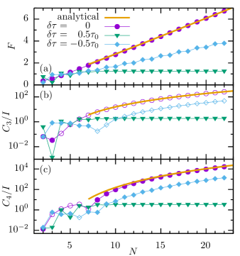
Figure 3: (a) Fano factor, (b) third cumulant and (c) fourth cumulant as a function of the chain length for various $\delta\tau$ and the lead coupling $\Gamma_{R}=\Gamma_{L}=5\tau_{0}$. Solid symbols mark positive values and stroked symbols correspond to negative values.

Since the separation of the Fano factors in the different regions grows with the length of the array, one may aim at an experimental realization with as many sites as possible. This, however, will raise the experimental difficulties drastically. Moreover, beyond a certain system size, the limit of a strong Coulomb blockade may no longer be realistic. Thus the length dependence of the Fano factors deserves a closer inspection. The data shown in Fig. 3(a) confirm our analytical results even down to rather small lengths. For an intermediate length $N\approx 10$, the Fano factors in the three regimes are already significantly different from each other. In particular, the differences are larger than the demonstrated resolution of mesoscopic noise measurements Kießlich et al. (2007). The data for cumulants of higher order presented in Figs. 3(b) and 3(c) support our conjecture of Poissonian transport in the topological phase.

III.2 Arrays with an odd number of sites

A further important observation is that the behavior of the shot noise for chains with an odd number of sites interpolates the behavior of dimer chains. In particular, we find that the current and the Fano factor as a function of $\delta\tau$ indeed are qualitatively the same as for even $N$ [see Fig. 2(b)].

For odd $N$, irrespective of the sign of $\delta\tau$, there always exists one edge state which has zero energy [see the spectrum shown in the inset of Fig. 2(b)]. Thus, the chain does not exhibit a transition between a topological and a nontopological phase. Nevertheless, the emergence of the edge state at one specific end of the chain can be explained in terms of the bulk-edge correspondence as follows. Let us consider a not too short chain with even $N$ and $\delta\tau>0$, such that the tunnel splitting $\Delta\sim\exp(-N\delta\tau/\tau_{0})$ between the edge states is much smaller than the lead coupling $\Gamma$. Then decoherence will turn a possible superposition of both edge states into a mixture so that the edge state at the source will not be influenced by its counterpart at the drain. Then removing the last site of the chain will not have a major effect on the edge-state formation at the source. In this sense, also finite chains with odd $N$ still exhibit some footprint of a topological transition that is found for infinite or semi-infinite dimer chains.

The common feature for even and for odd $N$ is that only for $\delta\tau>0$, does the chain possess an edge state at the electron source. The relevance of its location at the source is visible in the behavior under inverting the applied bias: For even $N$, the chain is symmetric, so that only the direction of the current changes. Therefore, the Fano factor in Fig. 2(a) will remain the same. For odd $N$, by contrast, the inverted bias leads to a situation with an edge state at the drain but none at the source. Thus, bias inversion is equivalent to changing the sign of $\delta\tau$, which for odd $N$ moves the edge state from one end of the chain to the other. Therefore, upon bias inversion, $F$ in Fig. 2(b) becomes reflected at the $y$ axis (not shown).

III.3 Blocking mechanism and localization

To underline the importance of the edge state and to develop a physical picture for the blockade, we consider the population of the sites in the stationary state of the open system [see Fig. 4]. For an even number of sites [Figs. 4 (a) and 4(b), where the latter is computed with source and drain interchanged], in the topological phase ($\delta\tau>0$) the edge state at the source is predominantly populated. This is consistent with the scenario drawn above in which the transport occurs via weak long-range tunneling. Consequently, an electron becomes trapped in the edge state localized at the source, while once it is at the opposite side of the array, it leaves quickly to the drain.

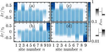
Figure 4: Population of the quantum dots in the stationary state for the array lengths (a),(b) $N=10$ and (c),(d) $N=9$ and the lead coupling $\Gamma_{R}=\Gamma_{L}=5\tau_{0}$. The data in the lower row are with the source and drain interchanged, as indicated by the sketches at the right margin. They reveal that a current blockade emerges when the edge state at the source is strongly populated (dark blue areas). Comparing the upper row with the lower row highlights the reflection symmetry for even $N$, while for odd $N$ the spatial reflection corresponds to inverting the sign of $\delta\tau$.

For an odd number of sites, the behavior is similar. Outside the crossover region $|\delta\tau|\gg\tau_{0}$, one edge state always exists. For $\delta\tau>0$, it is localized at site $1$ and causes a current blockade [see Fig. 2(b)]. By contrast, for $\delta\tau<0$, despite the emergence of an edge state at site $N$, an appreciable current flows.

To resolve this seeming contradiction, let us focus on an array with odd $N$ and $\delta\tau<0$ such that an edge state at the drain is formed. Nevertheless, a small overlap of the bulk states with the last site opens a way to circumvent the edge state. Moreover, in rare cases in which an electron reaches the edge state, it will proceed quickly to the drain, consequently, no relevant blockade occurs. For $\delta\tau>0$, the edge state is located at the source and is mostly occupied [see Fig. 4(c)]. Then, bypassing site 1 is in principle possible, but would require double occupation of the chain. This, however, is inhibited by Coulomb repulsion so that transport is interrupted until the electron in the edge state is released. This reveals that the blockade results from an interplay of edge-state formation at the source and strong Coulomb repulsion. The population for interchanged source and drain [Fig. 4(d)] confirms that the edge-state formation at the source is also decisive for trapping an electron when $N$ is odd.

III.4 Disorder

The formation of edge states with exponentially small splitting is protected by sublattice symmetry present in our idealized array Hamiltonian $H_{\text{SSH}}$. In a realistic experiment, however, it may be quite difficult to tune the system sufficiently well. To investigate the influence of imperfections, we consider disorder and add random on-site energies,

$$H_{\text{SSH}}\to H_{\text{SSH}}+W\sum\xi_{n}c_{n}^{\dagger}c_{n},$$ (3)

where $W$ is the disorder strength and $\xi_{n}$ is taken from a normalized box distribution with $-1/2\leq\xi_{n}\leq 1/2$.

Figure 5 shows the resulting Fano factor, now defined as $\bar{C}_{2}/\bar{I}$, i.e., the ratio of the averages. Comparing Figs. 5(a) and 5(b), the behavior for an even and an odd number of sites again turns out to be practically the same. For $\delta\tau\lesssim 0$, we find that the Fano factor grows with increasing disorder. The enhancement is roughly $\propto W^{2}$, as can be appreciated in the inset. Notice that for larger values of $W$ and much longer arrays, Anderson localization Anderson (1958) becomes relevant and may change this behavior.

For $\delta\tau>0$, by contrast, disorder has almost no influence on the Fano factor. This finding is consistent with the physical picture drawn above: The transport occurs via the two states localized at the ends of the array, while the other states are off-resonant and not populated. Since disorder even supports localization, the Poissonian behavior remains unaffected.

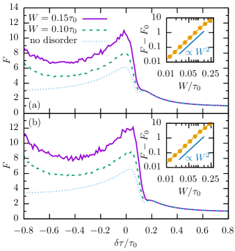
Figure 5: Fano factor in the presence of disorder with strength $W$ for a chain of lengths (a) $N=20$ and (b) $N=21$ with the parameters used in Fig. 2. Insets: Deviation of the averaged Fano factor from its value in the absence of disorder for $\delta\tau=-0.5\tau_{0}$.

IV Possible experimental realization

The high tunability of the various types of quantum dots makes them natural candidates for the implementation of blockade effects in mesoscopic transport. Recently, two parallel quantum dot arrays, each with seven dots, have been demonstrated Puddy et al. (2015). In such systems, the charging and the tunnel matrix elements are highly controllable by gate voltages. Thus it should be possible to tune them such that they meet the requirement of an interaction much larger than the tunneling, at least in not too long arrays.

Molecular wires represent a realistic alternative, in particular, since they are rather small and thus possess huge charging energies. Between experimental runs, they can be modified by atomic force microscopy techniques Kocić et al. (2015). Since this may also affect wire-lead tunneling rates, the visibility of the blockade in the Fano factor is a virtue since this quantity, in contrast to the current, depends only weakly on the wire-lead coupling. Moreover, one may change the topology of the molecule by ac fields Gómez-León and Platero (2013).

V Conclusions

We have investigated a current blockade mechanism for strongly biased contacted dimer chains. It results from an interplay of Coulomb repulsion and edge-state formation which relates to a topological transition. The edge state at the source can trap an electron, while Coulomb repulsion inhibits a further electron to enter the chain. The resulting electron transport consists of rare tunnel events between the edge states and exhibits a characteristic Poissonian behavior. By contrast, in the topologically trivial region, we find transport through delocalized states and electron bunching. Since the edge state at the source turned out to be responsible, the effect can be observed also in chains with an odd number of sites in which a different but related transition occurs, namely, the displacement of the edge state from one end to the other. Clear experimental evidence for the transition between the different regions can be provided by shot noise measurements. While we have demonstrated that the mechanisms on both sides of the transition are fairly insensitive to static disorder, a more realistic description of an implementation with molecular wires should consider also spin effects, vibrational degrees of freedom, and decoherence.

Appendix A Overlap of the edge states

The Schrödinger equation for a dimer chain with intra- and interdimer couplings $\tau$ and $\tau^{\prime}$, respectively, is

$$\tau\sigma_{+}\phi_{n-1}+\tau^{\prime}\sigma_{x}\phi_{n}+\tau\sigma_{-}\phi_{n+1}=\epsilon_{n}\phi_{n},$$ (4)

where $\phi_{n}=\left(c_{2n},c_{2n+1}\right)^{T}$ and $n$ labels the unit cells. For periodic boundary conditions we use the Bloch ansatz $\phi_{n}=e^{ikn}\varphi(k)$ and obtain the Bloch equation

$$\begin{pmatrix}0&\tau e^{-ik}+\tau^{\prime}\\ \tau e^{ik}+\tau^{\prime}&0\end{pmatrix}\varphi(k)=\epsilon(k)\varphi(k).$$ (5)

An edge state in a semi-infinite chain corresponds to a solution that vanishes at some site such that, e.g., $\phi_{-1}=0$. Then, we obtain from the Schrödinger equation and Eq. (5) the condition

$$\begin{pmatrix}0&\tau^{\prime}\\ \tau e^{ik}+\tau^{\prime}&0\end{pmatrix}\varphi(k)=0.$$ (6)

It possesses a nontrivial solution if $k=\pi+i\ln(\tau/\tau^{\prime})$, which for $\tau>\tau^{\prime}$ is decaying as $\phi_{n}\propto\exp(-\kappa n)$ with the exponent $\kappa=\ln(\tau/\tau^{\prime})$. Close to the phase transition $|\delta\tau|\ll\tau_{0}$, it becomes $\kappa=2\delta\tau/\tau_{0}$. Therefore, the overlap between the two edge states of a chain with $N/2$ dimers can be estimated as

$$\Delta\approx\tau_{0}e^{-\delta\tau N/\tau_{0}}.$$ (7)

It agrees with the splitting of the interband doublet found in finite dimer chains Delplace et al. (2011).

Appendix B Iteration scheme for the cumulants

As we are interested in the statistics of the transport, we need to generalize the master equation formalism, introducing a counting variable $\chi$ which keeps track of the electron number in the leads. The cumulants of the corresponding distribution function are given by the $k$th derivatives with respect to $i\chi$ at $\chi=0$ of the logarithm of the moment generating function $\phi(\chi,t)=\langle e^{i\chi N_{R}}\rangle$. The moment generating function can be written as the trace of the generalized reduced density operator $R_{\chi}(t)=\mathop{\mathrm{tr}}\nolimits_{\text{leads}}(\rho_{\text{tot}}e^{i\chi N_{R}})$, which obeys the master equation

$$\dot{R}_{\chi}(t)=\mathcal{L}_{\chi}R_{\chi}(t),$$ (8)

where $\mathcal{L}_{\chi}=\mathcal{L}+\left(e^{i\chi}-1\right)\mathcal{J}$. Notice that we have restricted ourselves to unidirectional transport, i.e., to the limit of large bias in which all relevant eigenstates of the conductor are within the voltage window and thermal excitations do not play a role.

In the long-time limit, the dynamics of $R_{\chi}(t)$ is governed by the eigenvalue of $\mathcal{L}_{\chi}$ with the largest real part, denoted as $\lambda_{0}(\chi)$. Then, $R_{\chi}(t)\propto\exp[\lambda_{0}(\chi)t]$ and, thus, $\ln\phi(\chi,t)=\lambda_{0}(\chi)t$ (besides a correction that vanishes in the long-time limit). Instead of calculating the proper eigenvalue of $\mathcal{L}_{\chi}$ and its derivatives with respect to $\chi$, one can treat $\chi$ as a small parameter and obtain the cumulants from an iteration based on Rayleigh-Schrödinger perturbation theory Flindt et al. (2008); Domínguez et al. (2010). The solution in the Markovian case is

$$C_{k}=\sum_{k^{\prime}=0}^{k-1}\binom{k}{k^{\prime}}\mathop{\mathrm{tr}}\nolimits(\mathcal{J}P_{k^{\prime}}),$$ (9)

where $C_{0}=0$ and $\mathcal{L}P_{0}=0$. The other components $P_{k}$ follow from the equation

$$\mathcal{L}P_{k}=-\sum_{k^{\prime}=0}^{k-1}\binom{k}{k^{\prime}}(\mathcal{J}-C_{k-k^{\prime}})P_{k^{\prime}}\,,$$ (10)

which has to be solved under the condition $\mathop{\mathrm{tr}}\nolimits P_{k}=0$. This step is equivalent to applying the pseudoinverse of the Liouvillian to the right-hand side of Eq. (10). In this way, the first cumulant, i.e., the current, can be written as $C_{1}=\mathop{\mathrm{tr}}\nolimits(\mathcal{J}P_{0})$. This enables the computation of $P_{1}$ from the equation $\mathcal{L}P_{1}=-(\mathcal{J}-C_{1})P_{0}$. Then the second cumulant, i.e., the zero-frequency noise, becomes $C_{2}=C_{1}+2\mathop{\mathrm{tr}}\nolimits(\mathcal{J}P_{1})$.

Appendix C Analytical approach to the transport cumulants

The current for the full model follows directly from the stationary solution of the master equation (2) of the main text, i.e., from the kernel of the Liouvillian $\mathcal{L}$. It can be computed analytically, which allows us to evaluate the expression for the current. For an even number of sites, we obtain

$$I_{\text{even}}=\frac{\Gamma_{R}}{N+\frac{\Gamma_{R}}{\Gamma_{L}}+\frac{\Gamma_{R}^{2}}{4\tau^{2}}\left[N-2+\left(\frac{\tau}{\tau^{\prime}}\right)^{N}\right]},$$ (11)

while for odd $N$, the current reads

$$I_{\text{odd}}=\frac{\Gamma_{R}}{\frac{\Gamma_{R}}{\Gamma_{L}}+\frac{\Gamma_{R}^{2}\left(N-1\right)}{4\tau^{2}}+\left(\frac{\tau^{\prime}}{\tau}\right)^{2}\left[N-1+\left(\frac{\tau}{\tau^{\prime}}\right)^{N+1}\right]}.$$ (12)

Both expressions assume their maximum close to $\tau\approx\tau^{\prime}$. For $\tau\gg\tau^{\prime}$, i.e., in the region in which we find edge-state blockade, it decays $\propto(\tau^{\prime}/\tau)^{N}$. In the opposite limit, $\tau\ll\tau^{\prime}$, the decay is algebraic, $I\propto N^{-1}$ (see Fig. 6).

By contrast, computing the cumulants $C_{n}$ with $n\geq 2$ requires not only the kernel of the Liouvillian, but also its pseudoinverse, which considerably complicates the analytical solution. To nevertheless find analytical results for the noise, below we develop a description with a simplified master equation for the two limits discussed in the main text.

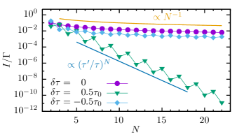
Figure 6: Stationary current as a function of the chain length for the values of $\delta\tau$ displayed. The dot-lead coupling is $\Gamma_{R}=\Gamma_{L}=5\tau_{0}$.

C.1 Mutually exclusive channels

A general model for transport via mutually exclusive channels $\ell$ that are weakly coupled to both leads with equal strength is sketched in Fig. 7(a). It corresponds to the rate equation

$$\dot{P}=\begin{pmatrix}-\Gamma&\gamma_{1}&\ldots&\gamma_{N}\\ \gamma_{1}&-\gamma_{1}&&0\\ \vdots&&\ddots&\vdots\\ \gamma_{N}&0&\ldots&-\gamma_{N}\end{pmatrix}\begin{pmatrix}p_{0}\\ p_{1}\\ \vdots\\ p_{N}\end{pmatrix},$$ (13)

where normalization is ensured by $\Gamma=\sum_{\ell}\gamma_{\ell}$. The rates $\gamma_{\ell}$ are determined by the overlap between the eigenstates $\phi_{\ell}$ with the terminating sites. In a symmetric setup, the rates at the source and at the drain are equal, which is reflected by the symmetry of the matrix in Eq. (13). To be specific, for $\delta\tau=0$ the eigenstates of the array are

$$\phi_{\ell}=\sqrt{\frac{2}{N+1}}\sin\Big{(}\frac{\pi\ell n}{N+1}\Big{)},$$ (14)

so that the rates become

$$\gamma_{\ell}=\frac{2\Gamma}{N+1}\sin^{2}\Big{(}\frac{\pi\ell}{N+1}\Big{)}.$$ (15)

Then the stationary solution of Eq. (13) reads $P_{0}=(1,1,...,1)^{T}/(N+1)$ and thus $I=\Gamma/(N+1)$, which represents the weak coupling limit of Eq. (11).

The second cumulant follows from evaluating the formal solution derived above. It reads

$$C_{2}=I+\frac{2\Gamma}{(N+1)^{3}}\bigg{[}\frac{\Gamma}{\tilde{\Gamma}}-N(N+1)\bigg{]},$$ (16)

where $\tilde{\Gamma}^{-1}=\sum_{\ell}\gamma_{\ell}^{-1}$ is dominated by the weakly coupled states owing to their small $\gamma_{\ell}$. Inserting the rates and performing the iteration scheme also for the next two orders, we find

$$\frac{C_{2}}{I}={} \frac{N^{2}-N+3}{3\left(N+1\right)}\equiv F_{\text{mono}}(N),$$ (17)

$$\frac{C_{3}}{I}={} -\frac{N^{2}(N-7)}{30}+O(N),$$ (18)

$$\frac{C_{4}}{I}={} \frac{N^{4}(2N-25)}{315}+O(N^{3}).$$ (19)

Notice that the cumulant ratio grows with the length of the array as $C_{n+1}/C_{n}\propto N^{2}$.

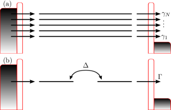
Figure 7: Sketch of the situations that we treat analytically with rate equations. (a) Mutually exclusive channels for the delocalized eigenstates of a monomer chain. The rates $\gamma_{\ell}$ reflect the overlap between the eigenstates and the first and the last site and obey $\sum_{\ell}\gamma_{\ell}=\Gamma$. (b) Two-state model for the edge states in the topological region. The intersite tunneling $\Delta$ is the exponentially small overlap between the edge states given in Eq. (7).

C.2 Two-site model

In the topological region and for a sufficiently long array, the transport occurs mainly via long-range tunneling from one edge state to the other, while the population of the other eigenstates is negligible. Then a proper simplified model is that of a two-level system with tunnel splitting $\Delta$ and a coupling to the source and drain, as is sketched in Fig. 7(b). It can be captured by the master equation (in the basis $\{|0\rangle\langle 0|,|L\rangle\langle L|,|R\rangle\langle R|,|L\rangle\langle R|,|R\rangle\langle L|\}$)

$$\dot{\rho}=\begin{pmatrix}-\Gamma_{L}&0&\Gamma_{R}&0&0\\ \Gamma_{L}&0&0&i\Delta/2&-i\Delta/2\\ 0&0&-\Gamma_{R}&-i\Delta/2&i\Delta/2\\ 0&i\Delta/2&-i\Delta/2&-\Gamma_{R}/2&0\\ 0&-i\Delta/2&i\Delta/2&0&-\Gamma_{R}/2\end{pmatrix}\rho,$$ (20)

In the symmetric case $\Gamma=\Gamma_{R}=\Gamma_{L}$, the current and the Fano factor can be obtained along the lines described in Appendix B as

$$I=\frac{\Gamma\Delta^{2}}{\Gamma^{2}+3\Delta^{2}},$$ (21)

$$F=\frac{\Gamma^{4}+5\Delta^{4}-2\Gamma^{2}\Delta^{2}}{\left(\Gamma^{2}+3\Delta^{2}\right)^{2}}.$$ (22)

In the limit $\Delta\ll\Gamma$, considered in the main text, we expand Eqs. (21) and (22) to second order in $\Delta$ and obtain

$$I=\frac{\Delta^{2}}{\Gamma},$$ (23)

$$\frac{C_{2}}{I}=1-8\frac{\Delta^{2}}{\Gamma^{2}}=F.$$ (24)

Moreover, we perform the iteration scheme for the next cumulants within the same accuracy which provides the expressions

$$\frac{C_{3}}{I}=1-\frac{24\Delta^{2}}{\Gamma^{2}},$$ (25)

$$\frac{C_{4}}{I}=1-\frac{56\Delta^{2}}{\Gamma^{2}}.$$ (26)

Thus, to lowest order in $\Delta$, all cumulants equal the current, which indicates that the transport process is essentially Poissonian.

References

- van der Wiel et al. (2003) W. G. van der Wiel, S. De Franceschi, J. M. Elzerman, T. Fujisawa, S. Tarucha, and L. P. Kouwenhoven, Rev. Mod. Phys. 75, 1 (2003).
- Cuevas and Scheer (2010) J. C. Cuevas and E. Scheer, Molecular Electronics: An Introduction to Theory and Experiment, Series in Nanoscience and Nanotechnology (World Scientific, Singapore, 2010).
- Weinmann et al. (1995) D. Weinmann, W. Häusler, and B. Kramer, Phys. Rev. Lett. 74, 984 (1995).
- Ono et al. (2002) K. Ono, D. G. Austing, Y. Tokura, and S. Tarucha, Science 297, 1313 (2002).
- Busl et al. (2013) M. Busl, G. Granger, L. Gaudreau, R. Sánchez, A. Kam, Pioro-Ladrière, S. A. Studenikin, P. Zawadzki, Z. R. Wasilewski, A. S. Sachrajda, and G. Platero, Nat. Nanotechnol. 8, 261 (2013).
- Weig et al. (2004) E. M. Weig, R. H. Blick, T. Brandes, J. Kirschbaum, W. Wegscheider, M. Bichler, and J. P. Kotthaus, Phys. Rev. Lett. 92, 046804 (2004).
- Koch and von Oppen (2005) J. Koch and F. von Oppen, Phys. Rev. Lett. 94, 206804 (2005).
- Leturcq et al. (2009) R. Leturcq, C. Stampfer, K. Inderbitzin, L. Durrer, C. Hierold, E. Mariani, M. G. Schultz, F. von Oppen, and K. Ensslin, Nature Phys. 5, 327 (2009).
- Barthold et al. (2006) P. Barthold, F. Hohls, N. Maire, K. Pierz, and R. J. Haug, Phys. Rev. Lett. 96, 246804 (2006).
- Sánchez et al. (2008) R. Sánchez, S. Kohler, P. Hänggi, and G. Platero, Phys. Rev. B 77, 035409 (2008).
- Su et al. (1979) W. P. Su, J. R. Schrieffer, and A. J. Heeger, Phys. Rev. Lett. 42, 1698 (1979).
- Zak (1989) J. Zak, Phys. Rev. Lett. 62, 2747 (1989).
- Atala et al. (2013) M. Atala, M. Aidelsburger, J. T. Barreiro, D. Abanin, T. Kitagawa, E. Demler, and I. Bloch, Nature Physics 9, 795 (2013).
- Delplace et al. (2011) P. Delplace, D. Ullmo, and G. Montambaux, Phys. Rev. B 84, 195452 (2011).
- Bello et al. (2016) M. Bello, C. E. Creffield, and G. Platero, Sci. Rep. 6, 22562 (2016).
- Bernevig (2013) B. A. Bernevig, Topological Insulators and Topological Superconductors (Princton University Press, New Jersey, 2013).
- Bagrets and Yu. V. Nazarov (2003) D. A. Bagrets and Yu. V. Nazarov, Phys. Rev. B 67, 085316 (2003).
- Novotný et al. (2004) T. Novotný, A. Donarini, C. Flindt, and A.-P. Jauho, Phys. Rev. Lett. 92, 248302 (2004).
- Flindt et al. (2008) C. Flindt, T. Novotný, A. Braggio, M. Sassetti, and A.-P. Jauho, Phys. Rev. Lett. 100, 150601 (2008).
- Ya. M. Blanter and Büttiker (2000) Ya. M. Blanter and M. Büttiker, Phys. Rep. 336, 1 (2000).
- Kaiser et al. (2006) F. J. Kaiser, M. Strass, S. Kohler, and P. Hänggi, Chem. Phys. 322, 193 (2006).
- Kießlich et al. (2007) G. Kießlich, E. Schöll, T. Brandes, F. Hohls, and R. J. Haug, Phys. Rev. Lett. 99, 206602 (2007).
- Anderson (1958) P. W. Anderson, Phys. Rev. 109, 1492 (1958).
- Puddy et al. (2015) R. K. Puddy, L. W. Smith, H. Al-Taie, C. H. Chong, I. Farrer, J. P. Griffiths, D. A. Ritchie, M. J. Kelly, M. Pepper, and C. G. Smith, Appl. Phys. Lett. 107, 143501 (2015).
- Kocić et al. (2015) N. Kocić, P. Weiderer, S. Keller, S. Decurtins, S.-X. Liu, and J. Repp, Nano Lett. 15, 4406 (2015).
- Gómez-León and Platero (2013) A. Gómez-León and G. Platero, Phys. Rev. Lett. 110, 200403 (2013).
- Domínguez et al. (2010) F. Domínguez, G. Platero, and S. Kohler, Chem. Phys. 375, 284 (2010).