Hořava’s quantum gravity illustrated
by embedding diagrams of the Kehagias-Sfetsos spacetimes

Abstract

Possible astrophysical consequences of the Hořava quantum gravity theory have been recently studied by several authors. They usually employ the Kehagias-Sfetsos (KS) spacetime which is a spherically symmetric vacuum solution of a specific version of Hořava’s gravity. The KS metric has several unusual geometrical properties that in the present article we examine by means of the often used technique of embedding diagrams. We pay particular attention to the transition between naked singularity and black-hole states, which is possible along some particular sequences of the KS metrics.

1 Introduction

Black holes almost certainly exist in the real universe. In studying their properties, astrophysicists usually use two famous exact solutions of Einstein’s field equations of his general relativity theory — the Schwarzschild solution that describes a static, spherically symmetric gravity of a non-rotating black hole, and the Kerr solution which describes a stationary, axially symmetric gravity of a rotating black hole. The Reissner-Nordström solution which describes a static, spherically symmetric gravity of a charged, non-rotating black hole is considered to be astrophysically unrealistic, because charged macroscopic objects quickly neutralize by accreting plasma of the opposite sign. The Schwarzschild and Kerr black holes are now quite familiar objects in astrophysics.

However, black holes in the real universe may be different from those of the Schwarzschild or of the Kerr type. First, Einstein’s theory of gravitation has not yet been tested in its strong field limit relevant to black holes. A variety of alternative gravity theories were studied and theoretically and observationally tested, in the strong gravity limit. Firstly, there is a number of papers related to braneworld black holes dad-etal:2000:PLB: ; ali+gun:2005:PRD: ; Sche-Stu:2013:JCAP: or stringy black holes gib+mae:1988:NPB: ; sen:1992:PRL: ; has+sen:1992:NP: ; bla+bla:2001:CQG: ; hio+miy:2008:PRD: . On the other hand, there is an extensive study of regular black holes where general relativity is combined with non-linear electrodynamics bar:1968: ; ayo+gar:1998:PRL: ; ayo:1999:PLB: ; ayo+gar:1999:GRG: ; ayo+gar:2000:PLB: ; sche+stu:2015:IJMP: ; sche+stu:2015:JCAP: ; gho+man:2015:EPJ: . Inspired by some ideas of quantum theory, static and rotating, regular (i.e. singularity-free), black hole spacetimes have been proposed dym:1992:GRG: ; mod:2004:PRD: ; nic-etal:2006:PLB: ; bam:2013:PRD: ; li+bam:2013:PRD: ; liu-etal:2014:PRD: ; bam-etal:2014:EPJC: ; dym+gal:2015:CQG: , and also their behavior due to gravitational collapse has been studied zha-etal:2015 . The solution representing regular black holes in the de Sitter universe has been found in mat-etal:2008:MPLA: . Alternatively, string theory could allow for existence of superspinars gim+hor:2009:PLB: ; stu+schee:2013:CQG: . Secondly, although the quantum gravity theory is still unknown, there are numerous hints that quantum effects may influence strong gravity. Several attempts have been made to describe this influence. Hořava’s theory Hor:2009:PHYSR4: ; Hor:2009:PHYSRL: is a particular recent example. Like some other quantum gravity theories, it points to interesting possibilities that may be directly relevant to astrophysics: (a) the existence of naked singularities with observational consequences that may be calculated, (b) a dynamical phenomenon of “antigravity” Vieira:2014:PHYSR4: . It seems that these two features are genuine for a wide class of Einsteinian (e.g., Reissner-Nordström) and non-Einsteinian (e.g., quantum) strong gravitational fields. In this paper we discuss these phenomena specifically for the Hořava gravity, in terms of embedding diagrams. The embedding diagrams help to build intuition about strongly curved spacetime geometry, which is equivalent to strong gravity.

2 Hořava’s quantum gravity

Hořava Hor:2009:PHYSR4: ; Hor:2009:PHYSRL: proposed a new approach to quantum gravity that is a field theory based on solid state physics ideas lif:1941 , being invariant under Lifshitz scaling ($t\rightarrow\beta^{z}t,x\rightarrow\beta x$), with the dynamical critical exponent $z$ flowing from $z=3$ in the short wavelength UV limit, to the value $z=1$ in the large wavelength IR limit. The theory “could therefore serve as a UV completion of Einstein’s general relativity” Hor:2009:PHYSR4: . Gravity is an emergent property of the IR limit of the theory; thus Newton’s constant is given by a constant of the theory $\kappa$, through $G=\kappa^{2}/32\pi c$, $c$ is being the speed of light. In this field-theoretical version of quantum gravity the field equations are derived from a Lagrangian that guarantees Lorentz invariance (and no preferred time) at low energies, but no Lorentz invariance (and a preferred time) at high energies. Because of different scaling between time and space, the Hořava quantum gravity action at UV limit is not invariant under general relativistic diffeomorphisms, but it has to be invariant under a diffeomorphism preserving foliations: $t\rightarrow t_{\ast}(t)$, $x^{i}\rightarrow x^{i}_{\ast}(t,x^{i})$. The space and time are treated differently in Hořava gravity, then Lorentz violation occurs at all scales at the UV regime, but vanishes in the IR general relativistic limit.

Soon after, Kehagias and Sfetsos Keh-Sfe:2009:PhysLetB: derived and solved a modified version of Hořava’s field equations for the spherically symmetric, static (i.e. a “Schwarzschild-like”) case. We will call it the KS spacetime (or the KS metric) for short. Writing

$$ds^{2}=-N^{2}dt^{2}+g_{ij}(dx^{i}+N^{i}dt)(dx^{j}+N^{j}dt)$$ (1)

and discarding the cosmological term, the authors of Ref. Keh-Sfe:2009:PhysLetB: considered the action of modified Hořava gravity

$$S= \int dtd^{3}x\sqrt{g}N\{\frac{2}{K^{2}}\left(K_{ij}K^{ij}-\lambda K^{2}\right)-\frac{\kappa^{2}}{2\nu^{4}}C_{ij}C^{ij}$$ (2)

$$+\frac{\kappa^{2}\mu}{2\nu^{2}}\epsilon^{ijk}R_{il}^{(3)}\nabla_{j}R^{(3)l}_{\,\,\,\,\,\,\,\,\,k}-\frac{\kappa^{2}\mu^{2}}{8}R_{ij}^{(3)}R^{(3)ij}$$

$$+\frac{\kappa^{2}\mu^{2}}{8(1-3\lambda)}\frac{1-4\lambda}{4}\left(R^{(3)}\right)^{2}+\mu^{4}R^{(3)}\},$$

where $K_{ij}=(\dot{g}_{ij}-\nabla_{i}N_{j}-\nabla_{j}N_{i})/(2N)$ is the extrinsic curvature of the $t=const$ hypersurfaces and $C^{ij}=\epsilon^{ikm}\nabla_{k}(R^{(3)j}_{\,\,\,\,\,\,\,\,\,m}-R^{(3)}\delta_{m}^{j}/4)$ is the Cotton tensor, $R^{(3)}$ is the 3-D Ricci scalar of the hypersurfaces. The constants $\kappa,\nu$ and $\lambda$ are dimensionless, while the constant $\mu$ has mass dimension 1. The terms involving $\nu$ vanish in the spherically symmetric case Keh-Sfe:2009:PhysLetB: .

In this paper we discuss some extreme geometrical properties of the KS spacetimes that may be relevant for astrophysics. While Hořava’s theory itself is not generally covariant, our calculations in the KS metric are — they fulfill the standard rules of a covariant theory familiar from Einstein general relativity. The KS spherically symmetric solution is asymptotically flat in the $\lambda=1$ case, with $N_{i}=0$, and $N^{2}=1/{|g_{rr}|}\equiv f$, where $f$ is the so called lapse function of the spacetime. The obtained solution contains the parameter $\omega=16\mu^{2}/\kappa^{2}>0$, in addition to the gravitational mass $M$, and tends to the Schwarzschild solution in the limit of the dimensionless parameters product $\omega M^{2}\rightarrow\infty$ (expressed in geometrized units). Presumably, $\omega$ is a universal constant, if the KS solution correctly describes the gravity of spherically symmetric objects. For large masses, $\omega M^{2}>1/2$, the Kehagias-Sfetsos solution has event horizons and corresponds to a black hole Keh-Sfe:2009:PhysLetB: . The current observational (lower) limits on $\omega$ are compatible with the existence of naked singularities at masses $M<2.6\times 10^{4}\,M_{\odot}$ Ior+rug:2010:IJMP: ; liu-etal:2011:GRG: ; har-etal:2011:PRCA: .

We conduct our discussion in terms of the embedding diagrams of the KS metric “equatorial planes”. The KS geometry is spherically symmetric, and therefore the geometry of all central planes is the same as that of the equatorial plane. This allows us to consider, with no loss of generality, these particular embedding diagrams as a faithful representation for the whole KS geometry. A similar approach was used previously, for different spacetimes, by several authors. For example, Kristiansson et al. Kri-Son-Abr:1998:GRG: analyzed embedding of the Reissner-Nordström (RN) 3-spaces. This work is particularly relevant in the present context. We will see later that RN and KS metrics share several interesting properties that nicely show up in the embeddings.

We use here the standard embeddings of the conventional “physical”, i.e. a simply projected 3-D space but also less standard embeddings of a projected and in addition conformally re-scaled “optical” 3-D space. The optical geometry reflects directly some dynamical properties of the particle and photon motion. For example, geodesic lines in the KS optical 3-D space coincide with the photon trajectories.

3 The Kehagias-Sfetsos spacetime

An important class of static and spherically symmetric spacetimes has a general form,

$$\mathrm{d}s^{2}=-f(r)\mathrm{d}t^{2}+\frac{1}{f(r)}\mathrm{d}r^{2}+r^{2}\mathrm{d}\theta^{2}+r^{2}\sin^{2}\theta\mathrm{d}\phi^{2}.$$ (3)

The “simply projected” 3-D space at a given time $t$, is defined by a $t$$=$ const section of the spacetime. In this 3-D space, one may define the “equatorial plane” by $\theta$$=$$\pi/2$. It has the intrinsic metric

$$\mathrm{d}\ell^{2}=\frac{1}{f(r)}\mathrm{d}r^{2}+r^{2}\mathrm{d}\phi^{2}.$$ (4)

In the classic (non-quantum) Einstein gravity, for all the static, vacuum, spherically symmetric and asymptotically flat spacetimes, the lapse function $f(r)$ must be necessarily given by its “Schwarzschild” form,

$$f(r)=1-\frac{2M}{r},$$ (5)

where $M$ is the mass in “geometrical” units of length, $c\,$$=\,$$1\,$$=\,$$G$.

Kehagias and Sfetsos Keh-Sfe:2009:PhysLetB: found that in the quantum-gravity version of (3)-(5) one should only modify the lapse function $f(r)$,

$$f(r)=1+r^{2}\omega\left(1-\sqrt{1+\frac{4M}{\omega r^{3}}}\right).$$ (6)

Here $\omega$ is a physical constant (a quantum-gravity parameter) of dimension [cm^-2]. It is easy to see that one recovers the classic Schwarzschild solution (5) when one puts, in the KS solution (6) for the $f(r)$ function, $\omega\rightarrow\infty$.

The location of the event horizon is given for a static metric by $g_{tt}\equiv f(r)=0$, which for the KS solution yields Keh-Sfe:2009:PhysLetB:

$$\left(\frac{r}{M}-1\right)^{2}=1-\frac{1}{2\omega M^{2}}.$$ (7)

Clearly, there are two horizons, inner and outer, of the KS black hole spacetimes if

$$\omega>\omega_{c}=\frac{1}{2M^{2}}.$$ (8)

For $\omega<\omega_{c}$ a naked KS singularity occurs at $r=0$, where the Ricci and Riemann tensor components behave as (see Keh-Sfe:2009:PhysLetB: ),

$$[{\rm Ricci,~{}Riemann}]\sim\frac{1}{r^{3/2}}\sim\infty.$$ (9)

Note that the KS metric is not Ricci flat. Instead, one has (for large $\omega$),

$$[{\rm Ricci}]\sim\frac{1}{\omega}+{\cal O}(\frac{1}{\omega^{2}})\,.$$ (10)

For more details see (stu-sche-apt:2014 ). It is convenient to write the metric (3) in the form,

$$\mathrm{d}s^{2} = \mathrm{e}^{-2\Phi(r)}\,\mathrm{d}s^{2}_{*},\qquad\Phi(r)=-\frac{1}{2}\,\ln f(r),$$ (11)

$$\mathrm{d}s^{2}_{*} = -\mathrm{d}t^{2}+\frac{1}{[f(r)]^{2}}\mathrm{d}r^{2}+\frac{r^{2}}{f(r)}\mathrm{d}\theta^{2}+\frac{r^{2}\sin^{2}\theta}{f(r)}\mathrm{d}\phi^{2}.$$ (12)

The ultra-static metric (12), which is conformal to the original metric (3) is often called the “optical geometry” metric. The reason for this name follows from the fact that light trajectories are not only (null) geodesics in the four-dimensional spacetime, but they are also space-like geodesics in the 3-D space of the optical geometry (12). This property is useful in studying the motion of particles and photons, as often non-trivial information may be easily deduced directly from the geometry, in particular the geometry of embedding diagrams. This is why the optical geometry embeddings are helpful in building physical intuition and therefore worth studying. From (12) one deduces that the line element on the 2-D equatorial plane in the KS optical space is given by

$$\mathrm{d}\ell^{2}=\frac{1}{[f(r)]^{2}}\mathrm{d}r^{2}+\frac{r^{2}}{f(r)}\mathrm{d}\phi^{2}.$$ (13)

4 The embedding procedure

Note that the line element on the 2-D equatorial plane in both the simply projected space (4) and the optical space (13), may be put in the form

$$\mathrm{d}\ell^{2} = g_{rr}(r)\,\mathrm{d}r^{2}+g_{\phi\phi}(r)\,\mathrm{d}\phi^{2}$$ (14)

$$= \mathrm{d}r_{*}^{2}+{\tilde{r}}^{2}\,\mathrm{d}\phi^{2},$$

where $r_{*}$ is the “geodesic” and $\tilde{r}$ the “circumferential” radius of an $r$ $=$ const circle. These two radii are defined by

$$r_{*}(r)=\int\sqrt{g_{rr}}\,\mathrm{d}r,\qquad{\tilde{r}}(r)=\sqrt{g_{\phi\phi}}.$$ (15)

Thus, in the simply projected metric we have

$$r_{*}(r)=\int{\frac{1}{[f(r)]^{1/2}}}\,\mathrm{d}r,\qquad{\tilde{r}}(r)=r,$$ (16)

and in the optical geometry we have

$$r_{*}(r)=\int{\frac{1}{f(r)}}\,\mathrm{d}r,\qquad{\tilde{r}}(r)=\frac{r}{\sqrt{f(r)}}.$$ (17)

The curvature ${\cal K}$ of an $r$ $=$ const circle and the Gaussian curvature of the equatorial plane at the circle are given by

$${\cal K}=+\frac{1}{\tilde{r}}\left(\frac{\mathrm{d}{\tilde{r}}}{\,\mathrm{d}r_{*}}\right),\qquad{\cal G}=-\frac{1}{\tilde{r}}\left(\frac{\mathrm{d}^{2}{\tilde{r}}}{\mathrm{d}r_{*}^{2}}\right).$$ (18)

The curvature radius of the circle is defined as ${\cal R}=1/{\cal K}$. The Gaussian curvature ${\cal G}$ has the dimension of [cm^-2].

In the embedding procedure, one determines a function

$$Z=Z(R),$$ (19)

such that in the 3-D Euclidean space

$$\mathrm{d}\ell^{2}=\mathrm{d}R^{2}+\mathrm{d}Z^{2}+R^{2}\,\mathrm{d}\phi^{2}$$ (20)

the 2-D surfaces $Z=Z(R)$ have the same intrinsic geometry,

$$\mathrm{d}\ell^{2}=\left[1+\left(\frac{\mathrm{d}Z}{\mathrm{d}R}\right)^{2}\right]\mathrm{d}R^{2}+R^{2}\,\mathrm{d}\phi^{2},$$ (21)

as the intrinsic geometry on the equatorial plane

$$\mathrm{d}\ell^{2}=\mathrm{d}r_{*}^{2}+{\tilde{r}}^{2}\,\mathrm{d}\phi^{2}.$$ (22)

Equating expressions (21) and (22) one gets equations which determine the embedding function in the parametric form $Z=Z(R(r))$, with $r$ being the parameter,

$$\left[1+\left(\frac{\mathrm{d}Z}{\mathrm{d}R}\right)^{2}\right]^{1/2}\mathrm{d}R=\mathrm{d}r_{*}(r),\qquad R={\tilde{r}}(r).$$ (23)

The explicit solution for $\mathrm{d}Z(r)/\mathrm{d}r$ follows after short algebra,

$$\frac{\mathrm{d}Z}{\mathrm{d}r} = \frac{\mathrm{d}R}{\mathrm{d}r}\sqrt{\left(\frac{\mathrm{d}r_{*}}{\mathrm{d}r}\right)^{2}\left(\frac{\mathrm{d}{\tilde{r}}}{\mathrm{d}r}\right)^{-2}-1},$$ (24)

$$\frac{\mathrm{d}R}{\mathrm{d}r} = \frac{\mathrm{d}{\tilde{r}}}{\mathrm{d}r}.$$ (25)

The functions $r_{*}(r)$ and ${\tilde{r}}(r)$ are given in terms of $g_{rr}$ and $g_{\phi\phi}$ by Eq. (15), and $g_{rr}(r)$ and $g_{\phi\phi}(r)$ are given by Eqs. (4), (13) in terms of the function $f(r)$, which is itself given by (6). Knowledge of these functions allows one to directly integrate (24) numerically and obtain the embedding profile $Z(R)$.

Eqs. (24)-(25) do not always determine directly a function $Z(R)$, because the relation $F(R,Z)$ is multi-valued and does not determine a unique mapping $R\rightarrow Z$. This is never a problem in practice, however, as it is always obvious which specific map should be chosen. The specific choice defines uniquely the relation, indeed a function, $Z(R)$. It is this function which we have in mind here. This remark concerns mostly the region between the “turning points” in the optical space embedding (which we discuss later).

Note that (24) may be also written as

$$\frac{\mathrm{d}Z}{\mathrm{d}R}=\frac{1}{{\tilde{r}}}\sqrt{{\cal R}^{2}-{\tilde{r}}^{2}}=\frac{1}{{\tilde{r}}}\sqrt{[{\cal R}-{\tilde{r}}][{\cal R}+{\tilde{r}}]}\,.$$ (26)

Because ${\cal R}$ and ${\tilde{r}}$ are (by definition) non-negative, the condition that the function under the square root in Eq. (26) be non-negative reads

$${\cal R}\geq{\tilde{r}}.$$ (27)

If condition (27) is not fulfilled, then the embedding in the 3-D Euclidean space is not possible. One knows that ${\rm sign}({\cal G})=-{\rm sign}(\mathrm{d}^{2}{\tilde{r}}/\mathrm{d}r^{2})$. It follows that the Gaussian curvature of the embedded surfaces changes sign as $Z$ increases, both in simply projected and optical spaces, being always positive in the anti-gravity region. This change of sign does not depend on the existence of photon orbits, since it appears for all values of $\omega$ (see for instance Fig. 2 for the simply projected case and Figs. 5, 6, 7 for the optical case).

5 Embedding of the KS equatorial plane

For simplicity of notation, we will use from now on a re-scaled (dimensionless) version of the quantum parameter $\omega$. The re-scaling is defined by $\omega M^{2}\rightarrow\omega$. Similarly, we re-scale length, $x=\{r,R,{\tilde{r}},Z,...\}$, by $x\rightarrow x/M$. There is no danger of confusion between the two versions of $\omega$ and $x$, so we will use the same symbols for both of them. For example, the critical value of $\omega$ defined by (8) may be simply written as $\omega_{c}=1/2$.

5.1 The case of a simply projected space, Eq. (4)

By using the procedure described in the previous Section, we derive for the function $Z=Z(r)$ that determines the shape of the embedding profile,

$$\frac{\mathrm{d}Z}{\mathrm{d}r}=\sqrt{\frac{-r^{2}\omega\left(1-\sqrt{1+\frac{4}{\omega r^{3}}}\,\right)}{1+r^{2}\omega\left(1-\sqrt{1+\frac{4}{\omega r^{3}}}\,\right)}},\qquad r=R.$$ (28)

In the case of the black hole, i.e. $\omega>1/2$, the whole region $r_{+}<r<\infty$ can be embedded (from the outer horizon to infinity), as the condition (27) is fulfilled everywhere. The region $0<r<r_{-}$ can also be embedded. We show examples of this embedding in Fig. 1.

For naked singularities, $\omega<\omega_{c}$, one can construct embedding diagrams for the entire range of the radial coordinate $0<r<\infty$. Examples are presented in Fig. 2.

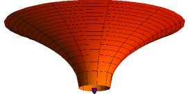
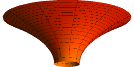
Figure 1: Embedding diagrams for the equatorial plane in the simply projected 3-D space of the KS black hole spacetime. The left column shows the function $Z(R)$, the right column shows the 2-D curved equatorial plane embedded into the 3-D Euclidean space. Top diagrams are constructed for $\omega=1$ and the bottom ones for $\omega=5$. The “outer” part of the equatorial plane ends at the location of the outer horizon. There is also the “inner” part of the equatorial plane, corresponding to the 3-D space inside the inner horizon. The embedded antigravity region is painted dark violet. As the circumferential radii of the outer and inner horizons are different, there is a clearly visible discontinuity in geometry.

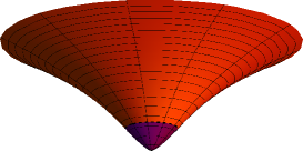
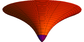
Figure 2: Embedding diagrams for the equatorial plane in the simply projected 3-D space of the KS naked singularity spacetime. The top diagram corresponds to $\omega=0.1$ and the bottom one to $\omega=0.3$. The embedded surfaces go all the way to $r=0$, i.e. the location of the naked singularity (the lowest central point on the surfaces).

5.2 The case of the optical space, Eq. (13)

In this case, the embedding profile is given by equations,

$$\frac{\mathrm{d}Z}{\mathrm{d}r} = f^{-1}(r)\sqrt{1-f^{-1}(r)\left[1-\frac{3}{r}\left(1+\frac{4}{\omega r^{3}}\right)^{-\frac{1}{2}}\right]^{2}},$$ (29)

$$\frac{\mathrm{d}R}{\mathrm{d}r} = f^{-3/2}(r)\left[1-\frac{3}{r}\left(1+\frac{4}{\omega r^{3}}\right)^{-1/2}\right],$$ (30)

$$R = \frac{r}{\sqrt{f(r)}}\,.$$ (31)

The “turning points” of the embedding profile are given by the condition

$$\frac{\mathrm{d}R}{\mathrm{d}r}=0.$$ (32)

According to (18) they are spacelike geodesic circles, and therefore they correspond to the location of circular photon orbits in the KS spacetime.

From Eq. (29), we can see that embedding is possible if

$$1-f^{-1}(r)\left[1-\frac{3}{r}\left(1+\frac{4}{\omega r^{3}}\right)^{-\frac{1}{2}}\right]^{2}\geq 0.$$ (33)

5.3 Three classes of embedding diagrams

In terms of $\omega$, the locations of horizons [given by Eq. (7)], turning points [given by Eq. (32)], and the limits on the embedding procedure [given by Eq. (33)] are shown in Fig. 3. The Figure suggests that there are three classes of embedding diagrams in optical geometry:

class 1: The range $\omega<\frac{1}{3}\sqrt{\frac{4}{3}}$ corresponds to naked singularities. No horizons are present. There are no turning points or embedability limits, either. The whole region from $r=0$ to infinity can be embedded. Examples of embedding diagrams of this class are pictured in Fig. 5.

class 2: The range $\frac{1}{3}\sqrt{\frac{4}{3}}\leq\omega<\frac{1}{2}$ corresponds to naked singularities as well. However, turning points exist. Embedding diagrams for this class are shown in Fig. 6.

class 3: The range $\omega>1/2$. The object is a black hole and there are horizons. Also, limits on embedability and turning points are present. There is always an embedability limit outside the outer horizon. Embedding diagrams for this class are shown in Fig. 7.

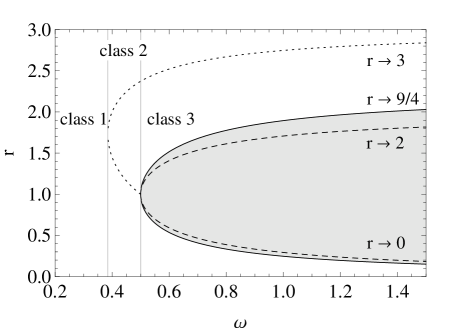
Figure 3: Relevant radii in KS spacetime. The long-dashed line shows location of the horizons. It is given by Eq. (7). The short-dashed line shows the location of turning points in the optical geometry. It is given by Eq. (32). The solid line shows limits on embedability (in the optical geometry case). It is given by Eq. (33). The shaded region cannot be embedded. Numbers near the right axis show the asymptotic ($\omega\rightarrow\infty$) behavior of the corresponding curves. The vertexes of the (horizontal) “parabolas” that these three lines represent are at $(\omega,r)=(\frac{1}{3}\sqrt{\frac{4}{3}},\sqrt{3})$ and $(\omega,r)=(\frac{1}{2},1)$. These two locations define the split of the parameter space into three classes, as shown by vertical lines and labels, and as described in the text.

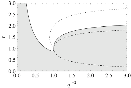
Figure 4: Relevant radii in Reissner-Nordström spacetime. The lines and the shaded area have the same meaning as in Fig. 3. The radial coordinate is re-scaled as $r\to r/M$ and the charge parameter is $q=Q/M$. We see that the radii corresponding to turning points and horizons have the same qualitative behavior as in KS spacetime, however the embedability conditions are qualitatively different.

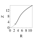
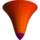
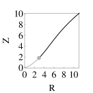
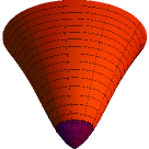
Figure 5: Class 1 of the embedding diagrams (a naked singularity). The optical geometry case is shown. Top: $\omega=0.2$. Bottom: $\omega=0.05$. The left column shows the circumferential radius $R(r)$, the middle column the embedding profile $Z(R)$, and the right column the embedded surface. The grey color at the profile shows the antigravity region, the grey point shows the location of the zero-gravity sphere. The antigravity region is indicated by a dark violet color in the embedded surface. See subsection 6.2 for a more detailed explanation.

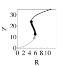
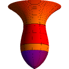
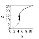
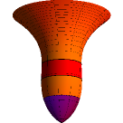
Figure 6: Class 2 of the embedding diagrams (naked singularity). The optical geometry case is shown. Top: $\omega=0.45$. Bottom: $\omega=0.4$. The left column shows the circumferential radius $R(r)$, the middle column the embedding profile $Z(R)$, and the right column the embedded surface. The grey color at the profile shows the antigravity region, the large grey dot shows the location of the zero-gravity sphere. The region where centrifugal force is reversed is shown in red. The antigravity region is indicated by a dark violet color in the embedded surface. The dark large dots show the locations of the turning points. They correspond to the circular photon orbits. The photon orbits are indicated by solid circles at the embedded surface. See subsection 6.2 for a more detailed explanation.

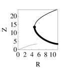
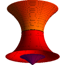
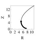
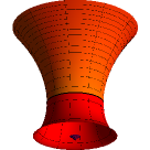
Figure 7: Class 3 of the embedding diagrams (black hole). The optical geometry case is shown. Top: $\omega=0.55$. Bottom: $\omega=1.00$. The colors and curves have the same meaning as in Fig. 6. There are two disconnected “spaces” here: the “outer” space outside the outer horizon, and the “inner” space inside the inner horizon and around the central singularity. Note that the embedding diagrams do not end at the inner and outer horizons, but at radii corresponding to the embedability limits, which are located close to the horizons. Near embedability limits, the embedding diagrams have horizontal asymptotes, as $\mathrm{d}Z/\mathrm{d}R=0$. This cannot be nicely illustrated. Thus, in the Figure, the surfaces stop slightly before the embedability limits.

6 Discussion

6.1 Comparison between KS and Reissner-Nordström cases

As mentioned before, the qualitative properties of the KS solution resemble those of Reissner-Nordström spacetime. In particular, we see from Fig. 4 that the radii corresponding to horizons and photon orbits have the same structure in both spacetimes, when instead of $\omega$ the horizontal axis displays $q^{-2}$, where $q=Q/M$ is the charge-to-mass parameter in RN spacetime. The antigravity radius also has a similar behavior in both cases, meaning that in the naked-singularity region it is always positive and goes to infinity if the parameter of Fig. 3 or Fig. 4 goes to zero, whereas in the black-hole region the static region between the singularity and the inner horizon is of antigravity. The difference appears in the embedding limits for optical (and simply projected) geometry, as first discussed in Kri-Son-Abr:1998:GRG: . As shown in Fig. 4 for optical geometry, in the black-hole case the inner region can be embedded only in KS spacetime. Also, the embedability limit in RN is always below the antigravity radius for the naked-singularity case.

Concerning the simply projected geometry, while in KS spacetime embedability is always possible in static regions, Eqs. (16) and (24) imply that the embedability condition in RN is given by $r\geq q^{2}/2$, and since the horizons are given by $r_{\pm}=1\pm\sqrt{1-q^{2}}$ there is, in the black-hole case, a region inner to $r_{-}$ (the inner horizon) which can be embedded. However, this region never extends up to the singularity. In the naked-singularity case the embedability limit is always below the antigravity radius, which is given by $r=q^{2}$.

6.2 Antigravity and centrifugal force reversal

In the original “physical” spacetime (3), one considers a general circular motion, with the four-velocity,

$$\frac{\mathrm{d}x^{i}}{\mathrm{d}s}=u^{i}=\gamma\left(N^{i}+v\tau^{i}\right),$$ (34)

where $N^{i}$ is a timelike unit vector in the $t$ direction, and $\tau^{i}$ is a spacelike unit vector in the $\phi$ direction. We will define the orbital velocity $V=\gamma v$. The acceleration in circular motion equals

$$a_{i}=u^{k}\nabla_{k}u_{i}=g_{i}+c_{i},$$ (35)

where the “gravitational” and “centrifugal” accelerations are given by formulae which refer (formally) to the optical space,

$${\rm gravitational} \qquad g_{i}=N^{k}\nabla_{k}N_{i}=\nabla_{i}\Phi,\qquad\Phi=-\frac{1}{2}\ln f,$$ (36)

$${\rm centrifugal} \qquad c_{i}=\frac{\,\,V^{2}}{\cal R}\,\lambda_{i},\qquad\lambda_{i}=\frac{\nabla_{i}{\tilde{r}}}{[(\nabla_{k}{\tilde{r}})(\nabla^{k}{\tilde{r}})]^{1/2}}\,.$$ (37)

We stress that $g_{i}$ and $c_{i}$ “live” in the original “physical” spacetime, and that the reference to the optical space is made here mostly for a formal convenience.

Not only for convenience, however. This reference also helps to strengthen a physical intuition, as we will see later when discussing the embedding diagrams of the KS optical space.

In the above formulae (36)-(37), the “gravitational potential” $\Phi$ is given by the optical space conformal factor (11), and both the curvature radius of the orbit ${\cal R}$ and the unit space-like vector orthogonal to the trajectory $\lambda_{i}$ are defined (and calculated) in the optical space.

For the free, geodesic circular orbits it should be $a_{i}=0$. Therefore a necessary condition for the existence of the geodesic orbit is that the gravitational and centrifugal accelerations point to the opposite radial directions,

$$g_{i}c^{i}<0$$ (38)

in the optical space. In a situation familiar from Newtonian physics, gravity always pulls inwards and the centrifugal force always pushes out, and therefore the condition (38). In KS spacetimes the situation is more complex, as two rather unusual effects are present: antigravity and centrifugal force reversal.

Let us define the “signs” of gravitational and centrifugal accelerations by

$$[g]={\rm sign}(g^{i}k_{i}),~{}~{}[c]={\rm sign}(c^{i}k_{i}),\qquad{\rm where}~{}~{}k_{i}=\nabla_{i}r.$$ (39)

It should be obvious that gravity pulls in, pushes out or vanishes depending on the sign of $[g]$,

$$\hskip-0.28436pt[g]=\left\{\begin{array}[]{ll}+1&\mbox{gravity pushes out (``antigravity'')}\\ ~{}~{}0&\mbox{gravity vanishes}\\ -1&\mbox{gravity pulls in }\end{array}\right.$$ (40)

and that the same is true for the centrifugal force,

$$\hskip-0.28436pt[c]=\left\{\begin{array}[]{ll}+1&\mbox{centrifugal force pushes out}\\ ~{}~{}0&\mbox{centrifugal force vanishes}\\ -1&\mbox{centrifugal force pulls in (``reversal'')}\end{array}\right.$$ (41)

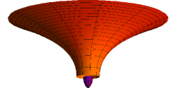
$\omega=0.600$
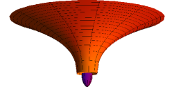
$\omega=0.550$
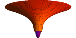
$\omega=0.525$
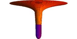
$\omega=0.500$
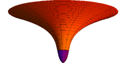
$\omega=0.475$
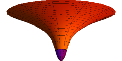
$\omega=0.450$
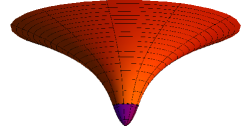
$\omega=0.400$

Figure 8: A sequence of KS objects in simply projected space, showing a transition between the naked singularity and the black hole state (from bottom to top along the sequence shown in the Figure). The transition is a discontinuous one. For $\omega<1/2$ there is no horizon, and at $\omega=1/2$ a finite-size horizon is formed. Its location is shown by a black dot and a solid line in the $\omega=0.500$ panel.

In the embedding diagrams, the region of antigravity, close to the naked singularity at $r=0$ is represented by a strong violet color, and the sphere (a circle on the equatorial plane) of zero gravity is shown in the embedding profiles by light grey. In the region of antigravity the centrifugal force also pushes out, so condition (38) is not fulfilled—free circular (geodesic) orbits are not possible there. Also note that, in the black-hole case, the whole region between the singularity and the inner horizon is an antigravity region—free circular (geodesic) orbits are not possible there.

The centrifugal force reversal happens in the region where, in optical geometry, the circumferential radius ${\tilde{r}}=R$ decreases in the direction of increasing $r_{*}$, colored red in Figs. 6, 7. In these regions the gravitational force pulls in, so condition (38) is not fulfilled — free circular orbits are not possible there. The centrifugal force vanishes (for any finite value of the orbital velocity $V$) at the turning points where ${\tilde{r}}=R$ has a local extremum (minimum or maximum). The minima corresponds to unstable, and maxima to stable circular photon orbits. These orbits are distinguished by solid circles in the optical geometry embedding diagrams.

7 Conclusions

We have discussed geometrical properties of KS spacetimes in terms of embedding diagrams. The KS metric describes a static, spherically symmetric spacetime in the Hořava quantum gravity theory. The non-Einsteinian (quantum) features of the metric are governed by a single parameter $\omega$, which has dimension [cm]^-2. The central KS object, with mass $M$ corresponds to either a black hole (when $\omega M^{2}>1/2$) or a naked singularity (when $\omega M^{2}<1/2$).

We show that a (hypothetical) transition from a naked singularity to a black hole state may be discontinuous, as clearly demonstrated by a sequence of KS spacetimes (Fig. 8), with the horizon size starting from a finite value. This may have an observable astrophysical signature. A similar discontinuity may occur also in the case of the conversion of a Kerr naked singularity into a near-extreme Kerr black hole Stu:1980:Bull.Astr.Inst.Czechoslov: .

We also discussed the phenomena of antigravity and of centrifugal force reversal present in the KS spacetimes. The first one is present for naked singularities, but not outside black holes, the latter for both naked singularities and black holes.

Appendix A Reference guide to Hořava’s gravity

Here we give some additional references that may be useful in the context of our article.

The Hořava gravity (or “Hořava-Lifshitz” gravity as it is often called) is considered as one of the most promising approaches to the quantum gravity. (see And-etal:2012:PHYSR4: ; Gri-Hor-MelT:2012:JHEP: ; Gri-Hor-MelT:2013:PHYSRL: ; Hor:2009:PHYSR4: ; Hor:2009:PHYSRL: ; Hor-MelT:2010:PHYSR4: ; Lib-Mac-Sot:2012:PHYSRL: ; Ver-Sot:2012:PHYSR4: ).

The solutions of the Hořava-Lifshitz effective gravitational equations have been found in Bar-Sot:2012:PHYSRL: ; Bar-Sot:2013:PHYSRL: ; Bar-Sot:2013:PHYSR4: .

The spherically symmetric solution of the Schwarzschild character has been found in the framework of the modified Hořava model and are given by the Kehagias-Sfetsos (KS) metric, which allows for existence of both black hole and naked singularity spacetimes. (see Keh-Sfe:2009:PhysLetB: ; Mu-In:2009:JHEP: ).

In connection to the accretion phenomena, the KS metric has been extensively studied in a series of works related both to the particle motion and optical phenomena (the last two references below) that can be relevant for tests of validity of the Hořava-Lifshitz gravity. Here we demonstrate the properties of the KS spacetime using the embedding diagrams of both the direct geometry and the optical geometry reflecting some hidden properties of the spacetime and its geodetic structure. (see Abd-Ahm-Hak:2011:PHYSR4: ; Ali-Sen:2010:PHYSR4: ; Ata-Abd-Ahm:2013:AstrSpaScie: ; Eno-etal:2011:PHYSR4: ; Hak-etal:2010:MPLA: ; Hak-Abd-Ahm:2013:PHYSR4: ; Hor-Ger-Ker:2011:PHYSR4: ).

In this paper we discussed not only the KS black holes, but also the KS naked singularities. Some phenomena found in the KS naked singularities are similar to these found for the Reissner-Nordström naked singularities, (e.g Stu-Hed:2002:APS: ), the braneworld naked singularities (e.g Ali-etal:2013:CLAQG: ; Stu-Kol:2012:JCAP: ; Stu-Kot:2009:GenRelGrav: )and the Kerr naked singularities (e.g Pat-Jos:2011:CLAQG: ; Sche-Stu:2013:JCAP: ; Stu-Sche:2010:CLAQG: ; Stu-Hle-Tru:2011:CLAQG: ).

References

- (1) Dadhich, N., Maartens, R., Papadopoulos, P., Rezania, V.: Black holes on the brane. Phys. Lett. B. 487, 1 (2000)
- (2) Aliev, A. N., Gümrükçüoǧlu, A. E.: Charged rotating black holes on a 3-brane. Phys. Rev. D. 71, 104027 (2005)
- (3) Schee, J., Stuchlík, Z.: Profiled spectral lines generated in the field of Kerr superspinars. J. of Cosmol. and Astropart. Phys. 04, 005 (2013)
- (4) Gibbons, G. W., Maeda, K.-I.: Black holes and membranes in higher-dimensional theories with dilaton fields. Nucl. Phys. B. 298, 741 (1988)
- (5) Sen, A.: Rotating charged black hole solution in heterotic string theory. Phys. Rev. Lett. 69, 1006 (1992)
- (6) Hassan, S. F., Sen, A.: Twisting classical solutions in heterotic string theory. Nucl. Phys. B. 375, 103 (1992)
- (7) Blaga, P. A., Blaga, C.: Bounded radial geodesics around a Kerr-Sen black hole. Class. Quantum Gravity. 18, 3893 (2001)
- (8) Hioki, K., Miyamoto, U.: Hidden symmetries, null geodesics, and photon capture in the Sen black hole. Phys. Rev. D. 78, 044007 (2008)
- (9) Bardeen, J., presented at GR5, Tbilisi, U.S.S.R., and published in the conference proceedings in the U.S.S.R., 1968.
- (10) Ayón-Beato, E., García, A.: Regular Black Hole in General Relativity Coupled to Nonlinear Electrodynamics. Phys. Rev. Lett. 80, 5056 (1998)
- (11) Ayon-Beato, E.: New regular black hole solution from nonlinear electrodynamics. Phys. Lett. B. 464, 25 (1999)
- (12) Ayon-Beato, E., Garcia, A.: Non-Singular Charged Black Hole Solution for Non-Linear Source. Gen. Relativ. Gravit. 31, 629 (1999)
- (13) Ayón-Beato, E., García, A.: The Bardeen model as a nonlinear magnetic monopole. Phys. Lett. B. 493, 149 (2000)
- (14) Stuchlík, Z., Schee, J.: Circular geodesic of Bardeen and Ayon-Beato-Garcia regular black-hole and no-horizon spacetimes. 24, 50020 (2015)
- (15) Schee, J., Stuchlík, Z.: Gravitational lensing and ghost images in the regular Bardeen no-horizon spacetimes. J. Cosmol. Astropart. Phys. 06, 048 (2015)
- (16) Ghosh, S. G., Maharaj, S. D.: Radiating Kerr-like regular black hole. European Phys. J. C. 75, 7 (2015)
- (17) Dymnikova, I.: Vacuum nonsingular black hole. Gen. Relativ. Gravit. 24, 235 (1992)
- (18) Modesto, L.: Disappearance of the black hole singularity in loop quantum gravity. Phys. Rev. D. 70, 124009 (2004)
- (19) Nicolini, P., Smailagic, A., Spallucci, E.: Noncommutative geometry inspired Schwarzschild black hole. Phys. Lett. B. 632, 547 (2006)
- (20) Bambi, C., Modesto, L.: Rotating regular black holes. Phys. Lett. B. 721, 329 (2013)
- (21) Li, Z., Bambi, C.: Destroying the event horizon of regular black holes. Phys. Rev. D. 87, 124022 (2013)
- (22) Liu, Y., Malafarina, D., Modesto, L., Bambi, C.: Singularity avoidance in quantum-inspired inhomogeneous dust collapse. Phys. Rev. D. 90, 044040 (2014)
- (23) Bambi, C., Malafarina, D., Modesto, L.: Terminating black holes in asymptotically free quantum gravity. European Phys. J. C. 74, 2767 (2014)
- (24) Dymnikova, I., Galaktionov, E.: Regular rotating electrically charged black holes and solitons in non-linear electrodynamics minimally coupled to gravity. Class. Quantum Gravity. 32, 165015 (2015)
- (25) Zhang, Y., Zhu, Y., Modesto, L., Bambi, C.: Can static regular black holes form from gravitational collapse? European Phys. J. C. 75, 96 (2015)
- (26) Matyjasek, J., Tryniecki, D., Klimek, M.: Regular Black Holes in AN Asymptotically de Sitter Universe. Modern Phys. Lett. A. 23, 3377 (2008)
- (27) Gimon, E. G., Hořava, P.: Astrophysical violations of the Kerr bound as a possible signature of string theory. Phys. Lett. B. 672, 299 (2009)
- (28) Stuchlík, Z., Schee, J.: Ultra-high-energy collisions in the superspinning Kerr geometry. Class. Quantum Gravity. 30, 7 (2013)
- (29) Hořava, P.: Quantum gravity at a Lifshitz point. Phys. Rev. D. 79, 084008 (2009)
- (30) Hořava, P.: Spectral dimension of the universe in quantum gravity at a Lifshitz point. Phys. Rev. Lett. 102, 161301 (2009)
- (31) Vieira, R.S.S., Schee, J., Kluźniak, W., Stuchlík, Z., Abramowicz, A.: Circular geodesics of naked singularities in the Kehagias-Sfetsos metric of Hořava’s gravity. Phys. Rev. D. 90, 024035 (2014)
- (32) Lifshitz, E. M.: On the theory of second-order phase transitions I & II. Zhurnal Esperimentalnoy i Teoretiskoy Fyziki. 255, 269 (1941)
- (33) Kehagias, A., Sfetsos, K.: The black hole and FRW geometries of non-relativistic gravity. Phys. Lett. B. 678, 123-126 (2009)
- (34) Iorio, L., Ruggiero, M. L.: Phenomenological Constraints on the Kehagias-Sfetsos Solution in the HOŘAVA-LIFSHITZ Gravity from Solar System Orbital Motions. Int. J. Mod. Phys. A. 25, 5399 (2010)
- (35) Liu, M., Lu, J., Yu, B., Lu, J.: Solar system constraints on asymptotically flat IR modified Hořava gravity through light deflection. Gen. Relativ. Gravit. 43, 1401 (2011)
- (36) Harko, T., Kovacs, Z., Lobo, F. S. N.: Solar System tests of Horava-Lifshitz gravity. Royal Society of London Proc. Series A. 467, 1390 (2011)
- (37) Kristiansson, S., Sonego, S., Abramowicz, M. A.: Optical space of the Reissner-Nordström solutions. Gen. Rel. Grav. 30, 275-288 (1998)
- (38) Stuchlík, Z., Hledík, S.: Properties of the Reissner-Nordström spacetimes with a nonzero cosmological constant. Acta Physica Slovaca, 52, 363-407 (2002)
- (39) Stuchlík, Z., Hledík, S.: Some properties of the Schwarzschild-de Sitter and Schwarzschild-anti-de Sitter spacetimes. Phys. Rev. D. 60, 044006 (1999)
- (40) Stuchlík, Z., Hledík, S., Juráň, J.: Optical reference geometry of Kerr-Newman spacetimes. Class. Quantum Gravity. 17, 2691-2718 (2000)
- (41) Stuchlík, Z., Hledík, S., Truparová, K.: Evolution of Kerr superspinars due to accretion counterrotating thin discs. Class. Quantum Gravity. 28, 155017 (2011)
- (42) Stuchlík, Z., Schee, J., Abdujabbarov, A.: Ultra-high-energy collisions of particles in the field of near-extreme Kehagias-Sfetsos naked singularities and their appearance to distant observers. Phys. Rev. D. 89, 104048 (2014)
- (43) Sonego, S.: Ultrastatic space-times. J. of Math. Phys. 51, 092502-092502-8 (2010)
- (44) Stuchlík, Z.: Equatorial circular orbits and the motion of the shell of dust in the field of a rotating naked singularity. Bulletin astron. Institutes Czechoslovakia. 31, 129-144 (1980)
- (45) Anderson, Ch., Carlip, S. J., Cooperman, J. H., Hořava, P., Kommu, R. K., Zulkowski, P. R.: Quantizing Hořava-Lifshitz gravity via causal dynamical triangulations. Phys. Rev. D. 85, 044027 (2012)
- (46) Griffin, T., Hořava, P., Melby-Thompson, Ch. M.: Conformal Lifshitz gravity from holography. J. High Energy Phys. 2012, 10 (2012)
- (47) Griffin, T., Hořava, P., Melby-Thompson, Ch. M.: Lifshitz Gravity for Lifshitz Holography. Phys. Rev. Lett. 110, 081602 (2013)
- (48) Hořava, P., Melby-Thompson, Ch. M.: General covariance in quantum gravity at a Lifshitz point. Phys. Rev. D. 82, 064027 (2010)
- (49) Liberati, S., Maccione, L., Sotiriou, T. P.: Scale Hierarchy in Horava-Lifshitz Gravity: Strong Constraint from Synchrotron Radiation in the Crab Nebula. Phys. Rev. lett. 109, 151602 (2012)
- (50) Vernieri, D., Sotiriou, T. P.: Hořava-Lifshitz gravity: Detailed balance revisited, Phys. Rev. D. 85, 064003 (2012)
- (51) Barausse, E., Sotiriou, T. P.: No-Go Theorem for Slowly Rotating Black Holes in Hořava-Lifshitz Gravity. Phys. Rev. lett. 109, 181101 (2012)
- (52) Barausse, E., Sotiriou, T. P.: Erratum: No-Go Theorem for Slowly Rotating Black Holes in Horřava-Lifshitz Gravity. Phys. Rev. Lett. 110, 039902 (2013)
- (53) Barausse, E., Sotiriou, T. P.: Slowly rotating black holes in Horava-Lifshitz gravity. Phys. Rev. D. 87, 087504 (2013)
- (54) Park, M.-I.: The black hole and cosmological solutions in IR modified Horava gravity. J. High Energy Phys. 09, 123 (2009)
- (55) Abdujabbarov, A., Ahmedov, B., Hakimov, A.: Particle motion around black hole in Hořava-Lifshitz gravity. Phys. Rev. D. 83, 044053 (2011)
- (56) Aliev, A. N., Şentürk, Ç.: Slowly rotating black hole solutions to Horava-Lifshitz gravity. Phys. Rev. D. 82, 104016 (2010)
- (57) Atamurotov, F., Abdujabbarov, A., Ahmedov, B.: Shadow of rotating Hořava-Lifshitz black hole. Astrophys. and Space Science. 348, 179-188 (2013)
- (58) Enolskii, V., Hartmann, B., Kagramanova, V., Kunz, J., Lümmerzahl, C., Sirimachan, P.: Particle motion in Hořava-Lifshitz black hole space-times. Phys. Rev. D. 84, 084011 (2011)
- (59) Hakimov, A., Turimov, B., Abdujabbarov, A., Ahmedov, B.: Quantum Interference Effects in Hořava-Lifshitz Gravity. Mod. Phys. Lett. A. 25, 3115-3127 (2010)
- (60) Hakimov, A., Abdujabbarov, A., Ahmedov, B.: Magnetic fields of spherical compact stars in modified theories of gravity: f(R) type gravity and Horava-Lifshitz gravity. Phys. Rev. D. 88, 024008 (2013)
- (61) Horváth, Z., Gergely, L. Á., Keresztes, Z., Harko, T., Lobo, F. S. N.: Constraining Hořava-Lifshitz gravity by weak and strong gravitational lensing. Phys. Rev. D. 84, 083006 (2011)
- (62) Aliev, A. N., Daylan Esmer, G., Talazan, P.: Strong gravity effects of rotating black holes: quasi-periodic oscillations. Class. Quantum Gravity. 30, 045010 (2013)
- (63) Stuchlík, Z., Kološ, M.: String loops in the field of braneworld spherically symmetric black holes and naked singularities. J. of Cosmol. and Astropart. Phys. 10, 008 (2012)
- (64) Stuchlík, Z., Kotrlová, A.: Orbital resonances in discs around braneworld Kerr black holes. Gen. Rel. Grav. 41, 1305 (2009)
- (65) Patil, M., Joshi, P.: Kerr naked singularities as particle accelerators. Class. Quantum Gravity. 28, 235012 (2011)
- (66) Stuchlík, Z., Schee, J.: Appearance of Keplerian discs orbiting Kerr superspinars. Class. Quantum Gravity. 27, 215017 (2010)