Novel Distributed Robust Adaptive Consensus Protocols for Linear Multi-agent Systems with Directed Graphs and External Disturbances

Abstract

This paper addresses the distributed consensus protocol design problem for linear multi-agent systems with directed graphs and external unmatched disturbances. A novel distributed adaptive consensus protocol is proposed to achieve leader-follower consensus for any directed graph containing a directed spanning tree with the leader as the root node. It is noted that the adaptive protocol might suffer from a problem of undesirable parameter drift phenomenon when bounded external disturbances exist. To deal with this issue, a distributed robust adaptive consensus protocol is designed to guarantee the ultimate boundedness of both the consensus error and the adaptive coupling weights in the presence of external disturbances. Both adaptive protocols are fully distributed, relying on only the agent dynamics and the relative states of neighboring agents.

, , ,

1 Introduction

In recent years, the consensus problem of multi-agent systems has been an emerging research topic in the field of control, due to its wide applications in many areas such as satellite formation flying, cooperative unmanned systems, and distributed reconfigurable sensor networks [1]. There has been remarkable progress in achieving consensus for different scenarios; see [1, 2, 3, 4, 5, 6] and the references therein. For the consensus problem, the critical task is to design distributed consensus protocols based on local information, i.e., local state or output information of each agent and its neighbors.

In this paper, we consider the consensus problem of multi-agent systems with general linear time invariant dynamics. Previous works [7, 8, 9, 10, 11, 12] have presented various static and dynamic consensus protocols, which are proposed in a distributed fashion, using only the local information of each agent and its neighbors. However, those consensus protocols involves some design issues. To be specific, the design of those consensus protocols generally requires the knowledge of some eigenvalue information of the Laplacian matrix associated with the communication graph, that is, the smallest nonzero eigvenvalue of the Laplacian matrix for undirected graphs and the smallest real part of the nonzero eigenvalues of the Laplacian matrix for directed graphs. Note that the nonzero eigenvalue information of the Laplacian matrix is global information in the sense that each agent has to know the entire communication graph to compute it. Therefore, although these consensus protocols are proposed and can be implemented in a distributed fashion, they cannot be designed by each agent in a distributed fashion. In other words, those consensus protocols in [7, 8, 9, 10, 11, 12] are not fully distributed.

To remove the limitation of requiring global information of the communication graph, distributed adaptive consensus protocols are reported in [13, 14, 15, 16], which, depending on only local information of each agent and its neighbors, are fully distributed. It is worth noting that the adaptive protocols in [13, 14, 15, 16] are applicable to only undirected communication graphs or leader-follower graphs where the subgraphs among followers are undirected. Due to the asymmetry of the Laplacian matrices, it is much more difficult to design distributed adaptive consensus protocols for general directed communication graphs. By including monotonically increasing functions to provide additional design flexibility, a distributed adaptive consensus protocol is derived in [17] to achieve consensus for general leader-follower directed graphs containing a directed spanning tree. The robustness of the distributed adaptive protocols with respect to uncertainties or external disturbances is an important issue. The adaptive protocol in [17] can only be modified to be applicable to external disturbances satisfying the matching condition; see [19]. To the best of our knowledge, how to design distributed robust adaptive consensus protocols for the case with directed graphs and general unmatched disturbances is still open.

In this paper, we aim to design distributed robust adaptive consensus protocols for linear multi-agent systems with directed communication graphs. A novel distributed adaptive protocol is presented and shown to achieve leader-follower consensus for directed communication graphs containing a directed spanning tree with leader as the root node. This novel adaptive protocol is fully distributed, relying on only the agent dynamics and the relative state information of neighboring agent. In the presence of external disturbances, it is pointed out the adaptive protocol might suffer from a problem of the parameter drift phenomenon [18]. Therefore, the adaptive protocol is not robust in the presence of external disturbances. To deal with this instability issue, a robust adaptive protocol is presented, which can guarantee the ultimate boundedness of both the consensus error and the adaptive coupling weights. The existence condition of the proposed adaptive protocols are also discussed. Compared to the previous works [17] and [19], the contribution of this paper is at least two-fold. First, the adaptive protocol proposed in this paper replaces the multiplicative functions in the adaptive protocol in [17] by novel additive functions. In this case, a simple quadratic-like Lyapunov function, rather than the complicated integral-like one in [17], can be used to derive the result. Second, in contrast to the adaptive protocol in [19] which works only for the case with disturbances satisfying the restrictive matching condition, the robust adaptive consensus protocol given in this paper is applicable to the case of general bounded disturbances. It should be mentioned that the methods used to derive the results in this paper are quite different from those in [17] and [19].

The rest of this paper is organized as follows. The mathematical preliminaries used in this paper is summarized in Section 2. The distributed adaptive consensus protocol is designed in Section 3 for general directed leader-follower graphs. A novel robust adaptive consensus protocol is presented in Section 4 to deal with external disturbances. Simulation results are presented in Section 5. Section 6 concludes this paper.

2 Mathematical Preliminaries

Let $\mathbf{R}^{n\times m}$ be the set of $n\times m$ real matrices and the superscript $T$ donates transpose for real matrices. $I_{N}$ represents the identity matrix of dimension $N$ and $I$ denotes the identity matrix of an appropriate dimension. 1 donates a column vector with all entries equal to 1. $diag(a_{1},\cdots,a_{N})$ represents a diagonal matrix with elements $a_{i}$, $i=1,\cdots,N,$ on its diagonal while $\lambda_{\min}(A)$ donates the minimal eigenvalue of $A$. The matrix inequality $A>B$ means $A$ and $B$ are symmetric matrices and $A-B$ is positive definite. $A\otimes B$ represents the Kronecker product of matrices $A$ and $B$. A nonsingular $M$-matrix $A=[a_{ij}]$ means that $a_{ij}<0$, $i\neq j,$ and all eigenvalues of $A$ have positive real parts.

A directed graph $\mathcal{G}$ consists of a node set $\mathcal{V}$ and an edge set $\mathcal{E}\subseteq\mathcal{V}\times\mathcal{V}$, in which an edge is represented by an ordered pair of distinct nodes. For an edge $(v_{i},v_{j})$, node $v_{i}$ is called the parent node, node $v_{j}$ the child node, and $v_{i}$ is a neighbor of $v_{j}$. A path from node $v_{i_{1}}$ to node $v_{i_{l}}$ is a sequence of ordered edges of the form ($v_{i_{k}}$, $v_{i_{k+1}}$), $k=1,\cdots,l-1$. A directed graph contains a directed spanning tree if there exists a node called the root such that the node has directed paths to all other nodes in the graph.

Suppose there are $N$ nodes in the directed graph $\mathcal{G}$. The adjacency matrix $\mathcal{A}=[a_{ij}]\in\mathbf{R}^{N\times N}$ of $\mathcal{G}$ is defined by $a_{ij}=1$ if $(v_{i},v_{j})\in\mathcal{E}$ and 0 otherwise. The Laplacian matrix $L=[l_{ij}]\in\mathbf{R}^{N\times N}$ is defined as $l_{ii}=\sum_{j=1}^{N}a_{ij}$ and $l_{ij}=-a_{ij}$, $i\neq j$.

Lemma 1 ([20]).

Zero is an eigenvalue of $L$ with 1 as a right eigenvector and all nonzero eigenvalues have positive real parts. Furthermore, zero is a simple eigenvalue of $L$ if and only if $\mathcal{G}$ has a directed spanning tree.

Lemma 2 ([21, 22]).

Consider a nonsingular $M$-matrix $L$. There exists a diagonal matrix $G$ so that $G\equiv diag(g_{1},\cdots,g_{N})>0$ and $GL+L^{T}G>0$.

Lemma 3 ([23]).

If $a$ and $b$ are nonnegative real numbers and p and q are positive real numbers such that $\frac{1}{p}+\frac{1}{q}=1$, then $ab\leq\frac{a^{p}}{p}+\frac{b^{q}}{q}$, and the equality holds if and only if $a^{p}=b^{q}$.

Lemma 4 ([24]).

For a system $\dot{x}=f(x,t)$, where $f(\cdot)$ is locally Lipschitz in $x$ and piecewise continuous in $t$, assume that there exists a continuously differentiable function $V(x,t)$ such that along any trajectory of the system,

$$\alpha_{1}(\|x\|)\leq V(x,t)\leq\alpha_{2}(\|x\|),$$

$$\dot{V}(x,t)\leq-\alpha_{3}(\|x\|)+\epsilon,$$

where $\epsilon>0$ is a constant, $\alpha_{1}$ and $\alpha_{2}$ are class $\mathcal{K}_{\infty}$ functions, and $\alpha_{3}$ is a class $\mathcal{K}$ function. Then, the solution $x(t)$ of $\dot{x}=f(x,t)$ is uniformly ultimately bounded.

3 Distributed Adaptive Consensus Protocol Design

Consider a group of $N+1$ identical agents with general linear dynamics, consisting of $N$ followers and a leader. The dynamics of the $i$-th agent are described by

$$\dot{x}_{i}=Ax_{i}+Bu_{i},\quad i=0,\cdots,N,$$ (1)

where $x_{i}\in\mathbf{R}^{n}$ is the state, $u_{i}\in\mathbf{R}^{p}$ is the control input, $A$ and $B$ are constant matrices with compatible dimensions.

Without loss of generality, let the agent in (1) indexed by 0 be the leader whose control input is assumed to be zero, i.e., $u_{0}=0$, and the other agents be the followers. The communication graph $\mathcal{G}$ among the $N+1$ agents is assumed to satisfy the following assumption.

Assumption 1.

The graph $\mathcal{G}$ contains a directed spanning tree with the leader as the root node.

Under Assumption 1, the Laplacian matrix $L$ associated with $\mathcal{G}$ can be partitioned as $L=\left[\begin{array}[]{cc}0&0_{1\times N}\\ L_{2}&L_{1}\end{array}\right]$. In light of Lemma 1 and the definition of $M$-matrix, it is easy to verify that $L_{1}\in R^{N\times N}$ is a nonsingular $M$-matrix.

The objective of this paper is to design distributed consensus protocols such that the $N$ agents in (1) achieve leader-follower consensus in the sense of $\lim_{t\rightarrow\infty}\|x_{i}(t)-x_{0}(t)\|=0$, $\forall\,i=1,\cdots,N.$

Based on the relative states of neighboring agents, we propose a distributed adaptive consensus protocol to each follower as

$$u_{i}=(c_{i}+\rho_{i})K\xi_{i},$$ (2)

$$\dot{c}_{i}=\xi_{i}^{T}\Gamma\xi_{i},\quad i=1,\cdots,N,$$

where $\xi_{i}\triangleq\sum_{j=0}^{N}a_{ij}(x_{i}-x_{j})$, $c_{i}(t)$ denotes the time-varying coupling weight associated with the $i$-th follower with $c_{i}(0)\geq 0$, $K\in\mathbf{R}^{p\times n}$ and $\Gamma\in\mathbf{R}^{n\times n}$ are the feedback gain matrices, and $\rho_{i}$ are smooth functions to be determined.

Let $\xi\triangleq[\xi_{1}^{T},\cdots,\xi_{N}^{T}]^{T}$ and $x\triangleq[x_{1}^{T},\cdots,x_{N}^{T}]^{T}$. Then, we get

$$\xi=(L_{1}\otimes I_{N})(x-\textbf{1}\otimes x_{0}).$$ (3)

Since the graph $\mathcal{G}$ satisfies Assumption 1, it follows from Lemma 1 that $L_{1}$ is a nonsingular $M$-matrix and that the leader-follower consensus problem is solved if and only if $\xi$ asymptotically converges to zero. Hereafter, we refer to $\xi$ as the consensus error. Substituting (2) into (1) yields

$$\dot{\xi}=\left[I_{N}\otimes A+L_{1}(C+\rho)\otimes BK\right]\xi,$$ (4)

$$\dot{c}_{i}=\xi_{i}^{T}\Gamma\xi_{i},\quad i=1,\cdots,N,$$

where $C\triangleq diag(c_{1},\cdots,c_{N})$ and $\rho\triangleq diag(\rho_{1},\cdots,\rho_{N})$.

The following theorem provides a result on the design of the adaptive consensus protocol (2).

Theorem 1.

Suppose that the communication graph $\mathcal{G}$ satisfies Assumption 1. Then, the leader-follower consensus problem of the agents in (1) can be solved under the adaptive protocol (2) with $K=-B^{T}P^{-1}$, $\Gamma=P^{-1}BB^{T}P^{-1}$, and $\rho_{i}=\xi_{i}^{T}P^{-1}\xi_{i}$, where $P>0$ is a solution to the following linear matrix inequality (LMI):

$$PA^{T}+AP-2BB^{T}<0.$$ (5)

Moreover, each coupling weight $c_{i}$ converges to some finite steady-state value.

Proof Consider the Lyapunov function candidate:

$$V_{1}=\sum_{i=1}^{N}\frac{1}{2}g_{i}(2c_{i}+\rho_{i})\rho_{i}+\frac{\lambda_{0}}{2}\sum_{i=1}^{N}\tilde{c}_{i}^{2},$$ (6)

where $G\triangleq diag(g_{1},\cdots,g_{N})$ is a positive definite matrix such that $GL_{1}+L_{1}^{T}G>0$, $\lambda_{0}$ denotes the smallest eigenvalue of $GL_{1}+L_{1}^{T}G$, and $\tilde{c}_{i}\triangleq c_{i}-\alpha$, where $\alpha$ is a positive constant to be determined later. It follows from Assumption 1 and Lemma 1 that $L_{1}$ is a nonsingular $M$-matrix. Thus we know from Lemma 2 that such a positive definite matrix $G$ does exist. Since $c_{i}(0)>0$, it follows from $\dot{c}_{i}\geq 0$ that $c_{i}(t)>0$ for any $t>0$. Then, it is not difficult to see that $V_{1}$ is positive definite.

The time derivative of $V_{1}$ along the trajectory of (4) is given by

$$\dot{V}_{1} =\sum_{i=1}^{N}[2g_{i}(c_{i}+\rho_{i})\xi_{i}^{T}P^{-1}\dot{\xi}_{i}+g_{i}\rho_{i}\dot{c}_{i}]$$ (7)

$$\quad+\lambda_{0}\sum_{i=1}^{N}(c_{i}-\alpha)\dot{c}_{i}$$

$$=\xi^{T}[(C+\rho)G\otimes(P^{-1}A+A^{T}P^{-1})$$

$$\quad-(C+\rho)(GL_{1}+L_{1}^{T}G)(C+\rho)\otimes\Gamma]\xi$$

$$\quad+\xi^{T}(\rho G\otimes\Gamma)\xi+\xi^{T}[\lambda_{0}(C-\alpha I)\otimes\Gamma]\xi$$

$$\leq\xi^{T}[(C+\rho)G\otimes(P^{-1}A+A^{T}P^{-1})$$

$$\quad-\lambda_{0}(C+\rho)^{2}\otimes\Gamma]\xi+\xi^{T}(\rho G\otimes\Gamma)\xi$$

$$\quad+\xi^{T}[\lambda_{0}(C-\alpha I)\otimes\Gamma]\xi.$$

By using Lemma 3, we can get that

$$\xi^{T}(\rho G\otimes\Gamma)\xi\leq\xi^{T}(\frac{\lambda_{0}}{2}\rho^{2}\otimes\Gamma)\xi+\xi^{T}(\frac{1}{2\lambda_{0}}G^{2}\otimes\Gamma)\xi,$$ (8)

and

$$\xi^{T}(\lambda_{0}C\otimes\Gamma)\xi\leq\xi^{T}(\frac{\lambda_{0}}{2}C^{2}\otimes\Gamma)\xi+\xi^{T}(\frac{\lambda_{0}}{2}I\otimes\Gamma)\xi.$$ (9)

Substituting (8) and (9) into (7) yields

$$\dot{V}_{1}\leq \xi^{T}[(C+\rho)G\otimes(P^{-1}A+A^{T}P^{-1})$$ (10)

$$-(\frac{\lambda_{0}}{2}(C+\rho)^{2}+\lambda_{0}\alpha I-\frac{\lambda_{0}}{2}-\frac{1}{2\lambda_{0}}G^{2})\otimes\Gamma]\xi.$$

Choose $\alpha\geq\hat{\alpha}+\frac{\lambda_{0}}{2}+\max_{i=1,\cdots,N}{\frac{g_{i}^{2}}{2\lambda_{0}^{2}}}$, where $\hat{\alpha}>0$ will be determined later. Then, it follows from (10) that

$$\dot{V_{1}} \leq\xi^{T}[(C+\rho)G\otimes(P^{-1}A+A^{T}P^{-1})$$ (11)

$$\quad-(\frac{\lambda_{0}}{2}(C+\rho)^{2}+\lambda_{0}\hat{\alpha}I)\otimes\Gamma]\xi$$

$$\leq\xi^{T}[(C+\rho)G\otimes(P^{-1}A+A^{T}P^{-1})$$

$$\quad-\sqrt{2\hat{\alpha}}\lambda_{0}(C+\rho)\otimes\Gamma]\xi.$$

Let $\tilde{\xi}=(\sqrt{(C+\rho)G}\otimes P^{-1})\xi$ and choose $\hat{\alpha}$ to be sufficiently large such that $\sqrt{2\hat{\alpha}}\lambda_{0}G^{-1}\geq 2I$. Then we can get from (11) that

$$\dot{V_{1}} \leq\tilde{\xi}^{T}(I_{N}\otimes(AP+PA^{T}-2BB^{T}))\tilde{\xi}$$ (12)

$$\leq 0,$$

where the last inequality comes directly from the LMI (5). Therefore, we can get that $V_{1}(t)$ is bounded and so is each $c_{i}$. Noting that $\dot{c}_{i}\geq 0$, we can know that each coupling weight $c_{i}$ converges to some finite value. Noting that $\dot{V}_{1}\equiv 0$ is equivalent to $\tilde{\xi}\equiv 0$ and thereby $\xi\equiv 0$. By LaSalle’s Invariance principle [25], it follows that the consensus error $\xi$ asymptotically converges to zero. That is, the consensus problem is solved.

Remark 1.

Contrary to the consensus protocols in [7, 8, 10, 11] which use the nonzero eigenvalues of the Laplacian matrix, the design of the proposed adaptive protocol (2) relies on only the agent dynamics and the relative states of neighbors, which can be conducted by each agent in a fully distributed way. As shown in [7], a necessary and sufficient condition for the existence of the solution $P>0$ to the LMI (5) is that $(A,B)$ is stabilizable. Therefore, the existence condition of an adaptive protocol (2) satisfying Theorem 1 is that $(A,B)$ is stablizable.

Remark 2.

In contrast to the distributed adaptive protocols in [13, 14, 15, 16] which are applicable to only undirected graphs, the proposed adaptive protocol (2) works for the case with general directed graphs satisfying Assumption 1. It is worth mentioning that similar distributed adaptive protocols were designed in the previous works [17] and [19] for directed graphs satisfying Assumption 1. In comparison to the adaptive protocols in [17] and [19], the novel adaptive protocol (2) has two distinct features. First, different from the adaptive protocol in [17] which uses multiplicative functions to provide additional design flexibility, the adaptive protocol (2) introduces additive functions $\rho_{i}$ instead. As a consequence, a simple quadratic-like Lyapunov function as in (6), instead of the complicated integral-like Lyapunov function in [17], can be used to show Theorem 1. Second, contrary to the adaptive protocol in [19] which can only deal with external disturbances satisfying the restrictive matching condition, the proposed adaptive protocol (2) can be modified to be applicable to general bounded external disturbances, which will be detailed in the following section.

4 Distributed Robust Adaptive Consensus Protocols

Theorem 1 in the previous section shows that the adaptive protocol (2) is applicable to any directed graph satisfying Assumption 1 for the case without external disturbances. In many circumstances, the agents might be subject to various external disturbances, for which case it is necessary and interesting to investigate whether the adaptive protocol (2) is robust.

The dynamics of the $i$-th agent are described by

$$\dot{x}_{i}=Ax_{i}+Bu_{i}+\omega_{i},\quad i=0,\cdots,N,$$ (13)

where $\omega_{i}\in\mathbf{R}^{n}$ denotes external disturbances associated with the $i$-th agent, which satisfy the following assumption.

Assumption 2.

There exist positive constants $\upsilon_{i}$ such that $\|\omega_{i}\|\leq\upsilon_{i}$, $i=1,\cdots,N$, and $\|Bu_{0}+\omega_{0}\|\leq v_{0}$.

Note that due to the existence of disturbances $\omega_{i}$ in (13), the relative states will not converge to zero any more but rather can only be expected to converge into some small neighborhood of the origin. Since the derivatives of the adaptive gains $c_{i}$ in (2) are of nonnegative quadratic forms in terms of the relative states, in this case it is easy to see from (2) that $c_{i}$ will keep growing to infinity, which is called the parameter drift phenomenon in the classic adaptive control literature [18]. Therefore, the adaptive protocol (2) is not robust in the presence of external disturbances.

In the following, we aim to make modification on (2) to propose a distributed robust adaptive protocol which can guarantee the ultimate boundedness of the consensus error and adaptive weights for the agents in (13). We propose a new robust distributed adaptive consensus protocol as follows:

$$u_{i}=(d_{i}+\rho_{i})K\xi_{i},$$ (14)

$$\dot{d}_{i}=-\varphi_{i}(d_{i}-1)^{2}+\xi_{i}^{T}\Gamma\xi_{i},\quad i=1,\cdots,N,$$

where $d_{i}(t)$ denotes the time-varying coupling weight associated with the $i$-th follower with $d_{i}(0)\geq 1$, $\varphi_{i}$, $i=1,\cdots,N$, are small positive constants, and the rest of the variables are defined as in (2).

Substituting (14) into (13), it follows that

$$\dot{\xi}=\left[I_{N}\otimes A+L_{1}(D+\rho)\otimes BK\right]\xi+(L_{1}\otimes I_{n})\omega$$ (15)

$$\dot{d}_{i}=-\varphi_{i}(d_{i}-1)^{2}+\xi_{i}^{T}\Gamma\xi_{i},\quad i=1,\cdots,N,$$

where $C\triangleq diag(c_{1},\cdots,c_{N})$, $\omega\triangleq[\omega_{1}^{T}-(Bu_{0}+\omega_{0})^{T},\cdots,\omega_{N}^{T}-(Bu_{0}+\omega_{0})^{T}]^{T}$, and the rest of the variables are defined as in (4).

In light of Assumption 2, we have that

$$\|\omega\|\leq\sqrt{\sum_{i=1}^{N}(v_{i}+v_{0})^{2}}.$$ (16)

Note that $d_{i}(0)\geq 1$ and $\dot{d}_{i}\geq 0$ when $d_{i}=1$ in (15). Then, it is not difficult to see that $d_{i}(t)\geq 1$ for any $t>0$.

The following theorem presents a result on design of the robust adaptive consensus protocol (14).

Theorem 2.

Suppose that Assumptions 1 and 2 hold. Then, both the consensus error $\xi$ and the coupling weights $d_{i}$, $i=1,\cdots,N$, in (15) are uniformly ultimately bounded under the adaptive protocol (14) with $K=-B^{T}Q^{-1}$, $\Gamma=Q^{-1}BB^{T}Q^{-1}$, and $\rho_{i}=\xi_{i}^{T}Q^{-1}\xi_{i}$, where $Q>0$ is a solution to the LMI:

$$AQ+QA^{T}+\varepsilon Q-2BB^{T}<0,$$ (17)

where $\varepsilon>1$. The upper bound of the consensus error $\xi$ will be given in the proof.

Proof Consider the Lyapunov function candidate:

$$V_{2}=\sum_{i=1}^{N}\frac{1}{2}g_{i}(2d_{i}+\rho_{i})\rho_{i}+\frac{\lambda_{0}}{2}\sum_{i=1}^{N}\tilde{d}_{i}^{2},$$ (18)

where $\tilde{d}_{i}\triangleq d_{i}-\alpha$, where $\alpha$ is a positive constant to be determined later, and the rest of the variables are defined as in (6). Since $g_{i}>0$, $d_{i}(t)\geq 1$ for any $t>0$, and $\rho_{i}\geq 0$, it can be similarly shown as in the proof of Theorem 1 that $V_{2}$ is positive definite.

By following similar steps in deriving Theorem 1, we can obtain the time derivative of $V_{2}$ along (15) as

$$\dot{V}_{2} \leq\xi^{T}[(D+\rho)G\otimes(Q^{-1}A+A^{T}Q^{-1}-\Gamma)]\xi$$ (19)

$$\quad+2\xi^{T}[(D+\rho)GL_{1}\otimes Q^{-1}]\omega$$

$$\quad-\xi^{T}[\varphi(D-I)^{2}G\otimes Q^{-1}]\xi$$

$$\quad-\sum_{i=1}^{N}\lambda_{0}\varphi_{i}(d_{i}-\alpha)(d_{i}-1)^{2},$$

where $\alpha$ is chosen to be sufficiently large as in the proof of Theorem 1 and $\varphi\triangleq diag(\varphi_{1},...,\varphi_{N})$.

By choosing $\alpha>1$ and using Lemma 3, we can get that

$$-(d_{i}-\alpha)(d_{i}-1)^{2}$$ (20)

$$\quad=-(d_{i}-1)^{3}+(\alpha-1)(d_{i}-1)^{2}$$

$$\quad=-(d_{i}-1)^{3}+[(\frac{3}{4})^{\frac{2}{3}}(d_{i}-1)^{2}][(\frac{4}{3})^{\frac{2}{3}}(\alpha-1)]$$

$$\quad\leq-(d_{i}-1)^{3}+\frac{1}{2}(d_{i}-1)^{3}+\frac{16}{27}(\alpha-1)^{3}$$

$$\quad=-\frac{1}{2}(d_{i}-1)^{3}+\frac{16}{27}(\alpha-1)^{3}.$$

Note that

$$2\xi^{T}[(D+\rho)GL_{1}\otimes Q^{-1}]\omega$$ (21)

$$=2\xi^{T}[(D-I)\sqrt{\varphi G}\otimes\sqrt{Q^{-1}}](\sqrt{\varphi^{-1}G}L_{1}\otimes\sqrt{Q^{-1}})\omega$$

$$\quad+2\xi^{T}(\frac{1}{\sqrt{2}}\sqrt{G}\otimes\sqrt{Q^{-1}})(\sqrt{2G}L_{1}\otimes\sqrt{Q^{-1}})\omega$$

$$\quad+2\xi^{T}(\frac{1}{\sqrt{2}}\sqrt{\rho G}\otimes\sqrt{Q^{-1}})(\sqrt{2\rho G}L_{1}\otimes\sqrt{Q^{-1}})\omega$$

$$\leq\xi^{T}[(D-I)^{2}\varphi G\otimes Q^{-1}]\xi+\|(\sqrt{\varphi^{-1}G}L_{1}\otimes\sqrt{Q^{-1}})\omega\|^{2}$$

$$\quad+\frac{1}{2}\xi^{T}(G\otimes Q^{-1})\xi+2\|(\sqrt{G}L_{1}\otimes\sqrt{Q^{-1}})\omega\|^{2}$$

$$\quad+\frac{1}{2}\xi^{T}(\rho G\otimes Q^{-1})\xi+2\|(\sqrt{\rho G}L_{1}\otimes\sqrt{Q^{-1}})\omega\|^{2},$$

where we have used Lemma 3 several times to get the last inequality, and

$$2\|(\sqrt{\rho G}L_{1}\otimes\sqrt{Q^{-1}})\omega\|^{2}$$ (22)

$$\quad\leq 2\|\sqrt{\rho\sqrt{G}}\otimes I_{n}\|^{2}\|(G^{\frac{1}{4}}L_{1}\otimes\sqrt{Q^{-1}})\omega\|^{2}$$

$$\quad\leq\frac{1}{2}\|\sqrt{\rho\sqrt{G}}\otimes I_{n}\|^{4}+2\|(G^{\frac{1}{4}}L_{1}\otimes\sqrt{Q^{-1}})\omega\|^{4}$$

$$\quad\leq\frac{1}{2}\xi^{T}(\rho G\otimes Q^{-1})\xi+2\|(G^{\frac{1}{4}}L_{1}\otimes\sqrt{Q^{-1}})\omega\|^{4},$$

where we have used matrix norm properties to get the first inequality, and Lemma 3 to get the second inequality, and to get the last inequality we have used the fact that

$$\|\sqrt{\rho\sqrt{G}}\otimes I_{n}\|^{4} =\max_{i=1,\cdots,N}(\sqrt{\rho_{i}\sqrt{g_{i}}})^{4}$$

$$\leq\sum_{i=1}^{N}(\sqrt{\rho_{i}\sqrt{g_{i}}})^{4}=\xi^{T}(\rho G\otimes Q^{-1})\xi.$$

Substituting (20), (21), and (22) into (19) yields

$$\dot{V}_{2} \leq\xi^{T}[(D+\rho)G\otimes(Q^{-1}A+A^{T}Q^{-1}-\Gamma)]\xi$$ (23)

$$\quad+\xi^{T}[(\rho+\frac{1}{2})G\otimes Q^{-1}]\xi-\sum_{i=1}^{N}\frac{\lambda_{0}}{2}\varphi_{i}(d_{i}-1)^{3}+\Pi_{1}$$

$$\leq W(\xi)-\frac{1}{2}\xi^{T}(G\otimes Q^{-1})\xi-\sum_{i=1}^{N}\frac{\lambda_{0}}{2}\varphi_{i}(d_{i}-1)^{3}+\Pi_{1},$$

where we have used the fact that $D\geq I$,

$$\Pi_{1} =\sum_{i=1}^{N}\frac{16\lambda_{0}}{27}\varphi_{i}(\alpha-1)^{3}+\|(\sqrt{\varphi^{-1}G}L_{1}\otimes\sqrt{Q^{-1}})\omega\|^{2}$$

$$\quad+2\|(\sqrt{G}L_{1}\otimes\sqrt{Q^{-1}})\omega\|^{2}+2\|(G^{\frac{1}{4}}L_{1}\otimes\sqrt{Q^{-1}})\omega\|^{4}.$$

and

$$W(\xi) \triangleq\xi^{T}[(D+\rho)G\otimes(Q^{-1}A+A^{T}Q^{-1}+Q^{-1}-\Gamma)]\xi$$

$$\leq 0.$$

Note that for any positive $\delta$, we have the following assertion:

$$\frac{\delta\lambda_{0}}{2}(d_{i}-\alpha)^{2}\leq\frac{\delta\lambda_{0}}{2}(d_{i}-1)^{2}+\frac{\delta\lambda_{0}}{2}(\alpha-1)^{2}$$ (24)

$$\quad=[(\frac{3\lambda_{0}\varphi_{i}}{4})^{\frac{2}{3}}(d_{i}-1)^{2}][(\frac{2\lambda_{0}}{9\varphi_{i}^{2}})^{\frac{1}{3}}\delta]+\frac{\delta\lambda_{0}}{2}(d_{i}-\alpha)^{2}$$

$$\quad\leq\frac{\lambda_{0}}{2}\varphi_{i}(d_{i}-1)^{3}+\frac{2\lambda_{0}\delta^{3}}{27\varphi_{i}^{2}}+\frac{\delta\lambda_{0}}{2}(\alpha-1)^{2},$$

where we have used the fact that $d_{i}>1$ and $\alpha>1$ to get the first inequality, and Lemma 3 to get the last inequality. From (23) and (24), we can obtain that

$$\dot{V}_{2} \leq-\delta V_{2}+\delta V_{2}+W(\xi)-\frac{1}{2}\xi^{T}(G\otimes Q^{-1})\xi$$ (25)

$$\quad-\sum_{i=1}^{N}\frac{\lambda_{0}}{2}\varphi_{i}(d_{i}-1)^{3}+\Pi_{1}$$

$$\leq-\delta V_{2}+\bar{W}(\xi)-\frac{1}{2}\xi^{T}(G\otimes Q^{-1})\xi+\Pi,$$

where

$$\Pi=\sum_{i=1}^{N}[\frac{2\lambda_{0}\delta^{3}}{27\varphi_{i}^{2}}+\frac{\delta\lambda_{0}}{2}(\alpha-1)^{2}]+\Pi_{1},$$

and

$$\bar{W} =\xi^{T}[(D+\rho)G\otimes(Q^{-1}A+A^{T}Q^{-1}$$

$$\quad+(1+\delta)Q^{-1}-Q^{-1}BB^{T}Q^{-1})]\xi,$$

By choosing $\delta$ such that $\varepsilon\geq 1+\delta$, we can obtain that $\bar{W}(\xi)\leq 0$. Then, it follows from (25) that

$$\dot{V}_{2}\leq-\delta V_{2}-\frac{1}{2}\xi^{T}(G\otimes Q^{-1})\xi+\Pi.$$ (26)

In light of Lemma 4, we can conclude from (26) that both the consensus error $\xi$ and the adaptive gains $d_{i}$ are uniformly ultimately bounded. Further, from (26), we can get that $\dot{V}_{2}\leq-\delta V_{2}$ if $\|\xi\|^{2}\geq\frac{2\Pi}{\lambda_{\min}(Q^{-1})\underset{i=1,\cdots,N}{\min}g_{i}}$. Therefore, $\xi$ converges to the set

$$D_{1}=\left\{\xi:\|\xi\|^{2}\leq\frac{2\Pi}{\lambda_{\min}(Q^{-1})\underset{i=1,\cdots,N}{\min}g_{i}}\right\}$$ (27)

with a convergence rate faster than $e^{-\delta t}$.

Remark 3.

As shown in Proposition 1 in [8], there exists a $Q>0$ satisfying (17) if and only if $(A,B)$ is controllable. Thus, a sufficient condition for the existence of (14) satisfying Theorem 2 is that $(A,B)$ is controllable, which, compared to the existence condition of (2) satisfying Theorem 1, is more stringent. Theorem 2 shows that the modified adaptive protocol (14) does ensure the ultimate boundedness of both the consensus error $\xi$ and the adaptive gains $d_{i}$. That is, the adaptive protocol (14) is robust in the presence of external disturbances. The upper bound of the consensus error $\xi$ as given in (27) depends on the dynamics of each agent, the communication graph, the upper bounds of the disturbances, and the parameters $\varphi_{i}$. We should choose appropriately small $\varphi_{i}$ to get an acceptable upper bound of $\xi$.

Remark 4.

Compared to the robust adaptive protocol in [19] which are only applicable to the case with matching disturbances, the adaptive protocol (14) works for general external disturbances. This is a favorable consequence of introducing novel additive functions $\rho_{i}$, rather than multiplicative ones as in [19], into (14). It is worth noting that the procedures in showing Theorem 2 is quite different from those in [19].

5 Simulation

Consider a network of second-order integrators, described by (1), with

$$x_{i}=\left[\begin{array}[]{c}x_{i1}\\ x_{i2}\end{array}\right],~{}A=\left[\begin{array}[]{c}0\quad 1\\ 0\quad 0\end{array}\right],~{}B=\left[\begin{array}[]{c}0\\ 1\end{array}\right].$$

The communication graph is given as in Fig. 1, which clearly satisfies Assumption 1.

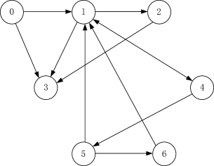
Figure 1: The leader-follower directed communication graph.

Solving the LMI (5) by using the LMI toolbox of Matlab gives a feasible solution matrix $P=\begin{bmatrix}1.7559&-0.5853\\ -0.5853&0.5853\end{bmatrix}$. Then, the feedback gain matrices of (2) are given by

$$K=\begin{bmatrix}-0.8543&-2.5628\end{bmatrix},\quad\Gamma=\begin{bmatrix}0.7298&2.1893\\ 2.1893&6.5678\end{bmatrix}.$$

Let $c_{i}(0)=1$, $i=1,\cdots,6$. The consensus errors $x_{i}-x_{0}$, $i=1,\cdots,6,$ of the second-order integrators under the adaptive protocol (2) are depicted in Fig. 2 and the adaptive coupling weights $c_{i}$ are shown in Fig. 3.

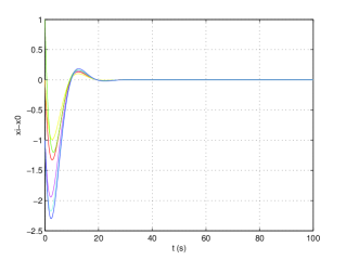
Figure 2: The consensus errors $x_{i}-x_{0}$, $i=1,\cdots,6$.

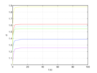
Figure 3: The adaptive coupling weights $c_{i}$.

Further, consider the case where the second-order integrators are perturbed by external disturbances. For illustration, the disturbances associated with the agents are assumed to be $\omega_{0}=\left[\begin{array}[]{c}0.1\sin(2t)\\ 0.3\sin(4t)\end{array}\right]$, $\omega_{1}=\left[\begin{array}[]{c}0.2\sin(3.5t)\\ 0.3\cos(2.5t)\end{array}\right]$, $\omega_{2}=\left[\begin{array}[]{c}0.15\cos(4t)\\ 0.2\sin(5t)\end{array}\right]$, $\omega_{3}=\left[\begin{array}[]{c}0.3\sin(x_{32})\\ 0.6\sin(3t)\end{array}\right]$, $\omega_{4}=\left[\begin{array}[]{c}0.3e^{-2t}\\ 0.15\cos(3t)\end{array}\right]$, $\omega_{5}=\left[\begin{array}[]{c}0.2\sin(4t)\\ 0.25\cos(3t)\end{array}\right]$, $\omega_{6}=\left[\begin{array}[]{c}0.3\sin(5t)\\ \frac{0.4}{x_{61}^{2}+1}\end{array}\right]$, and the control input of the leader is assumed to be $u_{0}=e^{-0.1t}$. Solving the LMI (17) with $\varepsilon=2$ gives $Q=\begin{bmatrix}0.2622&-0.3517\\ -0.3517&0.7395\end{bmatrix}$ and then $K=\begin{bmatrix}-5.0141&-3.7372\end{bmatrix}$, $\Gamma=\begin{bmatrix}25.1412&18.7386\\ 18.7386&13.9665\end{bmatrix}$. In (14), let $\varphi_{i}=0.1$ and $d_{i}(0)=1.5$, $i=1,\cdots,6$. The consensus errors $x_{i}-x_{0}$, $i=1,\cdots,6,$ under the robust adaptive protocol (14) are depicted in Fig.4 and the coupling weights $d_{i}$ are shown in Fig. 5, both of which are obviously bounded.

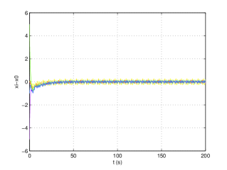
Figure 4: The consensus errors under the robust adaptive protocol (14).

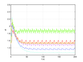
Figure 5: The coupling weights $d_{i}$ in the presence of disturbances.

6 Conclusion

In this paper, we have presented novel distributed adaptive consensus protocols for linear multi-agent systems with external disturbances and directed graphs containing a directed spanning tree with the leader as the root. The adaptive consensus protocols, depending on only the agent dynamics an the relative state information of neighboring agents, can be designed and implemented in a fully distributed way. One contribution of this paper is that the new distributed adaptive protocol is robust in the presence of general bounded external disturbances. An interesting topic for future investigation is to design fully distributed adaptive protocols for nonlinear multi-agent systems or the case with local output information of each agent and its neighbors.

References

• [1] W. Ren, R. Beard, and E. Atkins (2007). Information consensus in multivehicle cooperative control. IEEE Control Systems Magazine vol. 27 no. 2 (71–82).
• [2] Y. Hong, G. Chen, and L. Bushnell (2008). Distributed observers design for leader-following control of multi-agent networks. Automatica vol. 44 no. 3 (846–850).
• [3] R. Olfati-Saber and R. Murray (2004). Consensus problems in networks of agents with switching topology and time-delays. IEEE Transactions on Automatic Control vol. 49 no. 9 (1520–1533).
• [4] T. Li, M. Fu, L. Xie, and J. Zhang (2011). Distributed consensus with limited communication data rate. IEEE Transactions on Automatic Control vol. 56 no. 2 (279–292).
• [5] Z. Li, Z. Duan, and G. Chen (2011). On $H_{\infty}$ and $H_{2}$ performance regions of multi-agent systems. Automatica vol. 47 no. 4 (797–803).
• [6] M. Guo and D. V. Dimarogonas (2013). Consensus with quantized relative state measurements. Automatica vol. 49 no. 8 (2531–2537).
• [7] Z. Li, Z. Duan, G. Chen, and L. Huang (2010). Consensus of multiagent systems and synchronization of complex networks: A unified viewpoint. IEEE Transactions on Circuits and Systems I: Regular Papers vol. 57 no. 1 (213–224).
• [8] Z. Li, Z. Duan, and G. Chen (2011). Dynamic consensus of linear multi-agent systems. IET Control Theory and Applications vol. 5 no. 1 (19–28).
• [9] S. Tuna (2009). Conditions for synchronizability in arrays of coupled linear systems. IEEE Transactions on Automatic Control vol. 54 no. 10 (2416–2420).
• [10] J. Seo, H. Shim, and J. Back (2009). Consensus of high-order linear systems using dynamic output feedback compensator: Low gain approach. Automatica vol. 45 no. 11 (2659–2664).
• [11] H. Zhang, F. Lewis, and A. Das (2011). Optimal design for synchronization of cooperative systems: State feedback, observer, and output feedback. IEEE Transactions on Automatic Control vol. 56 no. 8 (1948–1952).
• [12] C. Ma and J. Zhang (2010). Necessary and sufficient conditions for consensusability of linear multi-sgent systems. IEEE Transactions on Automatic Control vol. 55 no. 5 (1263–1268).
• [13] Z. Li, W. Ren, X. Liu, and L. Xie (2013). Distributed consensus of linear multi-agent systems with adaptive dynamic protocols. Automatica vol. 49 no. 7 (1986–1995).
• [14] Z. Li, W. Ren, X. Liu, and M. Fu (2013). Consensus of multi-agent systems with general linear and Lipschitz nonlinear dynamics using distributed adaptive protocols. IEEE Transactions on Automatic Control vol. 58 no. 7 (1786–1791).
• [15] H. Su, G. Chen, X. Wang, and Z. Lin (2011). Adaptive second-order consensus of networked mobile agents with nonlinear dynamics. Automatica vol. 47 no. 2 (368–375).
• [16] W. Yu, W. Ren, W. X. Zheng, G. Chen, and J. Lv (2013). Distributed control gains design for consensus in multi-agent systems with second-order nonlinear dynamics. Automatica vol. 49 no. 7 (2107–2115).
• [17] Z. Li, G. Wen, Z. Duan, and W. Ren (2014). Designing fully distributed consensus protocols for linear multi-agent systems with directed communication graphs. IEEE Transactions on Automatic Control, contionally accepted.
• [18] P. A. Ioannou and J. Sun (1996). Robust Adaptive Control. New York NY: Prentice-Hall, Inc..
• [19] Z. Li, Z. Duan (2014). Distributed robust adaptive consensus protocols for linear multi-agent systems with directed graphs and external disturbances. The 2014 Chinese Control Conference, in press.
• [20] W. Ren and R. Beard (2005). Consensus seeking in multiagent systems under dynamically changing interaction topologies. IEEE Transactions on Automatic Control vol. 50 no. 5 (655–661).
• [21] Z. Qu (2009). Cooperative Control of Dynamical Systems: Applications to Autonomous Vehicles. London, UK: Spinger-Verlag.
• [22] H. Zhang, F. L. Lewis, and Z. Qu (2012). Lyapunov, adaptive, and optimal design techniques for cooperative systems on directed communication graphs. IEEE Transactions on Industrial Electronics vol. 59 no. 7 (3026–3041).
• [23] D. S. Bernstein (2009). Matrix Mathematics: Theory, Facts, and Formulas. Princeton University Press.
• [24] M. Corless and G. Leitmann (1981). Continuous state feedback guaranteeing uniform ultimate boundedness for uncertain dynamic systems. IEEE Transactions on Automatic Control vol. 26 no. 5 (1139–1144).
• [25] M. Krsti c, I. Kanellakopoulos, and P. Kokotovic (1995). Nonlinear and Adaptive Control Design. New York: John Wiley Sons.