The HLS approach to $(g-2)_{\mu}$ : A Solution to the “$\tau$ versus $e^{+}e^{-}$” Puzzle

Abstract

The Hidden Local Symmetry (HLS) Model provides a framework able to encompass several physical processes and gives a unfied description of these in an energy range extending up to the $\phi$ mass. Supplied with appropriate symmetry breaking schemes, the HLS Model gives a broken Effective Lagrangian (BHLS). The BHLS Lagrangian gives rise to a fit procedure in which a simultaneous description of the $e^{+}e^{-}$ annihilations to $\pi^{+}\pi^{-}$, $\pi^{0}\gamma$, $\eta\gamma$, $\pi^{+}\pi^{-}\pi^{0}$, $K^{+}K^{-}$, $K_{L}K_{S}$ and of the dipion spectrum in the decay $\tau^{\pm}\rightarrow\pi^{\pm}\pi^{0}\nu$ can be performed. Supplemented with a few pieces of information on the $\rho^{0}-\omega-\phi$ system, the $\tau$ dipion spectrum is shown to predict accurately the pion form factor in $e^{+}e^{-}$ annihilations. Physics results derived from global fits involving or excluding the $\tau$ dipion spectra are found consistent with each others. Therefore, no obvious mismatch between the $\tau$ and $e^{+}e^{-}$ physics properties arises and the $\tau-e^{+}e^{-}$ puzzle vanishes within the broken HLS Model.

1 Introduction

The pion form factor in the $e^{+}e^{-}\rightarrow\pi^{+}\pi^{-}$ annihilation ($F_{\pi}^{ee}(s)$) and in the the $\tau^{\pm}\rightarrow\pi^{\pm}\pi^{0}\nu$ decay ($F_{\pi}^{\tau}(s)$) are expected to differ only by isospin symmetry breaking (IB) terms. Understanding the relationship between $F_{\pi}^{ee}(s)$ and $F_{\pi}^{\tau}(s)$ is important as it can allow for 2 different evaluations of the dipion contribution to $a_{\mu}(\pi\pi)$, the muon Hadronic Vacuum Polarization (HVP) which could be merged together if consistent with each other. However, this relationship supposes a good understanding of isospin symmetry breaking and an appropriate modelling.

For a long time puzzle1 ; puzzle2 , the comparison between $|F_{\pi}^{ee}(s)|^{2}$ and $|F_{\pi}^{\tau}(s)|^{2}$ was not satisfactory and the mismatch Davier2007 was severe enough that one started to speak of a "$e^{+}e^{-}$ vs $\tau$" puzzle. This has continued up to very recently DavierHoecker3 . However, some works taupaper ; Fred11 indicated that this puzzle could well be a modelling issue of the isospin symmetry breaking phenomenon. On the other hand, it was also shown DavierHoecker that, numerically, the $e^{+}e^{-}-\tau$ discrepancy sensitively depends on the $e^{+}e^{-}\rightarrow\pi^{+}\pi^{-}$ sample considered. Therefore the so–called $e^{+}e^{-}-\tau$ puzzle may carry several components.

The Hidden Local Symmetry (HLS) Model provides a framework and a procedure able to address this puzzle in the various aspects just sketched. The HLS model encompasses several physical processes and gives a unfied description of these in an energy range extending up to the $\phi$ mass. However, in order to account precisely for experimental data, it should be supplied with several symmetry breaking schemes. Among these, an energy dependent mixing mechanism of the neutral vector meson system ($\rho^{0}-\omega-\phi$) is generated via loop effects and allows to define an effective broken HLS (BHLS) model. Within this framework, the $e^{+}e^{-}$ annihilations to $\pi^{+}\pi^{-}$, $\pi^{0}\gamma$, $\eta\gamma$, $\pi^{+}\pi^{-}\pi^{0}$, $K^{+}K^{-}$, $K_{L}K_{S}$ and the dipion spectrum in the decay $\tau^{\pm}\rightarrow\pi^{\pm}\pi^{0}\nu$ are $simultaneously$ accounted for with the same set of parameters derived from global fits in procedures involving all the existing data samples covering the channels listed above. One can also define a variant – named $\tau$ + PDG – where the $e^{+}e^{-}\rightarrow\pi^{+}\pi^{-}$ data are replaced by tabulated $\rho^{0}$, $\omega$ and $\phi$ particle propertiesRPP2012 ; with such a tool, one can compare the $\tau$ predictions for the $e^{+}e^{-}\rightarrow\pi^{+}\pi^{-}$ annihilation and the data. If the $e^{+}e^{-}-\tau$ puzzle is a relevant concept, this comparison should enhance the issue.

After a brief review of the BHLS Model and its breaking in Sections 2, 3 and 4, the various aspects of the global fit method are outlined in Section 5. Section 6 studies the $\tau$ +PDG predictions and their comparison with the existing $e^{+}e^{-}\rightarrow\pi^{+}\pi^{-}$ data samples. In Section 7, one reports on global fits mixing $e^{+}e^{-}\rightarrow\pi^{+}\pi^{-}$ and $\tau$ dipion data. In Section 8, the effects of $\tau$ data on the muon HVP are displayed. Section 9 is devoted to conclusions.

2 Basics of the Hidden Local Symmetry Model

The Hidden Local Symmetry Model (HLS) Model is a framework which encompasses simultaneously several different physics processes covered by a large number of already available data samples. A comprehensive review of the HLS Model is given in HLSRef and a brief account can be found in ExtMod3 ; however, in order to really deal with experimental data at their present level of accurate, breaking procedures need to be implemented. As these are tightly connected with the HLS Model structure, it is worth giving a brief outline of its main features.

Beside its non–anomalous sector, which allows to address some $e^{+}e^{-}$ annihilation channels and some $\tau$ decays, the HLS Model also contains an anomalous (FKTUY) sector FKTUY ; HLSRef which provides couplings of the form $VVP$, $VPPP$, $\gamma PPP$,$VP\gamma$ or $P\gamma\gamma$ among the light flavor mesons. Intrisically, the HLS validity range does not extend much beyond the $\phi$ mass.

If the $e^{+}e^{-}\rightarrow\pi^{+}\pi^{-}/K\overline{K}$ annihilations or the $\tau^{\pm}\rightarrow\pi^{\pm}\pi^{0}\nu$ decay clearly proceed from the non–anomalous sector of the HLS model, decays involving, for instance, $VP\gamma$ or $P\gamma\gamma$ couplings obviously imply the anomalous HLS sectors. On the other hand, both the anomalous and non–anomalous sectors of the HLS Model are mandatorily requested to account for annihilation channels like $e^{+}e^{-}\rightarrow\pi^{0}\gamma$, $e^{+}e^{-}\rightarrow\eta\gamma$ or $e^{+}e^{-}\rightarrow\pi^{0}\pi^{+}\pi^{-}$.

The construction of the HLS Lagrangian starts by defining the (right and left) $\xi$ fields :

$$\xi_{R,L}=\displaystyle\exp{[\pm i\displaystyle P/f_{\pi}]}$$ (1)

where $f_{\pi}$ is the pion decay constant and $P=P_{8}+P_{0}$ is the U(3) matrix of the pseudoscalar fields which includes the octet and singlet field components ExtMod3 .

The HLS non–anomalous Lagrangian is defined by :

$$\left\{\begin{array}[]{lll}{\cal L}_{HLS}=&{\cal L}_{A}+a{\cal L}_{V}&\nobreak\leavevmode\nobreak\leavevmode\\[8.5359pt] {\cal L}_{A}=&\displaystyle-\frac{f_{\pi}^{2}}{4}{\rm Tr}[(D_{\mu}\xi_{L}\xi_{L}^{\dagger}-D_{\mu}\xi_{R}\xi_{R}^{\dagger})^{2}]&\displaystyle\equiv-\frac{f_{\pi}^{2}}{4}{\rm Tr}[L-R]^{2}\\[8.5359pt] {\cal L}_{V}=&\displaystyle-\frac{f_{\pi}^{2}}{4}{\rm Tr}[(D_{\mu}\xi_{L}\xi_{L}^{\dagger}+D_{\mu}\xi_{R}\xi_{R}^{\dagger})^{2}]&\displaystyle\equiv-\frac{f_{\pi}^{2}}{4}{\rm Tr}[L+R]^{2}\\[8.5359pt] \end{array}\right.$$ (2)

These expressions involve the covariant derivatives of the $\xi_{R,L}$ fields :

$$\left\{\begin{array}[]{ccc}D_{\mu}\xi_{L}=\displaystyle\partial_{\mu}\xi_{L}-igV_{\mu}\xi_{L}+i\xi_{L}{\cal L}_{\mu}\\[8.5359pt] D_{\mu}\xi_{R}=\displaystyle\partial_{\mu}\xi_{R}-igV_{\mu}\xi_{R}+i\xi_{R}{\cal R}_{\mu}\end{array}\right.$$ (3)

which introduce the usual bare vector field matrix $V$; the other gauge bosons of the Standard Model ($A$, $W^{\pm}$ and $Z$) are hidden inside ${\cal L}_{\mu}$ and ${\cal R}_{\mu}$; neglecting the influence of the $Z$ boson field absent from the physics we address, these write :

$$\left\{\begin{array}[]{l}{\cal L}_{\mu}=\displaystyle eQA_{\mu}+\frac{g_{2}}{\sqrt{2}}(W^{+}_{\mu}T_{+}+W^{-}_{\mu}T_{-})\\[8.5359pt] {\cal R}_{\mu}=\displaystyle eQA_{\mu}\end{array}\right.$$ (4)

The quark charge matrix $Q$ is standard and the matrix $T_{+}=[T_{-}]^{\dagger}$ is constructed out of matrix elements of the Cabibbo–Kobayashi–Maskawa matrix HLSRef . Concerning the physics parameters, the above expressions exhibit the electric charge $e$, the universal vector coupling $g$ and the weak coupling $g_{2}$ (related with the Fermi constant by $g_{2}=2m_{W}\sqrt{G_{F}\sqrt{2}}$). Finally, $a$ is a specific HLS parameter not fixed by the model and expected of the order 2.

3 Usual symmetry breaking schemes of the HLS Model

The HLS model obviously provides an elegant unified framework which covers an important set of annihilation and decay processes. However, as such, it cannot produce a satisfactory account of the real experimental data falling into its scope. A simple illustration is given by the pion and kaon decay constants found of equal magnitudes within the unbroken HLS Lagrangian.

This clearly indicates that symmetry breaking mechanisms should be supplied. The authors of the HLS Model were aware of this difficulty and soon proposed a simple (BKY) mechanism to break the flavor SU(3) symmetry BKY of the model; this has been later extended to include isospin breaking Hashimoto ; for practical purpose, we use the BKY mechanism as reformulated in Heath . Within the non–anomalous HLS Lagrangian pieces, the BKY mechanism turns out to perform the substitutions :

$$\left\{\begin{array}[]{ccc}{\cal L}_{A}::&\displaystyle-\frac{f_{\pi}^{2}}{4}{\rm Tr}[(L-R)]^{2}\Rightarrow-\frac{f_{\pi}^{2}}{4}{\rm Tr}[(L-R)X_{A}]^{2}\\[8.5359pt] {\cal L}_{V}::&\displaystyle-\frac{f_{\pi}^{2}}{4}{\rm Tr}[(L+R)]^{2}\Rightarrow\equiv-\frac{f_{\pi}^{2}}{4}{\rm Tr}[(L+R)X_{V}]^{2}\end{array}\right.$$ (5)

where $X_{A}$ and $X_{V}$ are real diagonal matrices :

$$\left\{\begin{array}[]{ll}\displaystyle X_{A}=&{\rm Diag}(q_{A},y_{A},z_{A})\\[8.5359pt] \displaystyle X_{V}=&{\rm Diag}(q_{V},y_{V},z_{V})\leavevmode\nobreak\ \leavevmode\nobreak\ \leavevmode\nobreak\ \leavevmode\nobreak\ \leavevmode\nobreak\ .\end{array}\right.$$ (6)

which should be derived from data.

The departures of $q_{A/V}$ and $y_{A/V}$ from 1 measure the isospin symmetry breaking, while $z_{A/V}$ carry the flavor SU(3) symmetry breaking. Together with determinant terms tHooft which permit to break nonet symmetry in the pseudoscalar sector, this provides a reliable description of the light meson radiative decays and of the $e^{+}e^{-}\rightarrow P\gamma$ annihilations.

4 Vector field mixing, a new symmetry breaking mechanism

The coupling of the neutral vector mesons carrying no open strangeness to a pseudoscalar meson pair is given by the following piece of the ${\cal L}_{V}$ HLS Lagrangian taupaper  :

$$\begin{array}[]{ll}\nobreak\leavevmode\nobreak\leavevmode&\displaystyle\frac{iag}{2}\rho^{0}_{I}\pi^{-}\stackrel{{\scriptstyle\leftrightarrow}}{{\partial}}\pi^{+}+\frac{iag}{4z_{A}}(\rho^{0}_{I}+\omega_{I}-\sqrt{2}z_{V}\phi_{I})K^{-}\stackrel{{\scriptstyle\leftrightarrow}}{{\partial}}K^{+}\\ \nobreak\leavevmode\nobreak\leavevmode&+\displaystyle\frac{iag}{4z_{A}}(\rho^{0}_{I}-\omega_{I}+\sqrt{2}z_{V}\phi_{I})K^{0}\stackrel{{\scriptstyle\leftrightarrow}}{{\partial}}\overline{K}^{0}\end{array}$$ (7)

The last two terms obviously give rise to pseudoscalar kaon loops which modify the vector mass matrix by $s$–dependent terms. Moreover, the kaon loops generate transitions among the ideal $\rho_{I}$, $\omega_{I}$ and $\phi_{I}$ of the original Lagrangian and, thus, give $non-diagonal$ entries inside the vector meson squared mass matrix taupaper ; ExtMod3 . Stated otherwise, at one–loop order, the ideal $\rho_{I}$, $\omega_{I}$ and $\phi_{I}$ fields are no longer mass eigenstates as expected for the physical vector meson fields. The one–loop order mass squared matrix writes :

$$\left\{\begin{array}[]{lll}\displaystyle M^{2}(s)&=M^{2}_{0}(s)+\delta M^{2}(s)\leavevmode\nobreak\ \leavevmode\nobreak\ \leavevmode\nobreak\ \leavevmode\nobreak\ {\rm with\leavevmode\nobreak\ :}\\ \displaystyle M^{2}_{0}(s)&={\rm Diag}(m^{2}+\Pi_{\pi\pi}(s),\leavevmode\nobreak\ m^{2},\leavevmode\nobreak\ z_{V}m^{2}).\end{array}\right.$$ (8)

where $\delta M^{2}(s)$ is a non–diagonal perturbation matrix depending on the kaon loops to the (otherwise) diagonal matrix $M^{2}_{0}(s)$. The entries of $M^{2}_{0}(s)$ depend on $m^{2}$ – the squared $\rho$ (or $\omega$) meson mass, as it occurs in the original HLS Lagrangian – and on $\Pi_{\pi\pi}(s)$, the dipion loop to which only $\rho_{I}$ couples.

As $\delta M^{2}(s)$ is small compared to $M^{2}_{0}(s)$ within the range of validity of the HLS model (i.e. up to the $\phi$ mass region), the eigenvalue problem Eq. (8) can be solved perturbatively. The relation between the ideal fields ($V_{I}$) and the physical fields ($V_{R}$) can be written :

$$\left(\begin{array}[]{lll}\rho_{I}\\[8.5359pt] \omega_{I}\\[8.5359pt] \phi_{I}\end{array}\right)=\left(\begin{array}[]{cll}\displaystyle 1&-\alpha&\beta\\[8.5359pt] \displaystyle\alpha&1&\gamma\\[8.5359pt] \displaystyle-\beta&-\gamma&1\end{array}\right)\left(\begin{array}[]{cll}\rho^{0}_{R}\\[8.5359pt] \omega_{R}\\[8.5359pt] \phi_{R}\end{array}\right)$$ (9)

where $\alpha$, $\beta$ and $\gamma$ are functions of $s$, the energy flowing through the vector meson line. These functions essentially depend on the sum and the difference of the charged and neutral kaon loops and are small compared to 1 taupaper ; ExtMod3 . Therefore, the vector field mixing mechanism introduces breaking terms which are $s$–dependent, $s$ being the running vector meson mass.

Figure 1: The ratio $f_{\rho^{0}\gamma}(s)/f_{\rho^{\pm}W}$ derived from a BHLS global fit over the region from the two–pion threshold to slightly above the $\phi$ mass

.

This change of fields is what mostly generates an isospin 1 component inside the physical $\omega$ and $\phi$ mesons and, then, their couplings to a pion pair as, using Eq. (9), one gets at first order in breaking parameters :

$$\begin{array}[]{ll}\nobreak\leavevmode\nobreak\leavevmode&\displaystyle\frac{iag}{2}\rho_{I}\leavevmode\nobreak\ \cdot\leavevmode\nobreak\ \pi^{-}\stackrel{{\scriptstyle\leftrightarrow}}{{\partial}}\pi^{+}\Rightarrow\\ \nobreak\leavevmode\nobreak\leavevmode&\displaystyle\frac{iag(1+\Sigma_{V})}{2}\left[\rho^{0}_{R}+[(1-h_{V})\Delta_{V}-\alpha(s)\omega+\beta(s)\phi\right]\cdot\leavevmode\nobreak\ \pi^{-}\stackrel{{\scriptstyle\leftrightarrow}}{{\partial}}\pi^{+}\end{array}$$ (10)

At this order, the $\rho^{0}_{R}$ coupling to a pion pair is unchanged and remains identical to those of the $\rho^{\pm}$ meson. On the other hand, the change of fields Eq. (9) modifies the Lagrangian coupling of the neutral $\rho$ meson to the photon, while leaving unchanged the charged $\rho$ coupling to the $W$ boson. Therefore, the vector field mixing makes the ratio of these two couplings $s$–dependent :

$$\frac{f_{\rho^{0}\gamma}(s)}{f_{\rho^{\pm}W}}=\left[1+\frac{h_{V}\Delta_{V}}{3}+\frac{\alpha(s)}{3}+\frac{\sqrt{2}z_{V}}{3}\beta(s)\right]\leavevmode\nobreak\ \leavevmode\nobreak\ .$$ (11)

In order to substantiate this specific breaking of the HLS model, let us quote a result derived from a global fit involving all the channels listed in the Introduction; the ratio $f_{\rho^{0}\gamma(s)}/f_{\rho^{\pm}W}$ shown in Figure 1 exhibits significant variations over the HLS energy range of interest. It is the main mechanism which allows to reconcile the $\tau$ dipion spectrum and the $e^{+}e^{-}\rightarrow\pi^{+}\pi^{-}$ annihilation cross section. These couplings are supplemented by loop corrections taupaper ; ExtMod3 which also play an important role in defining the effective $\gamma V$ mixings.

On the other hand, the $\tau$ decay process also undergoes several specific breaking effects : The short range Marciano and long range Cirigliano corrections are included when fitting the $\tau$ dipion spectrum, as for the specific $\pi^{\pm}\pi^{0}$ phase space factor. These $\tau$ breaking effects are accounted for within fits as usually done; they are clearly independent of the HLS breaking mechanisms and only come supplementing them.

5 The various aspects of the global fit method

Gradually equipped since taupaper with the various breaking procedures briefly outlined above, the HLS Model has evolved toward a broken version (BHLS) ExtMod3 able now to cope simultaneously with several physics processes, namely the $e^{+}e^{-}$ annihilations to $\pi^{+}\pi^{-}$, $\pi^{0}\gamma$, $\eta\gamma$, $\pi^{+}\pi^{-}\pi^{0}$, $K^{+}K^{-}$, $K_{L}K_{S}$, the dipion spectrum in the decay $\tau^{\pm}\rightarrow\pi^{\pm}\pi^{0}\nu$ and, additionally, some more radiative decays of light flavor mesons. It involves 25 parameters to be extracted from data which come intricated simultaneously within the various amplitudes.

Therefore, BHLS is a global model and permits a global fit of the processes just listed. As each of the model parameters is involved in several processes, this gives rise to $physics$ correlations among the various processes belonging to the BHLS realm. This also propagates to correlating the data samples covering any of the channels involved. One obviously expects herefrom an improvement of the uncertainties as, for each channel, the available experimental statistics is practically enhanced by the data collected in any of the other channels covered by BHLS. Of course, the fit quality is expected to reflect that these physics constraints are well accepted by the data.

The number of independent data samples covering the various quoted channels is of the order 50; they are listed and discussed in ExtMod3 . In this Reference, a simultaneous fit of all available $e^{+}e^{-}$ annihilation scan data and of the published $\tau$ dipion spectra is performed. A very good fit quality is reached and no noticeable issue is observed. As the model is global, it also represents a new tool to examine precisely several issues ExtMod4  :

1. The discrepancy between the dipion spectrum in the $\tau$ decay and in the $e^{+}e^{-}$ annihilation,

2. The relative compatibility of the various available $e^{+}e^{-}\rightarrow\pi^{+}\pi^{-}$ cross section measurements up to the $\phi$ mass,

3. The compatibility of the $\tau$ and $e^{+}e^{-}$ based estimates of the hadronic vacuum polarization (HVP) contribution to the muon $g-2$.

The following sections outline the BHLS analysis of these issues.

6 The BHLS prediction of the pion form factor in $e^{+}e^{-}$ annihilations

Since 2002 several measurements of the pion form factor in $e^{+}e^{-}$ annihilations have been published. Beside the data samples collected in scan mode by CMD–2 CMD-2 and SND SND , the KLOE Collaboration has produced three spectra collected in the ISR mode under different conditions, namely KLOE08 KLOE08 , KLOE10 KLOE10 and recently the KLOE12 data sample KLOE12 – strongly correlated with KLOE08. BaBar has also produced a $\pi^{+}\pi^{-}$ spectrum BaBar extending up to 1.8 GeV. Finally, very recently, the BESS III Collaboration has published a new spectrum BESS-III limited to the energy interval $0.6-0.9$ GeV. Except for the BESS data sample presented in ExtMod5 , these data samples have been examined in either of ExtMod4 or Conf_2013 – specifically for the KLOE12 sample. The present study outlines the treatment of the BESS III sample within the BHLS fitter.

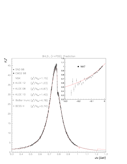
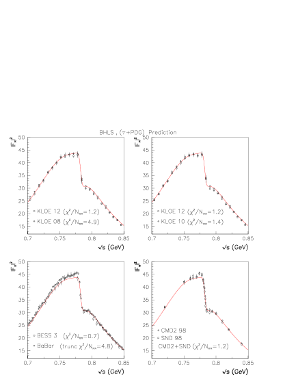
Figure 2: Predictions for the pion form factor in the $e^{+}e^{-}\to\pi^{+}\pi^{-}$ annihilation derived using the $\tau$ + PDG method. None of the $\pi^{+}\pi^{-}$ spectra is used in the fitting procedure. The leftmost pannel displays the overall picture with data superimposed, the inset showing the form factor continuation into the spacelike ($s<0$) region. The rightmost pannel displays, enlarged, the behavior of the various data samples in the $\rho-\omega$ interference region.

A priori, BHLS can predict the pion form factor in the $e^{+}e^{-}\to\pi^{+}\pi^{-}$ annihilation relying on the measured $\tau$ dipion spectra Aleph ; Cleo ; Belle , provided it is also fed with the appropriate isospin breaking (IB) information. However, despite the intricacy phenomenon noted above, some of the specific IB effects occuring in the $e^{+}e^{-}\to\pi^{+}\pi^{-}$ annihilation are marginally constrained by the other annihilation channels included within the BHLS realm. So, specific data directly reflecting these IB effects should be provided to the BHLS fitter. Such pieces of information are obviously related with the $\omega/\phi\to\pi^{+}\pi^{-}$ couplings. Reference ExtMod4 proposed to use the corresponding tabulated RPP2012 partial widths and the (Orsay) phases between the $\omega/\phi$ amplitudes and the underlying coherent $\pi^{+}\pi^{-}$ background; this phase information can be replaced by the relevant tabulated products $\Gamma(V\rightarrow e^{+}e^{-})\times\Gamma(V\rightarrow\pi^{+}\pi^{-})$. Additionally, as the $\rho^{0}\to e^{+}e^{-}$ coupling is marginally constrained by the non–$\pi^{+}\pi^{-}$ annihilation data, one should include the tabulated $\rho^{0}\to e^{+}e^{-}$ decay width. This method is named $\tau$ +PDG for obvious reasons.

For reasons which will become clear soon, it deserves noting that none of the 5 pieces of information supplementing the $\tau$ spectra in the $\tau$+PDG approach is influenced by any of the KLOE, BaBar or BESS III $\pi^{+}\pi^{-}$ spectra. Actually, they are almost 100% determined by the data collected by the CMD–2 and SND Collaborations.

The red curve in Figure 2 displays the $\tau$ +PDG distribution and, superimposed, all the available $e^{+}e^{-}\to\pi^{+}\pi^{-}$ data samples. When minuit has converged, one can compute the $\chi^{2}$ distance of each of the available $\pi^{+}\pi^{-}$ spectra to the $\tau$ +PDG best fit function; the average $\chi^{2}$ per data point is then calculated for each data sample and all are reported inside the plots as comments.

Obviously, the left–hand side pannel indicates that, overall, the agreement between the $\tau$ +PDG $prediction$ and the data is satisfactory, and the inset indicates that this agreement extends to the close spacelike region. Therefore, the accepted (PDG) values for the IB pieces of information listed above allow to recover the gross features of the pion form factor with a noticeable precision; this already indicates that the IB mechanism as plugged within BHLS is appropriate.

The right–hand side pannel, however, indicates that we are faced with a contrasting picture, depending on the data samples examined. As a good tag of the agreement between the BHLS $\tau$ +PDG and the (secure) NSK data, the relevant subpannel in the right–hand side of Figure 2 displays the average $\chi^{2}$ distance per data point of the NSK samples; one gets $\overline{\chi}^{2}_{NSK}=1.2$, close to the best fit value in a fit where the PDG information is replaced by the CMD–2 and SND $e^{+}e^{-}\to\pi^{+}\pi^{-}$ data samples ExtMod3 . This also gives a hint about the range of acceptable values for the $\overline{\chi}^{2}$ associated with any given sample.

Therefore, the BHLS fit in the $\tau$+PDG mode provides IB parameter values which allow the underlying (BHLS) IB framework to exhibit a full consistency of all non $\pi^{+}\pi^{-}$ data with the $\pi^{+}\pi^{-}$ NSK (i.e. CMD–2 & SND) data. The picture is clearly alike for the KLOE10 ($\overline{\chi}^{2}_{KLOE10}=1.4$), KLOE12 ($\overline{\chi}^{2}_{KLOE12}=1.2$) and BESSIII ($\overline{\chi}^{2}_{BESS}=0.7$) data samples. In contrast, one observes that the KLOE08 ($\overline{\chi}^{2}_{KLOE08}=4.9$) or BaBar ($\overline{\chi}^{2}_{BaBar\leavevmode\nobreak\ trunc}=4.8$) samples are farther than could be expected.

The upper left–hand plot in the right pannel of Figure 2 is also quite informative; indeed it shows that the twin samples KLOE08 and KLOE12 KLOE08 ; KLOE12 carry central values very close to each other and that both follow almost exactly the $\tau$ +PDG predicted curve. Nevertheless, KLOE12 exhibits a $\overline{\chi}^{2}$ value in close agreement with the $\tau$ +PDG expectations while KLOE08 does not. This should be due to the estimates and structure of the reported correlated systematic uncertainties, seemingly better understood for the KLOE12 sample.

Finally, there is a clear contradiction between the KLOE and BaBar samples, as already reported by other authors (see for instance DavierHoecker ) but, also, BaBar does not fit well with the BHLS $\tau$ +PDG predictions.

Therefore, as in the comparison between the $\tau$ +PDG predictions and the various $\pi^{+}\pi^{-}$ data samples, five out of the seven available independent $\pi^{+}\pi^{-}$ samples do not exhibit any kind of mismatch, one is obviously tempted to conclude that there is no evidence for a $\tau-e^{+}e^{-}$ puzzle. The BHLS approach would rather indicate that the reported puzzle comes from a non–adequate IB modelling.

Table 1: Fit mixing the indicated $e^{+}e^{-}\to\pi^{+}\pi^{-}$ samples $and$ the $\tau$ spectra in single mode or combined. The values are the ratios $\chi^{2}/N_{\pi^{+}\pi^{-}}$ returned by the fits and the global fit probability are given for each data sample or for the selected sample combinations.

Fit Cond.	KLOE08	KLOE10	KLOE12	NSK	BESS	BaBaR	BaBaR
$\chi^{2}/N_{\pi^{+}\pi^{-}}$						(trunc)	(full)
Single	1.64	0.96	1.02	0.96	0.56	1.15	1.25
(prob)	(59%)	(97%)	(97%)	(97%)	(99%)	(74%)	(40%)
Comb. 1 (0.98 [99%])	$-$	1.00	1.05	1.11	0.61	$-$	$-$
Comb. 2 (1.06 [97%])	$-$	1.02	1.05	1.10	$-$	$-$	$-$
Comb. 3 (1.21 [22%])	$-$	1.01	1.54	1.18	0.56	$1.36$	$-$

7 The BHLS global fits

So, the comparison between the $\tau$ predictions – also based on commonly accepted PDG information – and the various $\pi^{+}\pi^{-}$ data samples indicates various behaviors. More precisely, the $\tau$ + PDG method gives a well–founded indication that the CMD–2, SND, KLOE10, KLOE12 and BESSIII $e^{+}e^{-}\to\pi^{+}\pi^{-}$ data samples should be quite consistent with the $\tau$ dipion spectra; in contrast, one may expect that KLOE08 and BaBar should exhibit some difficulty to accomodate the $\tau$ spectra within the BHLS framework. A step further is to perform global fits within the BHLS framework including the $\tau$ spectra and the various $e^{+}e^{-}\to\pi^{+}\pi^{-}$ data samples, each in isolation or in combinations. The results obtained should allow for more conclusive statements.

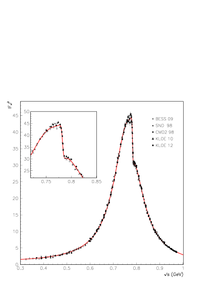
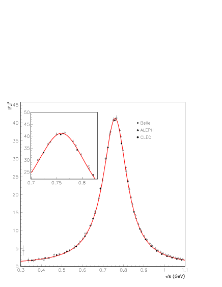
Figure 3: The pion form factor in the $e^{+}e^{-}\to\pi^{+}\pi^{-}$ annihilation (left–hand pannel) and in the $\tau$ decay (right–hand pannel) derived from a BHLS fit involving the CMD–2, SND, KLOE10, KLOE12 and BESS data samples, on the one hand, and the ALEPH, CLEO and Belle dipion spectra, on the other hand.

The first data line in Table 1 reports some fit information derived using the various $\pi^{+}\pi^{-}$ samples in isolation, namely their various $\overline{\chi}^{2}$ and their global fit probabilities; in these fits, the PDG information previously referred to should be removed. One observes a significant gap between KLOE08 and BaBar, on the one hand and the five other data samples, on the other hand.

In the same Table, one also displays the fit results associated with different combinations of the existing data samples. This Table shows that the largest set where each data sample has an average $\chi^{2}$ per point close to its value in its single mode fit is Combination 1; this combination is our reference for the following. For this combination, the $\overline{\chi}^{2}$ of the whole set of $\pi^{+}\pi^{-}$ data sample is 0.98 with an associated large probability as indicated in the first column.

The pion form factor (FF) in $e^{+}e^{-}$ annihilations and in the $\tau$ decay derived from fitting with Combination 1 are displayed in Figure 3; they are clearly satisfactory. The older $\pi^{+}\pi^{-}$ data reported in Barkov are also included in the fit and, on the whole, one yields $\chi^{2}_{\pi^{+}\pi^{-}}/N_{\pi^{+}\pi^{-}}=361.5/404$ and $\chi^{2}_{\pi^{\pm}\pi^{0}}/N_{\pi^{\pm}\pi^{0}}=86.8/85$. Therefore the picture looks satisfactory and this should be reflected by the residual plots.

Figure 4 displays the $e^{+}e^{-}$ pion FF residuals appropriately corrected for the reported scale uncertainty effects as discussed in the Appendix of ExtMod4 and in ExtMod5 ; it looks reasonably flat.

The pion FF in the $\tau$ decay is flat for the CLEO and Belle spectra; the ALEPH data sample tends to exhibit a small growth starting at $\simeq 850$ MeV. However, Figure 3 in AlephCorr indicates that this distribution, thanks to a bug fix, should be scaled down just in this energy region and, then, it behaves like the others.

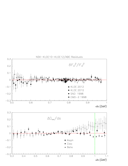
Figure 4: Residuals for the pion form factor in the $e^{+}e^{-}\to\pi^{+}\pi^{-}$ annihilation (upper pannel) and in the $\tau$ decay (lower pannel). The residuals in the upper pannel are corrected for the global scale uncertainty effects (see ExtMod4 ; ExtMod5 ).

Therefore, the global fits mixing the $\tau$ spectra and the $e^{+}e^{-}\to\pi^{+}\pi^{-}$ data samples confirm the conclusions reached in the previous Section with the $\tau$ + PDG method. Stated otherwise, global fits do not indicate any mismatch between the $e^{+}e^{-}$ and $\tau$ spectra within BHLS.

8 Including & excluding the $\tau$ spectra : Hadronic HVP issues

Let us first examine the contributions to the muon HVP provided by the pion loop in the energy region $[0.630,0.958]$ GeV; Figure 5 displays our results. The point at top of this Figure displays the $\tau$+PDG prediction for $a_{\mu}(\pi\pi,[0.63,0.958])$. The data points in red display the corresponding information directly reconstructed from the samples provided by the indicated experiments; some combinations of these are also shown. So, one observes a quite good correspondance between the "experimental" values and the prediction derived by the $\tau$+PDG method; of course, the experimental values are not influenced at all by BHLS or the $\tau$ data.

In the same Figure, one also displays the results derived when merging the $e^{+}e^{-}\to\pi^{+}\pi^{-}$ data samples and the $\tau$ dipion spectra in the minimization procedure. The empty black symbols show the fit results derived by using the iterative method defined in ExtMod5 . The points in green are the corresponding results derived from the same fits but performed without iterating. The motivation for an iterative method are emphasized in ExtMod5 and aims at cancelling out possible biases affecting the channels dominated by samples subject to dominant global scale uncertainties

Figure 5 shows that the $\tau$+PDG prediction as well as the fits merging $\tau$ and $e^{+}e^{-}$ data are consistent with each others and also with the experimental data, except for BaBar which has difficulties to accomodate the BHLS framework as shown in Table 1. Because of the energy boundaries of its spectrum, a BESSIII experimental datum for $a_{\mu}(\pi\pi,[0.63,0.958])$ cannot be produced.

Let us go a step further and examine the contributions to the muon HVP accessible through the BHLS Lagrangian and fitter which is, as already stated, limited upward slightly above the $\phi$ mass; we chose 1.05 GeV. The results are displayed in Table 2. The numbers have been derived using the iterated fit method already referred to ExtMod5 .

Let us focus on the $\pi^{+}\pi^{-}$ contribution which is actually the main aim of the present study. One thus observes that including the $\tau$ spectra shifts the central value by about $1.5\times 10^{-10}$ and improves the uncertainty by about $0.3\times 10^{-10}$ in both cases. The $1.5\times 10^{-10}$ difference between excluding and including the $\tau$ spectra looks rather small ($\simeq 1\leavevmode\nobreak\ \sigma$ or less), similar to those obtained in Fred11 , but much smaller than those in DavierHoecker3 . Therefore, within BHLS, the contribution of the $\pi^{+}\pi^{-}$ channel to the HVP does not exhibit any singular behavior : Using or not the $\tau$ spectra does not change this picture but improves the results as expected from having a larger statistics (e.g. the $\pi^{+}\pi^{-}$ $and$ the $\tau$ data).

Table 2: The various contributions to the muon HVP $a_{\mu}$ in units of $10^{-10}$ using the BHLS fit excluding the $\tau$ data (first data column), including the $\tau$ spectra (second data column), compared with the direct integration of the experimental spectra (last data column). The last line displays the total contribution accessible through the BHLS Model. The $e^{+}e^{-}$ data samples involved are those from CMD–2, SND, KLOE10, KLOE12 and BESSIII.

Channel	Excl. $\tau$	Incl. $\tau$	Direct Estim.
$\pi^{+}\pi^{-}$	$493.02\pm 1.16$	$494.59\pm 0.89$	$492.98\pm 3.38$
$\pi^{0}\gamma$	$4.50\pm 0.05$	$4.54\pm 0.04$	$3.67\pm 0.11$
$\eta\gamma$	$0.64\pm 0.01$	$0.64\pm 0.01$	$0.56\pm 0.02$
$\pi^{+}\pi^{-}\pi^{0}$	$40.84\pm 0.62$	$40.84\pm 0.57$	$43.54\pm 1.29$
$K_{L}K_{S}$	$11.53\pm 0.09$	$11.53\pm 0.08$	$12.21\pm 0.33$
$K^{+}K^{-}$	$16.88\pm 0.22$	$16.90\pm 0.20$	$17.72\pm 0.52$
Total ($<1.05$ GeV)	$567.00\pm 1.63$	$569.04\pm 1.08$	$570.68\pm 3.67$

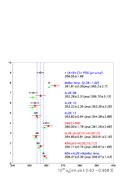
Figure 5: Values for $a_{\mu}(\pi\pi,[0.63,0.958])$ in units of 10^-10 derived from global fits using the indicated $e^{+}e^{-}\rightarrow\pi^{+}\pi^{-}$ data samples or combinations; the $\tau$ dipion spectra are always used. The full green circles are the results obtained from the $A=m$ fit (no iteration) and the black empty squares are the results obtained from the $A=M_{0}$ fit (first iteration) s explained in ExtMod5 . The values derived by directly integrating the experimental spectra are indicated by red stars. See Section 8 for comments.

9 Conclusion

The analysis developped above leads to conclude that, actually, one does not observe any mismatch between the $e^{+}e^{-}$ and the $\tau$ data. To be as precise as possible, Table 1 indicates that the $\tau$ spectra collected by ALEPH, CLEO and Belle are in perfect agreement with the CMD–2, SND, KLOE10, KLOE12 and BESSIII data samples each taken in isolation or considered together within a sample combination. This leads us to conclude that the so–called $\tau-e^{+}e^{-}$ puzzle is only due to the way the implementation of isospin symmetry breaking is performed within some models. In contrast, the BHLS approach and its way to account for IB effects seem to reflect correctly the expected relationship and the expected closeness of the $e^{+}e^{-}$ annihilation and $\tau$ decay processes. Indeed, BHLS provides successful $\tau$ predictions of the $e^{+}e^{-}$ pion form factor and a good simultaneous fit of both kinds of data.

However, we are left with a significant tension between the KLOE08 and BaBar (up to 1 GeV) samples on the one hand and the $\tau$ spectra on the other hand, as well reflected by the $\tau$+PDG information collected in Figure 2 and by the BHLS global fit results displayed in Table 1. This is indeed an issue but, seemingly, external to the so–called $\tau-e^{+}e^{-}$ puzzle which motivates this work.

References

- (1) Davier M, Eidelman S, Hoecker A and Zhang Z 2003 Eur.Phys.J. C 27 497
- (2) Davier M, Eidelman S, Hoecker A and Zhang Z 2003 Eur.Phys.J. C 31 503
- (3) Davier M 2007 Nucl. Phys. Proc. Suppl. 169 288
- (4) Davier M, Hoecker A, Malaescu B and Zhang Z 2011 Eur.Phys.J. C 71 1515 (preprint arxiv:1010.4180)
- (5) Benayoun M, David P, DelBuono L, Leitner O and O’Connell H B 2008 Eur.Phys.J. C 55 199-236 (preprint hep-ph/0711.4482)
- (6) Jegerlehner F and Szafron 2011 Eur. Phys. J. C 71 1632 (preprint arXiv:1101.2872)
- (7) Davier M, Hoecker A, Lopez Castro G, Malaescu B, Mo, X H, Toledo Sanchez G, Wang P,Yuan C Z and Zhang Z 2010 Eur. Phys. J. C 66 127–136 (preprint arxiv:0906.5443)
- (8) Harada M and Yamawaki K 2003 Phys. Rept. 381 1-233 (preprint hep-ph/0302103)
- (9) Benayoun M, David P, DelBuono, L and Jegerlehner F 2012 Eur.Phys.J. C 72 1848 (preprint arXiv:1106.1315)
- (10) Fujiwara T, Kugo T, Terao, H, Uehara S and Yamawaki K 1985 Prog. Theor. Phys. 73 926–941
- (11) Bando M, Kugo T and Yamawaki, K 1985 Nucl. Phys. B 259 493–502
- (12) Hashimoto M 1996 Phys. Rev. D 54 5611-5619
- (13) Benayoun M and O’Connell H B 1998 Phys. Rev. D 074006
- (14) ’t Hooft G 1986 Phys. Rept. 142 357-387
- (15) Marciano W J and Sirlin A 1993 Phys. Rev. Lett. 71 3629-3632
-
(16)
Cirigliano V, Ecker G and Neufeld H 2001
Phys. Lett B 513 361-370 (preprint hep-ph/0104267)
Cirigliano V, Ecker G and Neufeld H 2002 JHEP 08 002 (preprint hep-ph/027310) - (17) Benayoun M, David P, DelBuono, L and Jegerlehner F 2013 Eur.Phys.J. C 73 2453 (preprint arXiv:1210.7184)
- (18) Beringer J et al. 2012 Review of Particle Physics (RPP) Phys.Rev. D 86 010001
-
(19)
Aulchenko V M et al. 2002
Phys. Lett. B 527 161-172 (preprint hep-ex/0112031)
Akhmetshin R R et al. 2006 Phys. Lett. B 648 28-38 (preprint hep-ex/0610021)
Akhmetshin R R et al. 2006 JETP Lett. 84 413-417 (preprint hep-ex/0610016) - (20) Achasov M N et al. 2006 JJ. Exp. Theor. Phys. 103 380-384 (preprint hep-ex/0605013)
- (21) Venanzoni G et al. 2009 AIP Conf. Proc. 1182 665 (preprint arXiv:0906.4331)
- (22) Ambrosino F et al. 2011 Phys. Lett. B 700 102-110 (preprint arXiv:1006.5313)
- (23) Babusci D et al. 2013 Phys. Lett. B 720 336-343 (preprint arXiv:1212.4524)
-
(24)
Aubert B et al. 2009 Phys. Rev. Lett.
103 231801 (preprint arXiv:0908.3589)
Lees J P et al. 2012 Phys. Rev. D 86 032013 (preprint arXiv:1205.2228) - (25) Ablikim M et al. 2015 (preprint arXiv:1507.08188)
-
(26)
Benayoun M 2014 Int.J.Mod.Phys.Conf.Ser.
35 1460416
Benayoun M 2013 PoS Photon2013 048 - (27) Benayoun M, David P, DelBuono, L and Jegerlehner F 2015 (preprint arXiv:1507.02943)
- (28) Schael S et al. 2005 Phys. Rept. 421 191-284
- (29) Anderson S et al. 2000 Phys. Rev. D 61 112002 (preprint hep-ex/9910046)
- (30) Fujikawa M et al. 2008 Phys. Rev. D 78 072006 (preprint arXiv:0805.3773)
- (31) Barkov L M et al. 1985 Nucl. Phys. B 256 365-384
- (32) Davier M, Hoecker A, Malaescu B, Yuan C–Z and Zhang Z 2014 Eur.Phys.J. C 74 2803 (preprint arXiv:1312.1501)