TRIQS/DFTTools: A TRIQS application for ab initio calculations of correlated materials

Abstract

We present the TRIQS/DFTTools package, an application based on the TRIQS library that connects this toolbox to realistic materials calculations based on density functional theory (DFT). In particular, TRIQS/DFTTools together with TRIQS allows an efficient implementation of DFT plus dynamical mean-field theory (DMFT) calculations. It supplies tools and methods to construct Wannier functions and to perform the DMFT self-consistency cycle in this basis set. Post-processing tools, such as band-structure plotting or the calculation of transport properties are also implemented. The package comes with a fully charge self-consistent interface to the Wien2k band structure code, as well as a generic interface that allows to use TRIQS/DFTTools together with a large variety of DFT codes. It is distributed under the GNU General Public License (GPLv3).

PROGRAM SUMMARY

Program Title: TRIQS/DFTTools
Project homepage: https://triqs.ipht.cnrs.fr/applications/dft_tools
Catalogue identifier: –
Journal Reference: –
Operating system: Unix, Linux, OSX
Programming language: Fortran/Python
Computers: Any architecture with suitable compilers including PCs and clusters
RAM: Highly problem dependent
Distribution format: GitHub, downloadable as zip
Licensing provisions: GNU General Public License (GPLv3)
Classification: 6.5, 7.3, 7.7, 7.9
PACS: 71.10.-w,71.27.+a,71.10.Fd,71.30.+h,71.15.-m, 71.20.-b
Keywords: Many-body physics, Strongly-correlated systems, DMFT, DFT, ab initio calculations
External routines/libraries: TRIQS, cmake.
Running time: Tests take less than a minute; otherwise highly problem dependent.
Nature of problem:
Setting up state-of-the-art methods for an ab initio description of correlated systems from scratch requires a lot of code development. In order to make these calculations possible for a larger community there is need for high-level methods that allow to construct DFT+DMFT calculations in a modular and efficient way.
Solution method:
We present a Fortran/Python open-source computational library that provides high-level abstractions and modules for the combination of DFT with many-body methods, in particular the dynamical mean-field theory. It allows the user to perform fully-fledged DFT+DMFT calculations using simple and short Python scripts.

1 Introduction and Motivation

When describing the physical and also chemical properties of crystalline materials, there is a standard method that is used with great success for a large variety of systems: density functional theory (DFT). This powerful theory states that the electron density of a system uniquely determines all ground-state properties. However, in order to find the electron density in practice one usually resorts to the Kohn-Sham scheme involving an approximate exchange-correlation potential, such as the local-density or the generalized-gradient approximations. The solution of the self-consistent Kohn-Sham equations yields the Kohn-Sham orbitals (also called Bloch bands) $|\psi_{\mathbf{k}\nu}\rangle$ and the corresponding Kohn-Sham energies $\varepsilon_{\mathbf{k}\nu}$. The index $\nu$ labels the electronic band, and $\mathbf{k}$ is the wave vector within the first Brillouin zone (BZ). Below, we will always imply the Kohn-Sham scheme when talking about DFT.

The solutions of the Kohn-Sham equations form bands of allowed states in momentum space. These states are filled up to the Fermi level by the electrons according to the Pauli principle, and one can use this simple picture for example to explain the electronic band structure of materials such as elementary copper or aluminium. Following this principle one can try to classify all existing materials into metals and insulators. A system is a metal if there are an odd number of electrons per unit cell in the valence bands, since this leads to a partially filled band that cuts the Fermi energy and thus produces a Fermi surface. On the other hand, an even number of electrons per unit cell can lead to completely filled bands with a finite excitation gap to the conduction bands, i.e. insulating behaviour.

However, there are certain compounds where this classification into metals and insulators fails dramatically. This happens in particular in systems with partially filled $d$- and $f$-shells. There, DFT predicts metallic behaviour due to the open-shell setting, but in experiments many of these materials actually show insulating behaviour. This cannot be explained by band theory and the Pauli principle alone, and a different mechanism has to be invoked. The insulating behaviour in such systems, among which are the Mott insulators [1], comes by solely due to correlations between the electrons. Moreover, many interesting properties, such as transport, photoemission, etc. are temperature-dependent, which cannot be treated with a ground-state theory such as DFT alone.

In order to describe correlated materials within ab initio schemes one has to go beyond a standard DFT treatment. One step in this direction is the so called DFT+U approximation [2] which can induce the opening of a gap through a static shift of the Kohn-Sham eigenvalues. However, this technique cannot properly describe the physics of correlated metals, whose low-energy properties are dominated by dynamical many-body effects. In the mid-nineties, a very successful method was introduced to tackle this problem, namely the combination of DFT with the dynamical mean-field theory (DMFT) [3, 4, 5]. The main idea is to add local quantum correlations in the framework of DMFT to the non-local quantum Hamiltonian obtained by DFT. This method has been since applied to a large variety of problems, including high-temperature superconductors, organic insulators, iron pnictides, oxide perovskites, and other strongly-correlated materials.

Since the first proposal of DFT+DMFT, there has been a tremendous amount of new developments of numerical tools, including (fully charge self-consistent) interfaces between DFT codes and the DMFT [6, 7, 8, 9, 10, 11, 12], and exact algorithms for solving the DMFT equations [13, 14, 15, 16, 17, 18]. As a result, many more classes of materials can be studied within this framework on an ab initio basis, with much higher accuracy than just a decade ago. Importantly, these technical advances allow studies of realistic materials at experimentally interesting ambient and even lower temperatures (see, e.g., Ref. [19] for Sr₂RuO₄), in contrast to the older techniques that allowed studies down to temperatures of 1000 K only (see, e.g., Ref. [20] for the same material as above). The drawback of these new methods, however, is that they require a substantial amount of coding effort to keep up with the state-of-the-art techniques in the field.

In this paper we present version 1.3 of the TRIQS/DFTTools application, which is based on the TRIQS library [21]. The purpose of this application is to provide a complete set of tools to perform fully charge self-consistent ab initio calculations for correlated materials, and it enables researchers in the field of correlated materials to do these calculations without dedicating time to code their own implementation. The TRIQS/DFTTools package provides a fully charge self-consistent interface to the Wien2k [22] band structure program, as well as an interface that is usable with many other DFT or tight-binding codes, however, without the possibility of full charge self-consistency. Physical properties that can be calculated range from spectral functions and (projected) densities of states (DOS), charges and magnetic moments, to more involved quantities like optical conductivity and thermopower. The package can handle spin-polarised cases, as well as spin-orbit coupled systems [23]. It is released under the Free Software GPLv3 license.

The paper is organised as follows. We start with a brief general discussion of the structure of TRIQS/DFTTools in Sec. 2. In Sec. 3 we show how the interface between DFT and DMFT is set up, in particular for the Wien2k DFT package. We will also introduce the projective Wannier functions that are used as the basis set for the DMFT calculations. We continue in Sec. 4 with a simple example of a DFT+DMFT calculation, without charge self-consistency. In Sec. 5 the concept of full charge self-consistency is introduced, followed by a discussion of post-processing tools in Sec. 6. Information on how to obtain and install the code is given in Sec. 7, and we finally conclude in Sec. 8.

2 General structure of TRIQS/DFTTools

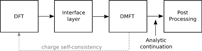
Figure 1: General structure of the TRIQS/DFTTools package.

The central part of TRIQS/DFTTools is a collection of Python modules that allow an efficient implementation of the DMFT self-consistency cycle. Since the input for this DMFT part has to be provided by DFT calculations, there needs to be another layer that connects the Python-based modules with the DFT output. Naturally, this interface depends on the DFT package at hand. Within TRIQS/DFTTools we provide an interface to the Wien2k band structure package, and a general interface that can be used in a more general setup. Note that only the Wien2k interface allows fully charge self-consistent calculations. Support for other codes is in progress.

The basic structure is schematically presented in Fig. 1. After performing a DFT calculation, the Kohn-Sham orbitals are used to construct localised Wannier orbitals, and all required information is converted into an hdf5 file. This file is used by the Python modules of TRIQS/DFTTools to perform the DMFT calculation. The fully charge self-consistent loop can be closed by taking the interacting density matrix and using it to recalculate the ground state density of the crystal in Wien2k. This leads to a new Kohn-Sham exchange-correlation potential, and thus to new orbitals. The full loop has to be repeated until convergence.

TRIQS/DFTTools also provides tools for analysing the data, such as spectral functions, densities of states, and transport properties. Depending on the method of solution of the Anderson impurity problem within the DMFT loop, the user may need to perform analytic continuation of the self-energy in order to use these tools.

3 The interface to DFT

3.1 Projective Wannier functions

In order to perform the DMFT calculations one has to choose an appropriate localised basis set. In this package, we provide a method to calculate projective Wannier functions $|w_{\mathbf{k}m}^{\alpha,\sigma}\rangle$ based on the Wien2k Kohn-Sham orbitals, as introduced in Ref. [24]. We denote orbitals in the correlated subspace $\mathcal{C}$ where many-body correlations are applied by Latin letters $m$, the index of the atom in the unit cell by $\alpha$, and the spin projection by $\sigma$.

The basic idea of the projective Wannier function technique [25] is to expand a set of local orbitals $|\chi_{m}^{\alpha,\sigma}\rangle$ over a restricted number of Bloch bands

$$|\tilde{\chi}_{\mathbf{k}m}^{\alpha,\sigma}\rangle=\sum_{\nu\in\mathcal{W}}\langle\psi_{\mathbf{k}\nu}^{\sigma}|\chi_{m}^{\alpha,\sigma}\rangle|\psi_{\mathbf{k}\nu}^{\sigma}\rangle,$$ (1)

where $\nu$ is the band index and the sum is carried out over Bloch bands within an energy window $\mathcal{W}$. Note that the functions $|\tilde{\chi}_{\mathbf{k}m}^{\alpha,\sigma}\rangle$ are not orthonormal due to this truncation.

The orbitals $\left|\tilde{\chi}_{\mathbf{k}m}^{\alpha,\sigma}\right\rangle$ can be orthonormalised, giving a set of Wannier functions:

$$\left|w_{\mathbf{k}m}^{\alpha,\sigma}\right\rangle=\sum_{\alpha^{\prime},m^{\prime}}S_{m,m^{\prime}}^{\alpha,\alpha^{\prime}}|\tilde{\chi}_{\mathbf{k}m^{\prime}}^{\alpha^{\prime},\sigma}\rangle,$$ (2)

where $S_{m,m^{\prime}}^{\alpha,\alpha^{\prime}}=\left\{O(\mathbf{k},\sigma)^{-1/2}\right\}_{m,m^{\prime}}^{\alpha,\alpha^{\prime}}$ and $O_{m,m^{\prime}}^{\alpha,\alpha^{\prime}}(\mathbf{k},\sigma)=\langle\tilde{\chi}_{\mathbf{k}m}^{\alpha,\sigma}|\tilde{\chi}_{\mathbf{k}m^{\prime}}^{\alpha^{\prime},\sigma}\rangle$ are the overlap matrix elements. The functions $\left|w_{\mathbf{k}m}^{\alpha,\sigma}\right\rangle$ are, in fact, the Bloch transform of the corresponding real-space Wannier functions $\left|w_{\mathbf{R}m}^{\alpha,\sigma}\right\rangle$, through $\left|w_{\mathbf{k}m}^{\alpha,\sigma}\right\rangle=\sum_{\mathbf{R}}e^{i\mathbf{kR}}\left|w_{\mathbf{R}m}^{\alpha,\sigma}\right\rangle$.

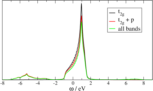
Figure 2: DOS of the vanadium t_2g-like Wannier functions of SrVO₃ produced by dmftproj, for 3 different choices of projection window. Black line: only vanadium t_2g bands, $\mathcal{W}=[-2.0,2.0]$ eV. Red line: vanadium t_2g and oxygen $p$ bands, $\mathcal{W}=[-8.0,2.0]$ eV. Green line: even larger window, $\mathcal{W}=[-8.0,8.0]$ eV. Note in the latter case the small additional weight around 7 eV.

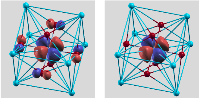
Figure 3: Real-space representation of the vanadium t_2g Wannier function of SrVO₃. Left plot: projection only to t_2g bands. Right plot: projection to all vanadium $d$ and oxygen $p$ bands. The blue and red colours indicate the negative and positive phases, respectively, of the Wannier function. Note the much better localisation of the $d$-like Wannier functions in the latter case, without weight around the oxygen positions. The Wannier functions are constructed using the dmftproj program, their real-space representations are generated with the help of the wplot program from the wien2wannier [10] package. Plots are produced using XCrysDen [26].

In practice it is much more convenient to work with projection operators, which transform quantities from the Bloch band basis to the Wannier orbital basis. We define these operators as

$$\hat{P}^{\alpha,\sigma}(\mathbf{k})=\sum_{m\in\mathcal{C}}|w_{\mathbf{k}m}^{\alpha,\sigma}\rangle\langle w_{\mathbf{k}m}^{\alpha,\sigma}|.$$ (3)

The matrix elements of these operators are calculated straight-forwardly using the above Wannier functions:

$$P_{m\nu}^{\alpha,\sigma}(\mathbf{k}) =\underset{\alpha^{\prime}m^{\prime}}{\sum}S_{m,m^{\prime}}^{\alpha,\alpha^{\prime}}\widetilde{P}_{m^{\prime}\nu}^{\alpha^{\prime},\sigma}(\mathbf{k})$$ (4)

$$\widetilde{P}_{m\nu}^{\alpha,\sigma}(\mathbf{k}) =\langle\tilde{\chi}_{m}^{\alpha,\sigma}|\psi_{\mathbf{k}\nu}^{\sigma}\rangle,\qquad\nu\in\mathcal{W}$$ (5)

These projectors can now be used to calculate, e.g., the local projected non-interacting Matsubara Green’s function from the DFT Green’s function,

$$G_{mn}^{0,\alpha}(i\omega_{n})=\sum_{\mathbf{k}}\sum_{\nu}P_{m\nu}^{\alpha}(\mathbf{k})\frac{1}{i\omega_{n}-\varepsilon_{\mathbf{k}\nu}+\mu}P_{n\nu}^{\alpha*}(\mathbf{k}),$$ (6)

where we have dropped the spin index for better readability. Note that throughout the paper we assume a proper normalisation of the momentum sum over $\mathbf{k}$ in the first Brillouin zone, i.e. $\sum_{\mathbf{k}}1=1$. From this non-interacting Green’s function one can calculate the density of states. As an example, we show in Fig. 2 the DOS for the prototypical material SrVO₃. Three different Wannier constructions are displayed. First, a projection where only the vanadium t_2g bands are taken into account is shown in black. The projection that comprises vanadium t_2g as well as the oxygen $p$ bands is shown in red, and the green line is the DOS for a projection using DFT bands up to 8 eV. The difference in the latter two projections is minor, and consists primarily in the small transfer of weight to large energies around 7 eV.

In Fig. 3 we show the real-space representation of the Wannier charge density. The left plot shows a t_2g-like Wannier function for a projection of t_2g bands only, which corresponds to the black line in Fig. 2. The right plot is the corresponding Wannier function when all bands are included in the projection. The effect of increasing the projection window is obvious: it results in a better localisation of the resulting Wannier functions.

All necessary steps to construct the orthonormalised set of projection operators from Wien2k DFT calculations is contained in the program dmftproj that is shipped with TRIQS/DFTTools. In Wien2k the Bloch functions are expanded in the LAPW basis set as

$$\begin{split}\psi_{\mathbf{k}\nu}^{\sigma}(\mathbf{r})&=\overset{N_{PW}}{\underset{\mathbf{G}}{\sum}}c_{\mathbf{G}}^{\nu,\sigma}(\mathbf{k})\underset{lm}{\sum}A_{lm}^{\alpha,\mathbf{k}+\mathbf{G}}u_{l}^{\alpha,\sigma}(r,E_{1l}^{\alpha})Y_{m}^{l}(\hat{r})\\ &+\overset{N_{lo}}{\underset{n_{lo}=1}{\sum}}c_{lo}^{\nu,\sigma}\left[A_{lm}^{\alpha,lo}u_{l}^{\alpha,\sigma}(r,E_{1l}^{\alpha})+B_{lm}^{\alpha,lo}\dot{u}_{l}^{\alpha,\sigma}(r,E_{1l}^{\alpha})\right]Y_{m}^{l}(\hat{r})+\\ &+\overset{N_{LO}}{\underset{n_{LO}=1}{\sum}}c_{LO}^{\nu,\sigma}\left[A_{lm}^{\alpha,LO}u_{l}^{\alpha,\sigma}(r,E_{1l}^{\alpha})+C_{lm}^{\alpha,LO}u_{l}^{\alpha,\sigma}(r,E_{2l}^{\alpha})\right]Y_{m}^{l}(\hat{r}),\end{split}$$ (7)

where $N_{PW}$ is the total number of plane waves in the basis set, $N_{lo}$ is the number of local orbitals, and $N_{LO}$ the corresponding number of auxiliary orbitals for semi-core states. For more details on the Wien2k basis set we refer the reader to the literature [22, 27, 24].

As initial localised orbitals $|\chi_{m}^{\alpha,\sigma}\rangle$ in our projective Wannier function construction, we choose the solutions of the Schrödinger equation within the muffin-tin sphere $\left|u_{l}^{\alpha,\sigma}(E_{1l})Y_{m}^{l}\right\rangle$ at the corresponding linearisation energy $E_{1l}$. Inserting this ansatz into Eq. 1 and using the orthogonality relations of the solutions of the Schrödinger equation allows to calculate the matrix elements of the projection operators. After some algebra one arrives at the expressions

$$\begin{split}\widetilde{P}_{m\nu}^{\alpha,\sigma}(\mathbf{k})&=\left\langle u_{l}^{\alpha,\sigma}(E_{1l})Y_{m}^{l}\right.\left|\psi_{\mathbf{k}\nu}^{\sigma}\right\rangle\\ &=A_{lm}^{\nu,\alpha}(\mathbf{k},\sigma)+\overset{}{\underset{n_{LO}=1}{\sum}}C_{lm,LO}^{\nu,\alpha}(\mathbf{k},\sigma),\end{split}$$ (8)

with contributions from the LAPW and/or APW+$lo$ orbitals

$$\begin{array}[]{ll}A_{lm}^{\nu,\alpha}(\mathbf{k},\sigma)&=\overset{N_{PW}}{\underset{\mathbf{G}}{\sum}}c_{\mathbf{G}}^{\nu,\sigma}(\mathbf{k})A_{lm}^{\alpha,\mathbf{k}+\mathbf{G}}\\ &+\overset{N_{lo}}{\underset{n_{lo}=1}{\sum}}c_{lo}^{\nu,\sigma}A_{lm}^{\alpha,lo}+\overset{N_{LO}}{\underset{n_{LO}=1}{\sum}}c_{LO}^{\nu,\sigma}A_{lm}^{\alpha,LO}\end{array}$$ (9)

as well as the contribution from the semi-core orbitals,

$$C_{lm,LO}^{\nu,\alpha}(\mathbf{k},\sigma)=c_{LO}^{\nu,\sigma}C_{lm}^{\alpha,LO}\left\langle u_{l}^{\alpha,\sigma}(E_{1l})Y_{m}^{l}|u_{l^{\prime}}^{\alpha,\sigma}(E_{l,LO})Y_{m^{\prime}}^{l^{\prime}}\right\rangle.$$ (10)

dmftproj takes all the necessary data from Wien2k, evaluates Eqs. 8 and 10 to obtain the matrix elements of the projection operators, Eqs. 4 and 5. Further information needed for the DMFT calculation are i) the rotation matrix from local to global coordinate systems, ii) the Kohn-Sham Hamiltonian within the projection window, and iii) the symmetry operation matrices for the BZ integration. All this information is extracted by dmftproj from the Wien2k output.

3.2 Usage

As a prerequisite a self-consistent Wien2k DFT calculation has to be performed. At this point, the further steps for the interface are

• writing of necessary data from the Wien2k calculation into files, which is done using the Wien2k command x lapw2 -almd,

• running dmftproj to calculate the projective Wannier functions,

• conversion of the text output files into the hdf5 file format using the Python modules provided.

After these steps, all necessary information for a DMFT calculation is stored in a single hdf5 file. For the details of these steps, and all input/output parameters we refer the reader to the extensive online documentation of TRIQS/DFTTools and the example below.

3.3 General interface for non-Wien2k users

The TRIQS/DFTTools package also contains an interface layer that can be used in many situations, albeit without the possibility of full charge self-consistency. In fact, as an input it takes the correlated subspace Hamiltonian $H_{mn}(\mathbf{k})$, where $m$ and $n$ are orbital indices, and the $\mathbf{k}$-mesh spans the first BZ. Unlike the Wien2k converter, the calculation is done exclusively in Wannier orbital space. The converter takes this $H_{mn}(\mathbf{k})$, together with information such as the quantum numbers of the correlated orbitals and the required electron density, and produces a hdf5 file that can be used for the DMFT calculations. We note that this interface is completely independent of how the $H_{mn}(\mathbf{k})$ is produced. It can use, for instance, output from Wannier90 [28, 29], which is available for many DFT codes, from NMTO calculations [30], or from any other tight-binding model representing the non-interacting electronic structure of the system.

4 One-shot DFT+DMFT calculations

⬇

1# imports and initialisations

2from pytriqs.applications.dft.sumk_dft import SumkDFT

3

4SK = SumkDFT(hdf_file = ’YourDFTDMFTcalculation.h5’)

5S = Solver(...) # appropriate constructor parameters to be defined

6n_loops = 15 # define the number of DMFT loops

7

8for iteration_number in range(n_loops) : # start the DMFT loop

9

10 # set the self-energy as an attribute of the class:

11 SK.set_Sigma(Sigma_imp = [ S.Sigma_iw ])

12 # calculate the chemical potential:

13 chemical_potential = SK.calc_mu()

14 # extract the local Green’s function:

15 S.G_iw << SK.extract_G_loc()[0]

16 # finally get G0 (input for the Solver):

17 S.G0_iw << inverse(S.Sigma_iw + inverse(S.G_iw))

18

19 # now solve the impurity problem:

20 S.solve(...) # appropriate solve parameters to be defined

21

22 # calculate the new double counting correction:

23 dm = S.G_iw.density()

24 SK.calc_dc(dm, U_interact=U, J_hund=J, orb=0, use_dc_formula=0)

25

26# save the final results into an archive

27from pytriqs.archive import HDFArchive

28import pytriqs.utility.mpi as mpi

29if mpi.is_master_node():

30 with HDFArchive(’YourDFTDMFTcalculation.h5’,’a’) as ar:

31 ar[’G’] = S.G_iw

32 ar[’Sigma’] = S.Sigma_iw

Listing 1: Sketch of the Python script for the DMFT self-consistency loop in one-shot DFT+DMFT calculations. Note that the solver imports, construction and execution must be appropriately added and modified.

As mentioned in the introduction, TRIQS/DFTTools provides simple modules that allow the compact and efficient implementation of the DMFT self-consistency cycle. We will illustrate how to use the package by giving a one-to-one correspondence of the code statements to the necessary equations. In this section we give a simple Python script for so-called ‘one-shot’ DFT+DMFT calculations without full charge self-consistency. Note that the construction of the Wannier functions and the conversion procedures discussed in the previous section have already been performed. We assume that the hdf5 archive for the calculation, where everything is stored, is called YourDFTDMFTcalculation.h5. Furthermore, we assume that a suitable method to solve the quantum impurity problem is available, such as the TRIQS/CTHYB solver [18]. Note that TRIQS/DFTTools itself does not provide any impurity solver.

The DMFT calculation as given in Lst. 1 consists of the following steps. First, we initialise our calculation as done in lines 2 to 6 of Lst. 1. The SumkDFT module is loaded and initialised with the previously generated hdf5 archive YourDFTDMFTcalculation.h5. We initialise a solver module, which is used for the solution of the Anderson impurity model, for instance, the TRIQS/CTHYB package [18]. It is important that the user is familiar with the details of this solver initialisation, including set-up of the interaction matrix, definition of the interaction parameters $U$ and $J$, etc. We request $n_{\rm loops}=15$ self-consistency cycles to be done. This number has of course to be adapted to the problem at hand in order to reach convergence. After this initialisation step, we begin the self-consistency loop:

1. Impurity self-energy (line 11): The command SK.set_Sigma(Sigma_imp = [ S.Sigma_iw ]) takes an impurity self-energy $\Sigma_{mm^{\prime}}^{\rm{imp}}(i\omega)$ in orbital space, and sets it as a member of the SK class. We assume that the object S.Sigma_iw is defined in the solver. At initialisation, the self-energy can be set to zero, or to its Hartree value to speed up convergence.

2. Chemical potential determination (line 13): The chemical potential is set according to the definition

   $$N_{e}=\mathrm{Tr}\sum_{\mathbf{k}}\Big{[}(i\omega_{n}-\varepsilon_{\mathbf{k}\nu}+\mu)\delta_{\nu\nu^{\prime}}-\Sigma_{\nu\nu^{\prime}}\Big{]}^{-1}e^{i\omega_{n}0^{+}},$$ (11)

   where $N_{e}$ is the required electronic density in the projection window. Please note that the operation $[\cdots]^{-1}$ denotes matrix inversions throughout this paper. The self-energy in band space is defined by

   $$\Sigma_{\nu\nu^{\prime}}(\mathbf{k},i\omega_{n})=\sum_{\alpha,mm^{\prime}}P_{m\nu}^{\alpha*}(\mathbf{k})\left(\Sigma_{mm^{\prime}}^{\rm{imp}}(i\omega_{n})-\Sigma^{\rm{DC}}\right)P_{m^{\prime}\nu^{\prime}}^{\alpha}(\mathbf{k}).$$ (12)

   We use the projectors as introduced in Sec. 3, as well as a double-counting correction $\Sigma^{\rm{DC}}$ [2].

3. Local Green’s function (line 15): The local Green’s function is calculated as

   $$G_{mm^{\prime}}^{\mathrm{loc,\alpha}}(i\omega_{n})=\sum_{\mathbf{k}}\sum_{\nu\nu^{\prime}}P_{m\nu}^{\alpha}(\mathbf{k})\Big{[}(i\omega_{n}-\varepsilon_{\mathbf{k}\nu}+\mu)\delta_{\nu\nu^{\prime}}-\Sigma_{\nu\nu^{\prime}}(\mathbf{k},i\omega_{n})\Big{]}^{-1}P_{m^{\prime}\nu^{\prime}}^{\alpha*}(\mathbf{k}),$$ (13)

   where $\alpha$ is the index of the correlated atom in the unit cell. In Lst. 1 we have only one inequivalent correlated atomic shell, so we need to take only $\alpha=0$.

4. New hybridisation function (line 17): We now calculate the new Weiss field for the impurity problem using the Dyson equation

   $$\mathcal{G}_{mm^{\prime}}^{0}(i\omega_{n})=\left[\Sigma_{mm^{\prime}}^{\rm imp}(i\omega_{n})+\left[G_{mm^{\prime}}^{\mathrm{loc}}(i\omega_{n})\right]^{-1}\right]^{-1}.$$ (14)

5. Solve the impurity problem (line 20): We call the solver method S.solve with the relevant parameters. Again, the user must be familiar with the usage of the solver of choice and its parameters, in order to produce meaningful and physically sound results. The solver produces the Green’s function and the self-energy of the interacting impurity problem. Following the TRIQS/CTHYB convention, we assume for the example given here that the Green’s function and the self-energy are stored in S.G_iw and S.Sigma_iw, respectively.

6. Double counting (lines 23-24): We calculate a new double counting (DC) correction from the impurity density matrix (line 23). As additional parameters one needs to provide a Hubbard interaction value $U$ and Hund’s exchange $J$, which have to be in accordance with the definition of the interaction matrix. TRIQS/DFTTools offers three different DC corrections: The flag use_dc_formula=0 corresponds to the fully-localised limit (FLL) correction, use_dc_formula=1 is a variant of FLL that is used for Kanamori-type Hamiltonians [31], and use_dc_formula=2 is the around-mean-field (AMF) correction. This step completes the self-consistency loop.

Steps 1 to 6 are now iterated until convergence. After that, we can save the final solution into the hdf5 archive, as done in lines 27 to 32. We want to note here that it is sometimes useful to save all data produced by the user in a separate subgroup, e.g. dmft_results, in order to have a clean structure in the hdf5 archive. For details how to handle the hdf5 archive we refer the reader to Ref. [21] and the online TRIQS documentation.

We want to stress here that this simple script of about 30 lines of Python code is sufficient for a full DFT+DMFT calculation, which is possible only thanks to the modular structure of TRIQS/DFTTools and TRIQS.

5 Full charge self-consistency

Figure 4: (Colour online) Sketch of the self-consistency cycle of fully charge self-consistent calculations.

The one-shot DFT+DMFT calculation can be extended to a fully charge self-consistent calculation with only marginal additional effort. The basic concept is general, but the implementation will depend of course on the DFT code that you wish to use for the calculations. We are presenting the interface to the Wien2k DFT package, which is the first interface implemented in TRIQS/DFTTools. We describe this interface below. Work is in progress to include more DFT packages, in particular VASP [32, 33].

First of all, we want to stress that the fully charge self-consistent calculation is controlled by Wien2k scripts. That is why a sound knowledge of Wien2k and how it is used is absolutely necessary for the considerations in this section.

⬇

1SK.set_Sigma(Sigma_imp = [ S.Sigma_iw ])

2chemical_potential = SK.calc_mu( precision = 0.000001 )

3dN, d = SK.calc_density_correction(filename = ’case.qdmft’)

4SK.save([’chemical_potential’,’dc_imp’,’dc_energ’])

Listing 2: Code snippet for the calculation of the corrected charge density due to correlations

As shown in Fig. 4, the idea is to extend the existing Wien2k self-consistency loop by including a DMFT step. Instead of simply calculating the charge density from the Kohn-Sham orbitals as in standard DFT (lapw2 step in Wien2k), we supplement this charge density with correlation effects. Therefore, the Python scripts that control the DMFT iteration have to be modified:

• We do not start each DMFT iteration from scratch, but instead from the previous iteration. This is most conveniently done by storing all necessary data in the hdf5 archive.

• One DMFT iteration ($n_{\rm loops}=1$) per full self-consistency cycle is usually sufficient. In cases where convergence is problematic, more iterations may be needed.

• In order to calculate the correction to the charge density, one has to calculate the density matrix from the correlated Green’s function at the end of the DMFT step, as shown in Lst. 2. The first two lines set the chemical potential more accurately. The important step is line 3, where the correlated density matrix is calculated in Bloch band space

  $$N^{k}_{\nu\nu^{\prime}} =\sum_{n}G_{\nu\nu^{\prime}}(\mathbf{k},i\omega_{n})e^{i\omega_{n}0^{+}}$$ (15)

  $$G_{\nu\nu^{\prime}}(\mathbf{k},i\omega_{n}) =\Big{[}(i\omega_{n}-\varepsilon_{\mathbf{k}\nu}+\mu)\delta_{\nu\nu^{\prime}}-\Sigma_{\nu\nu^{\prime}}(\mathbf{k},i\omega_{n})\Big{]}^{-1},$$ (16)

  where $\Sigma_{\nu\nu^{\prime}}(\mathbf{k},i\omega_{n})$ is given by Eq. 12. This non-diagonal density matrix is used instead of the Kohn-Sham density matrix to calculate the charge density in x lapw2 -qdmft, see Fig. 4. Line 4 in Lst. 2 saves properties to the hdf5 archive such that they are available in the next iteration.

Compared to one-shot calculations, the fully charge self-consistent calculations are in general not much more demanding. As a rough guide, the additional computational effort due to an increased number of self-consistency loops is normally around 50%. Of course, this extra effort depends largely on the problem at hand and whether the DMFT corrections to the charge density are relevant or not.

This charge self-consistent implementation also allows the calculation of total energies from DFT+DMFT. The detailed formulas and their derivation can be found in Ref. [34] and references therein.

For more options of the TRIQS/DFTTools modules, as well as a complete example script and tutorial for a charge self-consistent calculation, including total energy calculation, we refer the reader to the online documentation of TRIQS/DFTTools.

6 Post-processing

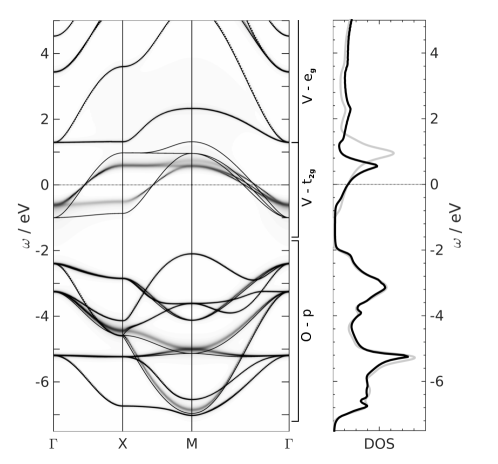
Figure 5: Left: Correlated band structure of SrVO₃ (grey-shaded plot) compared to the DFT band structure (black lines). Right: Correlated local spectral function (black line) and DFT DOS (grey line).

The main output of a DMFT calculation, be it one-shot or fully charge self-consistent, is the interacting Green’s function and the self-energy. However, in many cases one is interested in other quantities that are more closely connected to observables of experiments. For that reason TRIQS/DFTTools provides methods to further process the data and calculate some physical properties

• (orbitally-projected) density of states

• correlated band structures (spectral function $A(k,\omega)$)

• transport properties (resistivity, thermopower, optical conductivity)

For all these methods one needs to use a real-frequency self-energy. In case the solver provides only quantities on the Matsubara axis, one has to analytically continue the data, by methods like Pade approximants [21], the maximum entropy method [35], or others.

DOS and band structure. These two quantities are very similar in terms of equations, since they are both imaginary parts of retarded Green’s functions. For the band structure, we use

$$A(\mathbf{k},\omega)=-\frac{1}{\pi}\mathrm{Tr}\,\mathrm{Im}\,G_{\nu\nu^{\prime}}(\mathbf{k},\omega+i0^{+}),$$ (17)

where the Green’s function is defined equivalently to Eq. 16, but using a real-frequency self-energy. The trace is taken in matrix space of Bloch indices $\nu,\nu^{\prime}$. Summing this quantity over the first BZ gives the local spectral function.

As an example, we show in Fig. 5 a comparison of the DFT and the DFT+DMFT band structures (left) as well as the local spectral function and DOS (right) of SrVO₃. The projective Wannier functions were calculated in a large energy window of $[-8.5,7.5]$ eV. The impurity problem was solved using the TRIQS/CTHYB solver with interaction parameters $U=6.0$ eV and $J=0.65$ eV, and an analytic continuation was performed using stochastic maximum entropy [36].

The thin black lines are the DFT results. One can clearly identify the mass renormalisation of the t_2g bands, which is a bit smaller than 2 in our calculation. The oxygen $p$, as well as the vanadium e_g states are only marginally affected. However, due to the hybridisation between vanadium t_2g and oxygen $p$ states, the bands between $-7$ and $-2$ eV acquire a finite width.

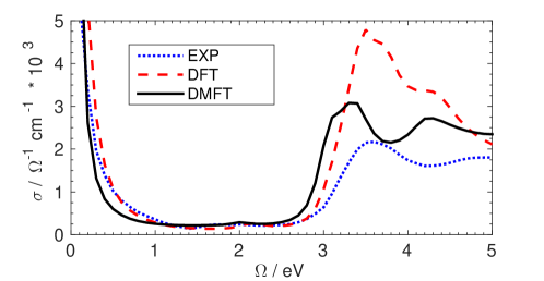
Figure 6: Optical conductivity of SrVO₃ calculated from the DFT+DMFT result (black solid line) and directly from DFT (red dashed line) compared to experimental data from Ref. [37] (blue dotted line).

Transport properties. These are evaluated in the Kubo linear-response formalism [5] neglecting vertex corrections [38, 39], and at the moment their computation is based on the Wien2k DFT code. In addition to the self-energy, one also needs the velocities $v^{\alpha}(\mathbf{k})$ which are proportional to the matrix elements of the momentum operator in direction $\alpha=\{x,y,z\}$, calculated with the Wien2k optics package [40]. The conductivity and the Seebeck coefficient for the combination of directions $\alpha\alpha^{\prime}$ are defined as

$$\sigma^{\alpha\alpha^{\prime}}=\beta e^{2}K_{0}^{\alpha\alpha^{\prime}}\ \ \ \text{and}\ \ \ S^{\alpha\alpha^{\prime}}=-\frac{k_{B}}{|e|}\frac{K_{1}^{\alpha\alpha^{\prime}}}{K_{0}^{\alpha\alpha^{\prime}}}$$ (18)

with $\beta$ the inverse temperature. The kinetic coefficients $K_{n}^{\alpha\alpha^{\prime}}$ are given by

$$K_{n}^{\alpha\alpha^{\prime}}=N_{sp}\pi\hbar\int{d\omega\left(\beta\omega\right)^{n}f\left(\omega\right)f\left(-\omega\right)\Gamma^{\alpha\alpha^{\prime}}\left(\omega,\omega\right)}.$$ (19)

Here $N_{sp}$ is the spin factor and $f(\omega)$ is the Fermi function. The transport distribution $\Gamma^{\alpha\alpha^{\prime}}\left(\omega_{1},\omega_{2}\right)$ is defined as

$$\Gamma^{\alpha\alpha^{\prime}}\left(\omega_{1},\omega_{2}\right)=\frac{1}{V}\sum_{k}\mathrm{Tr}\,\left(v^{\alpha}(\mathbf{k})A(\mathbf{k},\omega_{1})v^{\alpha^{\prime}}(\mathbf{k})A(\mathbf{k},\omega_{2})\right),$$ (20)

where $V$ is the unit cell volume. In multi-band systems the velocities $v^{\alpha}(\mathbf{k})$ and the spectral function $A(\mathbf{k},\omega)$ are Hermitian matrices in the band indices $\nu$ and $\nu^{\prime}$. The frequency-dependent optical conductivity is given by

$$\sigma^{\alpha\alpha^{\prime}}(\Omega)=N_{sp}\pi e^{2}\hbar\int{d\omega\Gamma^{\alpha\alpha^{\prime}}(\omega+\Omega,\omega)\frac{f(\omega)-f(\omega+\Omega)}{\Omega}}.$$ (21)

A related implementation, also using full dipole matrix elements but in the framework of maximally localised Wannier functions, has recently been published as the woptic package [41].

We illustrate the calculation of transport properties again for the example of SrVO₃. We apply the same setup as for the calculation of the band structure given above. For the $\mathbf{k}$-summation, we use 4495 $\mathbf{k}$-points in the irreducible BZ. At $T=290$ K we obtain a DC resistivity of $47$ $\mu\Omega$cm, which compares reasonably well with the experimental value of $70$ $\mu\Omega$cm [42]. The Seebeck coefficient, $-8$ $\mu$V/K in our calculation, agrees remarkably well with the experimental room temperature value of about $-11$ $\mu$V/K [43]. The same holds for the optical conductivity (Fig. 6) obtained from DFT+DMFT (black solid line) when compared to experimental results (blue dotted line). To show the effect of the correlations, we also present results without self-energy (red dashed line), which corresponds to evaluating the optical conductivity directly from DFT. Sometimes, scattering processes not included in plain DFT+DMFT calculations (e.g., phonons, impurities, or non-local fluctuations) are important. In this case, the calculated resistivity constitutes a lower bound to the expected experimental value. Note that for all transport calculations the convergence with the number of $\mathbf{k}$-points is essential and has to be checked carefully.

Further details on the use of these tools, including all options and parameters, are given in the online documentation.

7 Getting started

Detailed information on the installation procedure can be found on the TRIQS/DFTTools website and current issues and updates are available on GitHub.

7.1 Obtaining TRIQS/DFTTools

The TRIQS/DFTTools source code is available publicly and can be obtained by cloning the repository on the GitHub website at https://github.com/TRIQS/dft_tools. As the TRIQS project, including its applications, is continuously improving, we strongly recommend users to obtain TRIQS and its applications, including TRIQS/DFTTools, from GitHub. Bugfixes to possible issues are also applied to the GitHub source.

For users that wish to have a more stable version of the code, without the latest bugfixes and functionalities, we suggest downloading the latest tagged version from the GitHub releases page https://github.com/TRIQS/dft_tools/releases.

7.2 Installation

Once the TRIQS library has been installed properly, the installation of TRIQS/DFTTools is straightforward. As for TRIQS we use the cmake tool to configure, build and test the application. With the TRIQS library installed in /path/to/TRIQS/install/dir, the TRIQS/DFTTools application can be installed by

$ git clone https://github.com/TRIQS/dft_tools.git src
$ mkdir build_dft_tools && cd build_dft_tools
$ cmake -DTRIQS_PATH=/path/to/TRIQS/install/dir ../src
$ make
$ make test
$ make install

This will first download the code to the src directory, then build, test, and install the application in the same location as the TRIQS library.

7.3 Citation policy

We kindly request that the present paper is cited in any published work using the TRIQS/DFTTools package. Furthermore, we request that the original works to this package, Refs. [24] for the first implementation and [34] for full charge self-consistency, are cited accordingly, too. In addition, since this package is based on the TRIQS library, a citation to [21] is also requested, along with the appropriate citation to any solver used, e.g. TRIQS/CTHYB [18].

7.4 Contributing

TRIQS/DFTTools, as an application of TRIQS, is an open source project. We appreciate feedback and contributions from the user community to this package. Issues and bugs can be reported on the GitHub website (https://github.com/TRIQS/dft_tools/issues). Before starting major contributions, please coordinate with the team of TRIQS/DFTTools developers.

8 Summary

In summary we presented the TRIQS/DFTTools package, an application based on the TRIQS library. This package provides the necessary tools for setting up DFT+DMFT calculations. We have shown simple examples demonstrating how the code can be used to calculate Wannier functions, spectral functions, as well as transport properties of the prototypical material SrVO₃.

9 Acknowledgements

We gratefully acknowledge discussions, comments, and feedback from the user community, and ongoing collaborations with A. Georges and S. Biermann. M. Aichhorn, M. Zingl, and G. J. Kraberger acknowledge financial support from the Austrian Science Fund (Y746, P26220, F04103), and great hospitality at Collège de France, École Polytechnique, and CEA Saclay. L. Pourovskii acknowledges the financial support of the Ministry of Education and Science of the Russian Federation in the framework of Increase Competitiveness Program of NUST MISiS (No. K3-2015-038). L. Pourovskii and V. Vildosola acknowledge financial support from ECOS-A13E04. O. E. Peil acknowledges support from the Swiss National Science Foundation (program NCCR-MARVEL). P. Seth acknowledges support from ERC Grant No. 617196-CorrelMat. O. Parcollet and P. Seth acknowledge support from ERC Grant No. 278472-MottMetals. J. Mravlje acknowledges discussions with J. Tomczak and support of Slovenian Research Agency (ARRS) under Program P1-0044.

References

- [1] M. Imada, A. Fujimori, Y. Tokura, Metal-insulator transitions, Rev. Mod. Phys. 70 (1998) 1039–1263.
- [2] V. I. Anisimov, F. Aryasetiawan, A. I. Lichtenstein, First-principles calculations of the electronic structure and spectra of strongly correlated systems: the LDA + U method, J. Phys.: Condens. Matt. 9 (4) (1997) 767.
- [3] A. Georges, G. Kotliar, W. Krauth, M. J. Rozenberg, Dynamical mean-field theory of strongly correlated fermion systems and the limit of infinite dimensions, Rev. Mod. Phys. 68 (1996) 13–125.
- [4] V. I. Anisimov, A. I. Poteryaev, M. A. Korotin, A. O. Anokhin, G. Kotliar, First-principles calculations of the electronic structure and spectra of strongly correlated systems: dynamical mean-field theory, J. Phys.: Condensed Mat. 9 (35) (1997) 7359.
- [5] G. Kotliar, S. Y. Savrasov, K. Haule, V. S. Oudovenko, O. Parcollet, C. A. Marianetti, Electronic structure calculations with dynamical mean-field theory, Rev. Mod. Phys. 78 (2006) 865–951.
- [6] L. V. Pourovskii, B. Amadon, S. Biermann, A. Georges, Self-consistency over the charge density in dynamical mean-field theory: A linear muffin-tin implementation and some physical implications, Phys. Rev. B 76 (23) (2007) 235101.
- [7] V. I. Anisimov, D. E. Kondakov, A. V. Kozhevnikov, I. A. Nekrasov, Z. V. Pchelkina, J. W. Allen, S.-K. Mo, H.-D. Kim, P. Metcalf, S. Suga, A. Sekiyama, G. Keller, I. Leonov, X. Ren, D. Vollhardt, Full orbital calculation scheme for materials with strongly correlated electrons, Phys. Rev. B 71 (2005) 125119.
- [8] F. Lechermann, A. Georges, A. Poteryaev, S. Biermann, M. Posternak, A. Yamasaki, O. K. Andersen, Implementation of dynamical mean-field theory using Wannier functions: a flexible route to electronic structure calculations of strongly correlated materials, Phys. Rev. B 74 (2006) 125120.
- [9] K. Haule, C.-H. Yee, K. Kim, Dynamical mean-field theory within the full-potential methods: Electronic structure of CeIrIn5, CeCoIn5, and CeRhIn5, Phys. Rev. B 81 (19) (2010) 195107.
- [10] J. Kuneš, R. Arita, P. Wissgott, A. Toschi, H. Ikeda, K. Held, Wien2wannier: From linearized augmented plane waves to maximally localized wannier functions, Comput. Phys. Commun. 181 (11) (2010) 1888 – 1895.
- [11] B. Amadon, A self-consistent DFT+DMFT scheme in the projector augmented wave method: applications to cerium, Ce2O3 and Pu2O3 with the HubbardI solver and comparison to DFT+U, J. Phys.: Condens. Matt. 24 (7) (2012) 075604.
- [12] H. Park, A. J. Millis, C. A. Marianetti, Computing total energies in complex materials using charge self-consistent DFT + DMFT, Phys. Rev. B 90 (2014) 235103.
- [13] A. N. Rubtsov, V. V. Savkin, A. I. Lichtenstein, Continuous-time quantum Monte Carlo method for fermions, Phys. Rev. B 72 (3) (2005) 035122.
- [14] P. Werner, A. Comanac, L. de’ Medici, M. Troyer, A. J. Millis, Continuous-time solver for quantum impurity models, Phys. Rev. Lett. 97 (2006) 076405.
- [15] P. Werner, A. J. Millis, Hybridization expansion impurity solver: General formulation and application to kondo lattice and two-orbital models, Phys. Rev. B 74 (2006) 155107.
- [16] K. Haule, Quantum monte carlo impurity solver for cluster dynamical mean-field theory and electronic structure calculations with adjustable cluster base, Phys. Rev. B 75 (2007) 155113.
- [17] E. Gull, A. J. Millis, A. I. Lichtenstein, A. N. Rubtsov, M. Troyer, P. Werner, Continuous-time monte carlo methods for quantum impurity models, Rev. Mod. Phys. 83 (2011) 349–404.
- [18] P. Seth, I. Krivenko, M. Ferrero, O. Parcollet, TRIQS/CTHYB: A continuous-time quantum monte carlo hybridization expansion solver for quantum impurity problems, arxiv.org/abs/1507.00175, accepted for publication in Comput. Phys. Commun.
- [19] J. Mravlje, M. Aichhorn, T. Miyake, K. Haule, G. Kotliar, A. Georges, Coherence-incoherence crossover and mass renormalization puzzles in Sr2RuO4, Phys. Rev. Lett. 106 (2011) 096401.
- [20] Z. V. Pchelkina, I. A. Nekrasov, T. Pruschke, A. Sekiyama, S. Suga, V. I. Anisimov, D. Vollhardt, Evidence for strong electronic correlations in the spectra of , Phys. Rev. B 75 (2007) 035122.
- [21] O. Parcollet, M. Ferrero, T. Ayral, H. Hafermann, I. Krivenko, L. Messio, P. Seth, TRIQS: A toolbox for research on interacting quantum systems, Comput. Phys. Commun. 196 (2015) 398 – 415.
- [22] P. Blaha, K. Schwarz, G. Madsen, D. Kvasnicka, J. Luitz, WIEN2k, An augmented Plane Wave + Local Orbitals Program for Calculating Crystal Properties, Techn. Universitat Wien, Austria, ISBN 3-9501031-1-2., 2001.
- [23] C. Martins, M. Aichhorn, L. Vaugier, S. Biermann, Reduced effective spin-orbital degeneracy and spin-orbital ordering in paramagnetic transition-metal oxides: versus , Phys. Rev. Lett. 107 (2011) 266404.
- [24] M. Aichhorn, L. Pourovskii, V. Vildosola, M. Ferrero, O. Parcollet, T. Miyake, A. Georges, S. Biermann, Dynamical mean-field theory within an augmented plane-wave framework: Assessing electronic correlations in the iron pnictide LaFeAsO, Phys. Rev. B 80 (2009) 085101.
- [25] D. Korotin, A. Kozhevnikov, S. Skornyakov, I. Leonov, N. Binggeli, V. Anisimov, G. Trimarchi, Construction and solution of a Wannier-functions based Hamiltonian in the pseudopotential plane-wave framework for strongly correlated materials, Eur. Phys. J. B 65 (1) (2008) 91–98.
- [26] A. Kokalj, Computer graphics and graphical user interfaces as tools in simulations of matter at the atomic scale, Comp. Mater. Sci. 28 (2003) 155.
- [27] D. J. Singh, Plane waves, pseudopotentials and the LAPW method, Kluwer, Dordrecht, 1994.
- [28] N. Marzari, D. Vanderbilt, Maximally localized generalized wannier functions for composite energy bands, Phys. Rev. B 56 (1997) 12847.
- [29] I. Souza, N. Marzari, D. Vanderbilt, Maximally localized wannier functions for entangled energy bands, Phys. Rev. B 65 (2001) 035109.
- [30] O. K. Andersen, T. Saha-Dasgupta, Muffin-tin orbitals of arbitrary order, Phys. Rev. B 62 (2000) R16219.
- [31] K. Held, Electronic structure calculations using dynamical mean field theory, Adv. Phys. 56 (6) (2007) 829–926.
- [32] G. Kresse, J. Furthmüller, Efficient iterative schemes for ab initio total-energy calculations using a plane-wave basis set, Phys. Rev. B 54 (1996) 11169–11186.
- [33] G. Kresse, D. Joubert, From ultrasoft pseudopotentials to the projector augmented-wave method, Phys. Rev. B 59 (1999) 1758–1775.
- [34] M. Aichhorn, L. Pourovskii, A. Georges, Importance of electronic correlations for structural and magnetic properties of the iron pnictide superconductor LaFeAsO, Phys. Rev. B 84 (2011) 054529.
- [35] M. Jarrell, J. E. Gubernatis, Bayesian inference and the analytic continuation of imaginary-time quantum Monte Carlo data, Phys. Rep. 269 (3) (1996) 133–195.
- [36] K. S. D. Beach, Identifying the maximum entropy method as a special limit of stochastic analytic continuation, arxiv/0403055.
- [37] H. Makino, I. H. Inoue, M. J. Rozenberg, I. Hase, Y. Aiura, S. Onari, Bandwidth control in a perovskite-type -correlated metal . II. Optical spectroscopy, Phys. Rev. B 58 (1998) 4384–4393.
- [38] A. Khurana, Electrical conductivity in the infinite-dimensional Hubbard model, Phys. Rev. Lett. 64 (1990) 1990–1990.
- [39] H. T. Dang, J. Mravlje, A. Georges, A. J. Millis, Band structure and terahertz optical conductivity of transition metal oxides: Theory and application to , Phys. Rev. Lett. 115 (2015) 107003.
- [40] C. Ambrosch-Draxl, J. O. Sofo, Linear optical properties of solids within the full-potential linearized augmented planewave method, Comput. Phys. Commun. 175 (1) (2006) 1 – 14.
- [41] E. Assmann, P. Wissgott, J. Kunes, A. Toschi, P. Blaha, K. Held, woptic: Optical conductivity with wannier functions and adaptive k-mesh refinement, Computer Physics Communications in press (2015) –.
- [42] I. H. Inoue, O. Goto, H. Makino, N. E. Hussey, M. Ishikawa, Bandwidth control in a perovskite-type -correlated metal I. Evolution of the electronic properties and effective mass, Phys. Rev. B 58 (1998) 4372–4383.
- [43] P. Dougier, J. C. Fan, J. B. Goodenough, Etude des proprietes magnetiques, electriques et optiques des phases de structure perovskite SrVO2.90 et SrVO3, J. Solid State Chem. 14 (3) (1975) 247 – 259.