Fully Distributed Adaptive Output Feedback Protocols for Linear Multi-Agent Systems with Directed Graphs: A Sequential Observer Design Approach

Abstract

This paper studies output feedback consensus protocol design problems for linear multi-agent systems with directed graphs. We consider both leaderless and leader-follower consensus with a leader whose control input is nonzero and bounded. We propose a novel sequential observer design approach, which makes it possible to design fully distributed adaptive output feedback protocols that the existing methods fail to accomplish. With the sequential observer architecture, we show that leaderless consensus can be achieved for any strongly connected directed graph in a fully distributed manner, whenever the agents are stabilizable and detectable. For the case with a leader of bounded control input, we further present novel distributed adaptive output feedback protocols, which include nonlinear functions to deal with the effect of the leaders’s nonzero control input and are able to achieve leader-follower consensus for any directed graph containing a directed spanning tree with the leader as the root.

I Introduction

Over the past decade, the consensus control problem of multi-agent systems has emerged as a focal research topic in the field of control, due to its various applications to, e.g., UAV formation flying, multi-point surveillance, and distributed reconfigurable sensor networks [1, 2]. Considerable work from different perspectives has been conducted on consensus and other related cooperative control problems; see the recent papers [3, 4, 5, 1, 6, 2], the monographs [7, 8], and the references therein.

Existing consensus algorithms can be essentially divided into two broad categories, namely, consensus without a leader (i.e., leaderless consensus) and consensus with a leader, whereas the latter ia also called leader-follower consensus or distributed tracking. In a leader-follower consensus problem, it is often the case that the leader may need to implement its own control actions to achieve certain objectives, e.g., to reach a desirable consensus trajectory or to avoid hazardous obstacles. Thus, compared to leaderless consensus, an additional difficulty with leader-follower consensus lies in how to deal with the effect of the leader’s control input which is available to at most a small subset of the followers.

I-A Motivations and Related Works

A central task in consensus studies is to design distributed consensus protocols based on only the local information of each agent and its neighbors to ensure that the states of the agents reach an agreement. In most of the previous works on consensus, e.g., [9, 10, 5, 11, 12, 13], which address the consensus problem of integrator-type, general linear and Lipschitz nonlinear multi-agent systems, the design of the consensus protocols requires the knowledge of certain connectivity of the communication graph. The connectivity for undirected graphs can be measured by the smallest nonzero eigenvalue of the corresponding Laplacian matrix [3], while for directed graphs the smallest positive real part of the eigenvalues of the Laplacian matrix [5] or other similar quantities are typically used [13]. Since the connectivity measures require computing the nonzero eigenvalues of the Laplacian matrix associated with the entire communication graph, the consensus protocols in these works require in essence global information of the graph which cannot be determined in a fully distributed manner.

Fully distributed consensus protocols, nevertheless, can be developed by implementing adaptive laws to dynamically update the coupling weights of neighboring agents, thus removing the aforementioned requirement on the global eigenvalue information. Such adaptive consensus protocols are proposed in [14, 15] for linear multi-agent systems, which depend on only local information of each agent and its neighbors. Similar adaptive schemes are presented in [16, 17] for second-order nonlinear agents. Note that the adaptive protocols in [14, 15, 16, 17] are applicable to only undirected communication graphs. Due to the asymmetry of the corresponding Laplacian matrices, however, the development of distributed adaptive consensus protocols poses a more difficult problem with directed graphs. By introducing monotonically increasing functions as a means to provide additional freedom for design, a distributed adaptive consensus protocol is constructed in [18], for directed graphs containing a directed spanning tree in which the leader is the root node. Another adaptive protocol is presented in [19], which can be modified using the $\sigma$-modification technique so that it is robust in the presence of bounded external disturbances. It is worth pointing out, however, that the protocols in [18, 19] rely on the relative states of neighboring agents, which may not be available in general. How to design fully distributed adaptive output feedback consensus protocols using only local output information appears much more challenging. Except those protocols proposed in [20] for quite special minimum-phase and relative-degree-one agents, designing fully distributed output feedback protocols for general linear multi-agent systems with directed graphs remains to be an open issue.

The aforementioned works are concerned with the leaderless consensus problem or distributed tracking problem for the case where the leader is of zero control input. The distributed tracking problem in the presence of a leader having a nonzero control input is generally more difficult and has been addressed in [21, 22, 23, 24, 14, 25]. In particular, the authors in [21] present nonsmooth controllers for first- and second-order integrators in the absence of velocity or acceleration measurements. The controllers in [21] incorporate discontinuous functions commonly found in the sliding mode control literature, which are meant to cope with the leader’s bounded control input. The authors in [22, 23, 24] address a distributed coordinated tracking and containment control problem, for multiple Euler-Lagrange systems with one or more dynamic leaders. Distributed static and adaptive protocols are given in [14, 25] for general linear multi-agent systems with a leader of bounded control input. It is worth noting that one common assumption in [21, 14, 25] is that the subgraph among the followers is undirected. The case where this subgraph is directed remains unsolved for general linear multi-agent systems. The main obstacle lies in the unpleasant interrelations between the nonlinear functions used to deal with the leader’s control input and the directed subgraph among followers.

I-B Our Contributions

In this paper, we address the distributed adaptive output feedback consensus protocol design problem for general linear multi-agent systems with directed communication graphs. In this setting, the relative states of neighboring agents are not available, but only local output information is accessible. Both the cases with and without a leader of bounded control input are studied. Note that simply combining the techniques for the state feedback case (e.g., those proposed in [18, 19]) and distributed adaptive observer-type protocols (e.g., in [14]) for undirected graphs will not yield distributed adaptive output feedback consensus protocols applicable to general directed graphs. The main reason is that the monotonically increasing functions introduced in [18, 19], when used for observer-type adaptive protocols in [14], will still depend on the relative states of neighboring agents. This motivates us to seek for novel methods to design distributed output feedback consensus protocols.

To circumvent the difficulties alluded to above, in this paper we propose a two-step, sequential observer design (SOD) method, which consists of designing first a local observer and next a distributed observer. Here the local observer is employed to estimate from an agent’s output the agent’ state, while the distributed observer operates on the local state estimates and generates the control input; neither of these observers uses the state information of the agents. Utilizing this novel SOD architecture, two types of distributed adaptive output feedback consensus protocols are developed for the leaderless consensus problem, which exchange the local estimates among neighboring agents via the communication graph and implement adaptive laws to update the time-varying coupling weights among the agents. As such, these two adaptive protocols uses only the local output information and achieve leaderless consensus in a fully distributed manner, for any strongly connected directed graph. This constitutes one of our main contributions in this paper.

Another main result of this paper concerns the leader-follower consensus with a leader of bounded control input. We propose a distributed discontinuous adaptive output feedback protocol, to solve the consensus problem, which includes discontinuous nonlinear functions to deal with the effect of the leaders’s nonzero control input. It is shown that the discontinuous adaptive protocols can achieve leader-follower consensus for any directed graph containing a directed spanning tree with the leader as the root. To attenuate the chattering phenomenon resulted from discontinuity, distributed continuous adaptive output feedback protocols are further developed, which can ensure the ultimate boundedness of the consensus error and the adaptive gains. The upper bound of the consensus error is explicit derived, which can be made satisfactorily small by appropriately tuning the design parameters. Unlike the protocols in the previous works [21, 14, 25], the adaptive protocols proposed herein appear to be the first available for linear multi-agent systems with general directed graphs.

I-C Outline of This Paper

The rest of this paper is organized as follows. The mathematic preliminaries used in this paper are summarized in Section II. Distributed adaptive output feedback consensus protocols for general linear systems with strongly connected graphs are presented in Section III. The leader-follower consensus problem for the case with a leader of bounded control input is studied in Section IV. Numerical simulation results are presented in Section V. Section VI concludes our paper.

II Mathematical Preliminaries

Notations: Throughout this paper, the symbol 1 denotes a column vector with all entries equal to 1. For any square matrix $A$, $\lambda_{\min}(A)$ and $\lambda_{\max}(A)$ represent the minimal and maximal eigenvalues of $A$, respectively. A matrix $A=[a_{ij}]\in\mathbf{R}^{n\times n}$ is called a nonsingular M-matrix, if $a_{ij}<0$, $\forall i\neq j$, and all eigenvalues of $A$ have positive real parts.

The communication graph among the agents is specified by a directed graph $\mathcal{G}=(\mathcal{V},\mathcal{E})$, where $\mathcal{V}=\{1,\cdots,N\}$ is the set of nodes (each node represents an agent) and $\mathcal{E}\subseteq\mathcal{V}\times\mathcal{V}$ denotes the set of edges (each edge represents a communication link between two distinct agents). An edge $(i,j)\in\mathcal{E}$ represents that node $i$ is a neighbor of node $j$ and node $j$ can have access to the state or output of node $i$. A directed path from node $i_{1}$ to node $i_{l}$ is a sequence of ordered edges in the form of $(i_{k},i_{k+1})$, $k=1,\cdots,l-1$. A directed graph contains a directed spanning tree if there exists a node called the root such that the node has directed paths to all other nodes in the graph. A directed graph is strongly connected if there exists a directed path between every pair of distinct nodes. A directed graph has a directed spanning tree if it is strongly connected, but not vice versa.

The adjacency matrix associated with the communication graph $\mathcal{G}$, denoted by $\mathcal{A}=[a_{ij}]\in\mathbf{R}^{N\times N}$, is defined as $a_{ii}=0$, $a_{ij}=1$ if $(i,j)\in\mathcal{E}$ and 0 otherwise. The Laplacian matrix $\mathcal{L}=[l_{ij}]\in\mathbf{R}^{N\times N}$ is defined such that $l_{ii}=\sum_{j=1}^{N}a_{ij}$ and $l_{ij}=-a_{ij}$, $i\neq j$. We summarize below key facts relevant to our subsequent developments.

Lemma 1 ([4])

Zero is an eigenvalue of $\mathcal{L}$ with $\mathbf{1}$ as a right eigenvector and all nonzero eigenvalues have positive real parts. Besides, zero is a simple eigenvalue of $\mathcal{L}$ if and only if $\mathcal{G}$ has a directed spanning tree.

Lemma 2 ([26])

Suppose that $\mathcal{G}$ is strongly connected. There exists a vector $r=[r_{1},\cdots,r_{N}]^{T}$ with $r_{i}>0,i=1,\cdots,N$, such that $r^{T}\mathcal{L}=0$. Let $R=\mathrm{diag}(r_{1},\cdots,r_{N})$ [13]. Then, $\hat{\mathcal{L}}\triangleq R\mathcal{L}+\mathcal{L}^{T}R$ is the symmetric Laplacian matrix associated with an undirected connected graph. Moreover, $\min_{\xi^{T}x=0,x\neq 0}\frac{x^{T}\hat{\mathcal{L}}x}{x^{T}x}>\frac{\lambda_{2}(\hat{\mathcal{L}})}{N}$, where $\lambda_{2}(\hat{\mathcal{L}})$ denotes the smallest nonzero eigenvalue of $\hat{\mathcal{L}}$ and $\xi$ is any vector with positive entries.

Lemma 3 ([27, 18])

Consider a nonsingular M-matrix $L$. There exists a diagonal matrix $G\equiv\text{diag}(g_{1},\cdots,g_{N})>0$ such that $GL+L^{T}G>0$.

Lemma 4 ([28])

If $a$ and $b$ are nonnegative real numbers and $p$ and $q$ are positive real numbers such that $\frac{1}{p}+\frac{1}{q}=1$, then $ab\leq\frac{a^{p}}{p}+\frac{b^{q}}{q}$, where the equality holds if and only if $a^{p}=b^{q}$.

Lemma 5 ([29])

If a real function $W(t)$ satisfies the inequality $W(t)\leq-aW(t)+b$, where $a$ and $b$ are positive constant numbers. Then,

$$W(t)\leq[W(0)-\frac{a}{b}]e^{-at}+\frac{a}{b}.$$

III Distributed Output Feedback Adaptive Protocols for Strongly Connected Graphs

Consider a group of $N$ identical linear dynamical systems, with the dynamics of the $i$-th agent described by

$$\dot{x}_{i}=Ax_{i}+Bu_{i},$$ (1)

$$y_{i}=Cx_{i},\quad i=1,\cdots,N,$$

where $x_{i}\in\mathbf{R}^{n}$ is the state vector, $y_{i}\in\mathbf{R}^{m}$ is the measured output vector, $u_{i}\in\mathbf{R}^{p}$ is the control input vector of the $i$-th agent, respectively, and $A$, $B$ and $C$ are constant known matrices with compatible dimensions.

The communication graph among the $N$ agents are represented by a directed graph $\mathcal{G}$. We assume that $\mathcal{G}$ satisfies

Assumption 1

The communication graph $\mathcal{G}$ is strongly connected.

With the agent dynamics given in (1), our purpose in this section is to design fully distributed output feedback consensus protocols to solve the consensus problem, wherein by consensus, we mean that $\lim_{t\rightarrow\infty}\|x_{i}(t)-x_{j}(t)\|=0$, $\forall\,i,j=1,\cdots,N.$

We assume that the agents have access to their own outputs, i.e., the agents are introspective as termed in [30, 31]. The distributed adaptive output feedback protocol is proposed for each agent as follows:

$$\dot{v}_{i} =Av_{i}+Bu_{i}+F(Cv_{i}-y_{i}),$$ (2)

$$\dot{w}_{i} =Aw_{i}+Bu_{i}+(d_{i}+\rho_{i})FC(\psi_{i}-\eta_{i})+F(Cv_{i}-y_{i}),$$

$$u_{i} =Kw_{i},$$

$$\dot{d}_{i} =(\psi_{i}-\eta_{i})^{T}C^{T}C(\psi_{i}-\eta_{i}),\quad i=1,\cdots,N,$$

where $\psi_{i}\triangleq\sum_{j=1}^{N}a_{ij}(w_{i}-w_{j})$, $\eta_{i}\triangleq\sum_{j=1}^{N}a_{ij}(v_{i}-v_{j})$, $v_{i}\in\mathbf{R}^{n}$ and $w_{i}\in\mathbf{R}^{n}$ are the internal states of the protocol, $d_{i}$ denotes the time-varying coupling weight associated with the $i$-th agent with $d_{i}(0)>0$, $K$ and $F$ are the feedback gain matrices, and $\rho_{i}(\cdot)$ are smooth and monotonically increasing functions which satisfy the condition $\rho_{i}(s)\geq 0$ for $s>0$.

Note that the term $C(\psi_{i}-\eta_{i})$ in (2) implies that the agents need to transmit the virtual outputs $Cw_{i}$ and $Cv_{i}$ of the internal states $w_{i}$ and $v_{i}$ of their corresponding protocols to their neighbors via the communication network $\mathcal{G}$. In (2), the parameters $K$, $F$, and $\rho_{i}(\cdot)$ need to be determined.

Let $\xi_{i}\triangleq\sum_{j=1}^{N}a_{ij}(x_{i}-x_{j}),i=1,\cdots,N$, $\xi\triangleq[\xi_{1}^{T},\cdots,\xi_{N}^{T}]^{T}$, $\eta\triangleq[\eta_{1}^{T},\cdots,\eta_{N}^{T}]^{T}$, $\psi\triangleq[\psi_{1}^{T},\cdots,\psi_{N}^{T}]^{T}$, $x\triangleq[x_{1}^{T},\cdots,x_{N}^{T}]^{T}$, $v\triangleq[v_{1}^{T},\cdots,v_{N}^{T}]^{T}$, and $w\triangleq[w_{1}^{T},\cdots,w_{N}^{T}]^{T}$. Then, we have

$$\xi =(\mathcal{L}\otimes I_{n})x,$$ (3)

$$\eta =(\mathcal{L}\otimes I_{n})v,$$

$$\psi =(\mathcal{L}\otimes I_{n})w.$$

Under Assumption 1, it is known by Lemma 1 that $\mathcal{L}$ has an eigenvalue at the origin with $\mathbf{1}$ being the corresponding eigenvector and all the nonzero eigenvalues of $\mathcal{L}$ have positive real parts. By the first equality in (3), it is easy to see that the consensus problem is solved if and only if $\xi$ asymptotically converges to zero. We will refer to $\xi$ as the consensus error hereafter.

By substituting (2) into (1), we can write the closed-loop dynamics of the network in a compact form as

$$\dot{\xi} =(I_{N}\otimes A)\xi+(I_{N}\otimes BK)\psi,$$ (4)

$$\dot{\eta} =(I_{N}\otimes A)\eta+(I_{N}\otimes BK)\psi+(I_{N}\otimes FC)(\eta-\xi),$$

$$\dot{\psi} =[I_{N}\otimes(A+BK)]\psi+[\mathcal{L}(D+\rho)\otimes FC](\psi-\eta)$$

$$\quad+(I_{N}\otimes FC)(\eta-\xi),$$

$$\dot{d}_{i} =(\psi_{i}-\eta_{i})^{T}C^{T}C(\psi_{i}-\eta_{i}),\quad i=1,\cdots,N,$$

where $D\triangleq\mathrm{diag}(d_{1},\cdots,d_{N})$ and $\rho\triangleq\mathrm{diag}(\rho_{1},\cdots,\rho_{N})$. Let $\zeta\triangleq\eta-\xi$ and $\varrho\triangleq[\varrho_{1}^{T},\cdots,\varrho_{N}^{T}]^{T}=\psi-\eta$, where $\varrho_{i}=\psi_{i}-\eta_{i}$, $i=1,\cdots,N$. Then, it follows from the first two equalities in (4) that

$$\dot{\zeta} =[I_{N}\otimes(A+FC)]\zeta.$$ (5)

From the last three equalities in (4), we find that

$$\dot{\varrho} =[I_{N}\otimes A+\mathcal{L}(D+\rho)\otimes FC]\varrho,$$ (6)

$$\dot{d}_{i} =\varrho_{i}^{T}C^{T}C\varrho_{i},\quad i=1,\cdots,N.$$

The third equality in (4) can be rewritten as

$$\dot{\psi} =[I_{N}\otimes(A+BK)]\psi+[\mathcal{L}(D+\rho)\otimes FC]\varrho$$ (7)

$$\quad+(I_{N}\otimes FC)\zeta.$$

The following theorem designs the adaptive output feedback protocol (2).

Theorem 1

Suppose that the communication graph $\mathcal{G}$ satisfies Assumption 1. Then, the leaderless consensus problem of the agents in (1) can be solved under the adaptive output feedback protocol (2), if $A+BK$ is Hurwitz, $F=-S^{-1}C^{T}$, and $\rho_{i}=\varrho_{i}^{T}S\varrho_{i}$, where $S>0$ is a solution to the linear matrix inequality (LMI)

$$A^{T}S+SA-2C^{T}C<0.$$ (8)

Moreover, each coupling weight $d_{i}$ converges to some finite steady-state value.

Proof: Since $F=-S^{-1}C^{T}$, it follows from (8) that

$$(A+FC)^{T}S+S(A+FC)=A^{T}S+SA-2C^{T}C<0.$$

Thus, $A+FC$ is Hurwitz and $\zeta$ in (5) asymptotically converges to zero.

Next, we show that $\varrho$ in (6) converges to zero. To this end, consider the Lyapunov function candidate

$$V_{1}= \frac{1}{2}\sum_{i=1}^{N}r_{i}(2d_{i}+\rho_{i})\varrho_{i}^{T}S\varrho_{i}+\frac{1}{2}\sum_{i=1}^{N}r_{i}\tilde{d}_{i}^{2},$$ (9)

where $r=[r_{1},\cdots,r_{N}]^{T}$ is the left eigenvector of $\mathcal{L}$ associated with the zero eigenvalue, $\tilde{d}_{i}\triangleq d_{i}-\alpha$, with $\alpha$ being a positive constant to be determined subsequentially. Since Assumption 1 holds, it follows from Lemma 1 that $R\triangleq\mathrm{diag}(r_{1},\cdots,r_{N})>0$. Since $d_{i}(0)>0$ and $\dot{d}_{i}\geq 0$, it follows that $d_{i}(t)>0$. Noting further that $\rho(t)\geq 0$, it is not difficult to see that $V_{1}$ is positive definite with respect to $\varrho$ and $\tilde{d}$.

The time derivative of $V_{1}$ along the trajectory of (6) is given by

$$\dot{V}_{1} =\sum_{i=1}^{N}[2r_{i}(d_{i}+\rho_{i})\varrho_{i}^{T}S\dot{\varrho}_{i}+r_{i}\rho_{i}\dot{d}_{i}]+\sum_{i=1}^{N}r_{i}\tilde{d}_{i}\dot{\tilde{d}}_{i}$$ (10)

$$=\varrho^{T}[(D+\rho)R\otimes(SA+A^{T}S)$$

$$\quad-(D+\rho)\hat{\mathcal{L}}(D+\rho)\otimes C^{T}C$$

$$\quad+(\rho R+DR-\alpha R)\otimes C^{T}C]\varrho,$$

where $\hat{\mathcal{L}}\triangleq R\mathcal{L}+\mathcal{L}^{T}R$. Let $\overline{\varrho}=((D+\rho)\otimes I_{n})\varrho$. Then, we have

$$\overline{\varrho}^{T}((D+\rho)^{-1}r\otimes\textbf{1}) =\varrho^{T}(r\otimes\textbf{1})$$

$$=(w-v)^{T}(\mathcal{L}^{T}r\otimes\textbf{1})=0,$$

where we have used the fact that $r^{T}\mathcal{L}=0$. Since every entry of $r$ is positive, it is obvious that every entry of $(D+\rho)^{-1}r\otimes\textbf{1}$ is also positive. In light of Lemma 2, we get

$$\overline{\varrho}^{T}(\hat{\mathcal{L}}\otimes I_{n})\overline{\varrho} >\frac{\lambda_{2}(\hat{\mathcal{L}})}{N}\overline{\varrho}^{T}\overline{\varrho}$$ (11)

$$=\frac{\lambda_{2}(\hat{\mathcal{L}})}{N}\varrho^{T}[(D+\rho)^{2}\otimes I_{n}]\varrho.$$

Note that

$$\varrho^{T}[(D+\rho)R\otimes C^{T}C]\varrho\leq \frac{\lambda_{2}(\hat{\mathcal{L}})}{4N}\varrho^{T}[(D+\rho)^{2}\otimes C^{T}C]\varrho$$ (12)

$$+\frac{N}{\lambda_{2}(\hat{\mathcal{L}})}\varrho^{T}(R^{2}\otimes C^{T}C)\varrho,$$

and

$$-\frac{\lambda_{2}(\hat{L})}{4N}\varrho^{T}[(D+\rho)^{2}\otimes C^{T}C]\varrho$$ (13)

$$-\varrho^{T}[(\alpha R-\frac{N}{\lambda_{2}(\hat{\mathcal{L}})}R^{2})\otimes C^{T}C]\varrho$$

$$\qquad\qquad\leq-2\varrho^{T}[(D+\rho)R\otimes C^{T}C]\varrho,$$

where we have used Lemma 4 and chosen $\alpha\geq\frac{5N\lambda_{\max}(R)}{\lambda_{2}(\hat{\mathcal{L}})}$ to get the inequalities. By substituting (11), (12), and (13) into (10), we then obtain

$$\dot{V}_{1} \leq\varrho^{T}[(D+\rho)R\otimes(SA+A^{T}S)]\varrho$$ (14)

$$\quad-\frac{3\lambda_{2}(\hat{\mathcal{L}})}{4N}\varrho^{T}((D+\rho)^{2}\otimes C^{T}C)\varrho$$

$$\quad-\varrho^{T}[(\alpha R-\frac{N}{\lambda_{2}(\hat{\mathcal{L}})}R^{2})\otimes C^{T}C]\varrho$$

$$\leq\varrho^{T}[(D+\rho)R\otimes(A^{T}S+SA-2C^{T}C)]\varrho$$

$$\leq\varrho^{T}[D(0)R\otimes(A^{T}S+SA-2C^{T}C)]\varrho$$

$$\leq 0,$$

where we have used the facts that $D(t)\geq D(0)$ and $\rho\geq 0$ to arrive at the third inequality and used (8) to obtain the last inequality. Consequently, $V_{1}(t)$ is bounded and so is each $d_{i}$. Noting that $\dot{d}_{i}\geq 0$, we assert that each coupling weight $d_{i}$ converges to some finite value. Furthermore, $\dot{V}_{1}\equiv 0$ implies that $\varrho\equiv 0$. By LaSalle’s Invariance principle [32], it follows that $\varrho$ asymptotically converges to zero. In light of this, together with the fact that $\varrho$ asymptotically converges to zero and $D(t)$ is bounded, it is easy to see that $[\mathcal{L}(D+\rho)\otimes FC]\varrho$ asymptotically converges to zero. Since $A+BK$ is Hurwitz and $\zeta$ converge asymptotically to zero, it follows that $\psi$ also asymptotically converges to zero. In conclusion, we have shown that all $\zeta$, $\varrho$, and $\psi$ asymptotically converge to zero, which, in virtue of the definitions of $\zeta$, $\varrho$, and $\psi$, implies that the consensus error $\xi$ converges asymptotically to zero. Thus, the agents achieve consensus. $\blacksquare$

Remark 1

As shown in [5], a necessary and sufficient condition for the existence of a solution $S>0$ to the LMI (8) is that $(A,C)$ is detectable. Therefore, an sufficient existence condition of an adaptive protocol (2) satisfying Theorem 1 is that $(A,B,C)$ is stabilizable and detectable. Note that the adaptive protocol (2) can be designed by solving the algebraic Riccati equation: $\bar{P}A^{T}+A\bar{P}+I-\bar{P}C^{T}C\bar{P}=0$, as in [33, 11]. In this case, the parameters in (2) can be chosen as $F=-\bar{P}C^{T}$ and $\rho_{i}=\varrho_{i}^{T}\bar{P}^{-1}\varrho_{i}$. Evidently, the adaptive protocol (2) uses only the agent dynamics and the local output information, and therefore is fully distributed.

Remark 2

In contrast to the adaptive output feedback protocols in [14], which are applicable to only undirected graphs, the adaptive protocol (2) works for directed graphs, provided that the graphs are strongly connected. That this protocol is both fully distributed and only dependent on local output information is made possible by a novel sequential observer design (SOD) architecture, which consists of a local observer and a graph-based distributed observer: the local observer (the first equation in (2)) estimates the state of each agent, while the distributed observer (the second equation in (2)) provides feedback based on estimated relative states, thus ensuring that $\zeta$, $\varrho$, and $\psi$ converge to zero and subsequently the consensus error $\xi$ converges to zero. In essence, the SOD method reduces the closed-loop network dynamics (4) into a upper-triangular form, where the first two dynamics (5) and (6) are independent and (7) relies on (5) and (6).

Apart from the protocol (2), an alternative adaptive output feedback protocol can be constructed as follows:

$$\dot{v}_{i}=Av_{i}+Bu_{i}+F(Cv_{i}-y_{i}),$$ (15)

$$\dot{w}_{i}=Aw_{i}+Bu_{i}+(d_{i}+\rho_{i})BK(\psi_{i}-\eta_{i})+F(Cv_{i}-y_{i}),$$

$$u_{i}=Kw_{i},$$

$$\dot{d}_{i}=(\psi_{i}-\eta_{i})^{T}\Omega(\psi_{i}-\eta_{i}),\quad i=1,\cdots,N,$$

where $\Omega\in\mathbf{R}^{n\times n}$ is a feedback gain matrix, and the rest of the variables are defined as in (2). The parameters $K$, $F$, $\Omega$, and $\rho_{i}$ in (15) need to be determined. The difference between these two protocols will be elaborated subsequently.

Theorem 2

Suppose that Assumption 1 holds. The consensus problem of the $N$ agents described by (1) is solved by the adaptive output feedback protocol (15), whenever $F$ satisfying that $A+FC$ is Hurwitz, $K=-B^{T}P^{-1}$, $\Omega=P^{-1}BB^{T}P^{-1}$, and $\rho_{i}=\varrho_{i}^{T}P^{-1}\varrho_{i}$ where $\varrho_{i}$ is defined as in (6) and $P>0$ is a solution to the LMI:

$$PA^{T}+AP-2BB^{T}<0,$$ (16)

In addition, the coupling weight $d_{i}$ converge to finite steady-state values.

Proof: From (15) and (1), we can obtain the closed-loop network dynamics as follows:

$$\dot{\zeta} =(I_{N}\otimes(A+FC))\zeta,$$ (17)

$$\dot{\varrho} =[I_{N}\otimes A+\mathcal{L}(D+\rho)\otimes BK]\varrho,$$

$$\dot{\psi} =[I_{N}\otimes(A+BK)]\psi+[\mathcal{L}(D+\rho)\otimes BK]\varrho$$

$$\quad+(I_{N}\otimes FC)\zeta,$$

$$\dot{d}_{i} =\varrho_{i}^{T}\Omega\varrho_{i},\quad i=1,\cdots,N,$$

where the variables $\zeta$, $\varrho$, and $\psi$ are defined as in (5), (6), and (7), respectively. The convergence of $\zeta$ in (17) to zero is obvious. The convergence of $\varrho$ in (17) can be proved similarly as in the proof of Theorem 1, by using the Lyapunov function candidate

$$V_{2}= \frac{1}{2}\sum_{i=1}^{N}r_{i}(2d_{i}+\rho_{i})\varrho_{i}^{T}P^{-1}\varrho_{i}+\frac{1}{2}\sum_{i=1}^{N}r_{i}\tilde{d}_{i}^{2}.$$

The rest of the proof can be completed analogously as in the proof of Theorem 1. We omit the details for brevity. $\blacksquare$

Remark 3

The LMI (16) is dual to (8). Therefore, a sufficient condition for the existence of (15) satisfying Theorem 2 is also that $(A,B,C)$ is stabilizable and detectable. Note that the adaptive protocol (2) transmits $Cv_{i}$ and $Cw_{i}$ between neighboring agents while the adaptive protocol (15) transmits $v_{i}$ and $w_{i}$. The sum of the dimensions of $Cv_{i}$ and $Cw_{i}$ is generally lower than that of $v_{i}$ and $w_{i}$. Therefore, the adaptive protocol (2) is more favorable, because of a lower communication burden.

IV Adaptive output feedback protocols for Leader-follower Graphs

Theorem 1 and Theorem 2 in the previous section are applicable to strongly connected directed graphs. In this section, we extend our analysis to leader-follower consensus problems, alternatively known as distributed tracking.

Consider a group of $N+1$ agents with general linear dynamics described by (1), indexed by $0,\cdots,N$. Suppose that the agents indexed by $1,\cdots,N$, are the $N$ followers and the agent indexed by 0 is the leader. Under many circumstances, the leader may need to implement control action to regulate the final consensus trajectory. We assume that in general the leader’s control input is bounded, i.e., the following assumption holds.

Assumption 2

There exists a positive constant $\omega$ such that $\|u_{0}\|\leq\omega$.

Moreover, we assume that the communication graph $\widehat{\mathcal{G}}$ among the $N+1$ agents satisfies

Assumption 3

The graph $\widehat{\mathcal{G}}$ contains a directed spanning tree with the leader as the root node.

Under Assumption 3, the Laplacian matrix associated with $\widehat{\mathcal{G}}$ can be partitioned as $\widehat{\mathcal{L}}=\begin{bmatrix}0&0_{1\times N}\\ \widehat{\mathcal{L}}_{2}&\widehat{\mathcal{L}}_{1}\end{bmatrix}$, where $\widehat{\mathcal{L}}_{2}\in\mathbf{R}^{N\times 1}$ and $\widehat{\mathcal{L}}_{1}\in\mathbf{R}^{N\times N}$. It is easy to verify that $\widehat{\mathcal{L}}_{1}$ is a nonsingular M-matrix.

In this section we propose new distributed output feedback consensus protocols that solve the leader-follower consensus problem, in the sense that $\lim_{t\rightarrow\infty}\|x_{i}(t)-x_{0}(t)\|=0$, $\forall\,i=1,\cdots,N.$

IV-A Discontinuous Adaptive Consensus Protocols

Based on the relative estimates of the states of neighboring agents, the following distributed discontinuous adaptive controller is proposed for each follower:

$$\dot{\tilde{v}}_{i}= A\tilde{v}_{i}+Bu_{i}+F(C\tilde{v}_{i}-y_{i}),$$ (18)

$$\dot{\tilde{w}}_{i}= A\tilde{w}_{i}+B[u_{i}-\beta h(B^{T}S(\tilde{\psi}_{i}-\tilde{\eta}_{i}))]$$

$$+(d_{i}+\rho_{i})FC(\tilde{\psi}_{i}-\tilde{\eta}_{i})+F(C\tilde{v}_{i}-y_{i}),$$

$$u_{i}= K[\tilde{w}_{i}-\beta h(B^{T}Q\tilde{\eta}_{i})],$$

$$\dot{d}_{i}= (\tilde{\psi}_{i}-\tilde{\eta}_{i})^{T}C^{T}C(\tilde{\psi}_{i}-\tilde{\eta}_{i}),\quad i=1,\cdots,N,$$

where $\dot{\tilde{v}}_{0}=A\tilde{v}_{0}+Bu_{0}+F(C\tilde{v}_{0}-y_{0})$, $w_{0}=0$, $\tilde{\psi}_{i}\triangleq\sum_{j=0}^{N}a_{ij}(\tilde{w}_{i}-\tilde{w}_{j})$, $\tilde{\eta}_{i}\triangleq\sum_{j=0}^{N}a_{ij}(\tilde{v}_{i}-\tilde{v}_{j})$, $\rho_{i}=(\tilde{\psi}_{i}-\tilde{\eta}_{i})^{T}S(\tilde{\psi}_{i}-\tilde{\eta}_{i})$, $S>0$ is a solution to the LMI (8), $Q>0$, $\beta$ is a positive constant, $d_{i}$ denotes the time-varying coupling weight associated with the $i$-th follower with $d_{i}(0)\geq 0$, and the nonlinear function $h(\cdot)$ is defined such that for $z\in\mathbf{R}^{n}$,

$$h(z)=\begin{cases}\frac{z}{\|z\|}&\text{if}~{}\|z\|\neq 0,\\ 0&\text{if}~{}\|z\|=0.\end{cases}$$ (19)

In (18), the parameters $K$, $F$, $Q$, and $\beta$ are to be determined.

Let $\tilde{\xi}_{i}\triangleq\sum_{j=0}^{N}a_{ij}(x_{i}-x_{j}),i=1,\cdots,N$, $\tilde{\xi}\triangleq[\tilde{\xi}_{1}^{T},\cdots,\tilde{\xi}_{N}^{T}]^{T}$, $\tilde{\eta}\triangleq[\tilde{\eta}_{1}^{T},\cdots,\tilde{\eta}_{N}^{T}]^{T}$, $\tilde{\psi}\triangleq[\tilde{\psi}_{1}^{T},\cdots,\tilde{\psi}_{N}^{T}]^{T}$, and $x\triangleq[x_{1}^{T},\cdots,x_{N}^{T}]^{T}$, $\tilde{v}\triangleq[\tilde{v}_{1}^{T},\cdots,\tilde{v}_{N}^{T}]^{T}$, $\tilde{w}\triangleq[\tilde{w}_{1}^{T},\cdots,\tilde{w}_{N}^{T}]^{T}$. Then, we have

$$\tilde{\xi} =(\widehat{\mathcal{L}}_{1}\otimes I_{n})(x-\textbf{1}\otimes x_{0}),$$ (20)

$$\tilde{\eta} =(\widehat{\mathcal{L}}_{1}\otimes I_{n})(\tilde{v}-\textbf{1}\otimes\tilde{v}_{0}),$$

$$\tilde{\psi} =(\widehat{\mathcal{L}}_{1}\otimes I_{n})\tilde{w}.$$

By the first equality in (20), it is easy to see that the leader-follower consensus problem is solved if and only if the consensus error $\tilde{\xi}$ asymptotically converges to zero.

By substituting protocol (18) into (1), we can get the closed-loop dynamics of the network as follows:

$$\dot{\tilde{\xi}} =(I_{N}\otimes A)\tilde{\xi}+(I_{N}\otimes BK)\tilde{\psi}$$

$$\quad-(\widehat{\mathcal{L}}_{1}\otimes B)[\beta M(\tilde{\eta})+\textbf{1}\otimes u_{0}],$$

$$\dot{\tilde{\eta}} =(I_{N}\otimes A)\tilde{\eta}+(I_{N}\otimes BK)\tilde{\psi}+(I_{N}\otimes FC)(\tilde{\eta}-\tilde{\xi})$$

$$\quad-(\widehat{\mathcal{L}}_{1}\otimes B)[\beta M(\tilde{\eta})+\textbf{1}\otimes u_{0}],$$

$$\dot{\tilde{\psi}} =[I_{N}\otimes(A+BK)]\tilde{\psi}+[\widehat{\mathcal{L}}_{1}(D+\rho)\otimes FC](\tilde{\psi}-\tilde{\eta})$$

$$\quad-(\widehat{\mathcal{L}}_{1}\otimes B)\beta[M(\tilde{\eta})+H(\tilde{\psi}-\tilde{\eta})]$$

$$\quad+(I_{N}\otimes FC)(\tilde{\eta}-\tilde{\xi})+(\widehat{\mathcal{L}}_{1}\otimes FC)[\textbf{1}\otimes(v_{0}-x_{0})],$$

$$\dot{d}_{i} =(\tilde{\psi}_{i}-\tilde{\eta}_{i})^{T}C^{T}C(\tilde{\psi}_{i}-\tilde{\eta}_{i}),\quad i=1,\cdots,N,$$

where $H(\tilde{\psi}-\tilde{\eta})\triangleq[h(B^{T}S(\tilde{\psi}_{1}-\tilde{\eta}_{1}))^{T},\cdots,h(B^{T}S(\tilde{\psi}_{N}-\tilde{\eta}_{N}))^{T}]^{T}$, $M(\tilde{\eta})\triangleq[h(B^{T}Q\eta_{1})^{T},\cdots,h(B^{T}Q\eta_{N})^{T}]^{T}$, and $D$, $\rho$ are defined as in (4), . Let $\tilde{\zeta}\triangleq\tilde{\eta}-\tilde{\xi}$ and $\tilde{\varrho}\triangleq[\tilde{\varrho}_{1}^{T},\cdots,\tilde{\varrho}_{N}^{T}]^{T}=\tilde{\psi}-\tilde{\eta}$. Then, we obtain

$$\dot{\tilde{\zeta}}= [I_{N}\otimes(A+FC)]\tilde{\zeta},$$ (21)

$$\dot{\tilde{\varrho}}= [I_{N}\otimes A+\widehat{\mathcal{L}}_{1}(D+\rho)\otimes FC]\tilde{\varrho}$$

$$-(\widehat{\mathcal{L}}_{1}\otimes B)(\beta H(\tilde{\varrho})-\textbf{1}\otimes u_{0})$$

$$+(\widehat{\mathcal{L}}_{1}\otimes FC)(\textbf{1}\otimes e_{0}),$$

$$\dot{\eta}= [I_{N}\otimes(A+BK)]\tilde{\eta}+(I_{N}\otimes BK)\tilde{\varrho}$$

$$+(I_{N}\otimes FC)\tilde{\zeta}-(\widehat{\mathcal{L}}_{1}\otimes B)[\beta M(\tilde{\eta})+\textbf{1}\otimes u_{0}],$$

$$\dot{d}_{i}= \tilde{\varrho}_{i}^{T}C^{T}C\tilde{\varrho}_{i},\quad i=1,\cdots,N,$$

where $e_{0}=\tilde{v}_{0}-x_{0}$ is defined as the state estimation error of the leader.

The following result provides a sufficient condition ensuring that the adaptive protocol (18) achieves leader-follower consensus.

Theorem 3

Suppose that Assumptions 2 and 3 holds. Then, the leader-follower consensus problem of the agents in (1) can be solved under the adaptive output feedback protocol (18) where $K$, $F$, and $\rho_{i}$ are designed as in Theorem 1, $\beta$ is chosen such that $\beta\geq\omega$, and $Q>0$ satisfies

$$Q(A+BK)+(A+BK)^{T}Q>0.$$ (22)

In addition, each coupling weight $d_{i}$ converges to some finite steady-state value.

Proof: The convergence of $\zeta$ in (21) to zero is obvious. To show the convergence of $\varrho$ in (21), we construct the Lyapunov function candidate

$$V_{3}= \frac{1}{2}\sum_{i=1}^{N}g_{i}(2d_{i}+\rho_{i})\tilde{\varrho}_{i}^{T}S\tilde{\varrho}_{i}+\frac{1}{2}\sum_{i=1}^{N}g_{i}\tilde{d}_{i}^{2}+\gamma e_{0}^{T}Se_{0},$$ (23)

where $G\triangleq\text{diag}(g_{1},\cdots,g_{N})$ is a positive definite matrix such that $G\widehat{\mathcal{L}}_{1}+\widehat{\mathcal{L}}_{1}^{T}G>0$, $\tilde{d}_{i}\triangleq d_{i}-\alpha$, $\alpha$ and $\gamma$ are positive constants to be determined later. Due to the fact that $\widehat{\mathcal{L}}_{1}$ is a nonsingular M-matrix, the existence of such a positive definite matrix $G$ is ensured by Lemma 3. Then, it is not difficult to see that $V_{3}$ is positive definite with respect to the variables $\tilde{\varrho}_{i}$, $\tilde{d}_{i}$, and $e_{0}$.

The time derivative of $V_{3}$ along the trajectory of (21) is given by

$$\dot{V}_{3}= \sum_{i=1}^{N}[2g_{i}(d_{i}+\rho_{i})\tilde{\varrho}_{i}^{T}S\dot{\tilde{\varrho}}_{i}+g_{i}\rho_{i}\dot{d_{i}}]+\sum_{i=1}^{N}g_{i}\tilde{d}_{i}\dot{\tilde{d}}_{i}$$ (24)

$$+\gamma e_{0}^{T}[S(A+FC)+(A+FC)^{T}S]e_{0}$$

$$\leq \tilde{\varrho}^{T}[(D+\rho)G\otimes(SA+A^{T}S)-\lambda_{0}(D+\rho)^{2}\otimes C^{T}C$$

$$+(\rho+D-\alpha I_{N})G\otimes C^{T}C]\tilde{\varrho}-\gamma e_{0}^{T}We_{0}$$

$$-2\tilde{\varrho}^{T}[(D+\rho)G\widehat{\mathcal{L}}_{1}\otimes SB](\beta H(\tilde{\varrho})-\textbf{1}\otimes u_{0})$$

$$-2\tilde{\varrho}^{T}[(D+\rho)G\widehat{\mathcal{L}}_{1}\otimes C^{T}C](\textbf{1}\otimes e_{0}),$$

where $\lambda_{0}$ denotes the smallest eigenvalue of $G\widehat{\mathcal{L}}_{1}+\widehat{\mathcal{L}}_{1}^{T}G$ and $W\triangleq-SA-A^{T}S+2C^{T}C$ is a positive definite matrix. Using Lemma 4, we then find that

$$\tilde{\varrho}^{T}[(\rho+D)G\otimes C^{T}C]\tilde{\varrho}\leq \frac{\lambda_{0}}{3}\tilde{\varrho}^{T}[(D+\rho)^{2}\otimes C^{T}C]\tilde{\varrho}$$ (25)

$$+\frac{3}{4\lambda_{0}}\tilde{\varrho}^{T}[G^{2}\otimes C^{T}C]\tilde{\varrho},$$

and

$$-2\tilde{\varrho}^{T}[(D+\rho)G\widehat{\mathcal{L}}_{1}\otimes C^{T}C](\textbf{1}\otimes e_{0})$$ (26)

$$\qquad\leq\frac{\lambda_{0}}{3}\tilde{\varrho}^{T}[(D+\rho)^{2}\otimes C^{T}C]\tilde{\varrho}$$

$$\quad\qquad+\frac{3\lambda_{\max}(C^{T}C)\widehat{\mathcal{L}}_{2}^{T}GG\widehat{\mathcal{L}}_{2}}{\lambda_{0}\lambda_{\min}(W)}e_{0}^{T}We_{0}.$$

Note that

$$\tilde{\varrho}_{i}^{T}SBh(B^{T}S\tilde{\varrho}_{i}) =\|B^{T}S\tilde{\varrho}_{i}\|,$$ (27)

$$\tilde{\varrho}_{i}^{T}SBh(B^{T}S\tilde{\varrho}_{j}) \leq\|B^{T}S\tilde{\varrho}_{i}\|\|h(B^{T}S\tilde{\varrho}_{j})\|$$

$$=\|B^{T}S\tilde{\varrho}_{i}\|.$$

This leads to

$$-\tilde{\varrho}^{T}[(D+ \rho)G\widehat{\mathcal{L}}_{1}\otimes SB]\beta H(\tilde{\varrho})$$ (28)

$$=-\sum_{i=1}^{N}(d_{i}+\rho_{i})g_{i}\beta\tilde{\varrho}_{i}^{T}SB[a_{i0}h(B^{T}S\tilde{\varrho}_{i})$$

$$\quad+\sum_{j=1}^{N}a_{ij}(h(B^{T}S\tilde{\varrho}_{i})-h(B^{T}S\tilde{\varrho}_{j}))]$$

$$\leq-\sum_{i=1}^{N}(d_{i}+\rho_{i})g_{i}\beta a_{i0}\|B^{T}S\tilde{\varrho}_{i}\|,$$

where we have used (27) to arrive at the inequality. Noting that $\widehat{\mathcal{L}}_{1}\textbf{1}=-\widehat{\mathcal{L}}_{2}$, we have

$$\tilde{\varrho}^{T}[(D+ \rho)G\widehat{\mathcal{L}}_{1}\otimes SB](\textbf{1}\otimes u_{0})$$ (29)

$$=-\sum_{i=1}^{N}(d_{i}+\rho_{i})g_{i}a_{i0}\tilde{\varrho}_{i}^{T}SBu_{0}$$

$$\leq\sum_{i=1}^{N}(d_{i}+\rho_{i})g_{i}\omega a_{i0}\|B^{T}S\tilde{\varrho}_{i}\|.$$

Substituting (25), (26), (28), and (29) into (24) yields

$$\dot{V}_{3}\leq \tilde{\varrho}^{T}[(D+\rho)G\otimes(SA+A^{T}S)-\frac{\lambda_{0}}{3}(D+\rho)^{2}\otimes C^{T}C$$ (30)

$$-(\alpha G-\frac{3}{4\lambda_{0}}G^{2})\otimes C^{T}C]\tilde{\varrho}-e_{0}^{T}We_{0},$$

where we have chosen $\gamma=1+\frac{3\lambda_{\max}(C^{T}C)\widehat{\mathcal{L}}_{2}^{T}GG\widehat{\mathcal{L}}_{2}}{\lambda_{0}\lambda_{\min}(W)}$. By selecting

$$\alpha\geq\frac{15\lambda_{\max}(G)}{4\lambda_{0}},$$ (31)

it follows from Lemma 4 that

$$\tilde{\varrho}^{T}[(\frac{\lambda_{0}}{3}(D+\rho)^{2}+(\alpha G-\frac{3}{4\lambda_{0}}G^{2}))\otimes C^{T}C]\tilde{\varrho}$$ (32)

$$\qquad\geq\tilde{\varrho}^{T}[(D+\rho)G\otimes 2C^{T}C]\tilde{\varrho}.$$

Substituting (32) into (30) gives

$$\dot{V}_{3}\leq -\tilde{\varrho}^{T}[(D+\rho)G\otimes W]\tilde{\varrho}-e_{0}^{T}We_{0},$$ (33)

Let $\chi=[\tilde{\varrho}^{T}(\sqrt{(D+\rho)G}\otimes I_{n}),e_{0}^{T}]^{T}$. Then we can get from (33) that

$$\dot{V}_{3} \leq-\chi^{T}(I_{N+1}\otimes W)\chi\leq 0,$$ (34)

where the last inequality follows directly from the definition of $W$. As a result, $V_{3}(t)$ is bounded, and so are $\tilde{\varrho}$, $e_{0}$ and $d_{i}$, which, by the definition of $\chi$, implies that $\chi$ is bounded. Since by Assumption 2, $u_{0}$ is bounded, this implies that $\dot{\tilde{\varrho}}$ is bounded, which further implies that $\dot{\chi}$ is bounded. Since $V_{3}(t)$ is nonincreasing and bounded from below by zero, it has a finite limit $V_{3}^{\infty}$ as $t\rightarrow\infty$. Integrating the first inequality of (34), we obtain

$$\int_{0}^{\infty}\chi^{T}(I_{N+1}\otimes W)\chi dt\leq V_{3}(0)-V_{3}^{\infty}.$$

Thus, $\int_{0}^{\infty}\chi^{T}(I_{N+1}\otimes W)\chi dt$ exists and is finite. In view of the fact that both $\chi$ and $\dot{\chi}$ are bounded, it is straightforward to see that $2\chi^{T}(I_{N+1}\otimes W)\dot{\chi}$ is also bounded, which in turn ensures the uniform continuity of $\chi^{T}(I_{N+1}\otimes W)\chi$. Therefore, by Barbalat’s Lemma [32], we can establish that $\chi^{T}(I_{N+1}\otimes W)\chi\rightarrow 0$ as $t\rightarrow\infty$. Noting that $\chi^{T}(I_{N+1}\otimes W)\chi\rightarrow 0$ equals to $\chi\rightarrow 0$ and thereby $\tilde{\varrho}$ asymptotically converges to zero. Noting that $\dot{d}_{i}\geq 0$, the boundedness of $d_{i}$ implies that each coupling weight $d_{i}$ converges to some finite value.

Next, we show the convergence of $\tilde{\eta}$ in (21). Consider the following Lyapunov function candidate:

$$V_{4}= \tilde{\eta}^{T}(I_{N}\otimes Q)\tilde{\eta}+\gamma_{1}\tilde{\zeta}^{T}(I_{N}\otimes S)\tilde{\zeta}+\gamma_{2}V_{3},$$ (35)

where $\gamma_{1}$ and $\gamma_{2}$ are positive constants to be determined later. Since $Q$ and $S$ are positive definite, it is easy to see that $V_{4}$ is also positive definite with respect to $\tilde{\eta}$, $\tilde{\zeta}$, $\tilde{\varrho}_{i}$, $\tilde{d}_{i}$, and $e_{0}$. The time derivative of $V_{4}$ along the trajectory of (21) is given by

$$\dot{V}_{4}= \tilde{\eta}^{T}[I_{N}\otimes(Q(A+BK)+(A+BK)^{T}Q)]\tilde{\eta}$$ (36)

$$+2\tilde{\eta}^{T}(I_{N}\otimes QBK)\tilde{\varrho}+2\tilde{\eta}^{T}(I_{N}\otimes QFC)\tilde{\zeta}$$

$$-2\tilde{\eta}^{T}(\widehat{\mathcal{L}}_{1}\otimes QB)(\beta M(\tilde{\eta})+\textbf{1}\otimes u_{0})+\gamma_{2}\dot{V}_{3}$$

$$+\gamma_{1}\tilde{\zeta}^{T}[I_{N}\otimes(S(A+FC)+(A+FC)^{T}S)]\tilde{\zeta}.$$

By using Lemma 4, we can get that

$$2\tilde{\eta}^{T}(I_{N}\otimes QBK)\tilde{\varrho}\leq\frac{1}{4}\tilde{\eta}^{T}(I_{N}\otimes X)\tilde{\eta}+\frac{4\lambda_{\max}^{2}(\Gamma)}{\lambda_{\min}(X)}\tilde{\varrho}^{T}\tilde{\varrho},$$ (37)

$$2\tilde{\eta}^{T}(I_{N}\otimes QFC)\tilde{\zeta}\leq\frac{1}{4}\tilde{\eta}^{T}(I_{N}\otimes X)\tilde{\eta}+\frac{4\lambda_{\max}^{2}(QFC)}{\lambda_{\min}(X)}\tilde{\zeta}^{T}\tilde{\zeta},$$

where $X=-(QA+A^{T}Q-2\Gamma)$ is a positive definite matrix and $\Gamma=QBB^{T}Q$. Substituting (33) and (37) into (36), we obtain that

$$\dot{V}_{4}\leq -\frac{1}{2}\tilde{\eta}^{T}[I_{N}\otimes X]\tilde{\eta}$$ (38)

$$-2\tilde{\eta}^{T}(\widehat{\mathcal{L}}_{1}\otimes QB)(\beta M(\tilde{\eta})+\textbf{1}\otimes u_{0}),$$

where we have used the fact that $D-I>0$ and chosen

$$\gamma_{1} \geq\frac{4\lambda_{\max}^{2}(QFC)}{\lambda_{\min}(X)\lambda_{\min}(W)},$$ (39)

$$\gamma_{2} \geq\frac{4\lambda_{\max}^{2}(\Gamma)}{\lambda_{\min}(X)\lambda_{\min}(G)\lambda_{\min}(W)}.$$

Similarly as in (28) and (29), we can show that

$$-2\tilde{\eta}^{T}(\widehat{\mathcal{L}}_{1}\otimes QB)(\beta M(\tilde{\eta})+\textbf{1}\otimes u_{0})\leq 0.$$

Thus, we follows from (38) that

$$\dot{V}_{4}\leq -\frac{1}{2}\tilde{\eta}^{T}[I_{N}\otimes X]\tilde{\eta}\leq 0.$$

Therefore, $V_{4}$ is bounded and so is $\tilde{\eta}$. By following the same steps in showing the convergence of $\tilde{\varrho}$, we are able to obtain that $\tilde{\eta}$ asymptotically converges to zero, which, in virtue of the definitions of $\tilde{\zeta}$ and $\tilde{\eta}$, further implies that the consensus error $\xi$ asymptotically converges to zero. That is, the leader-follower consensus problem is solved. $\blacksquare$

Compared to the adaptive protocol (2) for the leaderless case in the previous section, the adaptive protocol (18) contains the nonlinear components $h(B^{T}S\tilde{\varrho}_{i})$ and $h(B^{T}Q\tilde{\eta}_{i})$, which are included to deal with the effect of the leader’s nonzero control input. When the leader’s control input $u_{0}=0$, the adaptive protocol (18) with the nonlinear components removed reduces to

$$\dot{\tilde{v}}_{i} =A\tilde{v}_{i}+Bu_{i}+F(C\tilde{v}_{i}-y_{i}),$$ (40)

$$\dot{\tilde{w}}_{i} =Aw_{i}+Bu_{i}+(d_{i}+\rho_{i})FC(\tilde{\psi}_{i}-\tilde{\eta}_{i})+F(C\tilde{v}_{i}-y_{i}),$$

$$u_{i} =K\tilde{w}_{i},$$

$$\dot{d}_{i} =(\psi_{i}-\tilde{\eta}_{i})^{T}C^{T}C(\tilde{\psi}_{i}-\tilde{\eta}_{i}),\quad i=1,\cdots,N.$$

Evidently, as a direct consequence of Theorem 3, the adaptive protocol (40) with parameters given as in Theorem 3 can achieve leader-follower consensus for the agents in (1) with $u_{0}=0$, provided that the communication graph satisfies Assumption 3.

For the special case where the relative state information among neighboring agents is available, we can present the following state feedback adaptive protocol:

$$u_{i} =(d_{i}+\rho_{i})K\tilde{\xi}_{i}-\beta h(B^{T}P^{-1}\tilde{\xi}_{i}),$$ (41)

$$\dot{d}_{i} =\tilde{\xi}_{i}^{T}\Omega\tilde{\xi}_{i},\quad i=1,\cdots,N,$$

where $\tilde{\xi}_{i}$ is defined as in (20) and $P>0$ is a solution to the LMI (16).

Corollary 1

Suppose that Assumptions 2 and 3 hold. Then, the leader-follower consensus problem of the agents in (1) can be solved by the adaptive protocol (41) with $K$, $\Omega$, $\rho_{i}$ designed as in Theorem 2 and $\beta\geq\omega$.

Proof: Consider the following Lyapunov function candidate:

$$V_{5}=\sum_{i=1}^{N}\frac{1}{2}g_{i}(2d_{i}+\rho_{i})\rho_{i}+\frac{1}{2}\sum_{i=1}^{N}g_{i}\tilde{d}_{i}^{2},$$ (42)

where $\lambda_{0}$ is defined as in (24) and the rest of the variables are the same as in (23). Then, by following similarly steps in the proof of Theorem 3 and selecting $\alpha\geq\frac{5\lambda_{\max}(G)}{2\lambda_{0}}$, we can obtain that the derivative of $V_{5}$ satisfies

$$\dot{V}_{5}\leq -\tilde{\xi}^{T}[(D+\rho)G\otimes(P^{-1}A+A^{T}P^{-1}$$

$$-2P^{-1}BB^{T}P^{-1})]\tilde{\xi}$$

$$\leq 0.$$

The convergence of the consensus error $\tilde{\xi}$ can be established by the Barbalat’s lemma. The details are omitted here for conciseness. $\blacksquare$

IV-B Continuous Adaptive Consensus Protocols

Note that the nonlinear function $h(\cdot)$ in the adaptive protocols (18) and (41) is discontinuous. In practical implementation, this discontinuity may result in chattering due to imperfections in switching devices [34, 35]. One feasible approach to eliminate chattering is to use the boundary layer technique [34, 35] to give a continuous approximation of the discontinuous function $h(\cdot)$; in other words, we may replace $h(\cdot)$ by a continuous function $\tilde{h}_{i}(\cdot)$, defined such that for $z\in\mathbf{R}^{n}$,

$$\tilde{h}_{i}(z)=\begin{cases}\frac{z}{\|z\|}&\text{if}~{}\|z\|>\kappa_{i},\\ \frac{z}{\kappa_{i}}&\text{if}~{}\|z\|\leq\kappa_{i},\end{cases}$$ (43)

where $\kappa_{i}$ is a small positive constant, denoting the width of the boundary layer of the protocol corresponding to the $i$-th follower. As $\kappa_{i}\rightarrow 0$, the continuous function $\tilde{h}_{i}(\cdot)$ approaches the discontinuous function $h(\cdot)$. It is worth noting that using this continuous adaptive protocol with $h(\cdot)$ replaced by $\tilde{h}_{i}(\cdot)$, the consensus error $\tilde{\xi}$ will in general not converge to zero but some small nonzero $\tilde{\xi}$ may result. In this case, it can be observed from the last equation in (18) that the adaptive gains $d_{i}(t)$ will slowly grow unbounded. To tackle this problem, we use the so-called $\sigma$-modification technique [36] to modify the adaptive protocol (18).

Using the boundary layer concept and the $\sigma$-modification technique, we propose a new distributed continuous adaptive consensus protocol to each follower as follows:

$$\dot{\tilde{v}}_{i}= A\tilde{v}_{i}+Bu_{i}+F(C\tilde{v}_{i}-y_{i}),$$ (44)

$$\dot{\tilde{w}}_{i}= A\tilde{w}_{i}+B[u_{i}-\beta\tilde{h}_{i}(B^{T}S(\tilde{\psi}_{i}-\tilde{\eta}_{i}))]$$

$$\quad+(d_{i}+\rho_{i})FC(\tilde{\psi}_{i}-\tilde{\eta}_{i})+F(C\tilde{v}_{i}-y_{i}),$$

$$u_{i}= K[\tilde{w}_{i}-\beta\tilde{h}_{i}(B^{T}Q\tilde{\eta}_{i})],$$

$$\dot{d}_{i}= -\varphi_{i}(d_{i}-1)+(\tilde{\psi}_{i}-\tilde{\eta}_{i})^{T}C^{T}C(\tilde{\psi}_{i}-\tilde{\eta}_{i}),i=1,\cdots,N,$$

where $d_{i}(t)$ denotes the time-varying coupling weight associated with the $i$-th follower with $d_{i}(0)\geq 1$, $\varphi_{i}$ are small positive constants, and the rest of the variables are defined as in (18). Note that $d_{i}(0)\geq 1$ and $\dot{d}_{i}\geq 0$ when $d_{i}=1$ in (44). Then, it is not difficult to see that $d_{i}(t)\geq 1$ for any $t>0$.

By substituting the adaptive protocol (44) into (1), we can get the closed-loop dynamics of the network as

$$\dot{\tilde{\zeta}}= [I_{N}\otimes(A+FC)]\tilde{\zeta},$$ (45)

$$\dot{\tilde{\varrho}}= [I_{N}\otimes A+\widehat{\mathcal{L}}_{1}(D+\rho)\otimes FC]\tilde{\varrho}$$

$$-(\widehat{\mathcal{L}}_{1}\otimes B)[\beta\tilde{H}(\tilde{\varrho})-\textbf{1}\otimes u_{0}]$$

$$+(\widehat{\mathcal{L}}_{1}\otimes FC)(\textbf{1}\otimes e_{0}),$$

$$\dot{\tilde{\eta}}= [I_{N}\otimes(A+BK)]\tilde{\eta}+(I_{N}\otimes BK)\tilde{\varrho}$$

$$+(I_{N}\otimes FC)\tilde{\zeta}-(\widehat{\mathcal{L}}_{1}\otimes B)[\beta\tilde{M}(\tilde{\eta})+\textbf{1}\otimes u_{0}],$$

$$\dot{d}_{i}= -\varphi_{i}(d_{i}-1)+\tilde{\varrho}_{i}^{T}C^{T}C\tilde{\varrho}_{i},\quad i=1,\cdots,N,$$

where $\widetilde{H}(\tilde{\varrho})=[\tilde{h}_{1}(B^{T}S\tilde{\varrho}_{1})^{T},\cdots,\tilde{h}_{N}(B^{T}S\tilde{\varrho}_{N})^{T}]^{T}$, $\widetilde{M}(\tilde{\eta})=[\tilde{h}_{1}(B^{T}Q\tilde{\eta}_{1})^{T},\cdots,\tilde{h}_{N}(B^{T}Q\tilde{\eta}_{N})^{T}]^{T}$, and the rest of the variables are defined as in (21).

Theorem 4

Suppose that Assumptions 2 and 3 hold. Then, the consensus error $\tilde{\xi}$ of (45) and the adaptive gains $d_{i},i=1,\cdots,N,$ are uniformly ultimately bounded under the adaptive protocol (44) with $\beta$, $K$, $F$, and $Q$ designed as in Theorem 3. Moreover, $\tilde{\xi}$ converges exponentially to the residual set

$$\mathcal{D}\triangleq\Bigg{\{}\tilde{\xi}:\|\tilde{\xi}\|^{2}< \frac{\gamma_{2}(\alpha-1)^{2}}{2\lambda_{\min}(Q)\delta}\sum_{i=1}^{N}\varphi_{i}g_{i}+\frac{1}{\lambda_{\min}(Q)\delta}$$ (46)

$$\times\sum_{i=1}^{N}[\gamma_{2}\Pi_{i}+(\omega a_{i0}+(2N-1)\beta)\kappa_{i}]\Bigg{\}},$$

where $\alpha$ is defined as in (31),

$$\Pi_{i}= g_{i}(\omega a_{i0}+(2N-1)\beta)\kappa_{i}$$ (47)

$$+(\frac{1}{\varphi_{i}}+\frac{\lambda_{\max}(S)}{2\lambda_{\min}(W)})(\omega a_{i0}+(2N-1)\beta)^{2}\kappa_{i}^{2}g_{i}.$$

and

$$\delta=\min\{\frac{\lambda_{\min}(X)}{2\lambda_{\max}(Q)},\frac{\lambda_{\min}(W)}{\gamma_{1}\lambda_{\max}(S)},\frac{\lambda_{\min}(W)}{2\gamma_{2}\lambda_{\max}(S)},\frac{\varphi_{i}}{4}\},$$ (48)

with $\gamma_{1}$ and $\gamma_{2}$ defined in (39), $W$ defined in (24), $X$ and $\Gamma$ defined in (37).

Proof: Consider the Lyapunov function $V_{3}$ as in (23). The time derivative of $V_{3}$ along (45) is given by

$$\dot{V}_{3}\leq \tilde{\varrho}^{T}[(D+\rho)G\otimes(SA+A^{T}S)-\lambda_{0}(D+\rho)^{2}\otimes C^{T}C$$ (49)

$$+(\rho+D-\alpha I_{N})G\otimes C^{T}C]\tilde{\varrho}-\gamma e_{0}^{T}We_{0}$$

$$-\tilde{\varrho}^{T}[(D+\rho)G\widehat{\mathcal{L}}_{1}\otimes SB][\beta\widetilde{H}(\tilde{\varrho})-\textbf{1}\otimes u_{0}]$$

$$-2\tilde{\varrho}^{T}[(D+\rho)G\widehat{\mathcal{L}}_{1}\otimes C^{T}C](\textbf{1}\otimes e_{0})$$

$$-\sum_{i=1}^{N}\varphi_{i}g_{i}(d_{i}-1)\tilde{d}_{i},$$

where $\lambda_{0}$ and $W$ are defined as in (24). Note that

$$-(d_{i}-1)\tilde{d}_{i}=-\tilde{d}_{i}^{2}-(\alpha-1)\tilde{d}_{i}\leq-\frac{1}{2}\tilde{d}_{i}^{2}+\frac{1}{2}(\alpha-1)^{2},$$ (50)

and

$$-(d_{i}-1)\tilde{d}_{i} =-(d_{i}-1)^{2}+(\alpha-1)(d_{i}-1)$$ (51)

$$\leq-\frac{1}{2}(d_{i}-1)^{2}+\frac{1}{2}(\alpha-1)^{2}.$$

Substituting (25), (26), (32), (50), and (51) into (49), we can obtain that

$$\dot{V}_{3}\leq -\tilde{\varrho}^{T}[(D+\rho)G\otimes W]\tilde{\varrho}-e_{0}^{T}We_{0}$$ (52)

$$+\frac{(\alpha-1)^{2}}{2}\sum_{i=1}^{N}\varphi_{i}g_{i}-\sum_{i=1}^{N}\frac{\varphi_{i}g_{i}}{4}[(d_{i}-1)^{2}+\tilde{d}_{i}^{2}]$$

$$-\tilde{\varrho}^{T}[(D+\rho)G\widehat{\mathcal{L}}_{1}\otimes SB](\beta\widetilde{H}(\tilde{\varrho})-\textbf{1}\otimes u_{0}).$$

Consider the following three cases.

i) $\|B^{T}S\tilde{\varrho}_{i}\|>\kappa_{i},i=1,\cdots,N$.

In this case, as shown in (28), we can get that

$$-\tilde{\varrho}^{T}[(D+\rho)G\widehat{\mathcal{L}}_{1}\otimes SB]\beta\widetilde{H}(\tilde{\varrho})$$ (53)

$$\qquad\leq-\sum_{i=1}^{N}(d_{i}+\rho_{i})g_{i}\beta a_{i0}\|B^{T}S\tilde{\varrho}_{i}\|.$$

Substituting (29) and (53) into (52) yields

$$\dot{V}_{3}\leq -\tilde{\varrho}^{T}[(D+\rho)G\otimes W]\tilde{\varrho}-e_{0}^{T}We_{0}$$

$$-\sum_{i=1}^{N}\frac{\varphi_{i}g_{i}}{4}[(d_{i}-1)^{2}+\tilde{d}_{i}^{2}]+\frac{(\alpha-1)^{2}}{2}\sum_{i=1}^{N}\varphi_{i}g_{i}.$$

ii) $\|B^{T}S\tilde{\varrho}_{i}\|\leq\kappa_{i}$, $i=1,\cdots,N$.

In this case, it follows from (29) and (43) that

$$-\tilde{\varrho}^{T} [(D+\rho)G\widehat{\mathcal{L}}_{1}\otimes SB](\beta\widetilde{H}(\tilde{\varrho})-\textbf{1}\otimes u_{0})$$ (54)

$$\leq \sum_{i=1}^{N}(d_{i}+\rho_{i})g_{i}(\omega a_{i0}+(2N-1)\beta)\|B^{T}S\tilde{\varrho}_{i}\|$$

$$\leq \sum_{i=1}^{N}(d_{i}+\rho_{i})g_{i}(\omega a_{i0}+(2N-1)\beta)\kappa_{i}$$

$$\leq \sum_{i=1}^{N}\frac{\varphi_{i}g_{i}}{4}(d_{i}-1)^{2}+\sum_{i=1}^{N}\frac{\lambda_{\min}(W)}{2\lambda_{\max}(S)}g_{i}\rho_{i}^{2}+\sum_{i=1}^{N}\Pi_{i}$$

$$\leq \sum_{i=1}^{N}\frac{\varphi_{i}g_{i}}{4}(d_{i}-1)^{2}+\frac{1}{2}\tilde{\varrho}^{T}(\rho G\otimes W)\tilde{\varrho}+\sum_{i=1}^{N}\Pi_{i},$$

where we have used Lemma 4 to get the third inequality and $\Pi_{i}$ is defined as in (47). Substituting (54) into (52) yields

$$\dot{V}_{3}\leq -\frac{1}{2}\tilde{\varrho}^{T}[(D+\rho)G\otimes W]\tilde{\varrho}-e_{0}^{T}We_{0}$$ (55)

$$-\sum_{i=1}^{N}\frac{\varphi_{i}g_{i}}{4}\tilde{d}_{i}^{2}+\frac{(\alpha-1)^{2}}{2}\sum_{i=1}^{N}\varphi_{i}g_{i}+\sum_{i=1}^{N}\Pi_{i}.$$

iii) $\tilde{\varrho}$ satisfies neither Case i) nor Case ii).

Without loss of generality, assume that $\|B^{T}S\tilde{\varrho}_{i}\|>\kappa_{i}$, $i=1,\cdots,l$, and $\|B^{T}S\tilde{\varrho}_{i}\|\leq\kappa_{i}$, $i=l+1,\cdots,N$, where $2\leq l\leq N-1$. By combining (53) and (54), in this case we can get that

$$-\tilde{\varrho}^{T} [(D+\rho)G\widehat{\mathcal{L}}_{1}\otimes SB](\beta\widetilde{H}(\tilde{\varrho})-\textbf{1}\otimes u_{0})$$ (56)

$$\leq\sum_{i=l+1}^{N}[\frac{\varphi_{i}g_{i}}{4}(d_{i}-1)^{2}+\frac{\lambda_{\min}(W)}{2\lambda_{\max}(S)}g_{i}\rho_{i}^{2}+\Pi_{i}].$$

Then, it follows from (52) and (56) that

$$\dot{V}_{3}\leq -\frac{1}{2}\tilde{\varrho}^{T}[(D+\rho)G\otimes W]\tilde{\varrho}-e_{0}^{T}We_{0}$$

$$-\sum_{i=1}^{N}\frac{\varphi_{i}g_{i}}{4}\tilde{d}_{i}^{2}+\frac{(\alpha-1)^{2}}{2}\sum_{i=1}^{N}\varphi_{i}g_{i}+\sum_{i=l+1}^{N}\Pi_{i}.$$

Therefore, by analyzing the above three cases, we get that $\dot{V}_{3}$ satisfies (55) for all $\tilde{\varrho}\in\mathbf{R}^{Nn}$.

Next, consider the Lyapunov function $V_{4}$ in (35). Similar to the discussion of three cases above, we have that

$$-2\tilde{\eta}^{T}(\widehat{\mathcal{L}}_{1}\otimes QB)(\beta\widetilde{M}(\tilde{\eta})+\textbf{1}\otimes u_{0})$$ (57)

$$\quad\qquad\leq\sum_{i=1}^{N}[\omega a_{i0}+(2N-1)\beta]\kappa_{i}.$$

By using (37), (55), and (57), we can obtain the time derivative of $V_{4}$ along (21) as

$$\dot{V}_{4}\leq -\frac{1}{2}\tilde{\eta}^{T}(I_{N}\otimes X)\tilde{\eta}-\tilde{\zeta}^{T}(I_{N}\otimes W)\tilde{\zeta}$$ (58)

$$-\frac{1}{2}\tilde{\varrho}^{T}[(D+\rho)G\otimes W]\tilde{\varrho}-\gamma_{2}e_{0}^{T}We_{0}$$

$$-\gamma_{2}\sum_{i=1}^{N}\frac{\varphi_{i}g_{i}}{4}\tilde{d}_{i}^{2}+\frac{\gamma_{2}(\alpha-1)^{2}}{2}\sum_{i=1}^{N}\varphi_{i}g_{i}$$

$$+\sum_{i=1}^{N}[\gamma_{2}\Pi_{i}+(\omega a_{i0}+(2N-1)\beta)\kappa_{i}].$$

Furthermore, we rewrite (58) into

$$\dot{V}_{4}\leq -\delta V_{4}+\delta V_{4}-\frac{1}{2}\tilde{\eta}^{T}(I_{N}\otimes X)\tilde{\eta}-\tilde{\zeta}^{T}(I_{N}\otimes W)\tilde{\zeta}$$ (59)

$$-\frac{1}{2}\tilde{\varrho}^{T}[(D+\rho)G\otimes W]\tilde{\varrho}-\gamma_{2}e_{0}^{T}We_{0}-\gamma_{2}\sum_{i=1}^{N}\frac{\varphi_{i}g_{i}}{4}\tilde{d}_{i}^{2}$$

$$+\sum_{i=1}^{N}[\frac{\gamma_{2}(\alpha-1)^{2}}{2}\varphi_{i}g_{i}+\gamma_{2}\Pi_{i}+(\omega a_{i0}+(2N-1)\beta)\kappa_{i}]$$

$$\leq -\frac{1}{2}\tilde{\eta}^{T}[I_{N}\otimes(X-2\delta Q)]\tilde{\eta}-\tilde{\zeta}^{T}[I_{N}\otimes(W-\gamma_{1}\delta S)]\tilde{\zeta}$$

$$-\frac{1}{2}\tilde{\varrho}^{T}[(D+\rho)G\otimes(W-2\gamma_{2}\delta S)]\tilde{\varrho}-\gamma_{2}e_{0}^{T}(W-\delta S)e_{0}$$

$$-\gamma_{2}\sum_{i=1}^{N}(\frac{\varphi_{i}}{4}-\delta)g_{i}\tilde{d}_{i}^{2}+\frac{\gamma_{2}(\alpha-1)^{2}}{2}\sum_{i=1}^{N}\varphi_{i}g_{i}$$

$$+\sum_{i=1}^{N}[\gamma_{2}\Pi_{i}+(\omega a_{i0}+(2N-1)\beta)\kappa_{i}]-\delta V_{4},$$

where $\delta$ is defined as in (48). By the definition of $\delta$, it follows from (59) that

$$\dot{V}_{4}\leq -\delta V_{4}+\frac{\gamma_{2}(\alpha-1)^{2}}{2}\sum_{i=1}^{N}\varphi_{i}g_{i}$$ (60)

$$+\sum_{i=1}^{N}[\gamma_{2}\Pi_{i}+(\omega a_{i0}+(2N-1)\beta)\kappa_{i}].$$

In light of Lemma 5, we can deduce from (60) that $V_{6}$ exponentially converges to the residual set

$$\mathcal{D}_{1}\triangleq\Bigg{\{}V_{4}:V_{4}< \frac{\gamma_{2}(\alpha-1)^{2}}{2\delta}\sum_{i=1}^{N}\varphi_{i}g_{i}$$ (61)

$$+\frac{1}{\delta}\sum_{i=1}^{N}[\gamma_{2}\Pi_{i}+(\omega a_{i0}+(2N-1)\beta)\kappa_{i}]\Bigg{\}}$$

with a convergence rate faster than $e^{-\delta t}$. Since $V_{4}\geq\lambda_{\min}(Q)\|\tilde{\eta}\|^{2}+\min g_{i}\,\gamma_{2}(\lambda_{\min}(S)\|\tilde{\varrho}\|^{2}+\frac{1}{2}\sum_{i=1}^{N}\tilde{d}_{i}^{2})$, it follows from (61) that $\tilde{\eta}$, $\tilde{\varrho}$, and $d_{i}$ are uniformly ultimately bounded. Moreover, since $\tilde{\zeta}$ asymptotically converges to zero, we can obtain that $\tilde{\eta}$ and thereby $\tilde{\xi}$ exponentially converges to the residual set $\mathcal{D}$ with a convergence rate faster than $e^{-\delta t}$. $\blacksquare$

For the special case where the relative states among neighboring agents are available, the discontinuous state feedback adaptive protocol (41) can be modified to be

$$u_{i} =(d_{i}+\rho_{i})K\tilde{\xi}_{i}-\beta\tilde{h}_{i}(B^{T}P^{-1}\tilde{\xi}_{i}),$$ (62)

$$\dot{d}_{i} =-\varphi_{i}(d_{i}-1)+\tilde{\xi}_{i}^{T}\Omega\tilde{\xi}_{i},\quad i=1,\cdots,N,$$

where $\tilde{h}_{i}(\cdot)$ is defined as in (43) and $\varphi_{i}$ are small positive constants.

Corollary 2

Suppose that Assumptions 2 and 3 hold. Then, the consensus error $\tilde{\xi}$ and the adaptive gains $d_{i},i=1,\cdots,N,$ are uniformly ultimately bounded under the adaptive protocol (62) with $K$, $\Omega$, $\rho_{i}$, and $\beta$ designed as in Corollary 1. Moreover, $\tilde{\xi}$ converges exponentially to the residual set

$$\tilde{\mathcal{D}}\triangleq\Bigg{\{}\tilde{\xi}:\|\tilde{\xi}\|^{2}< \frac{1}{\lambda_{\min}(P^{-1})\tilde{\delta}}\sum_{i=1}^{N}[\frac{1}{2}(\alpha-1)^{2}\varphi_{i}g_{i}+\tilde{\Pi}_{i}]\Bigg{\}},$$ (63)

where $\alpha$ is defined as in (42), $\tilde{\delta}=\min\{\frac{\lambda_{\min}(\tilde{X})}{2\lambda_{\max}(P^{-1})},\frac{\varphi_{i}}{4}\}$,

$$\tilde{\Pi}_{i}= g_{i}(\omega a_{i0}+(2N-1)\beta)\kappa_{i}$$

$$+(\frac{1}{\varphi_{i}}+\frac{\lambda_{\max}(P^{-1})}{2\lambda_{\min}(\tilde{X})})(\omega a_{i0}+(2N-1)\beta)^{2}\kappa_{i}^{2}g_{i}.$$

with $P$ defined in (16), $\tilde{X}=-(P^{-1}A+A^{T}P^{-1}-2\Omega)$, and $\Omega$ defined in Theorem 2.

Proof: Consider the Lyapunov function $V_{5}$ in (42). By following similarly steps in the proof of Theorem 4, we can obtain that

$$\dot{V}_{5}\leq -\frac{1}{2}\tilde{\xi}^{T}[(D+\rho)G\otimes\tilde{X}]\tilde{\xi}-\sum_{i=1}^{N}\frac{\varphi_{i}g_{i}}{4}\tilde{d}_{i}^{2}$$ (64)

$$+\frac{(\alpha-1)^{2}}{2}\sum_{i=1}^{N}\varphi_{i}g_{i}+\sum_{i=1}^{N}\tilde{\Pi}_{i}.$$

The upper bound of the consensus error $\tilde{\xi}$ can be obtained by following the last part of the proof of Theorem 4. The details are omitted here for conciseness. $\blacksquare$

Remark 4

It is worth mentioning that implementing the $\sigma$-modification technique to add $-\varphi_{i}(d_{i}-1)$ into (44) or (62) and using the boundary layer concept to derive continuous functions $\tilde{h}_{i}$ play a vital role to guarantee the ultimate boundedness of the consensus error $\tilde{\xi}$ and the adaptive gains $d_{i}$. We can observe from (46) and (63) that the upper bounds of the consensus error $\tilde{\xi}$ depend on the $\sigma$-modification parameters $\varphi_{i}$ and the boundary layer widths $\kappa_{i}$. In practice, we can choose $\varphi_{i}$ and $\kappa_{i}$ to be relatively small in order to guarantee a small consensus error $\xi$.

Remark 5

Compared to the previous related works [21, 14, 25], which are applicable to only undirected subgraphs among the followers, the results in this section solve the distributed tracking problem in the presence of a leader with nonzero control input for general directed graphs. It should be noted that even though no global information of the communication graph is needed in the adaptive protocols, the upper bound of the leader’s control input is nonetheless required. This latter requirement appears to be a limitation of the present adaptive protocols, albeit a modest one.

V Simulation Examples

In this section, we present numerical simulations to illustrate the effectiveness of the preceding theoretical results.

Example 1: Consider a network of second-order integrators, described by (1), with

$$x_{i}=\begin{bmatrix}x_{i1}\\ x_{i2}\end{bmatrix},~{}A=\begin{bmatrix}0\quad 1\\ 0\quad 0\end{bmatrix},~{}B=\begin{bmatrix}0\\ 1\end{bmatrix},~{}C=\begin{bmatrix}1\quad 0\end{bmatrix}.$$

The communication graph is given as in Fig. 1, which is strongly connected.

It is worth noting that for second-order integrators with directed graphs, determining the parameters in existing linear consensus protocols generally requires the Lapalican matrix’s nonzero eigenvalues [9, 37]. Therefore, we will use the adaptive protocol (2) to solve the consensus problem.

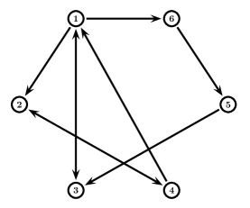
Figure 1: A strongly connected directed communication graph.

Select $K=-\begin{bmatrix}0.8543&2.5628\end{bmatrix}$ such that $A+BK$ is Hurwitz. Solving the LMI (8) by using the LMI toolbox of Matlab, we obtain a feasible solution $S=\begin{bmatrix}0.5853&-0.5853\\ -0.5853&1.7559\end{bmatrix}.$ The feedback gain matrix of (2) is given by $F=-\begin{bmatrix}2.5628\\ 0.8543\end{bmatrix}$. Let $d_{i}(0)=1$, $i=1,\cdots,6$. Then, with the adaptive protocol (2), the relative states $x_{i}-x_{1}$, $i=2,\cdots,6,$ of the second-order integrators are depicted in Fig. 2. Evidently, consensus is achieved. The adaptive coupling weights $d_{i}$ in (2) are shown in Fig. 3, which converge to finite steady-state values.

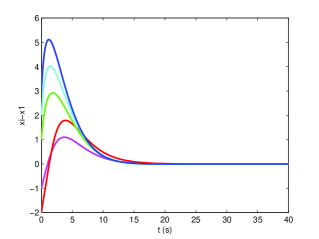
Figure 2: The consensus errors $x_{i}-x_{1}$, $i=2,\cdots,6$ under (2).

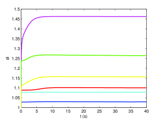
Figure 3: The adaptive gains $d_{i}$ in (2).

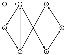
Figure 4: A leader-follower graph containing a directed spanning tree.

Example 2: Consider a network of heterogeneous agents consisting of a leader and several followers. Let the leader be a nonlinear Chua’s circuit, whose dynamics in the dimensionless form are given by [38]

$$\dot{x}_{0} =Ax_{0}+Bf_{0}(x_{0}),$$ (65)

where

$$x_{0} =\left[\begin{matrix}x_{01}\\ x_{02}\\ x_{03}\end{matrix}\right],A=\left[\begin{matrix}-a(m_{0}^{1}+1)&a&0\\ 1&-1&1\\ 0&-b&0\end{matrix}\right],B=\left[\begin{matrix}1\\ 0\\ 0\end{matrix}\right],$$

$$f_{0}(x_{0}) =\frac{a}{2}(m_{0}^{1}-m_{0}^{2})(|x_{01}+1|-|x_{01}-1|),$$

with $a>0$, $b>0$, $m_{0}^{1}<0$, and $m_{0}^{2}<0$ being the parameters of Chua’s circuits. Let $a=9$, $b=18$, $m_{0}^{1}=-\frac{3}{4}$, and $m_{0}^{2}=-\frac{4}{3}$. In this case, the leader displays a double-scroll chaotic attractor [38]. The nonlinear term $f_{0}(x_{0})$ in (65) is regarded as the control input of the leader, which is bounded. The followers are three-order linear systems, described by (1), with $A$ and $B$ given in (65).

The communication graph among the agents are depicted in Fig. 4, where the node indexed by 0 is the leader. For simplicity, it is assumed that the relative state information of neighboring agents is available and the continuous adaptive protocol (62) is used to achieve leader-follower consensus. Solving the linear matrix inequality (16) gives $P=\left[\begin{matrix}0.2403&-0.1467&-0.3444\\ -0.1467&0.1459&0.0332\\ -0.3444&0.0332&2.8821\end{matrix}\right].$ The feedback gain matrices of (62), accordingly, is obtained as $K=-\left[\begin{matrix}2.8843&3.1711&1.5114\end{matrix}\right]$ and $\Gamma=\left[\begin{matrix}8.3194&9.1465&4.3594\\ 9.1465&10.0558&4.7928\\ 4.3594&4.7928&2.2843\end{matrix}\right].$ The initial state of the leader is chosen as $x_{0}(0)=[1,0.8,-1.5]^{T}$ and the initial states of the agents are randomly chosen. Select $\beta=10$, $\kappa=0.05$, and $\varphi_{i}=0.02$ in (62). The state trajectories $x_{i}(t)$ of the agents under (62), designed as above, are depicted in Fig. 5, demonstrating that leader-follower consensus is indeed achieved. The adaptive gains $d_{i}$ in (44) are shown in Fig. 6, which are clearly bounded.

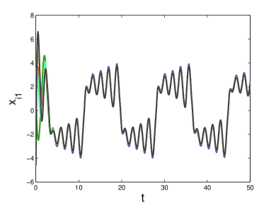
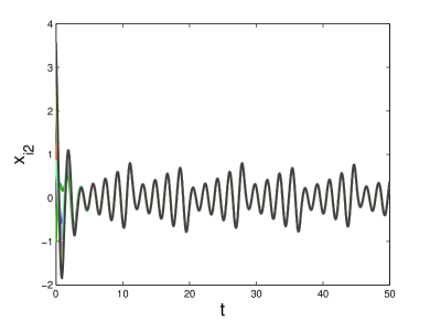
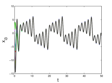
Figure 5: The state trajectories of the leader and the followers under the adaptive protocol (62).

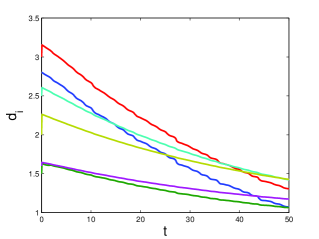
Figure 6: The adaptive gains $d_{i}$ in (62).

VI Conclusion

In this paper, we have addressed the distributed output feedback consensus protocol design problem for linear multi-agent systems with directed graph. One main contribution of this paper is that a new SOD method has been introduced to derive distributed adaptive output feedback consensus protocols, which can solve the leaderless consensus problem for linear multi-agent systems with general directed graphs and the leader-follower consensus problem for the case with a leader of bounded control input.

The adaptive output feedback protocols for the leaderless case are independent of any global information of the communication graph, and thereby are fully distributed. It should be mentioned that the adaptive output feedback protocols for the leader-follower case require the upper bound of the leader’s control input. This issue will be addressed in our future works. Another future direction is to consider the case where the agents are non-introspective, i.e., having access to only the relative output information respect to their neighbors.

References

• [1] W. Ren, R. Beard, and E. Atkins, “Information consensus in multivehicle cooperative control,” IEEE Control Systems Magazine, vol. 27, no. 2, pp. 71–82, 2007.
• [2] G. Antonelli, “Interconnected dynamic systems: An overview on distributed control,” IEEE Control Systems Magazine, vol. 33, no. 1, pp. 76–88, 2013.
• [3] R. Olfati-Saber and R. Murray, “Consensus problems in networks of agents with switching topology and time-delays,” IEEE Transactions on Automatic Control, vol. 49, no. 9, pp. 1520–1533, 2004.
• [4] W. Ren and R. Beard, “Consensus seeking in multiagent systems under dynamically changing interaction topologies,” IEEE Transactions on Automatic Control, vol. 50, no. 5, pp. 655–661, 2005.
• [5] Z. Li, Z. Duan, G. Chen, and L. Huang, “Consensus of multiagent systems and synchronization of complex networks: A unified viewpoint,” IEEE Transactions on Circuits and Systems I: Regular Papers, vol. 57, no. 1, pp. 213–224, 2010.
• [6] Y. Cao, W. Yu, W. Ren, and G. Chen, “An overview of recent progress in the study of distributed multi-agent coordination,” IEEE Transactions on Industrial Informatics, vol. 9, no. 1, pp. 427–438, 2013.
• [7] W. Ren and R. W. Beard, Distributed Consensus in Multi-vehicle Cooperative Control. Communications and Control Engineering, London: Springer-Verlag, 2008.
• [8] Z. Li and Z. Duan, Cooperative Control of Multi-Agent Systems: A Consensus Region Approach. Boca Raton, FL: CRC Press, 2014.
• [9] W. Ren, “On consensus algorithms for double-integrator dynamics,” IEEE Transactions on Automatic Control, vol. 53, no. 6, pp. 1503–1509, 2008.
• [10] W. Ren, K. Moore, and Y. Chen, “High-order and model reference consensus algorithms in cooperative control of multivehicle systems,” ASME Journal of Dynamic Systems, Measurement, and Control, vol. 129, no. 5, pp. 678–688, 2007.
• [11] H. Zhang, F. Lewis, and A. Das, “Optimal design for synchronization of cooperative systems: State feedback, observer, and output feedback,” IEEE Transactions on Automatic Control, vol. 56, no. 8, pp. 1948–1952, 2011.
• [12] J. Seo, H. Shim, and J. Back, “Consensus of high-order linear systems using dynamic output feedback compensator: Low gain approach,” Automatica, vol. 45, no. 11, pp. 2659–2664, 2009.
• [13] W. Yu, G. Chen, M. Cao, and J. Kurths, “Second-order consensus for multiagent systems with directed topologies and nonlinear dynamics,” IEEE Transactions on Systems, Man, and Cybernetics, Part B: Cybernetics, vol. 40, no. 3, pp. 881–891, 2010.
• [14] Z. Li, W. Ren, X. Liu, and L. Xie, “Distributed consensus of linear multi-agent systems with adaptive dynamic protocols,” Automatica, vol. 49, no. 7, pp. 1986–1995, 2013.
• [15] Z. Li, W. Ren, X. Liu, and M. Fu, “Consensus of multi-agent systems with general linear and Lipschitz nonlinear dynamics using distributed adaptive protocols,” IEEE Transactions on Automatic Control, vol. 58, no. 7, pp. 1786–1791, 2013.
• [16] H. Su, G. Chen, X. Wang, and Z. Lin, “Adaptive second-order consensus of networked mobile agents with nonlinear dynamics,” Automatica, vol. 47, no. 2, pp. 368–375, 2011.
• [17] W. Yu, W. Ren, W. X. Zheng, G. Chen, and J. Lü, “Distributed control gains design for consensus in multi-agent systems with second-order nonlinear dynamics,” Automatica, vol. 49, no. 7, pp. 2107–2115, 2013.
• [18] Z. Li, G. Wen, Z. Duan, and W. Ren, “Designing fully distributed consensus protocols for linear multi-agent systems with directed graphs,” IEEE Transactions on Automatic Control, vol. 60, no. 4, pp. 1152–1157, 2015.
• [19] Y. Lv, Z. Li, Z. Duan, and G. Feng, “Novel distributed robust adaptive consensus protocols for linear multi-agent systems with directed graphs and external disturbances,” Automatica, submitted for publication, 2014.
• [20] Z. Li and Z. Ding, “Distributed adaptive consensus and output tracking of unknown linear systems on directed graphs,” Automatica, vol. 55, pp. 12–18, 2015.
• [21] Y. Cao and W. Ren, “Distributed coordinated tracking with reduced interaction via a variable structure approach,” IEEE Transactions on Automatic Control, vol. 57, no. 1, pp. 33–48, 2012.
• [22] J. Mei, W. Ren, and G. Ma, “Distributed coordinated tracking with a dynamic leader for multiple Euler-Lagrange systems,” IEEE Transactions on Automatic Control, vol. 56, no. 6, pp. 1415–1421, 2011.
• [23] J. Mei, W. Ren, and G. Ma, “Distributed containment control for lagrangian networks with parametric uncertainties under a directed graph,” Automatica, vol. 48, no. 4, pp. 653–659, 2012.
• [24] Z. Meng, Z. Lin, and W. Ren, “Leader-follower swarm tracking for networked lagrange systems,” Systems & Control Letters, vol. 61, no. 1, pp. 117–126, 2012.
• [25] Z. Li, X. Liu, W. Ren, and L. Xie, “Distributed tracking control for linear multi-agent systems with a leader of bounded unknown input,” IEEE Transactions on Automatic Control, vol. 58, no. 2, pp. 518–523, 2013.
• [26] J. Mei, W. Ren, and J. Chen, “Consensus of second-order heterogeneous multi-agent systems under a directed graph,” in The 2014 American Control Conference, pp. 802–807, 2014.
• [27] H. Zhang, F. L. Lewis, and Z. Qu, “Lyapunov, adaptive, and optimal design techniques for cooperative systems on directed communication graphs,” IEEE Transactions on Industrial Electronics, vol. 59, no. 7, pp. 3026–3041, 2012.
• [28] D. S. Bernstein, Matrix Mathematics: Theory, Facts, and Formulas. Princeton University Press, 2009.
• [29] J. Slotine and W. Li, Applied nonlinear control. Englewood Cliffs, NJ: Prentice Hall, 1991.
• [30] T. Yang, A. Saberi, A. A. Stoorvogel, and H. F. Grip, “Output consensus for networks of non-identical introspective agents,” in The 50th IEEE Conference on Decision and Control and European Control Conference, pp. 1286–1292, 2011.
• [31] E. Peymani, H. F. Grip, A. Saberi, X. Wang, and T. I. Fossen, “$H_{\infty}$ almost output synchronization for heterogeneous networks of introspective agents under external disturbances,” Automatica, vol. 50, no. 4, pp. 1026–1036, 2014.
• [32] H. Khalil, Nonlinear Systems. Englewood Cliffs, NJ: Prentice Hall, 2002.
• [33] S. E. Tuna, “LQR-based coupling gain for synchronization of linear systems,” arXiv preprint arXiv:0801.3390, 2008.
• [34] K. Young, V. Utkin, and U. Ozguner, “A control engineer’s guide to sliding mode control,” IEEE Transactions on Control Systems Technology, vol. 7, no. 3, pp. 328–342, 1999.
• [35] C. Edwards and S. Spurgeon, Sliding Mode Control: Theory and Applications. London: Taylor & Francis, 1998.
• [36] P. Ioannou and P. Kokotovic, “Instability analysis and improvement of robustness of adaptive control,” Automatica, vol. 20, no. 5, pp. 583–594, 1984.
• [37] S. Tuna, “Conditions for synchronizability in arrays of coupled linear systems,” IEEE Transactions on Automatic Control, vol. 54, no. 10, pp. 2416–2420, 2009.
• [38] R. Madan, Chua’s circuit: a paradigm for chaos. Singapore: World Scientific, 1993.