Lasso based feature selection for malaria risk exposure prediction.

Abstract

In life sciences, the experts generally use empirical knowledge to recode variables, choose interactions and perform selection by classical approach. The aim of this work is to perform automatic learning algorithm for variables selection which can lead to know if experts can be help in they decision or simply replaced by the machine and improve they knowledge and results. The Lasso method can detect the optimal subset of variables for estimation and prediction under some conditions. In this paper, we propose a novel approach which uses automatically all variables available and all interactions. By a double cross-validation combine with Lasso, we select a best subset of variables and with GLM through a simple cross-validation perform predictions. The algorithm assures the stability and the the consistency of estimators.

1 Introduction

Malaria is endemic in developing countries, mainly in sub-Saharan Africa. It is the main cause of mortality especially for children under five years of age in Africa [13]. Generally, cohort studies take place in endemic areas for characterizing the malaria risk. These cohorts studies are on newborn babies and pregnant women. They are introduced to know about the immunity of newborn face to malaria and the construction of this immunity. They also help to know the determinants implicated in the appearance of first malaria infections on the newborn. The distribution of the main vector of malaria (anopheles) and the exposure to malaria risk are spatiotemporal and different at small scale (house level) [2]. Generally the experts in medicine and epidemiology, use they empirical knowledge on phenomenon in the process of data analysis. Some variables are automatically recoded because in numeric form, they are not interpretable [2] and interactions are chosen. Classical variables selection methods are wrapper (forward, backward, stepwise, etc.), embedded, filter and ranking. All details on theses methods are described in [7]. The goal of wrapper method is to select subset of variables with a low prediction error. The wrapper algorithm is improved by Structural wrapper to obtain a sequence of nested subset of feature for optimality is developed in [1]. In practice, classical method of features selection are practically unfeasible in high dimension because the number of features subsets given by ($2^{p}$) where $p$ is the number of features, increases. The Lasso method proposed by Tibshirani [12] is a regularized estimation approach for regression models that uses an $L_{1}$-norm and constrains the regression coefficients. The Lasso method minimize the likelihood $L(\beta)$ or the log-likelihood $l(\beta)$. The results of this method is that all coefficients are shrunken toward zero and some are set exactly to zero. Many studies [4], [6], [11], [14] have improved the original Lasso method. The Generalized Linear Model (GLM) combined with the Lasso, penalize the log-likelihood of the GLM and constrains the $L_{1}$ or $L_{2}$ or ($L_{1}$+$L_{2}$)-norm of the regression coefficients to be inferior to some parameter known as tuning or regularizing parameter [6], [14]. The usage of penalization technique to select variables in generalized models is at embryonic stage. Most of the algorithms implemented in our work are based on [9], [6], [14]. According to the nature of the target variable, family of models used for feature selection, estimation and prediction are generally linear models, generalized models, mixed models, generalized mixed models, multilevel modeling [2]. It is also well known that cross-validation may lead to overfitting[3] and one alternative solution is $precentile-cv$ [10]. The results will be compared to the results of those of the reference method (B-GLM) which uses a backward procedure combine with a GLM [2]

2 Methodology

2.1 Data collection and variables

The study area was conducted in Tori-Bossito a district of Republic of Bénin, between July 2007 and July 2009. The study area (season, vegetation), the methodology of mosquito collection and identfication, the environnement and behavioral data are described in [2]. The dependent variable was the number of Anopheles collected in a house over the three nights of each catch, and the explanatory variables were the environmental factors, i.e. the mean rainfall between two catches (Rainfall), the number of rainy days in the ten days before the catch (RainyDN10), the season during which the catch was carried out (Season), the type of soil 100 meters around the house (Soil), the presence of constructions within 100 meters of the house (Works), the presence of abandoned tools within 100 meters of the house (Tools), the presence of a watercourse within 500 meters of the house (Watercourse), the type of vegetation 100 meters around the house (NDVI), the type of roof (Roof), the number of windows (Windows), the ownership of bed nets (Bed nets), the use of insect repellent and the number of inhabitants in the house (Repellent), see more details in [2], the number of rainy days during the three days of one survey (RainyDN). In the previous work [2], a second type of variables are obtained by recoding the original explanatory variables one based of the knowledge of experts in entomology and medicine. The Original and recoded variables are described in tables (6,7).
Four type of combination of these variables have been used. The firs is only the original variables, the second the original variables with village as fixed effect, the third is recoded variables and the last is the recoded variables with village as fixed effect.

2.2 Models

The algorithm implemented uses GLM-Lasso to detect the entire paths of the variables, in order to detect all changes in the process of regularization. This regularization consist on penalizing the likelihood of the GLMs by adding a penalty term

$$\mathcal{P}(\lambda)=\lambda\sum_{i=1}^{p}{\lvert\beta_{i}\lvert}$$ (1)

with $\lambda\geq 0$.
Then the log-likelihood penalized is :

$$l_{pen}(\beta|Y)=l_{GLM}(\beta|Y)+\mathcal{P}(\lambda)$$ (2)

The penalty problem is reduce to :

$$\hat{\beta}=Arg\max_{\beta}{\left[l_{GLM}(\beta|Y)+\mathcal{P}(\lambda)\right]}$$ (3)

The choice of the regularizing parameter lambda is done by minimizing a score function. In practice, this equation doesn’t have exact numerical solution. It can be used the combination of Laplace approximation, the Newton-Raphson method or the Fisher scoring to solve it. This procedure is used at each learning step.
One of the power of the Lasso is to shrink some coefficients toward to zero and the other to exactly zero. When the regularizing parameter $\lambda$ exceeds certain threshold $(\lambda_{max})$, the intercept is the only non-zero coefficient [12]. For two different values of the regularizing parameter $\lambda$ and $\lambda^{\prime}$ inferior to $\lambda_{max}$, let $\beta$ and $\beta^{\prime}$ be the vectors of fixed coefficients respectively associated to $\lambda$ and $\lambda^{\prime}$, $\beta\neq\beta^{\prime}$ [4, 12]. Then let us define the function

$$Q:\begin{array}[]{l}\lambda_{i}\longmapsto\hat{\beta}_{i}\cr\end{array}$$

$\lambda_{i}\;\in\;\left[0,\lambda_{max}\right]$, $\hat{\beta}_{i}$ is the vector of coefficients $\hat{\beta}_{i}=(\hat{\beta}_{i1},\hat{\beta}_{i2},..,\hat{\beta}_{ip})$, $p$ is the number of coefficients in the model. The parameter $\lambda$ is considered as discreet then $\lambda_{i}\;\in\;\{\lambda_{0},\lambda_{1},...,\lambda_{max}\}$. Because the lasso coefficients are biased, GLM is used to debiased estimators and makes predictions. Under matrix shape, GLM model is

$$g[E(Y|\beta)]=X\beta$$ (4)

where $(Y|,\beta)$ follow a Poisson distribution of parameter $E(Y|\beta)$,
$n$  is the number of observations, $X$ the $n\times\,(p+1)$-dimension matrix of co-variables (environmental variables), $\beta$ is a $(p+1)$-vector of fixed parameters including the intercept, $Y$ is the vector of the target variable.

$$(Y|X=x)\sim\mathcal{P}(\lambda);\;\;\mbox{where}\;\;\lambda=e^{x\beta}$$ (5)

Then

$$\mathbb{P}((Y=y_{i}|X=x))=\frac{e^{(x\beta)^{y_{i}}}}{(y_{i})!}\times e^{-e^{x\beta}}$$ (6)

With $Z_{i}=(Y=y_{i}|X=x)$, the likelihood on $n$ observations can defined as

$$L(Z_{1},\ldots,Z_{n})=\prod_{i=1}^{n}\frac{e^{(x\beta)^{y_{i}}}}{(y_{i})!}\times e^{-e^{x\beta}}$$ (7)

And the log-likelihood is

$$\mathcal{L}(Z_{1},\ldots,Z_{n}) = \log\left(\prod_{i=1}^{n}\frac{e^{(x\beta)^{y_{i}}}}{(y_{i})!}\times e^{-e^{x\beta}}\right)$$ (8)

$$= -\sum^{n}_{i=1}\log((y_{i})!)+\sum^{n}_{i=1}y_{i}(x\beta)-e^{(x\beta)}$$ (9)

$y_{i}$ don’t depend on $\lambda$ then

$$\mathcal{L}(Z_{1},\ldots,Z_{n})=Cste+\sum^{n}_{i=1}y_{i}(x\beta)-e^{(x\beta)}\quad\mbox{where}\quad Cste=-\sum^{n}_{i=1}\log((y_{i})!)$$ (10)

2.3 Leave One Level Out Double Cross-Validation (LOLO-DCV)

This algorithm is a double cross-validation with two levels. Its aim is to compute a second cross-validation (CV2) for prediction at each step of learning of a first cross-validation (CV1). The predictors obtained with (CV2) are consistent for prediction on the test set for (CV1). This algorithm run like described in Algorithm (1).

Algorithme 1 LOLO-DCV

1. The data are separated in $N$-folds

2. A each step of the first level

   1. The folds are regrouped in two part : $E_{A}$ and $E_{T}$, $E_{A}$ : the learning set which contained the observations of $(N-1)$-folds,
      $E_{T}$ : the test set, contained the observations of the last fold.

   2. Hold-out $E_{T}$

   3. The second level of cross-validation

      1. A full cross validation is compute on $E_{A}$

      2. The two regularizing parameters ”lambda.min” and lambda.1se” are got back.

      3. The coefficients of actives variables (variables with non-zero coefficient) associated to these two parameters are debiased

      4. Prediction are performed using a glm model on $E_{T}$

      5. The presence $\mathcal{P}(X_{i})$ of each variable is determined

3. The step (2c) is repeated until predictions is performed for all observations.

LOLO-DCV uses a score of cross validation defined like:

$$Score(\lambda_{i})=Deviance(\lambda_{i})=2\times\left(\mathcal{L}_{(sat)}-\mathcal{L}_{(\lambda_{i})}\right)$$ (11)

Where $\mathcal{L}_{(sat)}$is the log-likelihood of saturated model and $\mathcal{L}_{(\lambda_{i})}$ the log-likelihood of the concerned model. For $\lambda=\lambda_{max}$ the model obtained is the null model which contain only the intercept and $\mathcal{L}_{(sat)}=0$, the model which adjust perfectly data. Then

$$Score(\lambda_{max})=Deviance(NULL)=-2\times\left(\mathcal{L}_{\lambda_{max}}\right)$$ (12)

$$Score(\lambda_{i}) = -2\times\left(\mathcal{L}_{(\lambda_{i})}\right)$$ (13)

$$= -2\left[\left(Cste+\sum^{n}_{i=1}y_{i}(x\beta)-e^{(x\beta)}\right)\right],\;\;\;k\in\mathbb{R}$$ (14)

$$Score(\lambda_{i}) = 2\left[\left(e^{(x\beta)}-\sum^{n}_{i=1}y_{i}(x\beta)\right)\right]+K,\;\;\;K\in\mathbb{R}$$ (15)

To minimize the score is reduced to minimize the quantity $\left(\sum^{n}_{i=1}y_{i}(x\beta)-e^{(x\beta)}\right)$. In gaussian case, the score used is the mean cross-validation error, a vector of length $\lambda$ [5]. Assume that :

$$R=1-\frac{Score(\lambda_{i})}{Score(\lambda_{max})}=1-\alpha$$ (16)

then :

$$Deviance(\lambda_{i})=(1-R)\times Score(\lambda_{max})$$ (17)

We know that $\mathcal{L}_{(sat)}=0$ then $\alpha$ is a log-likelihood ratio between the concerned model and the null model. The optimal value $\lambda.min$ of $\lambda$ is the one minimize the $Score(.)$ function.

$$\lambda.min=Arg\min_{\lambda_{i}}[Score(\lambda_{i})]$$ (18)

For all positive value of $\lambda_{i}$, the score exist and is finite. it shows that the score of cross validation converge. The optimal value of $\lambda_{0j}$ is given by the minimization of the function $Score(.)$.

$$\lambda_{0j}=Arg\min_{\lambda_{i}}[Score(\lambda_{i})]$$ (19)

If $\lambda_{0j}=\lambda_{q}$ then the parameter $lambda.min$ is $lambda.min=\lambda_{q}$ [9], [8]. Let $Std(Score(.))$ the estimate of standard error of $Score(.)$. Suppose

$$\lambda_{0k}=Arg\min_{\lambda_{i}}[Score(\lambda_{i})+Std(Score(\lambda_{i})]$$ (20)

If $\lambda_{0k}=\lambda_{m}$ then the parameter $lambda.1se$ is defined as
$lambda.1se=\lambda_{m}$ [9], [8].

2.4 Prediction power and quality criteria

During the computation of LOLO-DCV :

1. GLM-Lasso is used to trace the trajectories of variables, to detect the high value of the regularizing parameters, and detect changes in the regularization process,

2. a double cross validation is used to select the best subset of variables for prediction based on the score,

3. a GLM is used by the best subset to predict via a simple cross validation.

At last step the prediction accuracy of the method is calculated as average performance across hold-out predictions. For each observation $Y_{i}$, the predicted value is $\hat{Y}_{i}$. We assume that the observed value $Y_{i},1\leq i\leq n$ is really predict by $\hat{Y}_{i}$ if $-0.5\leq Y_{i}-\hat{Y}_{i}\leq 0.5$. The prediction accuracy $P_{a}$ is define by:

$$\left\{\begin{array}[]{l}P_{a}(\hat{Y}_{i})=1\;\;\;\mbox{if}\;\;\;-0.5\leq Y_{i}-\hat{Y}_{i}\leq 0.5\cr P_{a}(\hat{Y}_{i})=0\;\;\;\mbox{elsewhere}.\end{array}\right.$$

This calculation gives the number of good predictions by each method and the power of prediction. The main quality criteria is the prediction power of a model and the other are the mean, the standard deviation, the quadratic risk of prediction. For an any method we have :

Mean $$= \frac{1}{n}\sum_{i=1}^{n}\hat{Y}_{i},\;\;\;\mbox{Deviance}=Score(lambda.min),\;\;\;\mbox{Std}=\sqrt{\mbox{Deviance}}$$

Absolute risk $$= \frac{1}{n}\sum_{i=1}^{n}|Y-\hat{Y}_{i}|,\;\;\mbox{Prediction Power}=\frac{100}{n}\times\#\{i,P_{a}(\hat{Y}_{i})=1,1\leq i\leq n\}$$

where $\#A$ denote the cardinality of $A$

2.5 Frequent variables

Let $X=(X_{1},X_{2},\ldots,X_{p})$ the set of all variables include interactions. A each step $j$ of first level of LOLO-DCV, the Lasso provides the coefficients of all classes of variables and based on this it can determine the presence or the absence of each variable. For any $\lambda$, let define the function ”Presence” of variable like:

$$\left\{\begin{array}[]{l}\mathcal{P}_{j}(X_{i})=1\quad\mbox{if}\quad\beta_{i}(\lambda)\neq 0\cr\mathcal{P}_{j}(X_{i})=0\quad\mbox{elsewhere}.\end{array}\right.$$

where $\beta_{i}(\lambda)$ is a vector of coefficients of $X_{i}$ in the model at the step $j$. For a threshold $s,\quad 1\leq s\leq 100$, the set of frequent variables is

$$\mbox{Var\_freq}(\lambda)=\left\{X_{i},\frac{100}{\max(j)}\times\sum_{l=1}^{max(j)}\mathcal{P}_{j}(X_{i})\geq s\right\}$$ (21)

Notations:
$\mbox{Var freq lambda\_min}=\mbox{Var\_freq}(lambda.min)$
$\mbox{Var freq lambda\_1se}=\mbox{Var\_freq}(lambda.1se)$
LOLO DCV lambda$\_$min denote LOLO-DCV using $\lambda=lambda.min$
LOLO DCV lambda$\_$1se denote LOLO-DCV using $\lambda=lambda.1se$

2.6 interactions between variables

In general experts in epidemiology and medicine decide to choose some interactions according to they knowledge and experience. To avoid this way of making, LOLO-DCV generate automatically all interactions in the full set of explanatory variables used in model. This involves that the number of variables grows exponentially and the classical method of variable selection will failed. LOLO-DCV automatically learn with all variables and all interactions and provides the optimal set of variables for predictions.

3 Results

3.1 Summary of results on prediction accuracy and quality criteria

Table 1: Summary of B-GLM prediction

Method	Mean	Deviance	Std	Absolute risk	Prediction Power (%)
B-GLM	3.75	62.29	7.89	3.88	73.53

Table 2: Summary of original variables

Method	Mean	Deviance	Std	Absolute risk	Prediction Power (%)
LOLO DCV lambda_min	3.75	72.04	8.49	4.48	78.76
LOLO DCV lambda_1se	3.75	72.04	8.49	4.48	78.76
Var freq lambda_min	3.75	68.05	8.25	3.96	74.84
Var freq lambda_1se	3.74	59.28	7.70	3.81	75.98

Table 3: Summary of original variables with village as fixed effect

Method	Mean	Deviance	Std	Absolute risk	Prediction Power (%)
LOLO DCV lambda_min	3.75	72.04	8.49	4.48	78.76
LOLO DCV lambda_1se	3.75	72.04	8.49	4.48	78.76
Var freq lambda_min	3.73	55.70	7.46	3.50	75.00
Var freq lambda_1se	3.74	57.33	7.57	3.63	76.80

Table 4: Summary of recoded variables

Method	Mean	Deviance	Std	Absolute risk	Prediction Power (%)
LOLO DCV lambda_min	3.75	72.04	8.49	4.48	78.76
LOLO DCV lambda_1se	3.75	72.04	8.49	4.48	78.76
Var freq lambda_min	3.75	59.21	7.69	3.84	75.82
Var freq lambda_1se	3.74	59.97	7.74	3.81	73.86

Table 5: Summary of recoded variables with village as fixed effect

Method	Mean	Deviance	Std	Absolute risk	Prediction Power (%)
LOLO DCV lambda_min	3.75	72.04	8.49	4.48	78.76
LOLO DCV lambda_1se	3.75	72.04	8.49	4.48	78.76
Var freq lambda_min	3.73	60.11	7.75	3.87	76.31
Var freq lambda_1se	3.75	59.21	7.69	3.84	75.82

3.2 Quality of estimators and optimal subset variables of prediction

Quality of estimators

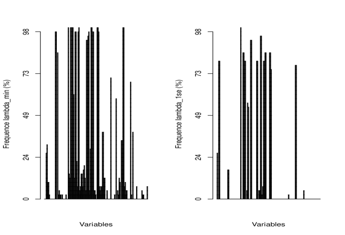
Figure 1: Frequent variables among original variables. At the abscissas ($x_{s}$) are the variables include interactions and at the ordered $(y_{s})$ the percentage of the presence of variables

.

Figure 2: Frequent variables among original variables with village at fixed effect

Recoded variables

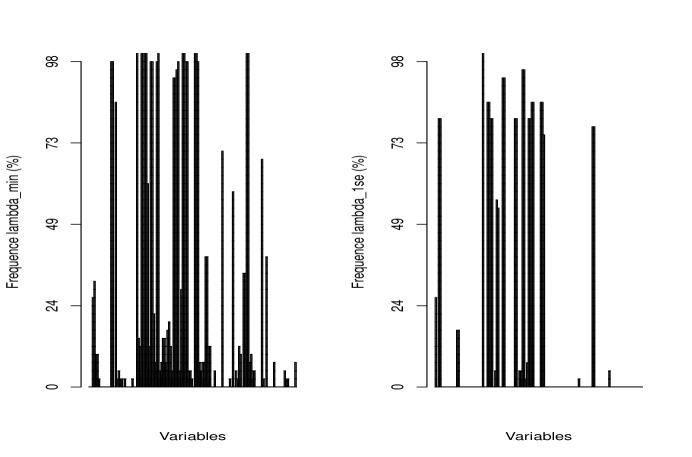
Figure 3: Frequent variables among recoded variables

Figure 4: Frequent variables among recoded variables with village at fixed effect

The best subset of variables selected by each method is:

1. B-GLM prediction:
   Season (season), the number of rainy days during the three days of one survey (RainyDN), mean rainfall between 2 survey (Rainfall), number of rainy days in the 10 days before the survey (RainyDN102), the use of repellent (Repellent), The index of vegetation (NDVI) the interaction between season and NDVI (season:NDVI) [2].

2. LOLO-DCV

   1. Original variables:
      Season and interaction between mean rainfall between 2 survey (season) and the number of rainy days during the three days of one survey (Rainfall:RainyDN).

   2. Original variables with village as fixed effect:
      Season (season) and interaction between number of rainy days in the 10 days before the survey and village (RainyDN10:village).

   3. Recoded variables:
      Season (season) and mean rainfall between 2 survey (RainyDN10).

   4. Recoded variables with village as fixed effect:
      Season (season) and interaction between the number of rainy days during the three days of one survey and presence of work around the site (RainyDN:Works).

LOLO-DCV$\_$lambda$\_$min and LOLO-DCV$\_$lambda$\_$1se achieves exactly the same performance in prediction: Mean, quadratic risk, absolute risk, and prediction power (Table. 2, 3, 4, 5). The mean of predictions of the both methods is approximatively the same with the mean of observations (3.74) which is achieved exactly with frequent variables obtained by lambda$\_$1se selection.
LOLO-DCV shows the Influence of interactions on the target variables. The variability of the score in prediction at village level (high in one the village (Dohinonko)) detect some problems in the data at this village. It is confirmed by the experts. The (Fig. 1, 2 , 3, 4) shows two class of variables, the most frequent and the least frequent. The best Prediction power is with LOLO DCV (78.76) and the one with frequent variable is of LOLO-DCV lambda.1se (76.80), this method also has the same mean in prediction with observations. The number of variables and all interactions is $p=136$, the classical methods will compute $N=2^{136}$ different model before selecting the best subset. Combined with double cross-validation, calculation will be unrealizable because of complexity of algorithm. The strength of LOLO-DCV is the usage of lasso and the two level cross validation. In a relative short time LOLO-DCV detect all feature selected by the B-GLM and some interpretable interactions among them. The (Tables. 1, 2, 3, 4, 5) show that LOLO-DCV is relatively the best in prediction (mean, absolute risk, deviance) and the best with the prediction power. The distribution of the prediction error according to the classes of anopheles shows a high variability for B-GLM and low for the LOLO-DCV. The optimal subset of feature obtained by LOLO-DCV algorithm is approximatively the same at each step. This prove it’s stability. In final the best subset of variables for prediction is variables selected in Original variables with village as fixed effect (2b)

4 Conclusion

Lasso method combined with a GLM uses $L_{1}$ or $L_{2}$ penalization on likelihood to estimate predictors. The usage of Lasso, GLM and cross-validation for features selection is an active area of research in features and variables selection. In this work we propose LOLO-DCV method applied to a real data. The computation time is strongly reduced with the parallelization of the cross-validation loop. The usage of levels for building the folds in cross-validation is important because a random sampling will use all characteristics of all levels and the predictions will be wrong. The experts can easily be helped by the machine in they decision. These results encourage a best exploring of this approach for features selection. Adding random effects at some levels to improve our method is part of our future work possibly by combining the adaptative, group and sparse form of lasso procedure.

Annex

Description of originales variables

Table 6: Originale variables.

Variables	Nature	Number of modalities	Modalities
Repellent	Nominal	2	Yes/ No
Bed-net	Nominal	2	Yes/ No
Type of roof	Nominal	2	Tole/ Paille
Ustensils	Nominal	2	Yes/ No
Presence of constructions	Nominal	2	Yes/ No
Type of soil	Nominal	2	Humid/ Dry
Water course	Nominal	2	Yes/ No
Majority Class	Nominal	3	1/4/7
Season	Nominal	4	1/2/3/4
Village	Nominal	9
House	Nominal	41
Rainy days before mission	Numeric	Discrete	0/2/$\cdots$/9
Rainy days during mission	Numeric	Discrete	0/1/$\cdots$/3
Fragmentation Index	Numeric	Discrete	26/$\cdots$/71
Openings	Numeric	Discrete	1/$\cdots$/5
Number of inhabitants	Numeric	Discrete	1/$\cdots$/8
Mean rainfall	Numeric	Continue	0/$\cdots$/82
Vegetation	Numeric	Continue	115.2/$\cdots$/ 159.5
Total Mosquitoes	Numeric	Discrete	0/$\cdots$/481
Total Anopheles	Numeric	Discrete	0/$\cdots$/87
Anopheles infected	Numeric	Discrete	0/$\cdots$/9

Description of recoded variables

Table 7: Recoded variables. Variables with star are recoded.

Variables	Nature	Number of modalities	Modalities
Repellent	Nominal	2	Yes/ No
Bed-net	Nominal	2	Yes/ No
Type of roof	Nominal	2	Tole/ Paille
Utensils	Nominal	2	Yes/ No
Presence of constructions	Nominal	2	Yes/ No
Type of soil	Nominal	2	Humid/ Dry
Water course	Nominal	2	Yes/ No
Majority class ∗	Nominal	3	1/2/3
Season	Nominal	4	1/2/3/4
Village∗	Nominal	9
House ∗	Nominal	41
Rainy days before mission ∗	Nominal	3	Quartile
Rainy days during mission	Numeric	Discrete	0/1/$\cdots$/3
Fragmentation index ∗	Nominal	4	Quartile
Openings∗	Nominal	4	Quartile
Nber of inhabitants ∗	Nominal	3	Quartile
Mean rainfall ∗	Nominal	4	Quartile
Vegetation∗	Nominal	4	Quartile
Total Mosquitoes	Numeric	Discrete	0/$\cdots$/481
Total Anopheles	Numeric	Discrete	0/$\cdots$/87
Anopheles infected	Numeric	Discrete	0/$\cdots$/9

References

- [1] Bontempi, G.: Structural feature selection for wrapper methods. In: ESANN 2005, 13th European Symposium on Artificial Neural Networks, Bruges, Belgium, April 27-29, 2005, Proceedings. pp. 405–410 (2005), https://www.elen.ucl.ac.be/Proceedings/esann/esannpdf/es2005-97.pdf
- [2] Cottrell, G., Kouwayè, B., Pierrat, C., le Port, A., Bouraïma, A., Fonton, N., Hounkonnou, M.N., Massougbodji, A., Corbel, V., Garcia, A.: Modeling the influence of local environmental factors on malaria transmission in benin and its implications for cohort study. PlosOne 7, 8 (2012)
- [3] De Bradanter, J., Pelckmans, K., Suykens, J.A.K., Vandewalle, J., De Moor, B.: Robust cross validation score function with application to weigthed least squares support vector machine function estimation (2003), katholieke Universiteit Leuven, departement of electrical engineering, ESAT-SISTA
- [4] Efron, B., Hastie, T., Johnstone, I., Tibshirani, R.: Least angle regression. The Annals of statistics 32(2), 407–499 (2005)
- [5] Friedman, J., Hastie, T., Tibshirani, R.: Regularization paths for generalized linear models via coordinate descent. Journal of Statistical Software 33(1), 1–22 (2010), http://www.jstatsoft.org/v33/i01/
- [6] Goeman, J.J.: L1 penalized estimation in the cox proportional hazards model. Biometrical Journal 52(1), 70–84 (2010)
- [7] Guyon, I.: An introduction to variable and feature selection. Journal of Machine Learning Research 3, 1157–1182 (2003)
- [8] Hastie, T., Tibshirani, R., Friedman, J.: The Elements of Statistical Learning Data mining, Inference, Prediction. Springer, second edn. (2009)
- [9] J. Friedman, T. Hastie, N.S., Tibshirani, R.: Lasso and elastic-net regularized generalized linear models (2015), http://www.jstatsoft.org/v33/i01/ R CRAN
- [10] Ng, A.Y.: Preventing ”overfitting” of cross-validation data. In: Proceedings of the Fourteenth International Conference on Machine Learning. pp. 245–253. ICML ’97, Morgan Kaufmann Publishers Inc., San Francisco, CA, USA (1997), http://dl.acm.org/citation.cfm?id=645526.657119
- [11] Osborne, M., Presnell, B., Turlach, B.: A new approach to variable selection in least squares problems. IMA Journal of Numerocal Analysis 20, 389–403 (2000)
- [12] Tibshirani, R.: Regression shrinkage and selection via the lasso. Journal of the Royal Statistical Society. Series B (Methodological) pp. 267–288 (1996)
- [13] WHO: World health organisation, world malaria report 2013, world global malaria programme. WHO Library Cataloguing-in-Publication Data p. 248 (2013)
- [14] Zou, H., Hastie, T.: Regularization and variable selection via the elastic net. Journal of the Royal Statistical Society: Series B (Statistical Methodology) 67(2), 301–320 (2005)