Factorizing LambdaMART for cold start recommendations

Abstract

Recommendation systems often rely on point-wise loss metrics such as the mean squared error. However, in real recommendation settings only few items are presented to a user. This observation has recently encouraged the use of rank-based metrics. LambdaMART is the state-of-the-art algorithm in learning to rank which relies on such a metric. Despite its success it does not have a principled regularization mechanism relying in empirical approaches to control model complexity leaving it thus prone to overfitting.

Motivated by the fact that very often the users’ and items’ descriptions as well as the preference behavior can be well summarized by a small number of hidden factors, we propose a novel algorithm, LambdaMART Matrix Factorization (LambdaMART-MF), that learns a low rank latent representation of users and items using gradient boosted trees. The algorithm factorizes lambdaMART by defining relevance scores as the inner product of the learned representations of the users and items. The low rank is essentially a model complexity controller; on top of it we propose additional regularizers to constraint the learned latent representations that reflect the user and item manifolds as these are defined by their original feature based descriptors and the preference behavior. Finally we also propose to use a weighted variant of NDCG to reduce the penalty for similar items with large rating discrepancy.

We experiment on two very different recommendation datasets, meta-mining and movies-users, and evaluate the performance of LambdaMART-MF, with and without regularization, in the cold start setting as well as in the simpler matrix completion setting. In both cases it outperforms in a significant manner current state of the art algorithms.

1 Introduction

Most recommendation algorithms minimize a point-wise loss function such as the mean squared error or the mean average error between the predicted and the true user preferences. For instance in matrix factorization, a learning paradigm very popular in recommendation problems, state-of-the-art approaches such as [12, 1, 2] minimize the squared error between the inner product of the learned low-rank representations of users and items and the respective true preference scores. Such cost functions are clearly not appropriate for recommendation problems since what matters there is the rank order of the preference scores and not their absolute values, i.e. items that are very often top ranked should be highly recommended. It is only recently that recommendation methods have started using ranking-based loss functions in their optimization problems. Cofirank [13], a collaborative ranking algorithm, does maximum-margin matrix factorization by optimizing an upper bound of NDCG measure, a ranking-based loss function. However, like many recommendation algorithms, it cannot address the cold start problem, i.e. it cannot recommend new items to new users.

In preference learning [8] we learn the preference order of documents for a given query. Preference learning algorithm are used extensively in search engines and IR systems and optimize ranking-based loss functions such as NDCG. Probably the best known example of such algorithms is LambdaMART, [4], the state-of-the-art learning to rank algorithm. Its success is due to its ability to model preference orders using features describing side-information of the query-document pairs in a very flexible manner. Nevertheless it is prone to overfitting because it does not come with a rigorous regularization formalization and relies instead on rather empirical approaches to protect against it, such as validation error, early stopping, restricting the size of the base level trees etc.

In this paper we develop a new recommendation algorithm with an emphasis on the cold start problem and the exploitation of available side-information on users and items. Our algorithm can be thought of as a variant of LambdaMART in which instead of directly learning the user-item preferences, as LambdaMART does, we first learn low rank latent factors that describe the users and the items and use them to compute the user-item preference scores; essentially our algorithm does a low-rank matrix factorization of the preferences matrix. Moreover we provide additional data-based regularizers for the learned latent representations of the users and items that reflect the user and item manifolds as they are established from their side-information as well as from the preference matrix. We evaluate the performance of our algorithm on two very different recommendation applications and compare its performance to a number of baselines, amongst which LambdaMART, and demonstrate very significant performance improvements.

2 Preliminaries

We are given a (sparse) preference matrix, ${\mathbf{Y}}$, of size $n\times m$. The $(i,j)$ non-missing entry of ${\mathbf{Y}}$ represents the preference score of the $i$th user for the $j$th item in recommendation problems or the relevance score of the $j$th document for the $i$th query in learning to rank problems, the larger the value of the $(i,j)$ entry the larger the relevance or preference is. In addition to the preference matrix, we also have the descriptions of the users and items. We denote by $\boldsymbol{c}_{i}=(c_{i1},\dots,c_{id})^{\text{T}}\in\mathbb{R}^{d}$, the $d$-dimensional description of the $i$th user, and by $\mathbf{C}$ the $n\times d$ user description matrix, the $i$th row of which is given by the $\boldsymbol{c}_{i}^{T}$. Similarly, we denote by $\boldsymbol{d}_{j}=(d_{j1},\dots,d_{jl})^{\text{T}}\in\mathbb{R}^{l}$, the $l$-dimensional description of the $j$th item and by $\mathbf{D}$ the $m\times l$ item description matrix, the $j$th row of which is given by the $\mathbf{d}_{j}^{T}$.

As already mentioned when recommending an item to a user we only care about the rank order of $y_{ij}$ and not the actual preference score value $y_{ij}$. Thus in principle a preference learning algorithm does not need to predict the exact value of $y_{ij}$ but only its rank order as this induced by the preference vector $\boldsymbol{y}$. We will denote by $\boldsymbol{r}_{\boldsymbol{c}_{i}}$ the target rank vector of the $i$th user. We construct $\boldsymbol{r}_{\boldsymbol{c}_{i}}$ by ordering in a decreasing manner the $i$th user’s non-missing preference scores over the items; its $k$th entry, $\boldsymbol{r}_{{\boldsymbol{c}_{i}}k}$, is the rank of the $k$th non-missing preference score, with the highest preference score having a rank of one. In the inverse problem, i.e. matching users to items, we will denote by $\boldsymbol{r}_{\boldsymbol{d}_{j}}$ the target rank vector of the $j$th item, given by ordering the $j$th item’s non-missing relevance scores for the users.

2.1 Evaluation Metric

In real applications of preference learning, such as recommendation, information retrieval, etc, only a few top-ranked items are finally shown to the users. As a result appropriate evaluation measures for preference learning focus on the correctness of the top-ranked items. One such, very often used, metric is the Discounted Cumulative Gain (DCG)[10], which is defined as follows:

$$\text{DCG}(\boldsymbol{r},\boldsymbol{y})@k = \sum_{i=1}^{M}\frac{2^{y_{i}}-1}{\log_{2}(r_{i}+1)}I(r_{i}\leq k)$$ (1)

where $k$ is the truncation level at which DCG is computed and $I$ is the indicator function which returns $1$ if its argument holds otherwise $0$. $\boldsymbol{y}$ is the $m$ dimensional ground truth relevance vector and $\boldsymbol{r}$ is a rank vector that we will learn. The DCG score measures the match between the given rank vector $\boldsymbol{r}$ and the rank vector of the relevance score vector $\boldsymbol{y}$. It is easy to check that if the rank vector $\boldsymbol{r}$ correctly preserves the order induced by $\boldsymbol{y}$ then the DCG score will achieve its maximum. Due to the log in the denominator the DCG score will incur larger penalties when misplacing top items compared to than low end items, emphasizing like that the correctness of top items.

Since the DCG score also depends on the length of the relevance vector $\boldsymbol{y}$, it is often normalized with respect to its maximum score, resulting to what is known as the Normalized DCG (NDCG), defined as:

$$\text{NDCG}(\boldsymbol{y},\hat{\boldsymbol{y}})@k = \frac{\text{DCG}(r(\hat{\boldsymbol{y}}),\boldsymbol{y})@k}{\text{DCG}(r(\boldsymbol{y}),\boldsymbol{y})@k}$$ (2)

$r(\cdot)$ is a rank function that outputs the rank vector, in decreasing order, of its input argument vector. Thus the vector $r({\boldsymbol{y}})$ is the rank vector of the ground truth relevance vector $\boldsymbol{y}$ and $r(\hat{\boldsymbol{y}})$ is the rank vector of the predicted relevance vector $\hat{\boldsymbol{y}}$ provided by the learned model. With normalization, the value of NDCG ranges from $0$ to $1$, the larger the better. In this paper, we will also use this metric as our evaluation metric.

2.2 LambdaMART

The main difficulty in learning preferences is that rank functions are not continuous and have combinatorial complexity. Thus most often instead of the rank of the preference scores the pairwise order constraints over the items’ preferences are used. LambdaMART is one of the most popular algorithms for preference learning which follows exactly this idea, [4]. Its optimization problem relies on a distance distribution measure, cross entropy, between a learned distribution that gives the probability that item $j$ is more relevant than item $k$ from the true distribution which has a probability mass of one if item $i$ is really more relevant than item $j$ and zero otherwise. The final loss function of LambdaMart defined over all users $i$ and overall the respective pairwise preferences for items $j$, $k$, is given by:

$$\mathcal{L}(\mathbf{Y},\hat{\mathbf{Y}})=\sum^{n}_{i=1}\sum_{\{jk\}\in Z}|\Delta NDCG^{i}_{jk}|\log(1+e^{-\sigma(\hat{y}_{ij}-\hat{y}_{ik})})$$ (3)

where $Z$ is the set of all possible pairwise preference constraints such that in the ground truth relevance vector holds $y_{ij}>y_{ik}$, and $\Delta NDCG^{i}_{jk}$ is given by:

$$\Delta NDCG^{i}_{jk}=NDCG(r(\boldsymbol{y}_{i}),r(\hat{\boldsymbol{y}}_{i}))-NDCG(r(\boldsymbol{y}^{jk}_{i}),r(\hat{\boldsymbol{y}}_{i}))$$

where $\boldsymbol{y}^{jk}_{i}$ is the same as the ground truth relevance vector $\boldsymbol{y}_{i}$ except that the values of $y_{ij}$ and $y_{ik}$ are swapped. This is also equal to the NDCG difference that we get if we swap the $\hat{y}_{ij}$, $\hat{y}_{ik}$, estimates. Thus the overall loss function of LambdaMART eq 3 is the sum of the logistic losses on all pairwise preference constraints weighted by the respective NDCG differences. Since the NDCG measure penalizes heavily the error on the top items, the loss function of LambdaMART has also the same property. LambdaMART minimizes its loss function with respect to all $\hat{y}_{ij},\hat{y}_{ik}$, and its optimization problem is:

$$\min_{\hat{\mathbf{Y}}}\mathcal{L}(\mathbf{Y},\hat{\mathbf{Y}})$$ (4)

[14] have shown empiricially that solving this problem also optimizes the NDCG metric of the learned model. The partial derivative of LambdaMART’s loss function with respect to the estimated scores $\hat{y}_{ij}$ is

$$\frac{\partial\mathcal{L}(\mathbf{Y},\hat{\mathbf{Y}})}{\partial\hat{y}_{ij}}=\lambda^{i}_{j}=\sum_{\{k|jk\}\in Z}\lambda^{i}_{jk}-\sum_{\{k|kj\}\in Z}\lambda^{i}_{kj}$$ (5)

and $\lambda^{i}_{jk}$ is given by:

$$\lambda^{i}_{jk}=\frac{-\sigma}{1+e^{\sigma(\hat{y}_{ij}-\hat{y}_{ik})}}|\bigtriangleup_{NDCG}(\hat{y}_{ij},\hat{y}_{ik})|$$ (6)

With a slight abuse of notation below we will write $\frac{\partial\mathcal{L}(y_{ij},\hat{y_{ij}})}{\partial\hat{y}_{ij}}$ instead of $\frac{\partial\mathcal{L}(\mathbf{Y},\hat{\mathbf{Y}})}{\partial\hat{y}_{ij}}$, to make explicit the dependence of the partial derivative only on $y_{ij},\hat{y}_{ij}$ due to the linearity of $\mathcal{L}(\mathbf{Y},\hat{\mathbf{Y}})$.

LambdaMART uses Multiple Additive Regression Trees (MART) [7] to solve its optimization problem. It does so through a gradient descent in the functional space that generates preference scores from item and user descriptions, i.e. $\hat{y}_{ij}=f(\boldsymbol{c}_{i},\boldsymbol{d}_{j})$, where the update of the preference scores at the $t$ step of the gradient descent is given by:

$$\hat{y}^{(t)}_{ij}=\hat{y}^{(t-1)}_{ij}-\eta\frac{\partial\mathcal{L}(y_{ij},\hat{y}^{(t-1)}_{ij})}{\partial\hat{y}^{(t-1)}_{ij}}$$ (7)

or equivalently:

$$f^{(t)}(\boldsymbol{c}_{i},\boldsymbol{d}_{j})=f^{(t-1)}(\boldsymbol{c}_{i},\boldsymbol{d}_{j})-\eta\frac{\partial\mathcal{L}(y_{ij},f^{(t-1)}(\boldsymbol{c}_{i},\boldsymbol{d}_{j}))}{\partial f^{(t-1)}(\boldsymbol{c}_{i},\boldsymbol{d}_{j})}$$ (8)

where $\eta$ is the learning rate. We terminate the gradient descent when we reach a given number of iterations $T$ or when the validation loss NDCG starts to increase. We approximate the derivative $\frac{\partial\mathcal{L}(y_{ij},\hat{y}^{(t-1)}_{ij})}{\partial\hat{y}^{(t-1)}_{ij}}$ by learning at each step $t$ a regression tree $h^{(t)}(\boldsymbol{c},\boldsymbol{d})$ that fits it by minimizing the sum of squared errors. Thus at each update step we have

$$f^{(t)}(\boldsymbol{c}_{i},\boldsymbol{d}_{j})=f^{(t-1)}(\boldsymbol{c}_{i},\boldsymbol{d}_{j})+\eta h^{(t)}(\boldsymbol{c}_{i},\boldsymbol{d}_{j})$$ (9)

which if we denote by $\gamma_{tk}$ the prediction of the $k$th terminal node of the $h^{(t)}$ tree and by $h_{tk}$ the respective partition of the input space, we can rewrite as:

$$f^{(t)}(\boldsymbol{c}_{i},\boldsymbol{d}_{j})=f^{(t-1)}(\boldsymbol{c}_{i},\boldsymbol{d}_{j})+\eta\gamma_{tk}I((\boldsymbol{c},\boldsymbol{d})\in h_{tk})$$ (10)

we can further optimize over the $\gamma_{tk}$ values to minimize the loss function of eq 3 over the instances of each $h_{tk}$ partition using Newton’s approximation. The final preference estimation function is given by:

$$\hat{y}=f(\boldsymbol{c},\boldsymbol{d})=\sum_{t=1}^{T}\eta h^{(t)}(\boldsymbol{c},\boldsymbol{d})$$ (11)

or

$$\hat{y}=f(\boldsymbol{c},\boldsymbol{d})=\sum^{T}_{t=1}\eta\gamma_{tk}I((\boldsymbol{c},\boldsymbol{d})\in h_{tk})$$ (12)

LambdaMart is a very effective algorithm for learning to rank problems, see e.g [5, 6]. It learns non-linear relevance scores, $\hat{y}_{ij}$, using gradient boosted regression trees. The number of the parameters it fits is given by the number of available preference scores (this is typically some fraction of $n\times m$); there is no regularization on them to prevent overfitting. The only protection against overfitting can come from rather empirical approaches such as constraining the size of the regression trees or by selecting learning rate $\eta$.

3 Factorized Lambda-MART

In order to address the rather ad-hoc approach of LambdaMART to prevent overfitting we propose here a factorized variant of it that does regularization in a principled manner. Motivated by the fact that very often the users’ and the items’ descriptions and their preference relations can be well summarized by a small number of hidden factors we learn a low rank hidden representation of users and items using gradient boosted trees, MART. We define the relevance score as the inner product of the new representation of the users and items which has the additional advantage of introducing low rank structural regularization in the learned preference matrix.

Concretely, we define the relevance score of the $i$th user and $j$th item by $\hat{y}_{ij}=\boldsymbol{u}_{i}^{\text{T}}\boldsymbol{v}_{j}$, where $\mathbf{u}_{i}$ and $\mathbf{v}_{j}$ are the $r$-dimensional user and item latent descriptors. We denote by $\mathbf{U}:n\times r$ and $\mathbf{V}:m\times r$ the new representation matrices of users and items. The dimensionality of $r$ is a small number, $r<<\min(n,m)$. The loss function of eq 3 now becomes:

$$\mathcal{L}_{MF}(\mathbf{Y},\hat{\mathbf{U}},\hat{\mathbf{V}})=\sum_{i=1}^{n}\sum_{\{jk\}\in Z}|\bigtriangleup_{NDCG}|\log(1+e^{-\sigma(\hat{\boldsymbol{u}}_{i}(\hat{\boldsymbol{v}}_{j}-\hat{\boldsymbol{v}}_{k}))})$$ (13)

The partial derivatives of this lost function with respect to $\hat{\boldsymbol{u}}_{i},\hat{\boldsymbol{v}}_{j}$, are given by:

$$\frac{\partial\mathcal{L}_{MF}(\mathbf{Y},\hat{\mathbf{U}},\hat{\mathbf{V}})}{\partial\hat{\boldsymbol{u}}_{i}}=\sum_{j=1}^{m}\frac{\partial\mathcal{L}_{MF}(\mathbf{Y},\hat{\mathbf{Y}})}{\partial\hat{y}_{ij}}\frac{\partial\hat{y}_{ij}}{\partial\hat{\boldsymbol{u}}_{i}}=\sum_{j=1}^{m}\lambda^{i}_{j}\frac{\partial\hat{y}_{ij}}{\partial\hat{\boldsymbol{u}}_{i}}$$ (14)

$$\frac{\partial\mathcal{L}_{MF}(\mathbf{Y},\hat{\mathbf{U}},\hat{\mathbf{V}})}{\partial\hat{\boldsymbol{v}_{j}}}=\sum_{i=1}^{n}\frac{\partial\mathcal{L}_{MF}(\mathbf{Y},\hat{\mathbf{Y}})}{\partial\hat{y}_{ij}}\frac{\partial\hat{y}_{ij}}{\partial\hat{\boldsymbol{v}}_{i}}=\sum_{i=1}^{n}\lambda^{i}_{j}\frac{\partial\hat{y}_{ij}}{\partial\boldsymbol{v}_{j}}$$ (15)

Note that the formulation we give in equation 13 is very similar to those used in matrix factorization algorithms. Existing matrix factorization algorithms used in collaborative filtering recommendation learn the low-rank representation of users and items in order to complete the sparse preference matrix $\mathbf{Y}$, [12, 13, 1, 2], however these approaches cannot address the cold start problem.

Similar to LambdaMART we will seek a function $f$ that will optimize the $\mathcal{L}_{MF}$ loss function. To do so we will learn functions of the latent profiles of the users and items from their side information. We will factorize $f(\mathbf{c},\mathbf{d})$ by

$$f(\mathbf{c},\mathbf{d})=f_{u}(\mathbf{c})^{\text{T}}f_{v}(\mathbf{d})=\mathbf{u}^{\text{T}}\mathbf{v}=\hat{y}$$

where $f_{u}:\mathcal{C}\rightarrow\mathcal{U}$ is a learned user function that gives us the latent factor representation of user from his/her side information descriptor $\mathbf{c}$; $f_{v}:\mathcal{D}\rightarrow\mathcal{V}$ is the respective function for the items. We will follow the LambdaMART approach described previously and learn an ensemble of trees for each one of the $f_{u}$ and $f_{v}$ functions. Concretely:

$$\hat{\mathbf{u}}_{i} = f_{u}(\mathbf{c}_{i})=\sum_{t=1}^{T}\eta h_{u}^{(t)}(\mathbf{c}_{i})$$ (16)

$$\hat{\mathbf{v}}_{j} = f_{v}(\mathbf{d}_{j})=\sum_{t=1}^{T}\eta h_{v}^{(t)}(\mathbf{d}_{j})$$ (17)

Unlike standard LambdaMART the trees we will learn are multi-output regression trees, predicting the complete latent profile of users or items. Now at each step $t$ of the gradient descent we learn the $h^{(t)}_{u}(\mathbf{c})$ and $h_{v}^{(t)}(\mathbf{d})$ trees that fit the negative of the partial derivatives given at equations 14, 15. We learn the trees by greedily optimizing the sum of squared errors over the over the dimensions of the partial gradients. The $t$ gradient descent step for $\boldsymbol{u}_{i}$ is given by:

$$\boldsymbol{u}_{i}^{(t)}=\mathbf{u}_{i}^{(t-1)}-\sum_{j=1}^{m}\frac{\partial\mathcal{L}_{MF}(\mathbf{Y},\hat{\mathbf{Y}})}{\partial\hat{y}_{ij}}\Big{|}_{\hat{y}_{ij}=\hat{\boldsymbol{u}}^{(t-1)\text{T}}_{i}{\hat{\boldsymbol{v}}_{j}^{(t-1)}}}\frac{\partial\hat{\boldsymbol{u}}_{i}^{\text{T}}{\hat{\boldsymbol{v}}_{j}^{(t-1)}}}{\partial\hat{\boldsymbol{u}}_{i}}$$

and for $\boldsymbol{v}_{j}$ by:

$$\boldsymbol{v}_{j}^{(t)}=\boldsymbol{v}_{j}^{(t-1)}-\sum_{i=1}^{n}\frac{\partial\mathcal{L}_{MF}(\mathbf{Y},\hat{\mathbf{Y}})}{\partial\hat{y}_{ij}}\Big{|}_{\hat{y}_{ij}=\hat{\boldsymbol{u}}_{i}^{(t-1)\text{T}}{\hat{\boldsymbol{v}}_{j}^{(t-1)}}}\frac{\partial\hat{\boldsymbol{u}}_{i}^{(t-1)\text{T}}{\hat{\boldsymbol{v}}_{j}}}{\partial\hat{\boldsymbol{v}}_{j}}$$

The functions of each step are now:

$$f_{\boldsymbol{u}}^{(t)}(\boldsymbol{c})=f_{u}^{(t-1)}(\boldsymbol{c})+\eta h^{(t)}_{u}(\boldsymbol{c})$$ (18)

$$f_{\boldsymbol{v}}^{(t)}(\boldsymbol{d})=f_{v}^{(t-1)}(\boldsymbol{d})+\eta h^{(t)}_{v}(\boldsymbol{d})$$ (19)

which give rise to the final form functional estimates that we already gave in equations 16 and 17 respectively. Optimizing for both $\boldsymbol{u}_{i}$ and $\boldsymbol{v}_{j}$ at each step of the gradient descent results to a faster convergence, than first optimizing for one while keeping the other fixed and vice versa. We will call the resulting algorithm LambdaMART Matrix Factorization and denote it by LM-MF.

4 Regularization

In this section, we will describe a number of different regularization methods to constraint in a meaningful manner the learning of the user and item latent profiles. We will do so by incorporating different regularizers inside the gradient boosting tree algorithm to avoid overfitting during the learning of the $f_{u}$ and $f_{v}$ functions.

4.1 Input-Output Space Regularization

LambdaMART-MF learns a new representation of users and items. We will regularize these representations by constraining them by the geometry of the user and item spaces as this is given by the $\mathbf{c}$ and $\mathbf{d}$ descriptors respectively. Based on these descriptors we will define user similarities and item similarities, which we will call input-space similarities in order to make explicit that they are compute on the side-information vectors describing the users and the items. In addition to the input-space similarities we will also define what we will call output space similarity which will reflect the similarities of users(items) according to the respective similarities of their preference vectors. We will regularize the learned latent representations by the input/output space similarities constraining the former to follow the latter.

To define the input space similarities we will use the descriptors of users and items. Concretely given two users $\boldsymbol{c}_{i}$ and $\boldsymbol{c}_{j}$ we measure their input space similarity $s_{U_{in}}(\boldsymbol{c}_{i},\boldsymbol{c}_{j})$ using the heat kernel over their descriptors as follows:

$$s_{U_{in}}(\boldsymbol{c}_{i},\boldsymbol{c}_{j};\sigma) = e^{-\sigma||\boldsymbol{c}_{i}-\boldsymbol{c}_{j}||^{2}}$$ (20)

where $\sigma$ is the inverse kernel width of the heat kernel; we set its value to the squared inverse average Euclidean distance of all the users in the $\mathcal{C}$ space, i.e. $\sigma=((\frac{1}{n}\sum_{ij}||\boldsymbol{c}_{i}-\boldsymbol{c}_{j}||)^{2})^{-1}$. By applying the above equation over all user pairs, we get the $\mathbf{S}_{U_{in}}:n\times n$ user input similarity matrix. We will do exactly the same to compute the $\mathbf{S}_{V_{in}}:m\times m$ item input similarity matrix using the item descriptors $\mathbf{D}$.

To define the output space similarities we will use the preference vectors of users and items. Given two users $i$ and $j$ and their preference vectors $\boldsymbol{y}_{i\cdot}$ and $\boldsymbol{y}_{j\cdot}$, we will measure their output space similarity $s_{U_{out}}(\mathbf{y}_{i\cdot},\mathbf{y}_{j\cdot})$ using NDCG@k since this is the metric that we want to optimize. To define the similarities, we first compute the NDCG@k on the $(\boldsymbol{y}_{i\cdot},\boldsymbol{y}_{j\cdot})$ pair as well as on the $(\boldsymbol{y}_{j\cdot},\boldsymbol{y}_{i\cdot})$, because the NDCG@k is not symmetric, and compute the distance $d_{\text{NDCG}@k}(\mathbf{y}_{i\cdot},\mathbf{y}_{j\cdot})$ between the two preference vectors as the average of the two previous NDCG@k measures which we have subtracted from one:

$$d_{\text{NDCG}@k}(\mathbf{y}_{i\cdot},\mathbf{y}_{j\cdot}) = \frac{1}{2}((1-\text{NDCG}@k(\mathbf{y}_{i\cdot},\mathbf{y}_{j\cdot}))$$

$$+(1-\text{NDCG}@k(\mathbf{y}_{j\cdot},\mathbf{y}_{i\cdot})))$$

We define finally the output space similarity $s_{U_{out}}(\mathbf{y}_{i\cdot},\mathbf{y}_{j\cdot})$ by the exponential of the negative distance:

$$s_{U_{out}}(\mathbf{y}_{i\cdot},\mathbf{y}_{j\cdot}) = e^{-d_{\text{NDCG}@k}(\mathbf{y}_{i\cdot},\mathbf{y}_{j\cdot})}$$ (21)

The resulting similarity measure gives high similarity to preference vectors that are very similar in their top-$k$ elements, while preference vectors which are less similar in their top-$k$ elements will get much lower similarities. We apply this measure over all user preference vector pairs to get the $\mathbf{S}_{U_{out}}:n\times n$ user output similarity matrix. We do the same for items using now the $\mathbf{y}_{\cdot i}$ and $\mathbf{y}_{\cdot j}$ preference vectors for each $ij^{th}$ item pair to get the $\mathbf{S}_{V_{out}}:m\times m$ item output similarity matrix.

To regularize the user and item latent profiles, we will use graph laplacian regularization and force them to reflect the manifold structure of the users and items as these are given by the input and outpout space similarity matrices. Concretely, we define the user and item regularizers $\mathcal{R}_{U}$ and $\mathcal{R}_{V}$ as follows:

$$\mathcal{R}_{U}=\mu_{1}||\hat{\mathbf{U}}^{\text{T}}\mathbf{L}_{U_{in}}\hat{\mathbf{U}}||^{2}_{F}+\mu_{2}||\hat{\mathbf{U}}^{\text{T}}\mathbf{L}_{U_{out}}\hat{\mathbf{U}}||^{2}_{F}$$ (22)

$$\mathcal{R}_{V}=\mu_{1}||\hat{\mathbf{V}}^{\text{T}}\mathbf{L}_{V_{in}}\hat{\mathbf{V}}||^{2}_{F}+\mu_{2}||\hat{\mathbf{V}}^{\text{T}}\mathbf{L}_{V_{out}}\hat{\mathbf{V}}||^{2}_{F}$$ (23)

where the four laplacian matrices $\mathbf{L}_{U_{in}}$, $\mathbf{L}_{U_{out}}$, $\mathbf{L}_{V_{in}}$ and $\mathbf{L}_{V_{out}}$ are defined as $\mathbf{L}=\mathbf{D}-\mathbf{S}$ where $\mathbf{D}_{ii}=\sum_{j}\mathbf{S}_{ij}$ and $\mathbf{S}$ are the corresponding similarity matrices. $\mu_{1}$ and $\mu_{2}$ are regularization parameters that control the relative importance of the input and output space similarities respectively.

4.2 Weighted NDCG Cost

In addition to the graph laplacian regularization over the latent profiles, we also provide a soft variant of the NDCG loss used in LambdaMART. Recall that in NDCG the loss is determined by the pairwise difference incurred if we exchange the position of two items $j$ and $k$ for a given user $i$. This loss can be unreasonably large even if the two items are similar to each other with respect to the similarity measures defined above. A consequence of such large penalties will be a large deviance of the gradient boosted trees under which similar items will not anymore fall in the same leaf node. To alleviate that problem we introduce a weighted NDCG difference which takes into account the items’ input and output similarities, which we define as follows:

$$\mathbf{S}_{V} = \mu_{1}\mathbf{S}_{V_{in}}+\mu_{2}\mathbf{S}_{V_{out}}$$ (24)

$$\bigtriangleup{WNDCG}^{i}_{jk} = \bigtriangleup{NDCG}^{i}_{jk}(1-s_{V_{jk}})$$ (25)

Under the weighted variant if two items $j$ and $k$ are very similar the incurred loss will be by construction very low leading to a smaller loss and thus less deviance of the gradient boosted trees for the two items.

4.3 Regularized LambdaMART-MF

By combing the input-output space regularization and the weighted NDCG with LM-MF given in equation 13 we obtain the regularised LambdaMART matrix factorization the objective function of which is

$$\mathcal{L}_{RMF}(\mathbf{Y},\hat{\mathbf{U}},\hat{\mathbf{V}})=$$

$$\sum_{i=1}^{n}\sum_{\{jk\}\in Z}|\bigtriangleup_{WNDCG}|\log(1+e^{-\sigma(\hat{\boldsymbol{u}}_{i}(\hat{\boldsymbol{v}}_{j}-\hat{\boldsymbol{v}}_{k}))})+\mathcal{R}_{U}+\mathcal{R}_{V}$$

Its partial derivatives with respect to $\hat{\boldsymbol{u}}_{i},\hat{\boldsymbol{v}}_{j}$, are now given by:

$$\frac{\partial\mathcal{L}_{RMF}(\mathbf{Y},\hat{\mathbf{U}},\hat{\mathbf{V}})}{\partial\hat{\boldsymbol{u}}_{i}} = \sum_{j=1}^{m}\lambda^{i}_{j}\frac{\partial\hat{y}_{ij}}{\partial\hat{\boldsymbol{u}}_{i}}$$ (27)

$$+2\mu_{1}\sum_{j\in\mathbb{N}^{i}_{U_{in}}}s_{U_{in},{ij}}(\hat{\boldsymbol{u}}_{i}-\hat{\boldsymbol{u}}_{j})$$

$$+2\mu_{2}\sum_{j\in\mathbb{N}^{i}_{U_{out}}}s_{U_{out},{ij}}(\hat{\boldsymbol{u}}_{i}-\hat{\boldsymbol{u}}_{j})$$

$$\frac{\partial\mathcal{L}_{RMF}(\mathbf{Y},\hat{\mathbf{U}},\hat{\mathbf{V}})}{\partial\hat{\boldsymbol{v}_{j}}} = \sum_{i=1}^{n}\lambda^{i}_{j}\frac{\partial\hat{y}_{ij}}{\partial\boldsymbol{v}_{j}}$$ (28)

$$+2\mu_{1}\sum_{i\in\mathbb{N}^{j}_{V_{in}}}s_{V_{in},{ij}}(\hat{\boldsymbol{v}}_{j}-\hat{\boldsymbol{v}}_{i})$$

$$+2\mu_{2}\sum_{i\in\mathbb{N}^{j}_{V_{out}}}s_{V_{out},{ij}}(\hat{\boldsymbol{v}}_{j}-\hat{\boldsymbol{v}}_{i})$$

where $\mathbb{N}^{i}_{U_{in}}$ is the set of the $k$ nearest neighbors of the $i$th user defined on the basis of the input similarity.

To optimize our final objective function, equation 4.3, we learn the latent profiles of users and items by gradient boosted trees. We will call the resulting algorithm Regularized LambdaMART Matrix Factorization and denote it by LM-MF-Reg. The algorithm is described in Algorithm 1. At $t$ iteration, we first compute the partial derivatives of the objective function at point $(\hat{\mathbf{U}}^{t-1},\hat{\mathbf{V}}^{t-1})$. Then we fit the trees $h^{t}_{\boldsymbol{u}}$ and $h^{t}_{\boldsymbol{v}}$ for the user and item descriptions respectively. Finally, we update the predictions of $\hat{\mathbf{U}}$ and $\hat{\mathbf{V}}$ according to the output of regression trees. The learning process is continued until the maximum number of trees is reached or the early stop criterion is satisfied. In all our experiments, the maximum number of trees is set by 15000. The early stopping criterion is no validation set error improvement in 200 iterations.

Algorithm 1 Regularized LambdaMART Matrix Factorization

  Input: $\mathbf{C}$, $\mathbf{D}$,$\mathbf{Y}$, $\mathbf{S_{\mathbf{U}_{out}}}$,$\mathbf{S_{\mathbf{U}_{in}}}$, $\mathbf{S_{\mathbf{V}_{out}}}$,$\mathbf{S_{\mathbf{V}_{in}}}$,$\mu_{1}$, $\mu_{2}$, $\eta$,$r$, and $T$

  Output: $f_{\boldsymbol{u}}$ and $f_{\boldsymbol{v}}$

  initialize: $f^{0}_{\boldsymbol{u}}(\boldsymbol{c})$ and $f^{0}_{\boldsymbol{v}}(\boldsymbol{d})$ with random values

  initialize $t=1$

  repeat

     a) compute $\boldsymbol{r}^{t}_{{\boldsymbol{u}_{i}}}=-\frac{\partial\mathcal{L}_{RMF}(\mathbf{Y},\hat{\mathbf{U}},\hat{\mathbf{V}})}{\partial\hat{\boldsymbol{u}}_{i}}\left|{}_{\hat{\mathbf{U}}=\hat{\mathbf{U}}^{t-1},\hat{\mathbf{V}}=\hat{\mathbf{V}}^{t-1}}\right.$ according to equation 27, for $i=1$ to $n$

     b) compute $\boldsymbol{r}^{t}_{{\boldsymbol{v}_{j}}}=-\frac{\partial\mathcal{L}_{RMF}(\mathbf{Y},\hat{\mathbf{U}},\hat{\mathbf{V}})}{\partial\hat{\boldsymbol{v}_{j}}}\left|{}_{\hat{\mathbf{U}}=\hat{\mathbf{U}}^{t-1},\hat{\mathbf{V}}=\hat{\mathbf{V}}^{t-1}}\right.$ according to equation 28, for $j=1$ to $m$

     c)fit a multi-output regression tree $h^{t}_{\boldsymbol{u}}$ for $\{(\boldsymbol{c}_{i},\boldsymbol{r}^{t}_{\boldsymbol{u}_{i}})\}^{n}_{i=1}$

     d)fit a multi-output regression tree $h^{t}_{\boldsymbol{v}}$ for $\{(\boldsymbol{d}_{i},\boldsymbol{r}^{t}_{\boldsymbol{v}_{i}})\}^{m}_{i=1}$

     e) $f^{t}_{\boldsymbol{u}}(\boldsymbol{c}_{i})=f^{t-1}_{\boldsymbol{u}}(\boldsymbol{c}_{i})+\eta h^{t}_{\boldsymbol{u}}(\boldsymbol{c}_{i})$

     f) $f^{t}_{\boldsymbol{v}}(\boldsymbol{d}_{j})=f^{t-1}_{\boldsymbol{v}}(\boldsymbol{d}_{j})+\eta h^{t}_{\boldsymbol{v}}(\boldsymbol{d}_{j})$

  until converges or t=T

5 Experiments

We will evaluate the two basic algorithms that we presented above, LM-MF and LM-MF-Reg, on two recommendation problems, meta-mining and MovieLens, and compare their performance to a number of baselines.

Meta-mining [9] applies the idea of meta-learning or learning to learn to the whole DM process. Data mining workflows and datasets are extensively characterised by side information. The goal is to suggest which data mining workflow should be applied on which dataset in view of optimizing some performance measure, e.g. accuracy in classification problems, by mining past experiments. Recently [11] have proposed tackling the problem as a hybrid recommendation problem: dataset-workflow pairs can be seen as user-item pairs which are related by the relative performance achieved by the workflows applied on the datasets. We propose here to go one step beyond [11] and consider the meta-mining as a learning to rank problem. We should note that meta-mining is a quite difficult problem, because what we are trying to do is in essence to predict-recommend what are the workflows that will achieve the top performance on a given dataset.

MovieLens is a well-known benchmark dataset for collaborative filtering. It provides one to five star ratings of users for movies, where each user has rated at least twenty movies. In addition the dataset provides limited side information on users and items. It has been extensively experimented with most often in a non cold start setting, due to the difficulty of exploitation of the available side information. The dataset has two versions: the first contains one hundred thousand ratings (100K) and the second one million (1M). We will experiment with both of them.

In Table 1 we give a basic description of the three different datasets, namely the numbers of ratings, users, items, the numbers of user and item descriptors, $d$ and $l$ respectively, and the percentage of available entries in the $\mathbf{Y}$ preference matrix. The meta-mining dataset has a quite extensive set of features giving the side information and a complete preference matrix, it is also considerably smaller than the two MovieLens variants. The MovieLens datasets are characterized by a large size, the limited availability of side information, and the very small percentage of available entries in the preference matrix. Overall we have two recommendation problems with very different characteristics.

	users	items	ratings	% comp. $\mathbf{Y}$	$d$	$l$
Meta-Mining	65	35	2275	100.0%	113	214
MovieLens 100K	943	1682	100K	6.3%	4	19
MovieLens 1M	6040	3900	1M	4.2%	4	19

Table 1: Dataset statistics

5.1 Recommendation Tasks

We will evaluate the performance of the algorithms we presented above in two different variants of the cold start problem. In the first one that we will call User Cold Start we will evaluate the quality of the recommendations they provide to unseen users when the set of items over which we provide recommendations is fixed. In the second variant, which we will call Full Cold Start, we will provide suggestions over both unseen users and items. We will also evaluate the performance of our algorithms in a Matrix Completion setting; here we will randomly remove items from the users preference lists and predict the preferences of the removed items with a model learned on the remaining observed ratings. In model-based collaborative filtering, matrix completion has been usually addressed by low-rank matrix factorization algorithms that do not exploit side information. We want to see whether exploiting the side information can bring substantial improvements in the matrix completion performance. We will do this only for the meta-mining problem because the MovieLens dataset have rather limited side-information.

Note that provision of recommendations in the cold start setting is much more difficult than the matrix completion since in the former we do not have historical data for the new users and new items over which we need to provide the recommendations and thus we can only rely on their side information to infer the latter.

5.2 Comparison Baselines

As first baseline we will use LambdaMART (LM), [4], in both cold start variants as well as in the matrix completion setting. To ensure a fair comparison of our methods against LamdaMART we will train all of them using the same values over the hyperparameters they share, namely learning rate, size of regression trees and number of iterations. In the matrix completion we will also add CofiRank (CR) as a baseline, a state-of-the-art matrix factorization algorithm in collaborative ranking [13]. CR minimizes an upper bound of NDCG and uses the $l_{2}$ norm to regularize the latent factors. Its objective function is thus similar to those of our methods and LambdaMART’s but it learns directly the latent factors by gradient descent without using the side information.

For the two cold start evaluation variants, we will also have as a second baseline a memory-based approach, one of the most common approaches used for cold start recommendations [3]. In the user cold start setting we will provide item recommendations for a new user using its nearest neighbors. This user memory-based (UB) approach will compute the preference score for the $j^{th}$ item as:

$$\hat{y}_{j}=\frac{1}{|\mathbb{N}|}\sum_{i\in\mathbb{N}}y_{ij}$$ (29)

where $\mathbb{N}$ is the set of the $5$-nearest neighbors for the new user for which we want to provide the recommendations. We compute the nearest neighbors using the Euclidean distance on the user side information. In the full cold start setting, we will provide recommendations for a new user-item pair by joining the nearest neighbors of the new user with the nearest neighbors of the new item. This full memory-based (FB) approach will compute the preference score for the $i^{th}$ user and $j^{th}$ item as:

$$\hat{y}_{ij}=\frac{1}{|\mathbb{N}_{i}|\times|\mathbb{N}_{j}|}\sum_{c\in\mathbb{N}_{i}}\sum_{d\in\mathbb{N}_{j}}y_{cd}$$ (30)

where $\mathbb{N}_{i}$ is the set of the $5$-nearest neighbors for the new user and $\mathbb{N}_{j}$ is the set of the $5$-nearest neighbors for the new item. Both neighborhoods are computed using the Euclidean distance on the user and item side-information features respectively.

Finally we will also experiment with the LambdaMART variant in which we use the weighted NDCG cost that we described in section 4.2 in order to evaluate the potential benefit it brings over the plain NDCG; we will call this method LMW.

5.3 Meta-Mining

The meta-mining problem we will consider is the one provided by [11]. It consists of the application of 35 feature selection plus classification workflows on 65 real world datasets with genomic microarray or proteomic data related to cancer diagnosis or prognosis, mostly from National Center for Biotechnology Information. In [11], the authors used four feature selection algorithms: Information Gain, IG, Chi-square, CHI, ReliefF, RF, and recursive feature elimination with SVM, SVMRFE; they fixed the number of selected features to ten. For classification, they used seven classification algorithms: one-nearest-neighbor, 1NN, the C4.5 and CART decision tree algorithms, a Naive Bayes algorithm with normal probability estimation, NBN, a logistic regression algorithm, LR, and SVM with the linear, SVM_l and the rbf, SVM_r, kernels. In total, they ended up with $35\times 65=2275$ base-level DM experiments; they used as performance measure the classification accuracy which they estimated using ten-fold cross-validation.

The preference score that corresponds to each dataset-workflow pair is given by a number of significance tests on the performances of the different workflows that are applied on a given dataset. More concretely, if a workflow is significantly better than another one on the given dataset it gets one point, if there is no significant difference between the two workflows then each gets half a point, and if it is significantly worse it gets zero points. Thus if a workflow outperforms in a statistically significant manner all other workflows on a given dataset it will get $m-1$ points, where $m$ is the total number of workflows (here 35). In the matrix completion and the full cold start settings we compute the preference scores with respect to the training workflows since for these two scenarios the total number of workflows is less than 35. In addition, we rescale the performance measure from the 0-34 interval to the 0-5 interval to avoid large preference scores from overwhelming the NDCG due to the exponential nature of the latter with respect to the preference score.

Finally, to describe the datasets and the data mining workflows we use the same characteristics that were used in [11]. Namely 113 dataset characteristics that give statistical, information-theoretic, geometrical-topological, landmarking and model-based descriptors of the datasets and 214 workflow characteristics derived from a propositionalization of a set of 214 tree-structured generalized workflow patterns extracted from the ground specifications of DM workflows.

5.3.1 Evaluation Setting

We fix the parameters that LambdaMART uses to construct the regression trees to the following values: the maximum number of nodes for the regression trees is three, the maximum percent of instances in each leaf node is $10\%$ and the learning rate, $\eta$, of the gradient boosted tree algorithm to $10^{-2}$. To build the ensemble trees of LM-MF and LM-MF-Reg we use the same parameter settings as the ones we use in LambdaMART. We select their input and output regularization parameters $\mu_{1}$ and $\mu_{2}$ in the grid $[0.1,1,5,7,10]^{2}$, by three-fold inner cross-validation. We fix the number of nearest neighbors for the Laplacian matrices to five. To compute the output-space similarities, we used the NDCG similarity measure defined in Eq. 21 where the truncation level $k$ is set to the truncation level at which each time we report the results.

To build the different recommendation scenarios, we have proceeded as follows. In matrix completion we randomly select $N$ workflows for each dataset to build the training set. We choose $N$ in the range $[5,10,15]$. For each dataset, we use ten workflows, different from the $N$ ones selected in training, for validation and we use the rest for testing. This scenario emulates a 86%, 71% and 57% of missing values in the preference matrix. Since in the matrix completion setting the numbers of users and items are fixed, we fix the number of hidden factors $r$ to $\min(n,m)=35$ for all three matrix factorization algorithms, LM-MF, LM-MF-Reg and CofiRank. For this baseline we used the default parameters as these are provided in [13]. We report the average NDCG@5 measure on the test workflows of each dataset.

In the user cold start scenario, we will evaluate the performance in providing accurate recommendations for new datasets. To do so we do a leave-one-dataset-out. We train the different methods on 64 datasets and evaluate their recommendations on the left-out dataset. Since there are no missing workflows as previously we also fix the number of hidden factors $r$ to $\min(n,m)=35$. In the full cold start scenario on top of the leave-one-dataset-out we also randomly partition the set of workflows in two sets, where we use 70% of the workflows for training and the remaining 30% as the test workflows for the left-out dataset. That is the number of workflows in the train set is equal to $\lfloor 0.7\times 35\rfloor=24$ which defines the number of hidden factors $r$. We use the 11 remaining workflows as the test set. For the both cold start scenarios, we report the average testing NDCG measure. We compute the average NDCG score at the truncation levels of $k=1,3,5$

For each of the two algorithms we presented we compute the number of times we have a performance win or loss compared to the performance of the baselines. On these win/loss pairs we do a McNemar’s test of statistical significance and report its results, we set the significance level at $p=0.05$. For the matrix completion we denote the results of the performance comparisons against the CofiRank and LambdaMART baselines by $\delta_{CR}$ and $\delta_{LM}$ respectively. We give the complete results in table 2. For the user cold start we denote the results of the performance comparisons against the user-memory based and the LambdaMART baselines by $\delta_{UB}$ and $\delta_{LM}$ respectively, table 3a. For the full cold start we denote by $\delta_{FB}$ and $\delta_{LM}$ the performance comparisons against the full-memory-based and the LambdaMART baselines respectively, table 3b.

5.3.2 Results

Matrix Completion

CR achieves the lowest performance for $N=5$ and $N=10$, compared to the other methods; for $N=15$ the performances of all methods are very similar, table 2. The strongest performance advantages over the CR baseline appear at $N=10$; there LMW and LM-MF are significantly better and LM-MF-Reg is close to being significantly better, $p$-value=0.0824. At $N=5$ only LM-MF-Reg is significantly better than CR. Overall it seems that using the side information in matrix completion problems brings a performance improvement mainly when the preference matrix is rather sparse, as it is the case for $N=5$ an $N=10$, for lower sparsity levels the use of side information does not seem to bring any performance improvement.

User Cold Start

LM-MF and LM-MF-Reg are the two methods that achieve the larger performance improvements over both the UB and the LM baselines for all values of the $k$ truncation level, table 3a. At $k=1$ both of them beat in a statistically significant manner the UB baseline, and they are also close to beating in a statistical significant manner the LM baseline as well, $p$-value=0.0636. At $k=3$ both beat in a statistically significant manner UB but not LM, at $=5$ there are no significant differences. Finally, note the LambdaMART variant that makes use of the weighted NDCG, LMW, does not seem to bring an improvement over the plain vanilla NDCG, LM.

Full Cold Start

Here the performance advantage of LM-MF and LM-MF-Reg is even more pronounced, table 3b. Both of them beat in a statistically significant manner the LM baseline for all values $k$ with a performance improvement of 0.7 in average. They also beat the FB baseline in a statistically significant manner at $k=1$ with LM-MF beating it also in a statistical significant manner at $k=3$ as well.

5.3.3 Analysis

In order to study in more detail the effect of regularization we give in figures 1 and 2 the frequency with which the two $\mu_{1}$ and $\mu_{2}$ input and output space regularization parameters are set to the different possible values of the selection grid $[0.1,1,5,7,10]$, over the 65 repetitions of the leave-one-dataset-out for the two cold start settings. The figures give the heatmaps of the pairwise selection frequencies; in the y-axis we have the $\mu_{1}$ parameter (input-space regularization hyperparameter) and in the x-axis the $\mu_{2}$ (output-space regularization hyperparameter). A yellow to white cell corresponds to an upper mid to high selection frequency whereas an orange to red cell a bottom mid to low selection frequency.

In the user cold start experiments, figure 1, we see that for $k=1$ the input space regularization is more important than the output space regularization, see the mostly white column in the (0.1, $\cdot$) cells. This makes sense since the latter regularizer uses only the top-one user or item preference to compute the pairwise similarities. As such, it does not carry much information to regularize appropriately the latent factors. For $k=3$ the selection distribution spreads more evenlty over the different pairs of values which means that we have more combinations of the two regularizers. The most frequent pair is the (0.1, 0.1) which corresponds to low regularization, For $k=5$ we have a selection peak at (0.1, 10) and one at (7,1), it seems that none of the two regularizers has a clear advantage over the other.

Looking now at the full cold start experiments, figure 2, we have a rather different picture. For $k=1$ there is as before an advantage for the input space regularization where the (0.1, 5) cell is the most frequent one, however this time we also observe a high selection frequency on a strong input-output space regularization, the (10,10) selection peak. This is also valid for $k=3$ where we have now a high selection frequency on strong regularization both for the input as well as the output space regulatization, see the selection peaks on, and around, (10,10). For $k=5$ we have now three peaks at (5, 1), (7, 0.1) and (10, 5) which indicate that the output space regularizer is more important than the input space regularizer.

Overall in the full cold start setting the regularization parameters seem to have more importance than in the user cold start setting. This is reasonable since in the former scenario we have to predict the preference of a new user-item pair, the latent profiles of which have to be regularized appropriately to avoid performance degradation.

(a) NDCG@1

(b) NDCG@3

(c) NDCG@5

Figure 1: $\mu_{1}$ and $\mu_{2}$ heatmap parameter distribution at the different truncation levels $k=1,3,5$ of NDCG@k from the User Cold Start meta-mining experiments. In the y-axis we have the $\mu_{1}$ parameter and in the x-axis the $\mu_{2}$ parameter. We validated each parameter with three-folds inner-cross validation to find the best value in the range $[0.1,1,5,7,10]$.

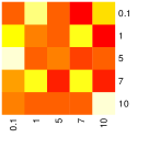
(a) NDCG@1

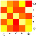
(b) NDCG@3

(c) NDCG@5

Figure 2: $\mu_{1}$ and $\mu_{2}$ heatmap parameter distribution at the different truncation levels $k=1,3,5$ of NDCG@k from the Full Cold Start meta-mining experiments. The figure explanation is as before.

5.4 MovieLens

The MovieLens recommendation dataset has a quite different morphology than that of the meta-mining. The descriptions of the users and the items are much more limited; users are described only by four features: sex, age, occupation and location, and movies by their genre which takes 19 different values, such as comedy, sci-fi to thriller, etc. We model these descriptors using one-of-N representation.

In the MovieLens dataset the side information has been mostly used to regularize the latent profiles and not to predict them, see e.g [1, 2]. Solving the cold start problem in the presence of so limited side information is a rather difficult task and typical collaborative filtering approaches make only use of the preference matrix $\mathbf{Y}$ to learn the user and items latent factors.

5.4.1 Evaluation setting

We use the same baseline methods as in the meta-mining problem. We train LM with the following hyper-parameter setting: we fix the maximum number of nodes for the regression trees to 100, the maximum percentage of instances in each leaf node to $1\%$, and the learning rate, $\eta$, of the gradient boosted tree algorithm to $10^{-2}$. As in the meta-mining problem for the construction of the ensemble of regression trees in LM-MF and LM-MF-Reg we use the same setting for the hyperparameters they share with LM. We optimize their $\mu_{1}$ and $\mu_{2}$ regularization parameters within the grid $[0.1,1,5,$ $10,15,20,25,50,80,100]^{2}$ using five-fold inner cross validation. We fix the number of factors $r$ to 50 and the number of nearest neighbors in the Laplacian matrices to five. As in the meta-mining problem we used the NDCG similarity measure to define output-space similarities with the truncation level $k$ set to the same value as the one at which we evaluate the methods.

We will evaluate and compare the different methods under the two cold start scenarios we described previously. In the user cold start problem, we randomly select 50% of the users for training and we test the recommendations that the learned models generate on the remaining 50%. In the full cold start problem, we use the same separation to training and testing users and in addition we also randomly divide the item set to two equal size subsets, where we use one for training and the other for testing. Thus the learned models are evaluated on users and items that have never been seen in the model training phase. We give the results for the 100k and 1M variants of the MovieLens dataset for the user cold start scenario in table 4a and for the full cold start scenario in table 4b.

5.4.2 Results

In the user cold start scenario, table 4a, we can see first that both LM-MF and LM-MF-Reg beat in a statistically significant manner the UB baseline in both MovieLens variants for all values of the truncation parameter, with the single exception of LM-MF at 100k and $k=5$ for which the performance difference is not statistically significant. LM and its weighted NDCG variant, LMW, are never able to beat UB; LM is even statistically significantly worse compared to UB at 1M for $k=5$. Moreover both LM-MF and its regularized variant beat in a statistically significant manner LM in both MovieLens variants and for all values of $k$. LM-MF-Reg has a small advantage over LM-MF for 100K, it achieves a higher average NDCG score, however this advantage disappears when we move to the 1M dataset, which is rather normal since due to the much larger dataset size there is more need for additional regularization. Moreover since we do a low-rank matrix factorization, we have $r=50$ for the roughly $6000$ users. which already is on its own a quite strong regularization rendering also unnecessary the need for the input/output space regularizers.

A similar picture arises in the full cold start scenario, table 4b. With the exception of MovieLens 100K at $k=10$ both LM-MF and LM-MF-Reg beat always in a statistically significant the FB baseline. Note also that now LM as well as its weigthed NDCG variant are significantly better than the FB baseline for the 1M dataset and $k=5,10$. In adition the weigthed NDCG variant is significantly better than LM for 100k and 1M at $k=5$ and $k=10$ respectively. Both LM-MF and LM-MF-Reg beat in a statistically significant manner LM, with the exception of 100k at $k=10$ where there is no significant difference. Unlike the user cold start problem, now it is LM-MF that achieves the best overall performance.

	$N=5$	$N=10$	$N=15$
CR	0.5755	0.6095	0.7391
LM	0.6093	0.6545	0.7448
$\delta_{CR}$	p=0.4567(=)	p=0.0086(+)	p=1(=)
LMW	0.5909	0.6593	0.7373
$\delta_{CR}$	p=1(=)	p=0.0131(+)	p=0.6985(=)
$\delta_{LM}$	p=0.2626	p=0.0736(=)	p=1(=)
LM-MF	0.6100	0.6556	0.7347
$\delta_{CR}$	p=0.0824(=)	p=0.0255(+)	p=0.6985(=)
$\delta_{LM}$	p=0.7032(=)	p=1(=)	p=0.7750(=)
LM-MF-Reg	0.61723	0.6473	0.7458
$\delta_{CR}$	p=0.0471(+)	p=0.0824(=)	p=0.6985(=)
$\delta_{LM}$	p=0.9005(=)	p=0.8955(=)	p=0.2299(=)

Table 2: NDCG@5 results on meta-mining for the Matrix Completion setting. $N$ is the number of workflows we keep in each dataset for training. For each method, we give the comparison results against the CofiRank and LambdaMart methods in the rows denoted by $\delta_{CR}$ and $\delta_{LM}$ respectively. More precisely we report the $p$-values of the McNemar’s test on the numbers of wins/losses and denote by (+) a statistically significant improvement, by (=) no performance difference and by (-) a significant loss. In bold, the best method for a given $N$.

	k=1	k=3	k=5
UB	0.4367	0.4818	0.5109
LM	0.5219	0.5068	0.5135
$\delta_{UB}$	p=0.0055(+)	p=0.1691(=)	p=0.9005(=)
LMW	0.5008	0.5232	0.5168
$\delta_{UB}$	p=0.0233(+)	p=0.2605(=)	p=0.5319(=)
$\delta_{LM}$	p=0.4291(=)	p=0.1845(=)	p=0.8773(=)
LM-MF	0.5532	0.5612	0.5691
$\delta_{UB}$	p=0.0055(+)	p=0.0086(+)	p=0.3210(=)
$\delta_{LM}$	p=0.0636(=)	p=0.0714(=)	p=0.1271(=)
LM-MF-Reg	0.5577	0.5463	0.5569
$\delta_{UB}$	p=0.0055(+)	p=0.0086(+)	p=0.3815(=)
$\delta_{LM}$	p=0.0636(=)	p=0.1056(=)	p=0.2206(=)

(a) User Cold Start

	$k=1$	$k=3$	$k=5$
FB	0.46013	0.5329	0.5797
LM	0.5192	0.5231	0.5206
$\delta_{FB}$	p=0.0335(+)	p=0.9005(=)	p=0.0607(=)
LMW	0.5294	0.5190	0.5168
$\delta_{FB}$	p=0.0086(+)	p=1(=)	p=0.0175(-)
$\delta_{LM}$	p=1(=)	p=1(=)	p=0.5218(=)
LM-MF	0.5554	0.6156	0.5606
$\delta_{FB}$	p=0.0175(+)	p=0.0175(+)	p=0.6142(=)
$\delta_{LM}$	p=0.0171(+)	p=0.0048(+)	p=0.0211(+)
LM-MF-Reg	0.5936	0.5801	0.5855
$\delta_{FB}$	p=0.0007(+)	p=0.1041(=)	p=1(=)
$\delta_{LM}$	p=0.0117(+)	p=0.0211(+)	p=0.0006(+)

(b) Full Cold Start

Table 3: NDCG@k results on meta-mining for the two cold start settings. For each method, we give the comparison results against the user, respectively full, memory-based and LambdaMart methods in the rows denoted by $\delta_{UB}$, respectively $\delta_{FB}$, and $\delta_{LM}$. The table explanation is as before. In bold, the best method for a given $k$.

	100K		1M
	$k=5$	$k=10$	$k=5$	$k=10$
UB	0.6001	0.6159	0.6330	0.6370
LM	0.6227	0.6241	0.6092	0.6453
$\delta_{UB}$	p=0.2887(=)	p=0.8537(=)	p=0.0001(-)	p=0.1606(=)
LMW	0.6252	0.6241	0.6455	0.6450
$\delta_{UB}$	p=0.0878(=)	p=0.5188(=)	p=0.0120(+)	p=0.1448(=)
$\delta_{LM}$	p=0.7345(=)	p=0.9029(=)	p=0.0000(+)	p=0.5219(=)
LM-MF	0.6439	0.6455	0.6694	0.6700
$\delta_{UB}$	p=0.0036(+)	p=0.1171(=)	p=0.0000(+)	p=0.0000(+)
$\delta_{LM}$	p=$2e^{-06}$(+)	p=$6e^{-06}$(+)	p=0.0000(+)	p=0.0000(+)
LM-MF-Reg	0.6503	0.6581	0.6694	0.6705
$\delta_{UB}$	p=$4e^{-05}$(+)	p=0.0001(+)	p=0.0000(+)	p=0.0000(+)
$\delta_{LM}$	p=$3e^{-06}$(+)	p=0.0000(+)	p=0.0000(+)	p=0.0000(+)

(a) User Cold Start

	100K		1M
	$k=5$	$k=10$	$k=5$	$k=10$
FB	0.5452	0.5723	0.5339	0.5262
LM	0.5486	0.5641	0.5588	0.5597
$\delta_{FB}$	p=0.7817(=)	p=0.4609(=)	p=$1e^{-06}$(+)	p=0.0001(+)
LMW	0.5549	0.5622	0.55737	0.5631
$\delta_{FB}$	p=0.4058(=)	p=0.2129(=)	p=$9e^{-06}$(+)	p=$1e^{-06}$(+)
$\delta_{LM}$	p=0.0087(+)	p=0.8830(=)	p=0.1796(=)	p=$3e^{-06}$(+)
LM-MF	0.5893	0.5876	0.5733	0.5750
$\delta_{FB}$	p=0.0048(+)	p=0.2887(=)	p=0.0000(+)	p=0.0000(+)
$\delta_{LM}$	p=$3e^{-06}$(+)	p=0.0001(+)	p=0.0000(+)	p=0.0000(+)
LM-MF-Reg	0.5699	0.57865	0.5736	0.5683
$\delta_{FB}$	p=0.0142(+)	p=0.1810(=)	p=0.0000(+)	p=$4e^{-07}$(+)
$\delta_{LM}$	p=0.0310(+)	p=0.0722(=)	p=0.0000(+)	p=0.0000(+)

(b) Full Cold Start

Table 4: NDCG@k results on the two MovieLens datasets for the two cold start setting. For each method, we give the comparison results against the user, respectively full, memory-based and LambdaMART methods in the rows denoted by $\delta_{UB}$, respectively $\delta_{FB}$, and $\delta_{LM}$. The table explanation is as before. In bold, the best method for a given $k$.

6 Conclusion

Since only top items are observable by users in real recommendation systems, we believe that ranking loss functions that focus on the correctness of the top item predictions are more appropriate for this kind of problem. We explore the use of a state of the art learning to rank algorithm, LambdaMART, in a recommendation setting with an emphasis on the cold-start problem one of the most challenging problems in recommender systems. However plain vanilla LambdaMART has a certain number of limitations which spring namely from the fact that it lacks a principled way to control overfitting relying in ad-hoc approaches. We proposed a number of ways to deal with these limitations. The most important is that we cast the learning to rank problem as learning a low-rank matrix factorization; our underlying assumption here being that the descriptions of the users and items as well as their preference behavior are governed by a few latent factors. The user item-preferences are now computed as inner products of the learned latent representations of users and items. In addition to the regularization effect of the low rank factorization we bring in additional regularizers to control the complexity of the latent representations, regularizers which reflect the users and items manifolds as these are explicited by user and item feature descriptions as well as the preference behavior. We report results on two very different recommendation problems, meta-mining and MovieLens, and show that the performance of the algorithms we propose beats in a statistically significant manner a number of baselines often used in recommendation systems.

References

- [1] J. Abernethy, F. Bach, T. Evgeniou, and J.-P. Vert. Low-rank matrix factorization with attributes. arXiv preprint cs/0611124, 2006.
- [2] D. Agarwal and B.-C. Chen. flda: matrix factorization through latent dirichlet allocation. In Proceedings of the third ACM international conference on Web search and data mining, WSDM ’10, pages 91–100, New York, NY, USA, 2010. ACM.
- [3] R. M. Bell and Y. Koren. Scalable collaborative filtering with jointly derived neighborhood interpolation weights. In Data Mining, 2007. ICDM 2007. Seventh IEEE International Conference on, pages 43–52. IEEE, 2007.
- [4] C. J. Burges. From ranknet to lambdarank to lambdamart: An overview. Learning, 11:23–581, 2010.
- [5] C. J. Burges, K. M. Svore, P. N. Bennett, A. Pastusiak, and Q. Wu. Learning to rank using an ensemble of lambda-gradient models. Journal of Machine Learning Research-Proceedings Track, 14:25–35, 2011.
- [6] P. Donmez, K. M. Svore, and C. J. Burges. On the local optimality of lambdarank. In Proceedings of the 32nd international ACM SIGIR conference on Research and development in information retrieval, pages 460–467. ACM, 2009.
- [7] J. H. Friedman. Greedy function approximation: a gradient boosting machine. Annals of Statistics, pages 1189–1232, 2001.
- [8] J. Fürnkranz and E. Hüllermeier. Preference learning. Springer, 2010.
- [9] M. Hilario, P. Nguyen, H. Do, A. Woznica, and A. Kalousis. Ontology-based meta-mining of knowledge discovery workflows. In N. Jankowski, W. Duch, and K. Grabczewski, editors, Meta-Learning in Computational Intelligence. Springer, 2011.
- [10] K. Järvelin and J. Kekäläinen. Ir evaluation methods for retrieving highly relevant documents. In Proceedings of the 23rd annual international ACM SIGIR conference on Research and development in information retrieval, pages 41–48. ACM, 2000.
- [11] P. Nguyen, J. Wang, M. Hilario, and A. Kalousis. Learning heterogeneous similarity measures for hybrid-recommendations in meta-mining. In IEEE 12th International Conference on Data Mining (ICDM), pages 1026 –1031, dec. 2012.
- [12] N. Srebro, J. D. M. Rennie, and T. S. Jaakkola. Maximum-margin matrix factorization. In L. K. Saul, Y. Weiss, and L. Bottou, editors, Advances in Neural Information Processing Systems 17, pages 1329–1336. MIT Press, Cambridge, MA, 2005.
- [13] M. Weimer, A. Karatzoglou, Q. V. Le, and A. Smola. Maximum margin matrix factorization for collaborative ranking. Advances in neural information processing systems, 2007.
- [14] Y. Yue and C. Burges. On using simultaneous perturbation stochastic approximation for ir measures, and the empirical optimality of lambdarank. In NIPS Machine Learning for Web Search Workshop, 2007.