Preservation Macroscopic Entanglement of Optomechanical Systems in non-Markovian Environment

Abstract

We investigate dynamics of an optomechanical system under the Non-Markovian environment. In the weak optomechanical single-photon coupling regime, we provide an analytical approach fully taking into account the non-Markovian memory effects. When the cavity-bath coupling strength crosses a certain threshold, an oscillating memory state for the classical cavity field (called bound state) is formed. Due to the existence of the non-decay optical bound state, a nonequilibrium optomechanical thermal entanglement is preserved even without external driving laser. Our results provide a potential usage to generate and protect entanglement via Non-Markovian environment engineering.

Introduction.-The investigation of decoherence and dissipation process induced by environment is a fundamental issue in quantum physics Breuer2002 ; Weiss2008 ; DiVincenzo393 ; Knill409 46 . Understanding the dynamics of such nonequilibrium open quantum system is a challenge topic which provides us the insight into the issue of quantum-classical transitions. Protecting the quantum property from decoherence is a key problem in quantum information science, therefore a lot of effort has been devoted in developing methods for isolating systems from their destructive environment. Recently, people recognize that properly engineering quantum noise can counteract decoherence and can even be used in robust quantum state generation cirac ; Eisert . Meanwhile the features of the non-Markovian quantum process have sparked a great interest in both theoretical and experimental studies Chru104 070406 ; Xu104 100502 ; Liu7 931 ; Chin109 233601 ; Deffner111 010402 . Numerous quantitative measures have been proposed to quantify non-Markovianity Rivas105 050403 ; Breuer103 210401 ; Vasile84 052118 ; Lorenzo88 020102 ; Chru112 120404 .

As a promising candidate for the exploration of quantum mechanical features at mesoscopic and even macroscopic scales and for quantum information procession, cavity optomechanical systems come as a well-developed tool and have received a lot of attentions Vitali98 030405 ; Kippenberg321 1172 ; Groblacher460 724 ; Connell464 697 ; Thompson452 900 . In the theoretical research of the cavity optomechanical system, the environment is often treated as a collective non-interacting harmonic oscillators, and the quantum Langevin equations Giovannetti63 023812 are developed to describe the radiation-pressure dynamic backaction phenomena. Significant progresses have been made in this framework Vitali98 030405 ; Genes77 033804 ; Agarwal81 041803 ; Rabl107 1 . Almost all of these studies are focussing on the scenario of memoryless environment. However in many situations for optical microcavity system, the backaction of the environment and the memory effect of the bath play a significant role in the decoherence dynamics Bayindir84 2140 ; Hartmann2 849 . Quite recently, a nonorthodox decoherence phenomenon of the mechanical resonator is also observed in experiment Groblacher6 7606 , which clearly reveals the non-Markovian nature of the dynamics. Therefore, it is the time to investigate the non-Markovian environment engineering for the nonlinear cavity optomechanical system so that we can use the memory effects to produce and protect coherence within it.

In this Letter, we investigate the cavity optomechanical dynamics under Non-Markovian environment and put forward a method to solve the exact Heisenberg-Langevin equations where the non-local time-correlation of the environment is included. We find that when the cavity-bath coupling strength crosses a certain threshold, the optical bound state is formed, giving rise to the nonequilibrium dynamics of the entanglement. This remarkable result indicates the possibility of long-time protection of macroscopic entanglement via structured reservoirs.

Model.-We consider a generic cavity optomechanical system consisting of a Fabry-Pérot cavity with a movable mirror at one side. The cavity has equilibrium length $L$, while the movable mirror has effective mass $m$. As shown in Fig. 1, cavity environment could be a coupled-resonator optical waveguide which possesses strong non-Markovian effects Wu18 18407 , and the micro-mechanical resonator and its environment could be the device of a high-reflectivity Bragg mirror fixed in the centre of a doubly clamped $\mathrm{Si_{3}N_{4}}$ beam in vacuum Groblacher6 7606 . The corresponding Hamiltonian of the system can be written as Giovannetti63 023812 ; Genes77 033804 $\hat{H}_{S}=\hbar\omega_{c}\hat{a}^{{\dagger}}\hat{a}+\frac{\hbar\omega_{m}}{2}(\hat{p}^{2}+\hat{q}^{2})-\hbar g_{0}\hat{a}^{{\dagger}}\hat{a}\hat{q}+i\hbar E(e^{-i\omega_{0}t}\hat{a}^{{\dagger}}-e^{i\omega_{0}t}\hat{a}).$ Here $\omega_{c}$ is the frequency of the cavity mode with bosonic operators $\hat{a}$ and $\hat{a}^{{\dagger}}$ satisfying $[\hat{a},\hat{a}^{{\dagger}}]=1$, while the quadratures $\hat{q}$ and $\hat{p}$ ($[\hat{q},\hat{p}]=i$) are associated to the mechanical mode with frequency $\omega_{m}$. The third term describes the optomechanical interaction at the single-photon level with coupling coefficient $g_{0}=(\omega_{c}/L)\sqrt{\hbar/2m\omega_{m}}$. The cavity is driven by an external laser with the center frequency $\omega_{0}$. The environment of such system can be described by a collection of independent harmonic oscillators Ford37 4419 . The reservoir as well as the system-reservoir interaction is then given by $\hat{H}_{EI}=\sum_{k}{\hbar(\omega_{k}\hat{a}_{k}^{{\dagger}}\hat{a}_{k}}+\hbar g_{k}\hat{a}^{{\dagger}}\hat{a}_{k}+\hbar g_{k}^{\ast}\hat{a}_{k}^{{\dagger}}\hat{a})+\sum_{l}\frac{\hbar\omega_{l}}{2}[\hat{q}_{l}^{2}+(\hat{p}_{l}-\gamma_{l}\hat{q})^{2}].$ The first term is the free energy of the cavity reservoir with the continuous frequency $\omega_{k}$ as well as the hopping interaction between the cavity and the environment with the coupling strength $g_{k}$. The second summation describes a mirror undergoing Brownian motion with the coupling through the reservoir momentum Giovannetti63 023812 ; Ford37 4419 . Here $\omega_{l}$ is the reservoir energy of the mechanical mode, and $\gamma_{l}$ stands for the mirror-reservoir coupling.

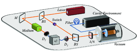
Figure 1: (Color online) Example implementations of optomechanical system setup for study the non-Markovian dynamics: a laser is split into a signal beam and a local oscillator. The signal (input field) is controlled by the Switch and the output field can be read through photon detectors. The optomechanical cavity environment is introduced by a low-loss fiber. The optomechanical cavity is kept at a pressure of $<10^{-3}$ mbar to avoid residual-gas damping of the mechanical motion.

Dynamics of the system.-To achieve a comprehensive understanding of the decoherence dynamics, one has to rely on precise model calculations. To this end, by making use of the reference frame rotating at the laser frequency and tracing out all the environmental degrees of freedom, we can obtain the Heisenberg-Langevin equations (see Sec. I in the Supplemental Material)

$$\dot{\hat{a}} = -i\Delta_{c}\hat{a}+ig_{0}\hat{a}\hat{q}-\int_{0}^{t}d\tau f_{c}(t-\tau)\hat{a}(\tau)$$ (1a)

$$-i\sum\limits_{k}g_{k}e^{-i\Delta_{k}t}\hat{a}_{k}(0)+E,$$

$$\dot{\hat{q}} = \omega_{m}\hat{p},$$ (1b)

$$\dot{\hat{p}} = -\Delta_{m}\hat{q}+g_{0}\hat{a}^{{\dagger}}\hat{a}+\int_{0}^{t}d\tau f_{m}(t-\tau)\hat{q}(\tau)$$ (1c)

$$+\sum\limits_{l}\omega_{l}\gamma_{l}(\hat{p}_{l}(0)\cos\omega_{l}t-\hat{q}_{l}(0)\sin\omega_{l}t),$$

where $$\Delta_{c}=\omega_{c}-\omega_{0} \Delta_{k}=\omega_{k}-\omega_{0} k \Delta_{m}=\omega_{m}+\sum_{l}\omega_{l}\gamma_{l}^{2} f_{c}(t)=\sum_{k}g_{k}^{\ast}g_{k}e^{-i\Delta_{k}t} f_{m}(t)=\sum_{l}\omega_{l}^{2}\gamma_{l}^{2}\sin\omega_{l}t J(\omega) f_{c}(t)=\int\frac{d\omega}{2\pi}J_{c}(\omega)e^{-i(\omega-\omega_{0})t} f_{m}(t)=\int\frac{d\omega}{2\pi}J_{m}(\omega)\sin\omega t \hat{q}_{l}(0) \hat{p}_{l}(0) \hat{a}_{k}(0)$$ is the cavity detuning, is the detuning of the -th mode of the environment, and is the reservoir-induced potential energy shift. The non-Markovian effect is fully manifested in Eqs.(1), where the non-local time correlation functions of the environments, i.e., and , are included. By introducing the spectral density of the reservoirs, one can rewrite the time correlation functions as and . The terms containing reservoir operators , and are usually regarded as the noise-input of the system, which depend on the initial states of the reservoirs.

The integro-differential Heisenberg-Langevin equations Eqs.(1) are intrinsically nonlinear. Up to now, most experimental realizations of cavity optomechanics are still in the single-photon weak coupling limit Chan478 89 ; Teufel475 359 ; Arcizet444 71 ; Groblacher460 724 , i.e., $10^{-5}\lesssim g_{0}/\omega_{m}\lesssim 10^{-3}$. When the intracavity photon number $|\langle\hat{a}\rangle|\gg 1$, we can apply the so-called linearization method Genes77 033804 ; Aspelmeyer86 1391 . This means the relevant quantum operators can be expanded about their respective mean values: $\hat{O}=\langle\hat{O}\rangle+\delta\hat{O}$, where $\hat{O}\equiv(\hat{a},\hat{a}^{\dagger},\hat{q},\hat{p})^{T}$, and the superscript $T$ represents the transpose operation. Then Eqs.(1) can be decomposed into two parts. The first is the classical part that describing the classical phase space orbits of the first moments of operators

$$\dot{\alpha} = -i\Delta_{c}\alpha+ig_{0}\alpha q-\int_{0}^{t}d\tau f_{c}(t-\tau)\alpha(\tau)+E,~{}$$ (2)

$$\ddot{q} = -\omega_{m}\Delta_{m}q+g_{0}\omega_{m}|\alpha|^{2}+\omega_{m}\int_{0}^{t}d\tau f_{m}(t-\tau)q(\tau),$$

where, for simplicity, we have assumed $\langle\hat{q}_{l}(0)\rangle=\langle$ $\hat{p}_{l}(0)\rangle$ $=\langle\hat{a}_{k}(0)\rangle=0$. In the single-photon weakly coupling regime, the coupling strength $g_{0}$ is the smallest parameter in Eqs.(2). We therefore perform the regular perturbation expansion in ascending powers of the rescaled dimensionless variable $g_{0}/\omega_{m}$ (for computational convenience one may set $\omega_{m}=1$, and the other rescaled parameters are in units of $\omega_{m}$). By substituting the expressions with rescaled $g_{0}$ (i.e., $\alpha=\sum_{n=0}^{\infty}g_{0}^{n}\alpha_{n}$ and $q=\sum_{n=0}^{\infty}g_{0}^{n}q_{n}$) into the averaged Langevin equations (2), one can give a formal solution up to the first order for the classical part in the framework of modified Laplace transformation Zhang109 170402

$$\alpha_{0}(t) = \alpha(0)\bar{\alpha}_{0}(t)+E\int_{0}^{t}d\tau\bar{\alpha}_{0}(\tau),$$ (3a)

$$q_{0}(t) = \int_{-\infty}^{\infty}\frac{d\omega}{2\pi}\frac{[i\omega q(0)-p(0)]e^{-i\omega t}}{\omega^{2}-\Delta_{m}-K_{m}(\omega)-i\tilde{J}(\omega)},~{}~{}~{}~{}~{}$$ (3b)

$$\alpha_{1}(t) = i\int_{0}^{t}d\tau\bar{\alpha}_{0}(t-\tau)\alpha_{0}(\tau)q_{0}(\tau),$$ (3c)

$$q_{1}(t) = \int_{0}^{t}d\tau\bar{q}_{0}(t-\tau)|\alpha_{0}(\tau)|^{2}$$ (3d)

where $$K_{m}(\omega)=\mathcal{P}\int\frac{d\omega^{\prime}}{2\pi}\frac{\omega^{\prime}J_{m}(\omega^{\prime})}{\omega^{2}-\omega^{\prime 2}} \tilde{J}(\omega)=\frac{J_{m}(-\omega)-J_{m}(\omega)}{4} \bar{\alpha}_{0} \bar{q}_{0} \bar{\alpha}_{0}(0)=1 \bar{q}_{0}(0)=0 \dot{\bar{q}}_{0}(0)=1 \alpha_{0}(\infty) q_{1}(\infty) \tilde{\Delta}=\Delta_{c}-g_{0}^{2}q_{1}(\infty) \tilde{\Delta}\approx\Delta_{c}$$ and are the real and imaginary part of the Laplace transform of the self-energy correction respectively, and the Green’s functions and obey the Dyson equations (S6) and (S7) with the initial conditions , and Zhang109 170402 . Base on Eqs. (3), we can see that the non-vanishing intracavity field may induce an equilibrium position for the oscillator. This leads to the effective cavity detuning , which also alters the asymptotic dynamics of the cavity field. Accordingly, the interplay between the non-Markovian and nonlinear effects can be described more precisely in this way. Within the parameter space of our consideration, , the validity of the power series assumption is guaranteed by the numerical simulations (see Sec. II in the Supplemental Material).

For general bosonic environments, the spectral density should be a Poisson-type distribution function Leggett59 1 . We consider that the spectrum is of the form

$$J_{a}(\omega)=2\pi\eta_{a}\omega(\frac{\omega}{\tilde{\omega}_{a}})^{s_{a}-1}e^{-\frac{\omega}{\tilde{\omega}_{a}}}~{}~{}~{}~{}(a=c,m),$$

where $\eta_{a}$ is a dimensionless coupling constant between the system and the environment, and $\tilde{\omega}_{a}$ is a high-frequency cutoff Leggett59 1 ; Weiss2008 . The parameter $s_{a}$ classifies the environment as sub-Ohmic $(0<s_{a}<1)$, Ohmic $(s_{a}=1)$, and super-Ohmic $(s_{a}>1)$. Using the modified Laplace transformation, one can give an analytical solution for the nonequilibrium Green’s function

$$\bar{\alpha}_{0}(t) = \mathcal{Z}e^{-i\omega_{r}t}$$

$$+\frac{2}{\pi}\int_{-\omega_{0}}^{\infty}d\omega\frac{J_{c}(\omega+\omega_{0})e^{-i\omega t}}{4[\omega-\Delta_{c}-K_{c}(\omega)]^{2}+J_{c}^{2}(\omega+\omega_{0})}$$

with $K_{c}(\omega)=\mathcal{P}\int\frac{d\omega^{\prime}}{2\pi}\frac{J_{c}(\omega^{\prime})}{\omega-\omega^{\prime}+\omega_{0}}$. The first term survives only when $\omega_{c}+K_{c}(-\omega_{0})\leq 0$, the residue $\mathcal{Z}=[1-K_{c}^{\prime}(\omega)]^{-1}$, and the pole $\omega_{r}$ is located at the real $z$ axis. This term  corresponds to “localized mode” Zhang109 170402 ; Cheng91 022328 , which means that the cavity field oscillates with frequency $\omega_{r}$ and does not decay. It is seem that the photons are “trapped” in the cavity due to the backflow of the non-Markovian environment and do not diffuse. It is a term that determines the asymptotic dynamics of the optical field. Physically, this is equivalent Cheng91 022328 to generate a bound state of the joint cavity-reservoir system, which can be also determined Tong81 052330 by solving the energy eigenstates of the total Hamiltonian, and such bound state is actually a stationary state with a vanishing decay rate during the time evolution. The second term corresponds to nonexponential decays. In the long time limit, the bound state as well as the driving laser give rise to the non-vanishing intracavity photon numbers with $\alpha_{0}(\infty)=\frac{\omega_{r}\alpha(0)+iE}{\omega_{r}[1-K_{c}^{\prime}(\omega_{r})]}e^{-i\omega_{r}t}-\frac{iE}{\Delta_{c}+K_{c}(0)-\frac{i}{2}J_{c}(\omega_{0})}$. On the other hand, for the mechanical mode, however, due to the discontinuity of the self-energy correction at the real $z$ axis, $q_{0}(\infty)=0$. We find that the corresponding mechanical bound state can be formed only if some sharp cutoff appear in the spectral density (see Supplemental Material Sec. II).

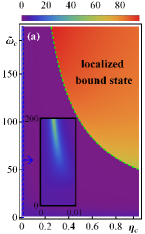
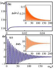
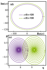
Figure 2: (Color online) Classical dynamics in an optomechanical system, in units of $\omega_{m}$. (a) is the density plot of $|\alpha_{0}|_{max}(\infty)$, in which we show the region in the parameter space of coupling $\eta_{c}$ and frequency cutoff $\tilde{\omega}_{c}$, where significant bound state exist with $E=10\omega_{m}$ and $\Delta_{c}=2\omega_{m}$. Plot (b-e) show the dynamical evolution of the classical variables, where $g_{0}=6\times 10^{-4}\omega_{m}$, $\ \eta_{m}=0.03$, $\tilde{\omega}_{m}=11\omega_{m}$ and $E=0$. The other parameters are $\eta_{c}=0.05$, $s_{c}=3$, $s_{m}=1$, $\tilde{\omega}_{c}=11\omega_{c}=1100\omega_{m}$, $\alpha(0)=120$, $p(0)=0$, and we keep $q(0)=\frac{g_{0}}{\omega_{m}}|\alpha(0)|^{2}$.

Considering the feasibility, the single photon coupling $g_{0}$ (key parameter) is set close to that of recently performed optomechanical experiments Aspelmeyer86 1391 . Fig. 2(a) is the density plot of the maximum value of $|\alpha_{0}|$ in the long-time limit. It maps out the regions in parameter space where localized bound state occurs. As a result, a threshold characterizing the transition from weak to strong non-Markovian regions can be defined, and it is marked by the green-dashed line, which satisfying $\omega_{c}+K_{c}(-\omega_{0})=0$. In the weakly non-Markovian region $0<\eta_{c}<0.01$, as shown in the inset of Fig. 2(a), the red-detuned laser gives rise to a strong stationary amplitude values, which is determined by $\frac{iE}{\frac{i}{2}J_{c}(\omega_{0})-\Delta_{c}-K_{c}(0)}$. Figs. 2(b) and 2(c) show the dynamic evolution of $|\alpha_{0}|$ and $q_{0}$, where the first order solutions are shown in the insets. In Fig. 2(b) the optical bound state is formed when $\eta_{c}$ is above the threshold, while for Fig. 2(c), the coordinate average value of the oscillator is no longer zero, which reveals that radiation pressure push the oscillator to a new equilibrium position. The evolution in the phase space is shown in Figs. 2(d) and 2(e). The limit cycles that characterize the properties of the steady state depends on the initial states, which indicates the non-Markovian property and reflects the memory effect. The initial information of the system is maintained.

We now turn to the quantum fluctuation of operators that describes the actual quantum dynamics, which are deduced as

$$\delta\dot{\hat{O}}=M(t)\delta\hat{O}-\int_{0}^{t}d\tau F(t-\tau)\delta\hat{O}(\tau)+\hat{\xi}(t).$$ (5)

By assuming the formal solution $\delta\hat{O}=\mathcal{U}(t)\delta\hat{O}(0)+\hat{\mathcal{V}}(t)$, and substituting it into Eq. (5), we have

$$\dot{\mathcal{U}}(t) = M(t)\mathcal{U}(t)-\int_{0}^{t}d\tau F(t-\tau)\mathcal{U}(\tau),$$ (6a)

$$\dot{\hat{\mathcal{V}}}(t) = M(t)\hat{\mathcal{V}}(t)-\int_{0}^{t}d\tau F(t-\tau)\hat{\mathcal{V}}(\tau)+\hat{\xi}(t),~{}~{}~{}$$ (6b)

subjected to the initial conditions $$\mathcal{U}(0)=\mathbf{I} \hat{\mathcal{V}}(0)=0 4\times 4$$ and . The matrix

$$M(t)=\left(\begin{array}[]{cccc}-i\Delta_{cq}(t)&0&ig_{0}\alpha(t)&0\\ 0&i\Delta_{cq}(t)&-ig_{0}\alpha^{\ast}(t)&0\\ 0&0&0&\omega_{m}\\ g_{0}\alpha^{\ast}(t)&g_{0}\alpha(t)&-\Delta_{m}&0\end{array}\right)$$

describes the linearized optomechanical coupling with non-local time-dependent classical variables, where $\Delta_{cq}(t)=\Delta_{c}-g_{0}q(t)$ and $\Delta_{m}=\omega_{m}+\eta_{m}\tilde{\omega}_{m}\Gamma(s_{m})$. The matrix

$$F(t)=\left(\begin{array}[]{cccc}f_{c}(t)&0&0&0\\ 0&f_{c}^{\ast}(t)&0&0\\ 0&0&0&0\\ 0&0&-f_{m}(t)&0\end{array}\right)$$

depicts the time correlation of the optomechanical system in the bosonic environments. The last term $\hat{\xi}(t)=(-i\sum_{k}g_{k}e^{-i\Delta_{k}t}\hat{a}_{k}(0),i\sum_{k}g_{k}^{\ast}e^{i\Delta_{k}t}\hat{a}_{k}^{{\dagger}}(0),0,\sum_{l}\omega_{l}\gamma_{l}[\hat{p}_{l}(0)\newline \times\cos\omega_{l}t-\hat{q}_{l}(0)\sin\omega_{l}t])^{T}$ is interpreted as a noise term Giovannetti63 023812 ; Genes77 033804 that depends on the initial states of the environments. It is easy to obtain the quadrature operator $\hat{R}\equiv(\delta\hat{x}_{c},\delta\hat{p}_{c},\delta\hat{q},\delta\hat{p})^{T}$ through the relation $\hat{R}=\mathcal{S}\delta\hat{O}$, where $\mathcal{S}$ is the transformation matrix. Then the covariance matrix with components $V_{ij}=\langle\hat{R}_{i}\hat{R}_{j}+\hat{R}_{j}\hat{R}_{i}\rangle/2$ can be determined by calculating the time evolution of the second moments of the quadratures

$$\hat{R}\hat{R}^{T} = \mathcal{S}\mathcal{U}\mathcal{S}^{-1}\hat{R}(0)\hat{R}^{T}(0){\mathcal{S}^{-1}}^{T}\mathcal{U}^{T}\mathcal{S}^{T}+\mathcal{S}\hat{\mathcal{V}}\hat{\mathcal{V}}^{T}\mathcal{S}^{T}$$

$$+\mathcal{S}\mathcal{U}\mathcal{S}^{-1}\hat{R}(0)\hat{\mathcal{V}}^{T}\mathcal{S}^{T}+\mathcal{S}\hat{\mathcal{V}}\hat{R}^{T}(0){\mathcal{S}^{-1}}^{T}\mathcal{U}^{T}\mathcal{S}^{T}.~{}~{}~{}$$

The first term is the projection of the quadratures on the system’s Hilbert space. The second term characterizes the magnitudes of the input-noise that satisfies the non-local time correlation relations Giovannetti63 023812 . The last two terms describe the effect of initial system-reservoir correlations, which had been identified as an important factor in the decoherence dynamics Romero55 4070 ; Dijkstra104 250401 . For the sake of simplicity, here we assume as usual the system and the reservoirs are initially uncorrelated, and the reservoirs are in thermal states. Then the noise vector $\hat{\xi}(t)$ obeys the non-Markovian self-correlation $\langle\hat{\xi}(t)\hat{\xi}(t^{\prime})\rangle=G_{c}(t-t^{\prime})\oplus G_{m}(t-t^{\prime})$, where $G_{c}$ and $G_{m}$ are $2\times 2$ matrix

$$G_{c}(\tau)=\left(\begin{array}[]{cc}0&\tilde{g}_{c}(\tau)\\ g_{c}(-\tau)&0\end{array}\right),~{}~{}~{}G_{m}(\tau)=\left(\begin{array}[]{cc}0&0\\ 0&g_{m}(\tau)\end{array}\right).$$

The thermal correlation functions are defined as $g_{c}(\tau)=\int\frac{d\omega}{2\pi}J_{c}(\omega)\frac{e^{-i(\omega-\omega_{0})\tau}}{e^{\beta_{c}\omega}-1}$, $\tilde{g}_{c}(\tau)=\int\frac{d\omega}{2\pi}J_{c}(\omega)\frac{e^{\beta_{c}\omega-i(\omega-\omega_{0})\tau}}{e^{\beta_{c}\omega}-1}$ and $g_{m}(\tau)=\int\frac{d\omega}{4\pi}J_{m}(\omega)(\frac{2\cos{\omega\tau}}{e^{\beta_{m}\omega}-1}+e^{-i\omega\tau})$, where $\beta=1/k_{B}T$, $k_{B}$ is the Boltzmann constant and $T$ is the initial temperature of the reservoir.

Preservation of entanglement To bring quantum effects to the macroscopic level, one important way is the creation of entanglement between the optical mode and the mechanical mode. If the initial states of the system is Gaussian, then Eq. (5) will preserve the Gaussian character. The entanglement can therefore be quantified via the logarithmic negativity Adesso72 032334 defined as $E_{\mathcal{N}}=\max[0,-\ln(2s^{-})]$, where $s^{-}$ is the smallest symplectic eigenvalues of the partially transposed covariance matrix $V^{T_{A}}$.

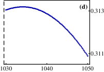
Figure 3: (Color online) Time evolution of pseudoentanglement $E_{p}$ in Ohmic environment. In (a) and (b), we keep $s_{m}=1$, while in (c) and (d), $s_{m}=3$, $\eta_{m}=0.8$ and $\tilde{\omega}_{m}=5\omega_{m}$. The other parameters are the same as Fig. 2(b). The dynamical evolution of entanglement are shown in three regions, the initial stage of evolution $\omega_{m}t<5\times 10^{-3}$ shown in the insets of (a) and (c) , the short-time scale $\omega_{m}t<50$ corresponding to (a) and (c), the long-time scale $\omega_{m}t$ around $1040$ for (b) and (d). The regions $E_{p}<0$ correspond to nonphysical results.

$\omega_{m}t$

The non-Markovian effect generally lead to the nonequilibrium dynamics, therefore, we explore the optomechanical entanglement in transient regime. In order to show clearly the evolutionary path of the entanglement, we use the so-called pseudoentanglement measure Wang112 110406 defined as $E_{p}=-\ln(2s^{-})$, so that the logarithmic negativity of entanglement measure $E_{\mathcal{N}}=\max[0,E_{p}]$. For simplicity, we assume the bath of the cavity initially in vacuum and the cavity initially in coherent state with $\alpha(0)=120$. The results are plotted in Fig. 3, in which $\beta_{m}=2.5\times 10^{-2}\omega_{m}^{-1}$ (the corresponding thermal excitation number are $n_{m}\approx 40$). In order to show clearly the phenomenon of entanglement preservation by non-Markovianity, we shutoff the classical pumping field all the time by setting $E=0$. We see in Fig. 3 that the shape of the Ohmic spectrum characterized by $s_{m}$, has effect on the entanglement dynamics in the short-time and long-time scale, but has negligible impact on the initial stage of evolution (see the insets). This is because the time scale of the mechanical oscillator as well as its bath is much larger than that of the bath of the cavity, which means the non-Markovian memory effects induced by the bath of the oscillator can be ignored completely when $t\ll 1/d$, where $d$ is the bandwidth of the oscillator’s bath. Although the sudden death and rebirth of entanglement is also observed, it differ with the case of Markovian environment Yu323 598 where the photons would rapidly dissipate to the memoryless environment. Here, due to the present of the bound state, the entanglement can be produced and can be preserved in non-Markovian environment after long time even without external drive. This provides a way to decoherence control of optomechanical systems, in which, a controllable quantum environment indeed have the ability to protect the quantum correlation of the internal system.

Conclusion We have put forward a scheme to preserve the entanglement of optomechanical system in non-Markovian environment. An analytical approach for describing non-Markovian memory effects that impact on the decoherence dynamics of an optomechanical system is presented. The exact Heisenberg-Langevin equations are derived, and the perturbation solution is given in the weak single-photon coupling regime. Employing the analytical solution, we have shown that, the system dynamics change dramatically when the cavity-bath coupling strength crosses a certain threshold, which corresponds to dissipationless non-Markovian dynamics. The interplay between non-Markovian and nonlinear effects can be also explained though the perturbative method. As a quantum device which may subjected to dissipative and decoherence effects, however, our results show that the surroundings of such a simple setting can protect the quantum entanglement, rather than destroy it even in the long-time scales, which means that engineered quantum noise can be used in robust quantum state generation. Our research provides a new approach to explore non-Markovian dynamics for the cavity optomechanical systems.

Acknowledgment We would like to thank B.-L. Hu, P.-Y. Lo, H.-N. Xiong and W.-L. Li for helpful discussions. This work is supported by the NSF of China under Grant No. 11474044.

References

- (1) H.-P. Breuer and F. Petruccione, The Theory of Open Quantum Systems (Oxford University Press, Oxford, UK, 2002).
- (2) U. Weiss, Quantum Dissipative Systems, 3rd ed. (World Scientific Press, Singapore, 2008).
- (3) D. P. DiVincenzo, Nature 393, 113 (1998).
- (4) E. Knill, R. Laflamme, and G. J. Milburn, Nature 409, 46 (2001).
- (5) F. Verstraete, M. M. Wolf, and J. I. Cirac, Nature Phys. 5, 633 (2009).
- (6) M. J. Kastoryano, M. M. Wolf, and J. Eisert, Phys. Rev. Lett. 110, 110501 (2013).
- (7) D. Chruściński and A. Kossakowski, Phys. Rev. Lett. 104, 070406 (2010).
- (8) J.-S. Xu, et al., Phys. Rev. Lett. 104, 100502 (2010).
- (9) B.-H. Liu, et al., Nat. Phys. 7, 931 (2011).
- (10) A. W. Chin, S. F. Huelga, and M. B. Plenio, Phys. Rev. Lett. 109, 233601 (2012).
- (11) S. Deffner and E. Lutz, Phys. Rev. Lett. 111, 010402 (2013).
- (12) Á. Rivas, S. F. Huelga, and M. B. Plenio, Phys. Rev. Lett. 105, 050403 (2010).
- (13) H.-P. Breuer, E.-M. Laine, and J. Piilo, Phys. Rev. Lett. 103, 210401 (2009).
- (14) R. Vasile, S. Maniscalco, M. G. A. Paris, H.-P. Breuer, and J. Piilo, Phys. Rev. A 84, 052118 (2011).
- (15) S. Lorenzo, F. Plastina, and M. Paternostro, Phys. Rev. A 88, 020102 (2013).
- (16) D. Chruściński and S. Maniscalco, Phys. Rev. Lett. 112, 120404 (2014).
- (17) D. Vitali et al., Phys. Rev. Lett. 98, 030405 (2007).
- (18) T. J. Kippenberg and K. J. Vahala, Science 321, 1172 (2008).
- (19) S. Gröblacher, K. Hammerer, M. R. Vanner, and M. Aspelmeyer, Nature (London) 460, 724 (2009).
- (20) A. D. O’Connell et al., Nature (London) 464, 697 (2010).
- (21) J. D. Thompson et al., Nature 452, 900 (2008).
- (22) V. Giovannetti and D. Vitali, Phys. Rev. A 63, 023812 (2001).
- (23) C. Genes, D. Vitali, P. Tombesi, S. Gigan, and M. Aspelmeyer, Phys. Rev. A 77, 033804 (2008).
- (24) G. S. Agarwal and S. Huang, Phys. Rev. A 81, 041803 (2010).
- (25) P. Rabl, Phys. Rev. Lett. 107, 063601 (2011).
- (26) M. Bayindir, B. Temelkuran, and E. Ozbay, Phys. Rev. Lett. 84, 2140 (2000).
- (27) M. J. Hartmann, F. G. S. Brandao, and M. Plenio, Nature Phys. 2, 849 (2006).
- (28) S. Gröblacher, A. Trubarov, N. Prigge, G. D. Cole, M. Aspelmeyer and J. Eisert, Nature Commun. 6, 7606 (2015).
- (29) M. H. Wu, C. U. Lei, W. M. Zhang, and H. N. Xiong, Opt. Express 18, 18407 (2010).
- (30) G. W. Ford, J. T. Lewis, and R. F. O’Connell, Phys. Rev. A 37, 4419 (1988).
- (31) J. Chan, T. P. M. Alegre, A. H. Safavi-Naeini, J. T. Hill, A. Krause, S. Gröblacher, M. Aspelmeyer, and O. Painter, Nature (London) 478, 89 (2011).
- (32) J. D. Teufel et al. Nature (London) 475, 359 (2011).
- (33) O. Arcizet, P.-F. Cohadon, T. Briant, M. Pinard, and A. Heidmann, Nature (London) 444, 71 (2006).
- (34) M. Aspelmeyer, T. J. Kippenberg, and F. Marquardt, Rev. Mod. Phys. 86, 1391 (2014).
- (35) W. M. Zhang, P. Y. Lo, H. N. Xiong, Matisse Wei-Yuan Tu , and F. Nori, Phys. Rev. Lett. 109, 170402 (2012).
- (36) A. J. Leggett, S. Chakravarty, A. T. Dorsey, M. P. A. Fisher, A. Garg and W. Zwerger, Rev. Mod. Phys. 59, 1 (1987).
- (37) J. Cheng, W.-Z. Zhang, Y. Han, and L. Zhou, Phys. Rev. A 91, 022328 (2015).
- (38) Q. J. Tong, J. H. An, H. G. Luo, and C. H. Oh, Phys. Rev. A 81, 052330 (2010).
- (39) L. D. Romero and J. P. Paz, Phys. Rev. A 55, 4070 (1997).
- (40) A. G. Dijkstra and Y. Tanimura, Phys. Rev. Lett. 104, 250401 (2010).
- (41) G. Adesso and F. Illuminati Phys. Rev. A 72, 032334 (2005).
- (42) G. Wang, L. Huang, Y.-C. Lai, and C. Grebogi, Phys. Rev. Lett. 112, 110406 (2014).
- (43) T. Yu and J. H. Eberly, Science 323, 598 (2009).