The WR-HSS iteration method for a system of linear
differential equations and its applications to
the unsteady discrete elliptic problem

Abstract

We consider the numerical method for non-self-adjoint positive definite linear differential equations, and its application to the unsteady discrete elliptic problem, which is derived from spatial discretization of the unsteady elliptic problem with Dirichlet boundary condition. Based on the idea of the alternating direction implicit (ADI) iteration technique and the Hermitian/skew-Hermitian splitting (HSS), we establish a waveform relaxation (WR) iteration method for solving the non-self-adjoint positive definite linear differential equations, called the WR-HSS method. We analyze the convergence property of the WR-HSS method, and prove that the WR-HSS method is unconditionally convergent to the solution of the system of linear differential equations. In addition, we derive the upper bound of the contraction factor of the WR-HSS method in each iteration which is only dependent on the Hermitian part of the corresponding non-self-adjoint positive definite linear differential operator. Finally, the applications of the WR-HSS method to the unsteady discrete elliptic problem demonstrate its effectiveness and the correctness of the theoretical results.

Keywords: GMRES; HS splitting; SOR; system of linear equations; unsteady discrete elliptic problem; waveform relaxation.

1 Introduction

We consider the numerical solution of the following unsteady elliptic problem (second-order parabolic equation),

$$\left\{\begin{array}[]{l}\frac{\partial u(x,t)}{\partial t}-\nabla\cdot[a(x,t)\nabla u(x,t)]+\sum_{j=1}^{d}\frac{\partial}{\partial x_{j}}(p(x,t)u(x,t))=q(x,t),\,x\in\Omega,\,t\in[0,\mbox{T}],\\ u(x,0)=u_{0}(x),\,x\in\Omega,\\ u(x,t)=v(x,t),\,x\in\partial\Omega,\,t\in[0,\mbox{T}]\end{array}\right.$$ (1.4)

with $\Omega$ being a plurirectangle of $\makebox{{\mbox{\bb R}}}^{d}$, $\partial\Omega$ being the boundary of the domain $\Omega$, T (possibly infinite) being the upper bound of the time interval, $a(x,t)$ being a uniformly positive function and $p(x,t)$ denoting the Reynolds function. Specifically, plurirectangle here means a connected union of rectangles in $d$-dimensions with edges parallel to the axes. The above equation is important for various reasons [19]. As well as describing many significant physical processes like the transport and diffusion of pollutants, representing the temperature of a fluid moving along a heated wall, or the concentration of electrons in models of semiconductor devices, it is also a fundamental subproblem for models of incompressible flow.

The unsteady elliptic problem can be handled in two different ways such as “Rothe Method” and “Method of Lines”. For the “Rothe Method”, the time variable is discretized firstly by certain time differencing scheme to obtain a sequence of steady problems, and each of these problems is then solved by some spatial discretization method. For the “Method of Lines”, the spatial variable is discretized firstly to obtain a system of ordinary-differential equations (ODEs) or differential-algebraic equations (DAEs), and certain time differencing scheme is then applied to solve the above differential equations.

The waveform relaxation (WR) methods are powerful solvers for numerically computing the solution of ODEs or DAEs on sequential and parallel computers, which was first introduced by Lelarasmee in [24] for simulating the behavior of very large-scale electrical networks. Later, there are lots of expansions and applications of his theory; see, e.g., [15, 23, 25]. The basic idea of this class of iteration methods is to apply relaxation technique directly to the corresponding differential equations, which can be regarded as a natural extension of the classical relaxation methods for solving systems of linear equations with iterating space changing from $\makebox{{\mbox{\bb R}}}^{n}$ to the time-dependent function or the waveform space.

In order to take advantage of the waveform relaxation methods for solving the unsteady elliptic problem (1.4), we follow the first step of “Method of Lines” to discretize (1.4) spatially with spatial grid parameter $h$ to obtain the so-called unsteady discrete elliptic problem as follows,

$$\mathcal{L}_{h}(x)=B\,\dot{x}(t)+A\,x(t)=f(t),\quad x(0)=x_{0},$$ (1.5)

with $B\in\makebox{{\mbox{\bb C}}}^{r\times r}$ being Hermitian and $A\in\makebox{{\mbox{\bb C}}}^{r\times r}$ being non-Hermitian positive definite, the solution $x(t)$ and the data $f(t)$ are complex vector-valued functions. It can be proved that the linear differential operator $\mathcal{L}_{h}$ is non-self-adjoint positive definite on Lebesgue square-integrable function space under suitable conditions. Therefore, this operator $\mathcal{L}_{h}$ can be considered as the analogous of non-Hermitian positive definite matrix. For systems of linear equations related to non-Hermitian positive definite coefficient matrix, Bai, Golub and Ng [9] proposed a class of two-step iterative methods, called the HSS method, which is designed in the spirit of the ADI iteration technique [16] and by making use of the natural splitting of non-Hermitian positive definite matrix, i.e., the HS splitting. Similar to the HS splitting of matrix, we define the HS splitting of the non-self-adjoint positive definite linear differential operator $\mathcal{L}_{h}$, and design the waveform relaxation method based on the HS spitting of operator $\mathcal{L}_{h}$, i.e., the WR-HSS method, for solving the unsteady discrete elliptic problem (1.5).

The paper is organized as follows. It is started in Section 2 by reviewing the basic idea of the WR method and the HSS method, then the framework of the WR-HSS method is described specifically. In Section 3, the convergence analysis of the WR-HSS method is given. In practical aspect, the WR-HSS method must be implemented discretely, therefore, the discrete-time WR-HSS method and the implementation details are stated in Section 4. The numerical results are listed in Section 5 to show the effectiveness of the WR-HSS method and the correctness of the theoretical results. To end this paper, we give some concluding remarks in Section 6.

Notations: In order to make the meaning of $2$-norms in different spaces used in this paper more clear, we use different notations for $2$-norms in different spaces. Specifically, we denote $\text{\bf L}_{2}^{r}(\makebox{{\mbox{\bb R}}})$ as the Hilbert space consisting of complex vector-valued functions with the inner product

$$(f(t),g(t))=\int_{-\infty}^{+\infty}g^{*}(t)f(t)\mbox{d}t=\int_{-\infty}^{+\infty}\sum_{i=1}^{r}\overline{g_{i}(t)}f_{i}(t)\mbox{d}t,\ \forall\,f(t),g(t)\in\text{\bf L}_{2}^{r}(\makebox{{\mbox{\bb R}}}),$$

where the integral is in the Lebesgue sense, and the corresponding $2$-norm is denoted as $\|f(t)\|_{\text{\bf L}}=\sqrt{(f(t),f(t))}$, $\forall\ f(t)\in\text{\bf L}_{2}^{r}(\makebox{{\mbox{\bb R}}})$. For convenience, we also denote

$$(u,v)=v^{*}u=\sum_{i}^{r}\overline{v_{i}}\,u_{i},\ \forall\ u,v\in\makebox{{\mbox{\bb C}}}^{r}$$

as the inner product of the $r$-dimensional complex vector space $\makebox{{\mbox{\bb C}}}^{r}$, and the corresponding $2$-norm is denoted as $\|u\|_{\makebox{{\mbox{\bb C}}}}=\sqrt{(u,u)}$, $\forall\ u\in\makebox{{\mbox{\bb C}}}^{r}$.

2 The WR method, HSS method and WR-HSS method

In this section, we review the WR method for solving the system of linear differential equations and the HSS method for solving the system of linear equations, and present the WR-HSS method for solving the unsteady discrete elliptic problem (1.5).

2.1 The WR method

The WR method is a powerful solver for solving the system of linear differential equations of the form (1.5), i.e.,

$$\mathcal{L}_{h}\,x(t)=f(t),$$

which arise in abroad range of applications in scientific/engineering computing.

By denoting

$$\mathcal{M}=M_{B}\frac{\mbox{d}}{\mbox{d}t}+M_{A}\quad\mbox{and}\quad\mathcal{N}=N_{B}\frac{\mbox{d}}{\mbox{d}t}+N_{A}$$

with matrix splittings

$$B=M_{B}-N_{B}\quad\mbox{and}\quad A=M_{A}-N_{A},$$

we have the following operator splitting,

$$\mathcal{L}_{h}=\mathcal{M}-\mathcal{N}.$$

The WR method is defined in the operator form

$$\mathcal{M}\,x^{(k+1)}(t)=\mathcal{N}\,x^{(k)}(t)+f(t),$$

or formally written into the following fixed-point iteration form,

$$\,x^{(k+1)}(t)=\mathcal{K}\,x^{(k)}(t)+c(t),$$

where $\mathcal{K}=\mathcal{M}^{-1}\mathcal{N}$ and $c=\mathcal{M}^{-1}\,f$.

The convergence theory of the WR method for the system of linear ordinary differential equations (ODEs), i.e., the coefficient matrix $B$ being nonsingular, has been perfectly figured out; see [13, 22, 26, 27, 28, 29]. The convergence rate of the above WR method is

$$\rho(\mathcal{K})=\sup_{\omega\in\makebox{{\mbox{\bb R}}}}\rho(\tilde{\mathcal{M}}^{-1}\tilde{\mathcal{N}}),$$ (2.1)

where

$$\tilde{\mathcal{M}}=\imath\omega M_{B}+M_{A}\quad\mbox{and}\quad\tilde{\mathcal{N}}=\imath\omega N_{B}+N_{A}$$

are the frequency counterpart of the operators $\mathcal{M}$ and $\mathcal{N}$.

2.2 The HSS method

Many applications in scientific computing lead to the following large sparse system of linear equations

$$A\,x=b,$$ (2.2)

where $A\in\makebox{{\mbox{\bb C}}}^{r\times r}$ is non-Hermitian positive definite, and $b\in\makebox{{\mbox{\bb C}}}^{r}$. There is a natural Hermitian/skew-Hermitian splitting (HSS) of the coefficient matrix $A$, i.e.,

$$A=H+S,$$ (2.3)

with

$$H=\frac{1}{2}(A+A^{*})\quad\mbox{and}\quad S=\frac{1}{2}(A-A^{*}).$$

based on the above HS splitting and motivated by the ADI iteration technique [16], Bai, Golub and Ng proposed a class of two-step iterative methods called the Hermitian/skew-Hermitian splitting method; see [9].

The HSS method. Given an initial guess $x^{(0)}\in\makebox{{\mbox{\bb C}}}^{r}$, for $k=0,1,2,\ldots$, until $\{x^{(k)}\}\subset\makebox{{\mbox{\bb C}}}^{r}$ converges, compute

$$\left\{\begin{array}[]{lll}(\alpha I+H)\,x^{(k+\frac{1}{2})}&=&(\alpha I-S)\,x^{(k)}+b,\\ (\alpha I+S)\,x^{(k+1)}&=&(\alpha I-H)\,x^{(k+\frac{1}{2})}+b,\end{array}\right.$$ (2.6)

where $\alpha$ is a given positive constant.

The above HSS method can be equivalently rewritten into the following matrix-vector form

$$x^{(k+1)}=F(\alpha)^{-1}G(\alpha)\,x^{(k)}+F(\alpha)^{-1}\,b,\quad k=0,1,2,\ldots,$$

where the iteration matrix results from the spitting

$$A=F(\alpha)-G(\alpha)$$

of the coefficient matrix $A$ with

$$\left\{\begin{array}[]{lll}F(\alpha)&=&\frac{1}{2\alpha}(\alpha I+H)(\alpha I+S),\\ G(\alpha)&=&\frac{1}{2\alpha}(\alpha I-H)(\alpha I-S).\end{array}\right.$$

The convergence property of the HSS method is described in the following theorem.

Theorem 2.1

[9] Let $A\in\makebox{{\mbox{\bb C}}}^{r\times r}$ be a non-Hermitian positive definite matrix with the HS splitting (2.3), and $\alpha$ be a positive constant. Then the spectral radius $\rho(F(\alpha)^{-1}G(\alpha))$ of the iteration matrix of the HSS method is bounded by

$$\sigma(\alpha)=\max_{\lambda_{j}\in\lambda(H)}\left|\frac{\alpha-\lambda_{j}}{\alpha+\lambda_{j}}\right|,$$

where $\lambda(H)$ is the spectral set of the matrix $H$. Therefore, it follows that

$$\rho(F(\alpha)^{-1}G(\alpha))\leq\sigma(\alpha)<1,\quad\forall\,\alpha>0,$$

i.e., the HSS method is convergent.

Moreover, if $\gamma_{\min}$ and $\gamma_{\max}$ are the lower and the upper bounds of the eigenvalues of the matrix $H$, respectively, then

$$\alpha^{*}=\arg\min_{\alpha}\left\{\max_{\gamma_{\min}\leq\lambda\leq\gamma_{\max}}\left|\frac{\alpha-\lambda_{j}}{\alpha+\lambda_{j}}\right|\right\}=\sqrt{\gamma_{\min}\gamma_{\max}}$$

and

$$\sigma(\alpha^{*})=\frac{\sqrt{\gamma_{\max}}-\gamma_{\min}}{\sqrt{\gamma_{\max}}+\gamma_{\min}}=\frac{\sqrt{\kappa(H)}-1}{\sqrt{\kappa(H)}+1},$$

where $\kappa(H)$ is the spectral condition number of $H$.

The above theorem demonstrates that the HSS method is unconditionally convergent to the unique solution of the non-Hermitian positive definite system of linear equations (2.2), with the same convergence rate as that of the conjugate gradient method when it is applied to a system of linear equations with Hermitian positive definite coefficient matrix. In addition, the upper bound of its asymptotic convergence rate is only dependent on the spectrum of the Hermitian part $H$, but is independent of the spectrum of the skew-Hermitian part $S$. To learn more about the HSS method and its variants, one can refer to references [7, 10, 11, 8] for system of real linear equations, references [2, 3] for system of complex linear equations, and references [1, 4, 5, 6, 12] for system of linear equations with block two-by-two coefficient matrix.

2.3 The WR-HSS method

We first consider the generalization of the HSS method to the linear operator equation on Hilbert space. Let $\mathcal{L}$ be a linear operator defined on Hilbert space V, and the following equation is satisfied

$$\mathcal{L}\,x=f,$$ (2.8)

where $f\in\text{\bf V}$ is given, and $x\in\text{\bf V}$ is the unknown. We denote $\mathcal{L}^{*}$ as the adjoint operator of $\mathcal{L}$, i.e.,

$$(\mathcal{L}\,u,v)=(u,\mathcal{L}^{*}\,v),\quad u,v\in\text{\bf V},$$

here $(\cdot,\cdot)$ is the inner product in Hilbert space V. Then we can define the HS splitting of the linear operator $\mathcal{L}$ as

$$\mathcal{L}=\mathcal{H}+\mathcal{S},$$ (2.9)

with

$$\mathcal{H}=\frac{1}{2}(\mathcal{L}+\mathcal{L}^{*})\quad\mbox{and}\quad\mathcal{S}=\frac{1}{2}(\mathcal{L}-\mathcal{L}^{*}).$$

Here, we call the operators $\mathcal{H}$ and $\mathcal{S}$ as the Hermitian part and the skew-Hermitian part of the operator $\mathcal{L}$. Based on the above splitting, the HSS method is straightforwardly generalized as follows.

The operatorized HSS method. Given an initial guess $x^{(0)}\in\text{\bf V}$, for $k=0,1,2,\ldots$, until $\{x^{(k)}\}\subset\text{\bf V}$ converges, compute

$$\left\{\begin{array}[]{lll}(\alpha I+\mathcal{H})\,x^{(k+\frac{1}{2})}&=&(\alpha I-\mathcal{S})\,x^{(k)}+f,\\ (\alpha I+\mathcal{S})\,x^{(k+1)}&=&(\alpha I-\mathcal{H})\,x^{(k+\frac{1}{2})}+f,\end{array}\right.$$ (2.12)

where $\alpha$ is a given positive constant.

In the sequel, we discuss the application of the operatorized HSS mehtod (2.12) to the unsteady discrete elliptic problem (1.5). We consider the solution of the unsteady discrete elliptic problem (1.5) in the complex vector-valued function space $\text{\bf L}_{2}^{r}(\makebox{{\mbox{\bb R}}})$. To do this, we need to prolong the solution $x(t)$ and the data $f(t)$ to the whole real axis ℝ, and keep the notations of the prolonged functions unchanged, i.e.,

$$x(t)=\left\{\begin{array}[]{ll}x(t)&t\in\makebox{{\mbox{\bb R}}}_{+}\\ 0&\mbox{otherwise}\end{array}\right.\,\mbox{and}\quad f(t)=\left\{\begin{array}[]{ll}f(t)&t\in\makebox{{\mbox{\bb R}}}_{+}\\ 0&\mbox{otherwise}\end{array}\right..$$

Due to the definition of the Hilbert space $\text{\bf L}_{2}^{r}(\makebox{{\mbox{\bb R}}})$, the value of a function on a single point is no longer essential. Hence, the initial condition of the unsteady discrete elliptic problem (1.5) is ignored. Now, we can rewrite the unsteady discrete elliptic problem (1.5) in the following operator form,

$$\mathcal{L}_{h}\,x(t)=f(t),\quad x(t),f(t)\in\text{\bf L}_{2}^{r}(\makebox{{\mbox{\bb R}}}),$$

where

$$\mathcal{L}_{h}=B\,\frac{\mbox{d}}{\mbox{d}t}+A.$$

The adjoint of the above operator is of the form

$$\mathcal{L}^{*}_{h}=-B^{*}\,\frac{\mbox{d}}{\mbox{d}t}+A^{*},$$

which can be verified as

$$(\mathcal{L}_{h}\,u(t),v(t)) = \int_{-\infty}^{+\infty}v^{*}(t)(B\,\dot{u}(t)+A\,u(t))\mbox{d}t$$

$$= \int_{-\infty}^{+\infty}v^{*}(t)B\,\mbox{d}u(t)+\int_{-\infty}^{+\infty}v^{*}(t)A\,u(t)\mbox{d}t$$

$$= v^{*}(t)B\,u(t)|_{-\infty}^{+\infty}-\int_{-\infty}^{+\infty}(\mbox{d}v^{*}(t))B\,u(t)+(u(t),A^{*}\,v(t))$$

$$= (u(t),-B^{*}\,\dot{v}(t))+(u(t),A^{*}\,v(t))$$

$$= (u(t),\mathcal{L}^{*}_{h}\,v(t)),\quad\forall\,u(t),v(t)\in\text{\bf L}_{2}^{r}(\makebox{{\mbox{\bb R}}}),$$

the derivatives $\dot{u}(t)$ and $\dot{v}(t)$ are taken in the sense of distribution. Then we have the HS splitting of the operator $\mathcal{L}_{h}$ as follows

$$\mathcal{L}_{h}=\mathcal{H}_{h}+\mathcal{S}_{h},$$

where

$$\mathcal{H}_{h}=\frac{1}{2}(\mathcal{L}_{h}+\mathcal{L}^{*}_{h})=\frac{1}{2}(B-B^{*})\frac{\mbox{d}}{\mbox{d}t}+H$$

and

$$\mathcal{S}_{h}=\frac{1}{2}(\mathcal{L}_{h}-\mathcal{L}^{*}_{h})=\frac{1}{2}(B+B^{*})\frac{\mbox{d}}{\mbox{d}t}+S,$$

here $H$ and $S$ are the Hermitian part and the skew-Hermitian part of the coefficient matrix $A$ respectively. Since the matrix $B$ is Hermitian, the above expression can be simplified as

$$\mathcal{H}_{h}=H\quad\mbox{and}\quad\mathcal{S}_{h}=B\frac{\mbox{d}}{\mbox{d}t}+S.$$

Based on the HS splitting of the operator $\mathcal{L}_{h}$, the operatorized HSS method (2.12) becomes the following iteration scheme.

The WR-HSS method. Given an initial guess $x^{(0)}\in\text{\bf L}_{2}^{r}(\makebox{{\mbox{\bb R}}})$, for $k=0,1,2,\ldots$, until $\{x^{(k)}\}\subset\text{\bf L}_{2}^{r}(\makebox{{\mbox{\bb R}}})$ converges, compute

$$\left\{\begin{array}[]{lll}(\alpha I+\mathcal{H}_{h})\,x^{(k+\frac{1}{2})}&=&(\alpha I-\mathcal{S}_{h})\,x^{(k)}+f,\\ (\alpha I+\mathcal{S}_{h})\,x^{(k+1)}&=&(\alpha I-\mathcal{H}_{h})\,x^{(k+\frac{1}{2})}+f,\end{array}\right.$$ (2.16)

or equivalently,

$$\left\{\begin{array}[]{lll}(\alpha I+H)\,x^{(k+\frac{1}{2})}&=&(\alpha I-B\,\frac{\mbox{d}}{\mbox{d}t}-S)\,x^{(k)}+f,\\ (\alpha I+B\,\frac{\mbox{d}}{\mbox{d}t}+S)\,x^{(k+1)}&=&(\alpha I-H)\,x^{(k+\frac{1}{2})}+f,\end{array}\right.$$ (2.19)

where $\alpha$ is a given positive constant.

The above WR-HSS method can be formally rewritten into the following fixed-point iteration form

$$x^{(k+1)}=\mathcal{K}_{\mbox{\tiny WR-HSS}}\,x^{(k)}+c,\quad k=0,1,2,\ldots,$$

with $\mathcal{K}_{\mbox{\tiny WR-HSS}}=\mathcal{F}(\alpha)^{-1}\mathcal{G}(\alpha)$ and $c=\mathcal{F}(\alpha)^{-1}f$. The iteration operator of the above iteration scheme results from the splitting

$$\mathcal{L}_{h}=\mathcal{F}(\alpha)-\mathcal{G}(\alpha)$$

with

$$\left\{\begin{array}[]{lll}\mathcal{F}(\alpha)&=&\frac{1}{2\alpha}(\alpha I+\mathcal{H}_{h})(\alpha I+\mathcal{S}_{h}),\\ \mathcal{G}(\alpha)&=&\frac{1}{2\alpha}(\alpha I-\mathcal{H}_{h})(\alpha I-\mathcal{S}_{h}).\end{array}\right.$$

We end this section with two remarks.

Remark 2.1

 

• If we reverse the roles of the operators $\mathcal{H}_{h}$ and $\mathcal{S}_{h}$ in the WR-HSS method (2.16), then we obtain the following iteration scheme,

  $$\left\{\begin{array}[]{lll}(\alpha I+\mathcal{S}_{h})\,x^{(k+\frac{1}{2})}&=&(\alpha I-\mathcal{H}_{h})\,x^{(k)}+f,\\ (\alpha I+\mathcal{H}_{h})\,x^{(k+1)}&=&(\alpha I-\mathcal{S}_{h})\,x^{(k+\frac{1}{2})}+f,\end{array}\right.$$ (2.23)

  or equivalently,

  $$\left\{\begin{array}[]{lll}(\alpha I+B\,\frac{\mbox{d}}{\mbox{d}t}+S)\,x^{(k+\frac{1}{2})}&=&(\alpha I-H)\,x^{(k)}+f,\\ (\alpha I+H)\,x^{(k+1)}&=&(\alpha I-B\,\frac{\mbox{d}}{\mbox{d}t}-S)\,x^{(k+\frac{1}{2})}+f,\end{array}\right.$$

  the convergence properties of the above iteration scheme are similar to those of the WR-HSS method.

• If we only reverse the roles of the matrices $H$ and $S$ in the WR-HSS method (2.19), then we have the following iteration scheme

  $$\left\{\begin{array}[]{lll}(\alpha I+S)\,x^{(k+\frac{1}{2})}&=&(\alpha I-B\,\frac{\mbox{d}}{\mbox{d}t}-H)\,x^{(k)}+f,\\ (\alpha I+B\,\frac{\mbox{d}}{\mbox{d}t}+H)\,x^{(k+1)}&=&(\alpha I-S)\,x^{(k+\frac{1}{2})}+f,\end{array}\right.$$ (2.27)

  this is just a slight change of the original WR-HSS method, but the convergence rate of the so modified WR-HSS method is much slower. The reason is that the operator splitting related to the above iteration scheme is no longer a HS splitting.

3 Convergence analysis of the WR-HSS method

In this section, we study the convergence properties of the WR-HSS method. The convergence analysis is carried out with the help of the Fourier transform. Firstly, we choose the definition of the Fourier transform of a function $v(t)$ as follows

$$\mathcal{F}v(t)=\frac{1}{\sqrt{2\pi}}\int_{-\infty}^{+\infty}e^{-\imath\omega t}v(t)\mbox{d}t=\tilde{v}(\omega),$$

then the above Fourier transform is a unitary operator mapping the space $\text{\bf L}_{2}^{r}(\makebox{{\mbox{\bb R}}})$ into itself; see [21]. In addition, we assume the existence of the Fourier transforms of the solution $x(t)$, the data $f(t)$, the iterate $x^{(k)}$ and the intermediate iterate $x^{(k+\frac{1}{2})}$.

We transform the unsteady discrete elliptic problem in time domain (1.5) to its counterpart in frequency domain as follows

$$\tilde{\mathcal{L}}_{h}\,\tilde{x}(\omega)=\tilde{f}(\omega),$$ (3.1)

where $\tilde{\mathcal{L}}_{h}=\imath\omega B+A$, $\tilde{x}(\omega)=\mathcal{F}x(t)$ and $\tilde{f}(\omega)=\mathcal{F}f(t)$. Obviously, the HS splitting of the operator $\tilde{\mathcal{L}}_{h}$ is given by

$$\tilde{\mathcal{L}}_{h}=\tilde{\mathcal{H}}_{h}+\tilde{\mathcal{S}}_{h}$$

with $\tilde{\mathcal{H}}_{h}=H$ and $\tilde{\mathcal{S}}_{h}=\imath\omega B+S$. Due to the properties of matrices $B$ and $A$, we remark that $\tilde{\mathcal{L}}_{h}$ is non-Hermitian positive definite for any given frequency $\omega\in\makebox{{\mbox{\bb R}}}$.

Similarly, the application of the Fourier transform to the WR-HSS method (2.16) leads to its counterpart iteration scheme in frequency domain, i.e.,

$$\left\{\begin{array}[]{lll}(\alpha I+\tilde{\mathcal{H}}_{h})\,\tilde{x}^{(k+\frac{1}{2})}&=&(\alpha I-\tilde{\mathcal{S}}_{h})\,\tilde{x}^{(k)}+\tilde{f},\\ (\alpha I+\tilde{\mathcal{S}}_{h})\,\tilde{x}^{(k+1)}&=&(\alpha I-\tilde{\mathcal{H}}_{h})\,\tilde{x}^{(k+\frac{1}{2})}+\tilde{f}.\end{array}\right.$$ (3.4)

For any given frequency $\omega\in\makebox{{\mbox{\bb R}}}$, the above iteration scheme is just the HSS method of the system of linear equations (3.1), which can be rewritten into the following matrix-vector form

$$\tilde{x}^{(k+1)}=\tilde{K}_{\mbox{\tiny WR-HSS}}\,\tilde{x}^{(k)}+\tilde{c}$$

with $\tilde{K}_{\mbox{\tiny WR-HSS}}=\tilde{F}(\alpha)^{-1}\tilde{G}(\alpha)$ and $\tilde{c}=\tilde{F}(\alpha)^{-1}\,\tilde{f}$. The iteration matrix of the above iteration scheme results from the splitting

$$\tilde{\mathcal{L}}_{h}=\tilde{F}(\alpha)-\tilde{G}(\alpha)$$

of the matrix $\tilde{\mathcal{L}}_{h}$ with

$$\left\{\begin{array}[]{lll}\tilde{F}(\alpha)&=&\frac{1}{2\alpha}(\alpha I+\tilde{\mathcal{H}}_{h})(\alpha I+\tilde{\mathcal{S}}_{h}),\\ \tilde{G}(\alpha)&=&\frac{1}{2\alpha}(\alpha I-\tilde{\mathcal{H}}_{h})(\alpha I-\tilde{\mathcal{S}}_{h}),\end{array}\right.$$

where $\tilde{F}(\alpha)$ and $\tilde{G}(\alpha)$ are just the frequency counterparts of the operators $\mathcal{F}(\alpha)$ and $\mathcal{G}(\alpha)$ respectively.

Convergence in frequency domain. According to the theory of the HSS method (i.e., Theorem 2.1), we have the convergence property of the WR-HSS method in frequency domain (3.4).

Theorem 3.1

Consider the WR-HSS method in frequency domain (3.4) for the unsteady discrete elliptic problem in frequency domain (3.1). Let $\alpha$ be a positive constant. Then the spectral radius $\rho(\tilde{K}_{\mbox{\tiny WR-HSS}})$ of the iteration matrix is bounded by

$$\sigma(\alpha)=\max_{\lambda_{j}\in\lambda(\tilde{\mathcal{H}}_{h})}\left|\frac{\alpha-\lambda_{j}}{\alpha+\lambda_{j}}\right|,$$

where $\lambda(\tilde{\mathcal{H}}_{h})$ is the spectral set of the matrix $\tilde{\mathcal{H}}_{h}=H$. Therefore, it follows that

$$\rho(\tilde{K}_{\mbox{\tiny WR-HSS}})\leq\sigma(\alpha)<1,\quad\forall\,\alpha>0,$$

i.e., the WR-HSS method in frequency domain (3.4) is convergent for any given frequency $\omega\in\makebox{{\mbox{\bb R}}}$.

Moreover, if $\gamma_{\min}$ and $\gamma_{\max}$ are the lower and the upper bounds of the eigenvalues of the matrix $\tilde{\mathcal{H}}_{h}=H$, respectively, then

$$\alpha^{*}=\arg\min_{\alpha}\left\{\max_{\gamma_{\min}\leq\lambda\leq\gamma_{\max}}\left|\frac{\alpha-\lambda_{j}}{\alpha+\lambda_{j}}\right|\right\}=\sqrt{\gamma_{\min}\gamma_{\max}}$$

and

$$\sigma(\alpha^{*})=\frac{\sqrt{\gamma_{\max}}-\gamma_{\min}}{\sqrt{\gamma_{\max}}+\gamma_{\min}}=\frac{\sqrt{\kappa(\tilde{\mathcal{H}}_{h})}-1}{\sqrt{\kappa(\tilde{\mathcal{H}}_{h})}+1},$$

where $\tilde{\mathcal{H}}_{h}$ is the spectral condition number of $\tilde{\mathcal{H}}_{h}$.

Remark 3.1

 

• Theorem 3.1 shows that the asymptotic convergence rate of the WR-HSS method in frequency domain (3.4) is bounded by the positive real function $\sigma(\alpha)$, which is also an upper bound of the asymptotic convergence rate of the WR-HSS method in time domain (2.16) according to the result (2.1), i.e.,

  $$\rho(\mathcal{K}_{\mbox{\tiny WR-HSS}}) = \sup_{\omega\in\makebox{{\mbox{\bb R}}}}\rho(\tilde{F}(\alpha)^{-1}\tilde{G}(\alpha))$$

  $$= \sup_{\omega\in\makebox{{\mbox{\bb R}}}}\rho((\alpha I+\tilde{\mathcal{S}}_{h})^{-1}(\alpha I+\tilde{\mathcal{H}}_{h})^{-1}(\alpha I-\tilde{\mathcal{H}}_{h})(\alpha I-\tilde{\mathcal{S}}_{h}))$$

  $$= \sup_{\omega\in\makebox{{\mbox{\bb R}}}}\rho((\alpha I+\tilde{\mathcal{H}}_{h})^{-1}(\alpha I-\tilde{\mathcal{H}}_{h})(\alpha I-\tilde{\mathcal{S}}_{h})(\alpha I+\tilde{\mathcal{S}}_{h})^{-1})$$

  $$\leq \sup_{\omega\in\makebox{{\mbox{\bb R}}}}\|(\alpha I+\tilde{\mathcal{H}}_{h})^{-1}(\alpha I-\tilde{\mathcal{H}}_{h})(\alpha I-\tilde{\mathcal{S}}_{h})(\alpha I+\tilde{\mathcal{S}}_{h})^{-1}\|_{2}$$

  $$\leq \sup_{\omega\in\makebox{{\mbox{\bb R}}}}\|(\alpha I+\tilde{\mathcal{H}}_{h})^{-1}(\alpha I-\tilde{\mathcal{H}}_{h})\|_{2}\|(\alpha I-\tilde{\mathcal{S}}_{h})(\alpha I+\tilde{\mathcal{S}}_{h})^{-1}\|_{2}$$

  $$= \|(\alpha I+H)^{-1}(\alpha I-H)\|_{2}$$

  $$= \sigma(\alpha).$$

• According to the analysis in [14], for a steady convection dominated elliptic problem, the positive real function $\sigma(\alpha)$ is close to one, but the asymptotic convergence rate of the corresponding HSS method is far less than the positive real function $\sigma(\alpha)$. Then, for an unsteady convection dominated elliptic problem, the positive real function $\sigma(\alpha)$ is also close to one and the asymptotic convergence rate $\rho(\mathcal{K}_{\mbox{\tiny WR-HSS}})$ of the WR-HSS method might satisfy the following inequality

  $$\rho(\mathcal{K}_{\mbox{\tiny WR-HSS}})\ll\sigma(\alpha)\approx 1,$$

  which means that the WR-HSS method could perform much better than the upper bound $\sigma(\alpha)$ can reveal in convection dominated cases.

Now, we give an explanation of why the convergence property of the iteration scheme (2.27) in Remark 2.1 is not as good as the WR-HSS method and its variant (2.23). We apply the Fourier transform to the iteration scheme (2.27) and obtain its counterpart in frequency domain as follows

$$\left\{\begin{array}[]{lll}(\alpha I+S)\,\tilde{x}^{(k+\frac{1}{2})}&=&(\alpha I-\imath\omega B-H)\,\tilde{x}^{(k)}+\tilde{f},\\ (\alpha I+\imath\omega B+H)\,\tilde{x}^{(k+1)}&=&(\alpha I-S)\,\tilde{x}^{(k+\frac{1}{2})}+\tilde{f}.\end{array}\right.$$ (3.8)

Obviously, the matrix $S$ is skew-Hermitian, but the matrix $\imath\omega B+H$ is not Hermitian, which means that the above two matrices do not compose a HS splitting of the operator $\tilde{\mathcal{L}}_{h}$ of the unsteady discrete elliptic problem (3.1) in frequency domain. Therefore, the iteration scheme (3.8) does not have the convergence property of the frequency counterpart (3.4) of the WR-HSS method, or say, the iteration scheme (2.27) does not have the convergence property of the WR-HSS method. More specifically, direct computation leads to the iteration matrix of the iteration scheme (3.8), i.e.,

$$\mathcal{G}(\alpha;\omega)=(\alpha I+\imath\omega B+H)^{-1}(\alpha I-S)(\alpha I+S)^{-1}(\alpha I-\imath\omega B-H),$$

which is similar to the following matrix

$$\hat{\mathcal{G}}(\alpha;\omega)=(\alpha I-\imath\omega B-H)(\alpha I+\imath\omega B+H)^{-1}(\alpha I-S)(\alpha I+S)^{-1}.$$

Here matrix $\alpha I+S$ and matrix $\alpha I+\imath\omega B+H$ are nonsingular for any positive constant $\alpha$. Then we have

$$\rho(\mathcal{G}(\alpha;\omega)) = \rho(\hat{\mathcal{G}}(\alpha;\omega))$$

$$\leq \|(\alpha I-\imath\omega B-H)(\alpha I+\imath\omega B+H)^{-1}(\alpha I-S)(\alpha I+S)^{-1}\|_{2}$$

$$\leq \|(\alpha I-\imath\omega B-H)(\alpha I+\imath\omega B+H)^{-1}\|_{2}\|(\alpha I-S)(\alpha I+S)^{-1}\|_{2}.$$

Since $Q(\alpha)=(\alpha I-S)(\alpha I+S)^{-1}$ is the Cayley transform of the skew-Hermitian matrix $S$, it means that $Q(\alpha)$ is a unitary matrix. Therefore, $\|(\alpha I-S)(\alpha I+S)^{-1}\|_{2}=1$. If we assume that the matrices $B$ and $H$ are commutative (the fact is just the case or can be equivalently transformed to the case of such kind in most of the time), then the matrix $\imath\omega B+H$ is normal. It follows that

$$\rho(\mathcal{G}(\alpha;\omega))\leq\|(\alpha I-\imath\omega B-H)(\alpha I+\imath\omega B+H)^{-1}\|_{2}=\hat{\sigma}(\alpha;\omega),$$

with

$$\hat{\sigma}(\alpha;\omega)=\max_{\lambda_{j}(\omega)\in\lambda(\imath\omega B+H)}\left|\frac{\alpha-\lambda_{j}(\omega)}{\alpha+\lambda_{j}(\omega)}\right|.$$

Since matrices $B$ and $H$ are Hermitian positive definite, the real part of each $\lambda_{j}(\omega)$ satisfies $0<\Re(\lambda_{j}(\omega))<+\infty$, and the imaginary part of each $\lambda_{j}(\omega)$ satisfies $\lim_{\omega\rightarrow\infty}\Im(\lambda_{j}(\omega))=\infty$. Hence, we have

$$\rho(\mathcal{G}(\alpha;\omega))\leq\hat{\sigma}(\alpha;\omega)<1\quad\mbox{and}\quad\sup_{\omega\in\makebox{{\mbox{\bb R}}}}\hat{\sigma}(\alpha;\omega)=1.$$

These demonstrate that, the convergence rate of the iteration scheme (3.8) is less than one which guarantee the convergence of the iteration schemes (3.8) and (2.27), but the supremum of the upper bound $\hat{\sigma}(\alpha;\omega)$ of the convergence rate with respect to the frequency $\omega$ is equal to one which means that the convergence might be very slow.

Convergence in time domain. Since the WR-HSS method is an iterative method in time domain rather than in frequency domain, the convergence analysis in frequency domain does not give a full picture of the convergence behavior of the WR-HSS method. In addition, Remark 3.1 proved that the factor $\sigma(\alpha)$ is an upper bound of the asymptotic convergence rate of the WR-HSS method, but it gives no implication on the contraction property of the WR-HSS method in each iteration. Therefore, it is necessary to discuss the contraction property of the WR-HSS method in time domain. In fact, we can prove that the factor $\sigma(\alpha)$ is also an upper bound of the contraction factor of the WR-HSS method on each iteration.

We introduce a norm of vector-valued function in time domain as $\interleave\cdot\interleave_{t}=\|(\alpha I+\mathcal{S}_{h})\cdot\|_{\text{\bf L}}$, and denote $\text{\bf V}_{t}$ as the completion of the linear span of the set $\{v(t)\,|\,v(t)\in\text{\bf L}_{2}^{r}(\makebox{{\mbox{\bb R}}})\,\mbox{and}\,\interleave v(t)\interleave_{t}<+\infty\}$. Then $\text{\bf V}_{t}$ is a Banach space under the norm $\interleave\cdot\interleave_{t}$. In addition, we also introduce a norm of vector-valued function in frequency domain as $\interleave\cdot\interleave_{\omega}=\|(\alpha I+\tilde{\mathcal{S}}_{h})\cdot\|_{\text{\bf L}}$, and denote $\text{\bf V}_{\omega}$ as the completion of the linear span of the set $\{\tilde{v}(\omega)\,|\,\tilde{v}(\omega)\in\text{\bf L}_{2}^{r}(\makebox{{\mbox{\bb R}}})\,\mbox{and}\,\interleave\tilde{v}(\omega)\interleave_{\omega}<+\infty\}$. Then $\text{\bf V}_{\omega}$ is a Banach space under the norm $\interleave\cdot\interleave_{\omega}$.

Based on the above notations and definitions, we have the following lemma.

Lemma 3.1

If $\tilde{v}$ is the Fourier transform of $v$, then $\tilde{v}\in\text{\bf V}_{\omega}$ if and only if $v\in\text{\bf V}_{t}$.

Proof. By direct computation, we obtain the following fact

$$\interleave\tilde{v}\interleave_{\omega} = \|(\alpha I+\tilde{\mathcal{S}}_{h})\tilde{v}\|_{\text{\bf L}}$$

$$= \|(\alpha I+\imath\omega B+S)\tilde{v}\|_{\text{\bf L}}$$

$$= \|\mathcal{F}^{-1}\{(\alpha I+\imath\omega B+S)\tilde{v}\}\|_{\text{\bf L}}$$

$$= \|(\alpha I+B\frac{\mbox{d}}{\mbox{d}t}+S)v\|_{\text{\bf L}}$$

$$= \|(\alpha I+\mathcal{S}_{h})v\|_{\text{\bf L}}$$

$$= \interleave v\interleave_{t}.$$

Hence, $\tilde{v}\in\text{\bf V}_{\omega}$ if and only if $v\in\text{\bf V}_{t}$. $\square$

Assume that $f\in\text{\bf L}_{2}^{r}(\makebox{{\mbox{\bb R}}})$ and $x_{\star}\in\text{\bf L}_{2}^{r}(\makebox{{\mbox{\bb R}}})$ satisfies the following linear operator equation

$$\mathcal{L}_{h}\,x_{\star}=f,$$

then we have

$$(\alpha I+\mathcal{S}_{h})\,x_{\star}=(\alpha I-\mathcal{H}_{h})\,x_{\star}+f,$$

or equivalently,

$$(\alpha I+\mathcal{S}_{h})\,x_{\star}=(\alpha I-H)\,x_{\star}+f$$

for the fact that $\mathcal{H}_{h}=H$. Hence, we have

$$\|(\alpha I+\mathcal{S}_{h})\,x_{\star}\|_{\text{\bf L}} = \|(\alpha I-H)\,x_{\star}+f\|_{\text{\bf L}}$$

$$\leq \|(\alpha I-H)\,x_{\star}\|_{\text{\bf L}}+\|f\|_{\text{\bf L}},$$

i.e.,

$$\interleave x_{\star}\interleave_{t}\leq\|(\alpha I-H)\,x_{\star}\|_{\text{\bf L}}+\|f\|_{\text{\bf L}}.$$

Since $f,x_{\star}\in\text{\bf L}_{2}^{r}(\makebox{{\mbox{\bb R}}})$, we have

$$\interleave x_{\star}\interleave_{t}<+\infty,$$

which implies that $x_{\star}\in\text{\bf V}_{t}$. According to the Lemma 3.1, the above inequality also leads to the fact that $\tilde{x}_{\star}\in\text{\bf V}_{\omega}$.

Under suitable conditions, we can prove that the WR-HSS method (2.16) and its frequency domain counterpart (3.4) are closed in Banach space $\text{\bf V}_{t}$ and Banach space $\text{\bf V}_{\omega}$ respectively. Let the initial guess of the WR-HSS method (2.16) satisfies $x^{(0)}\in\text{\bf V}_{t}\cap\text{\bf L}_{2}^{r}(\makebox{{\mbox{\bb R}}})$. In addition, we assume that the $(k)$-th iterate satisfies $x^{(k)}\in\text{\bf V}_{t}\cap\text{\bf L}_{2}^{r}(\makebox{{\mbox{\bb R}}})$, then we prove the $(k+1)$-th iterate also satisfies $x^{(k+1)}\in\text{\bf V}_{t}\cap\text{\bf L}_{2}^{r}(\makebox{{\mbox{\bb R}}})$. There are two half steps in the $(k+1)$-th iteration of the WR-HSS method, i.e.,

$$\left\{\begin{array}[]{lll}(\alpha I+\mathcal{H}_{h})\,x^{(k+\frac{1}{2})}&=&(\alpha I-\mathcal{S}_{h})\,x^{(k)}+f,\\ (\alpha I+\mathcal{S}_{h})\,x^{(k+1)}&=&(\alpha I-\mathcal{H}_{h})\,x^{(k+\frac{1}{2})}+f,\end{array}\right.$$

or equivalently,

$$\left\{\begin{array}[]{lll}(\alpha I+H)\,x^{(k+\frac{1}{2})}&=&(\alpha I-\mathcal{S}_{h})\,x^{(k)}+f,\\ (\alpha I+\mathcal{S}_{h})\,x^{(k+1)}&=&(\alpha I-H)\,x^{(k+\frac{1}{2})}+f,\end{array}\right.$$

for the fact that $\mathcal{H}_{h}=H$. From the first half step of the above iteration, we can straightforwardly obtain that

$$\|(\alpha I+H)\,x^{(k+\frac{1}{2})}\|_{\text{\bf L}} = \|(\alpha I-\mathcal{S}_{h})\,x^{(k)}+f\|_{\text{\bf L}}$$

$$= \|(-\alpha I-\mathcal{S}_{h})\,x^{(k)}+2\alpha x^{(k)}+f\|_{\text{\bf L}}$$

$$\leq \interleave x^{(k)}\interleave_{t}+2\alpha\|x^{(k)}\|_{\text{\bf L}}+\|f\|_{\text{\bf L}}$$

$$< +\infty,$$

where the last inequality is because the assumptions $x^{(k)}\in\text{\bf V}_{t}\cap\text{\bf L}_{2}^{r}(\makebox{{\mbox{\bb R}}})$ and $f\in\text{\bf L}_{2}^{r}(\makebox{{\mbox{\bb R}}})$. Since the matrix $H$ is Hermitian positive definite and the real number $\alpha$ is positive, we have

$$\|x^{(k+\frac{1}{2})}\|_{\text{\bf L}}<+\infty,$$

which implies that

$$\|(\alpha I-H)\,x^{(k+\frac{1}{2})}\|_{\text{\bf L}}<+\infty.$$

From the second half step of the $(k+1)$-th iteration of the WR-HSS method, we obtain

$$\|(\alpha I+\mathcal{S}_{h})\,x^{(k+1)}\|_{\text{\bf L}} = \|(\alpha I-H)\,x^{(k+\frac{1}{2})}+f\|_{\text{\bf L}}$$

$$\leq \|(\alpha I-H)\,x^{(k+\frac{1}{2})}\|_{\text{\bf L}}+\|f\|_{\text{\bf L}}$$

$$< +\infty,$$

i.e.,

$$\interleave x^{(k+1)}\interleave_{t}<+\infty.$$

Since $\alpha$ is positive and $\mathcal{S}_{h}$ is skew-Hermitian, we can prove that $x^{(k+1)}$ is square integrable based on the above fact. Therefore, we have $x^{(k+1)}\in\text{\bf V}_{t}\cap\text{\bf L}_{2}^{r}(\makebox{{\mbox{\bb R}}})$. According to Lemma 3.1, the frequency counterpart of $x^{(k+1)}$ also satisfies $\tilde{x}^{(k+1)}\in\text{\bf V}_{\omega}\cap\text{\bf L}_{2}^{r}(\makebox{{\mbox{\bb R}}})$.

Now, we derive the upper bound of the contraction factor of the WR-HSS method in time domain, i.e., in the Banach space $\text{\bf V}_{t}$. Based on Lemma 3.1, we have

$$\interleave x^{(k+1)}-x_{\star}\interleave_{t} = \interleave\tilde{x}^{(k+1)}-\tilde{x}_{\star}\interleave_{\omega}$$

$$= \|(\alpha I+\tilde{\mathcal{S}}_{h})(\tilde{x}^{(k+1)}-\tilde{x}_{\star})\|_{\text{\bf L}}$$

$$= \|(\alpha I+\tilde{\mathcal{S}}_{h})\tilde{F}(\alpha)^{-1}\tilde{G}(\alpha)(\tilde{x}^{(k)}-\tilde{x}_{\star})\|_{\text{\bf L}}$$

$$= \left(\int_{-\infty}^{+\infty}\|(\alpha I+\tilde{\mathcal{S}}_{h})\tilde{F}(\alpha)^{-1}\tilde{G}(\alpha)(\tilde{x}^{(k)}-\tilde{x}_{\star})\|_{\makebox{{\mbox{\bb C}}}}^{2}\,\mbox{d}\omega\right)^{\frac{1}{2}}$$

$$= \left(\int_{-\infty}^{+\infty}\|(\alpha I+\tilde{\mathcal{S}}_{h})\tilde{F}(\alpha)^{-1}\tilde{G}(\alpha)(\alpha I+\tilde{\mathcal{S}}_{h})^{-1}\right.$$

$$\quad\quad\quad\left.(\alpha I+\tilde{\mathcal{S}}_{h})(\tilde{x}^{(k)}-\tilde{x}_{\star})\|_{\makebox{{\mbox{\bb C}}}}^{2}\,\mbox{d}\omega\right)^{\frac{1}{2}}$$

$$\leq \left(\int_{-\infty}^{+\infty}\|(\alpha I+\tilde{\mathcal{S}}_{h})\tilde{F}(\alpha)^{-1}\tilde{G}(\alpha)(\alpha I+\tilde{\mathcal{S}}_{h})^{-1}\|_{\makebox{{\mbox{\bb C}}}}^{2}\,\right.$$

$$\quad\quad\quad\left.\|(\alpha I+\tilde{\mathcal{S}}_{h})(\tilde{x}^{(k)}-\tilde{x}_{\star})\|_{\makebox{{\mbox{\bb C}}}}^{2}\,\mbox{d}\omega\right)^{\frac{1}{2}}$$

$$= \left(\int_{-\infty}^{+\infty}\|(\alpha I+\tilde{\mathcal{H}}_{h})^{-1}(\alpha I-\tilde{\mathcal{H}}_{h})(\alpha I-\tilde{\mathcal{S}}_{h})(\alpha I+\tilde{\mathcal{S}}_{h})^{-1}\|_{\makebox{{\mbox{\bb C}}}}^{2}\,\right.$$

$$\quad\quad\quad\left.\|(\alpha I+\tilde{\mathcal{S}}_{h})(\tilde{x}^{(k)}-\tilde{x}_{\star})\|_{\makebox{{\mbox{\bb C}}}}^{2}\,\mbox{d}\omega\right)^{\frac{1}{2}}$$

$$\leq \left(\int_{-\infty}^{+\infty}\|(\alpha I+\tilde{\mathcal{H}}_{h})^{-1}(\alpha I-\tilde{\mathcal{H}}_{h})\|_{\makebox{{\mbox{\bb C}}}}^{2}\,\|(\alpha I+\tilde{\mathcal{S}}_{h})(\tilde{x}^{(k)}-\tilde{x}_{\star})\|_{\makebox{{\mbox{\bb C}}}}^{2}\,\mbox{d}\omega\right)^{\frac{1}{2}}$$

$$= \sigma(\alpha)\left(\int_{-\infty}^{+\infty}\|(\alpha I+\tilde{\mathcal{S}}_{h})(\tilde{x}^{(k)}-\tilde{x}_{\star})\|_{\makebox{{\mbox{\bb C}}}}^{2}\,\mbox{d}\omega\right)^{\frac{1}{2}}$$

$$= \sigma(\alpha)\,\|(\alpha I+\tilde{\mathcal{S}}_{h})(\tilde{x}^{(k)}-\tilde{x}_{\star})\|_{\text{\bf L}}$$

$$= \sigma(\alpha)\,\interleave\tilde{x}^{(k)}-\tilde{x}_{\star}\interleave_{\omega}$$

$$= \sigma(\alpha)\,\interleave x^{(k)}-x_{\star}\interleave_{t},$$

where the factor $\sigma(\alpha)$ is of the following form

$$\sigma(\alpha)=\|(\alpha I+\tilde{\mathcal{H}}_{h})^{-1}(\alpha I-\tilde{\mathcal{H}}_{h})\|_{\makebox{{\mbox{\bb C}}}}=\max_{\lambda_{j}\in\lambda(\tilde{\mathcal{H}}_{h})}\left|\frac{\alpha-\lambda_{j}}{\alpha+\lambda_{j}}\right|.$$

The above factor $\sigma(\alpha)$ is just an upper bound of the contraction factor of the WR-HSS method in time domain (2.16) under the norm $\interleave\cdot\interleave_{t}$. Similarly to the analysis in [9], we can determine the optimal $\alpha$ to minimize the factor $\sigma(\alpha)$. If $\gamma_{\min}$ and $\gamma_{\max}$ are the lower and the upper bounds of the eigenvalues of the matrix $\tilde{\mathcal{H}}_{h}=H$, respectively, then

$$\alpha^{*}=\arg\min_{\alpha}\left\{\max_{\gamma_{\min}\leq\lambda\leq\gamma_{\max}}\left|\frac{\alpha-\lambda_{j}}{\alpha+\lambda_{j}}\right|\right\}=\sqrt{\gamma_{\min}\gamma_{\max}}$$

and

$$\sigma(\alpha^{*})=\frac{\sqrt{\gamma_{\max}}-\gamma_{\min}}{\sqrt{\gamma_{\max}}+\gamma_{\min}}=\frac{\sqrt{\kappa(\tilde{\mathcal{H}}_{h})}-1}{\sqrt{\kappa(\tilde{\mathcal{H}}_{h})}+1},$$

where $\kappa(\tilde{\mathcal{H}}_{h})$ is the spectral condition number of $\tilde{\mathcal{H}}_{h}$.

Now we summarize all the previous results in the form of a theorem.

Theorem 3.2

Consider the WR-HSS method in time domain (2.16) for the unsteady discrete elliptic problem in time domain (1.5). Assume that the data satisfies $f\in\text{\bf L}_{2}^{r}(\makebox{{\mbox{\bb R}}})$, and the solution of (1.5) satisfies $x_{\star}\in\text{\bf L}_{2}^{r}(\makebox{{\mbox{\bb R}}})$, then the solution of (1.5) belongs to the Banach space $\text{\bf V}_{t}$, i.e., $x_{\star}\in\text{\bf V}_{t}$. Let $\alpha$ be a positive constant, and the initial guess of the WR-HSS method (2.16) belongs to $\text{\bf V}_{t}\cap\text{\bf L}_{2}^{r}(\makebox{{\mbox{\bb R}}})$, then the WR-HSS method (2.16) and its frequency domain counterpart (3.4) are closed in $\text{\bf V}_{t}\cap\text{\bf L}_{2}^{r}(\makebox{{\mbox{\bb R}}})$ and $\text{\bf V}_{\omega}\cap\text{\bf L}_{2}^{r}(\makebox{{\mbox{\bb R}}})$ respectively.

In addition, the two consecutive iterates of the WR-HSS method in time domain (2.16) satisfy the following contraction condition

$$\interleave x^{(k+1)}-x_{\star}\interleave_{t}\leq\sigma(\alpha)\,\interleave x^{(k)}-x_{\star}\interleave_{t},$$

where the upper bound $\sigma(\alpha)$ is given by

$$\sigma(\alpha)=\max_{\lambda_{j}\in\lambda(\tilde{\mathcal{H}}_{h})}\left|\frac{\alpha-\lambda_{j}}{\alpha+\lambda_{j}}\right|<1,$$

here $\lambda(\tilde{\mathcal{H}}_{h})$ is the spectral set of the matrix $\tilde{\mathcal{H}}_{h}=H$. Therefore, the WR-HSS method in time domain (2.16) is convergent for any positive constant $\alpha$.

Moreover, if $\gamma_{\min}$ and $\gamma_{\max}$ are the lower and the upper bounds of the eigenvalues of the matrix $\tilde{\mathcal{H}}_{h}=H$, respectively, then

$$\alpha^{*}=\arg\min_{\alpha}\left\{\max_{\gamma_{\min}\leq\lambda\leq\gamma_{\max}}\left|\frac{\alpha-\lambda_{j}}{\alpha+\lambda_{j}}\right|\right\}=\sqrt{\gamma_{\min}\gamma_{\max}}$$

and

$$\sigma(\alpha^{*})=\frac{\sqrt{\gamma_{\max}}-\gamma_{\min}}{\sqrt{\gamma_{\max}}+\gamma_{\min}}=\frac{\sqrt{\kappa(\tilde{\mathcal{H}}_{h})}-1}{\sqrt{\kappa(\tilde{\mathcal{H}}_{h})}+1},$$

where $\kappa(\tilde{\mathcal{H}}_{h})$ is the spectral condition number of $\tilde{\mathcal{H}}_{h}$.

4 Implementation details

The WR-HSS method discussed in the previous sections is a continuous-time waveform relaxation method which generate a sequence of approximate solutions $\{x^{(k)}\}\subset\text{\bf L}_{2}^{r}(\makebox{{\mbox{\bb R}}})$ along the whole time axis, i.e., the analytical solution of a certain system of linear equations and the analytical solution of a certain system of linear differential equations are required in the two half steps of each WR-HSS iteration. For the above reason, the WR-HSS method is therefore mainly of theoretical interest. In actual implementation, the continuous-time method should be replaced by a discrete-time method, i.e., the functions/waveforms are represented discretely as vectors defined on successive time levels, and the system of linear equations and the system of linear differential equations are solved by suitable time-stepping techniques.

We consider the numerical solution of the unsteady elliptic problem (1.4) on domain $\Omega\subset\makebox{{\mbox{\bb R}}}^{d}$ and finite time interval $[0,\mbox{T}]$. The spatial semi-discretization by using centered difference scheme on equidistant grid with spatial-step-size $h=\frac{1}{n+1}$ leads to the following unsteady discrete elliptic problem

$$\mathcal{L}_{h}(x)=B\,\dot{x}(t)+A\,x(t)=f(t),\quad x(0)=x_{0},\quad t\in[0,\mbox{T}]$$ (4.1)

with $B=h^{2}I\in\makebox{{\mbox{\bb C}}}^{r\times r}$ being Hermitian and $A\in\makebox{{\mbox{\bb C}}}^{r\times r}$ being non-Hermitian positive definite, here $r=n^{d}$. The temporal discretization of the unsteady discrete elliptic problem (4.1) by using backward Euler formula leads to the following difference equations

$$\left(\frac{1}{\Delta t}B+A\right)x_{j+1}-\frac{1}{\Delta t}B\,x_{j}=f_{j+1},\quad j=0,1,2,\ldots,\ell_{t},$$ (4.2)

where $\Delta t$ is time-step-size, $\ell_{t}$ is number of time levels, and $\mbox{T}=\ell_{t}\times\Delta t$. Moreover, $x_{j}$ is the approximate value of $x(t)$ on time level $t_{j}=j\times\Delta t$, and $f_{j}=f(t_{j})$. The above difference equations can be equivalently rewritten as a discrete linear convolution operator form

$$\mathcal{L}_{\Delta t}\,x_{\Delta t}=f_{\Delta t},$$ (4.3)

or equivalently,

$$\left(\mathcal{L}_{\Delta t}\,x_{\Delta t}\right)_{j}=\sum_{i=0}^{j}L_{j-i}x_{i}=f_{j},\quad j=0,1,2,\ldots,\ell_{t}$$

with matrix-valued kernel

$$L_{\Delta t} = \left\{L_{0},L_{1},L_{2},\ldots,L_{\ell_{t}}\right\}$$

$$= \left\{\left(\frac{1}{\Delta t}B+A\right),-\frac{1}{\Delta t}B,0,\ldots,0\right\}$$

and vector-valued sequences $x_{\Delta t}=\{x_{j}\}_{j=0}^{\ell_{t}}$, $f_{\Delta t}=\{f_{j}\}_{j=0}^{\ell_{t}}$. The discrete linear convolution operator equation (4.3) can be solved time-level-by-time-level directly. On each time level, we need to solve only system of linear equations of the form

$$\left(\frac{h^{2}}{\Delta t}I+A\right)y_{j}=c_{j}$$

by classical band solvers or subspace iterative solvers, e.g., GMRES. In general, the cost of classical band solver is $O(n^{d}s^{2})$ where $s$ is the bandwidth and in our context $s=O(n^{d-1})$. When $d=1$, the above system of linear equations can be solved with optimal arithmetic by using classical band solver, but it is no longer true for the cases $d\geq 2$ and $n$ large enough. For these latter cases, the GMRES is a better choice for the solution of the above system of linear equations. Specifically, we use the restarted GMRES($m$) with Householder Arnoldi’s procedure, where $m$ is the restarted parameter. If we have obtained an approximate solution $y^{(k)}$ of the above system of linear equations by the restarted GMRES($m$), the corresponding residual vector is define as

$$r^{(k)}=c_{j}-\left(\frac{h^{2}}{\Delta t}I+A\right)y_{j}^{(k)}.$$

In addition, we denote the solver of the discrete linear convolution operator equation (4.3) by directly using the restarted GMRES($m$) on each time level as DGMRES.

As stated in Section 2, the WR method is another way to solve the discrete elliptic problem (4.1), i.e.,

$$M_{B}\,\dot{x}^{(k+1)}(t)+M_{A}\,x^{(k+1)}(t)=N_{B}\,\dot{x}^{(k)}(t)+N_{A}\,x^{(k)}(t)+f(t),$$

and it can be represented as a one-step operator splitting iterative method. The temporal discretization of the above one-step WR method by using backward Euler formula leads to the following discrete-time WR method

$$\left(\frac{1}{\Delta t}M_{B}+M_{A}\right)x_{j+1}^{(k+1)}-\frac{1}{\Delta t}M_{B}\,x_{j}^{(k+1)}=\left(\frac{1}{\Delta t}N_{B}+M_{A}\right)x_{j+1}^{(k)}-\frac{1}{\Delta t}N_{B}\,x_{j}^{(k)}+f_{j+1}.$$

This discrete-time WR method can be equivalently rewritten as a discrete linear convolution operator form

$$\mathcal{M}_{\Delta t}\,x_{\Delta t}^{(k+1)}=\mathcal{N}_{\Delta t}\,x_{\Delta t}^{(k)}+f_{\Delta t}$$ (4.4)

with matrix-valued kernel

$$M_{\Delta t} = \left\{M_{0},M_{1},M_{2},\ldots,M_{\ell_{t}}\right\}$$ (4.5)

$$= \left\{\left(\frac{1}{\Delta t}M_{B}+M_{A}\right),-\frac{1}{\Delta t}M_{B},0,\ldots,0\right\}$$

and

$$N_{\Delta t} = \left\{N_{0},N_{1},N_{2},\ldots,N_{\ell_{t}}\right\}$$ (4.6)

$$= \left\{\left(\frac{1}{\Delta t}N_{B}+N_{A}\right),-\frac{1}{\Delta t}N_{B},0,\ldots,0\right\}.$$

Obviously, the discrete-time WR method (4.4) is a one-step operator splitting iterative method for solving the discrete linear convolution operator equation (4.3). One of the special case of this kind of operator splitting iterative method is the WR-SOR method, which is based on the matrices splitting

$$B=h^{2}I-0\quad\mbox{and}\quad A=\left(\frac{1}{\tau}D_{A}-L_{A}\right)-\left(\frac{1-\tau}{\tau}D_{A}+U_{A}\right),$$

where $\tau$ is an iterative parameter, $D_{A}$ is diagonal, $L_{A}$ is strictly lower triangular, and $U_{A}$ is strictly upper triangular. The solution of the discrete linear convolution operator equation (4.4) is based on the solution of a series of systems of linear equations

$$\left(\frac{h^{2}}{\Delta t}I+\frac{1}{\tau}D_{A}-L_{A}\right)\,y_{j}=c_{j}$$

along each time level. Obviously, the coefficient matrix of the above system of linear equations is lower triangular, and only $O(n^{d}s)$ operations are needed for the solution of it, where $s$ is the bandwidth of the lower triangular matrix.

We note that the WR-HSS method is a two-step operator splitting iterative method for solving discrete elliptic problem (4.1). Therefore, we describe the general framework of the two-step operator splitting iterative method and its temporal discretization. Based on the following two operators splitting of linear differential operator $\mathcal{L}_{h}$

$$\mathcal{L}_{h} = \mathcal{M}_{1}-\mathcal{N}_{1}=\left(M_{B_{1}}\frac{\mbox{d}}{\mbox{d}t}+M_{A_{1}}\right)-\left(N_{B_{1}}\frac{\mbox{d}}{\mbox{d}t}+N_{A_{1}}\right)$$

$$= \mathcal{M}_{2}-\mathcal{N}_{2}=\left(M_{B_{2}}\frac{\mbox{d}}{\mbox{d}t}+M_{A_{2}}\right)-\left(N_{B_{2}}\frac{\mbox{d}}{\mbox{d}t}+N_{A_{2}}\right)$$

with matrices splitting

$$\begin{array}[]{rcl}B&=&M_{B_{1}}-N_{B_{1}}\\ &=&M_{B_{2}}-N_{B_{2}}\end{array}\quad\mbox{and}\quad\begin{array}[]{rcl}A&=&M_{A_{1}}-N_{A_{1}}\\ &=&M_{A_{2}}-N_{A_{2}}\end{array},$$

we can define the continuous-time two-step operator splitting iterative method as

$$\left\{\begin{array}[]{lll}\mathcal{M}_{1}\,x^{(k+\frac{1}{2})}&=&\mathcal{N}_{1}\,x^{(k)}+f,\\ \mathcal{M}_{2}\,x^{(k+1)}&=&\mathcal{N}_{2}\,x^{(k+\frac{1}{2})}+f.\end{array}\right.$$

After temporal discretization of the continuous-time two-step operator splitting iterative method by using backward Euler formula, we have the discrete-time two-step operator splitting iterative method

$$\left\{\begin{array}[]{lll}\mathcal{M}_{1,\Delta t}\,x_{\Delta t}^{(k+\frac{1}{2})}&=&\mathcal{N}_{1,\Delta t}\,x_{\Delta t}^{(k)}+f_{\Delta t},\\ \mathcal{M}_{2,\Delta t}\,x_{\Delta t}^{(k+1)}&=&\mathcal{N}_{2,\Delta t}\,x_{\Delta t}^{(k+\frac{1}{2})}+f_{\Delta t},\end{array}\right.$$

where $\mathcal{M}_{i,\Delta t}$ and $\mathcal{N}_{i,\Delta t}$, $i=1,2$, are discrete linear convolution operators with matrix-valued kernels $M_{i,\Delta t}$ and $N_{i,\Delta t}$, $i=1,2$, defined similarly to (4.5) and (4.6). Obviously, the WR-HSS method can be considered as a special case of the above two-step operator iterative splitting method with matrices splitting

$$\begin{array}[]{rcl}B&=&0-(-h^{2}I)\\ &=&h^{2}I-0\end{array}\quad\mbox{and}\quad\begin{array}[]{rcl}A&=&(\alpha\,I+H)-(\alpha\,I-S)\\ &=&(\alpha\,I+S)-(\alpha\,I-H)\end{array}.$$

During each iteration of the WR-HSS method, the solution of two series of systems of linear equations along each time level are involved

$$\left(\alpha\,I+H\right)\,y_{j}=c_{j},$$ (4.11)

$$\left(\left(\frac{h^{2}}{\Delta t}+\alpha\right)\,I+S\right)\,z_{j}=b_{j}.$$ (4.12)

Since the matrices $H$ and $S$ are Hermitian part and skew-Hermitian part of the coefficient matrix $A$ which is arising from the spatial semi-discretization of the unsteady elliptic problem (1.4) by the centered difference scheme, the systems of linear equations (4.11) and (4.12) are solved efficiently by the sine and the modified sine transforms with only $O(n^{d}\log n)$ operations in our context, respectively. We remark that we can do better with cyclic reduction (see [17, 18]) or multigrid methods (see [20]) in $O(n^{d})$ operations for solving (4.11) and (4.12).

In order to make the WR method more efficient and more practical in actual implementation, the windowing technique is frequently introduced to the WR method. Specifically, windowing technique is to divide the whole long time interval into a number of short time subintervals, and apply the WR method on each subinterval. For solving the unsteady discrete elliptic problem (4.1) on finite time interval $[0,\mbox{T}]$, we choose $J+1$ time levels, i.e., $0=\text{\rm t}_{0}<\text{\rm t}_{1}<\cdots<\text{\rm t}_{J}=\text{\rm T}$, to divide time interval $[0,\mbox{T}]$ into $J$ smaller equidistance subintervals $(\text{\rm t}_{i-1},\text{\rm t}_{i}]$, $i=1,2,\ldots,J$, with $\ell_{t,J}$ time levels on each subinterval $(\text{\rm t}_{i-1},\text{\rm t}_{i}]$ and $\ell_{t,J}\times J=\ell_{t}$, then the WR method, such as the WR-SOR method and the WR-HSS method, can be applied to solve the unsteady discrete elliptic problem (4.1) on each subinterval $(\text{\rm t}_{i-1},\text{\rm t}_{i}]$. Since the subintervals are shorter, fewer number of time levels are involved, the number of iterations of the WR method applied on each subinterval is smaller than that of the WR method applied on the whole long time interval. Therefore, the overall computation loads on all of the subintervals is smaller than the computation loads while simulating once and for all on the whole long time interval.

5 Numerical examples

In this section, we present some numerical examples to demonstrate the correctness of the previously proposed theory and the effectiveness of the WR-HSS method.

If $z_{\Delta t}=\{z_{j}\}_{j=0}^{\ell}$ is a vector sequence of length $\ell+1$ with $z_{j}\in\makebox{{\mbox{\bb C}}}^{r}$, the norm of this vector sequence $z_{\Delta t}$ is defined as

$$\|z_{\Delta t}\|_{p}=\left\{\begin{array}[]{ll}\root \of{\sum_{i=0}^{\ell}\|z_{i}\|_{2}^{2}}&p=2,\\ \sup\limits_{0\leq i<\ell}\{\|z_{i}\|_{\infty}\}&p=\infty.\end{array}\right.$$

Suppose that we have obtained an approximate solution of the discrete linear convolution operator equation (4.3) by some discrete-time WR method, say $x_{\Delta t}^{(k)}=\{x_{j}^{(k)}\}_{j=0}^{\ell_{t}}$, we define the relative error of the approximate solution $x_{\Delta t}^{(k)}$ as

$$\mbox{ERR}=\frac{\|x_{\Delta t}^{(k)}-x_{\Delta t}\|_{\infty}}{\|x_{\Delta t}\|_{\infty}}.$$

In addition, we define the residual vector-valued sequence of the discrete linear convolution operator equation (4.3) with respect to $x_{\Delta t}^{(k)}$ as

$$r_{\Delta t}^{(k)}=f_{\Delta t}-\mathcal{L}_{\Delta t}\,x_{\Delta t}^{(k)},$$

and the corresponding relative residual is defined as

$$\mbox{RES}=\frac{\|r_{\Delta t}^{(k)}\|_{2}}{\|r_{\Delta t}^{(0)}\|_{2}}.$$

All computations were completed with MATLAB 2014a installed in Windows XP Professional 2002 Service Pack 3 on Intel(R) Core(TM) i3-2130 CPU @ 3.40GHz 3.39GHz with 3.35GB RAM.

5.1 The 1-dimensional case

In this subsection, we consider the 1-dimensional unsteady elliptic problem

$$\frac{\partial u(x,t)}{\partial t}-\frac{\partial^{2}u(x,t)}{\partial x^{2}}+q\,\frac{\partial u(x,t)}{\partial x}=0$$

on spatial domain $\Omega=[0,1]$ and time interval $[0,\mbox{T}]$, with constant coefficient $q$ of the convection term, and subject to Dirichlet boundary condition. When the centered difference scheme is applied to the above unsteady elliptic problem, and the natural lexicographic ordering is employed to the unknowns, we get the unsteady discrete elliptic problem with coefficients

$$B=h^{2}\,I\in\makebox{{\mbox{\bb R}}}^{n\times n}\quad\mbox{and}\quad A={\rm tridiag}(-1-\mbox{\it Re},2,-1+\mbox{\it Re})\in\makebox{{\mbox{\bb R}}}^{n\times n},$$

where $\mbox{\it Re}=\frac{qh}{2}$ is the mesh Reynolds number. For the convenience of error comparison, the exact solution of the corresponding unsteady discrete elliptic problem is artificially chosen to be

$$x(t)=e^{-t}\,\mbox{\bf 1},$$

where $\mbox{\bf 1}=(1,1,\ldots,1)^{T}$. In the tests, we choose $n=64$ and $\mbox{T}=2$. According to Remark 3.1, we have

$$\rho(\mathcal{K}_{\mbox{\tiny WR-HSS}})=\sup_{\omega\in\makebox{{\mbox{\bb R}}}}\rho(\tilde{K}_{\mbox{\tiny WR-HSS}})\approx\sup_{-\omega_{c}\leq\omega\leq\omega_{c}}\rho(\tilde{K}_{\mbox{\tiny WR-HSS}})\leq\sigma(\alpha),$$

where $\omega_{c}$ is a given large upper bound of frequency $\omega$. The above fact demonstrates that the values of spectral radius $\rho(\tilde{K}_{\mbox{\tiny WR-HSS}})$ in frequency domain represent the value of spectral radius $\rho(\mathcal{K}_{\mbox{\tiny WR-HSS}})$ in time domain to some extent.

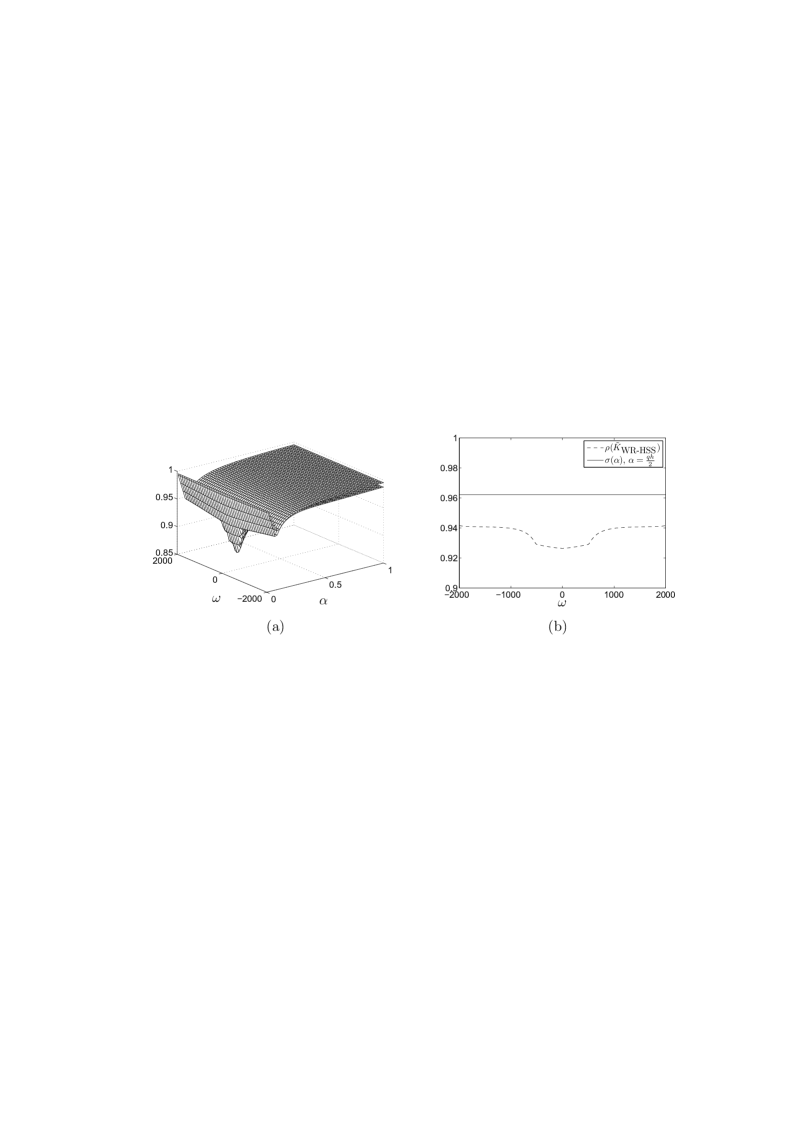
Figure 2: For $q=10$: (a) surfaces of the spectral radius $\rho(\tilde{K}_{\mbox{\tiny WR-HSS}})$ and the upper bound $\sigma(\alpha)$; (b) sectional drawing of the previous surfaces for $\alpha=\frac{qh}{2}$, dashed line for $\rho(\tilde{K}_{\mbox{\tiny WR-HSS}})$ and solid line for $\sigma(\alpha)$.

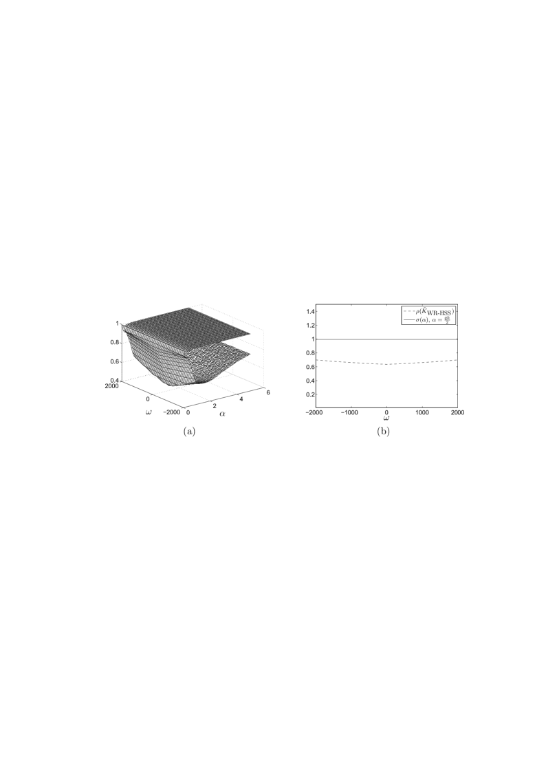
Figure 3: For $q=100$: (a) surfaces of the spectral radius $\rho(\tilde{K}_{\mbox{\tiny WR-HSS}})$ and the upper bound $\sigma(\alpha)$; (b) sectional drawing of the previous surfaces for $\alpha=\frac{qh}{2}$, dashed line for $\rho(\tilde{K}_{\mbox{\tiny WR-HSS}})$ and solid line for $\sigma(\alpha)$.

Figures 1-4 show the surfaces of the spectral radius $\rho(\tilde{K}_{\mbox{\tiny WR-HSS}})$ and the upper bound $\sigma(\alpha)$ on $\omega$-$\alpha$-plane with $\omega_{c}=2000$ for different values of $q$, and the corresponding sectional drawing of the previous surfaces for $\alpha=\frac{qh}{2}$. In addition, the interval of $\alpha$ is determined accordingly. When $q$ is small (e.g., $q=1$ in Figure 1), the surfaces in sub-figure-(a) stick together, and it is difficult to tell the difference between them. Moreover, the corresponding sectional drawing in sub-figure-(b) gives a better illustration of the tiny difference between the spectral radius $\rho(\tilde{K}_{\mbox{\tiny WR-HSS}})$ and the upper bound $\sigma(\alpha)$. When $q$ becomes larger (e.g., $q=1000$ in Figure 4), the surfaces in sub-figure-(a) are wide apart from each other, and the corresponding sectional drawing in sub-figure-(b) also demonstrates a larger difference between the spectral radius $\rho(\tilde{K}_{\mbox{\tiny WR-HSS}})$ and the upper bound $\sigma(\alpha)$.

Table 1 lists the values of the upper bound $\sigma(\alpha)$ and the intervals of the spectral radius $\rho(\tilde{K}_{\mbox{\tiny WR-HSS}})$ with $-\omega_{c}\leq\omega\leq\omega_{c}$ for $\alpha=\frac{qh}{2}$ and different values of $q$. Obviously, the values of the upper bound $\sigma(\alpha)$ are all less than but close to one, which means that the convergence of the WR-HSS method is guaranteed, but the actual convergence rate can not be revealed correctly. In addition, the value of the spectral radius $\rho(\tilde{K}_{\mbox{\tiny WR-HSS}})$ is close to the value of the upper bound $\sigma(\alpha)$ for small $q$, and the value of the spectral radius $\rho(\tilde{K}_{\mbox{\tiny WR-HSS}})$ decreases fast, when the value of $q$ increases.

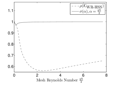
Figure 5: The spectral radius $\rho(\mathcal{K}_{\mbox{\tiny WR-HSS}})$ and the upper bound $\sigma(\alpha)$ with respect to the mesh Reynolds number $\frac{qh}{2}$, dashed line for $\rho(\mathcal{K}_{\mbox{\tiny WR-HSS}})$ and solid line for $\sigma(\alpha)$.

Figure 5 depict the curves of the spectral radius $\rho(\mathcal{K}_{\mbox{\tiny WR-HSS}})$ and the upper bound $\sigma(\alpha)$ with respect to the mesh Reynolds number $\frac{qh}{2}$ with $\alpha=\frac{qh}{2}$. We find that the two curves stay close when the mesh Reynolds number $\frac{qh}{2}$ is small, and when the mesh Reynolds number $\frac{qh}{2}$ increases, the two curves are apart from each other rapidly. Moreover, the curve of the spectral radius $\rho(\mathcal{K}_{\mbox{\tiny WR-HSS}})$ stays below the curve of the upper bound $\sigma(\alpha)$ all the time.

The above observations show that the convergence of the WR-HSS method is unconditionally guaranteed for any positive parameter $\alpha$, the upper bound $\sigma(\alpha)$ is close to the spectral radius $\rho(\mathcal{K}_{\mbox{\tiny WR-HSS}})$ for small $q$, and they are all close to one, which means that $\sigma(\alpha)$ is a good approximation of the spectral radius $\rho(\mathcal{K}_{\mbox{\tiny WR-HSS}})$ when the unsteady elliptic problem has a weak convection term, however, the convergence rate of the WR-HSS method is very slow in this case. When $q$ becomes larger, or say the unsteady elliptic problem has a stronger convection term, the upper bound $\sigma(\alpha)$ keeps close to one, but the spectral radius $\rho(\mathcal{K}_{\mbox{\tiny WR-HSS}})$ is far less than one, which means that the convergence rate of the WR-HSS method is much faster than the upper bound $\sigma(\alpha)$ can reveal.

5.2 The 2-dimensional case

In this subsection, we compare the WR-HSS method with the DGMRES and the WR-SOR method to demonstrate the robustness of the WR-HSS method. We consider the 2-dimensional unsteady elliptic problem

$$\frac{\partial u(x,t)}{\partial t}-\nabla\cdot[a(x,t)\nabla u(x,t)]+\sum_{j=1}^{d}\frac{\partial}{\partial x_{j}}(q(x,t)u(x,t))=0$$

on spatial domain $\Omega$ and time interval $[0,\mbox{T}]$, with positive constant function $a(x,t)=1$ and constant Reynolds function $q(x,t)=q$, and subject to Dirichlet boundary condition. The spatial domain $\Omega$ can be chosen to be a square domain $Q=[0,1]\times[0,1]$ or L-shaped domain $L=Q\setminus G$, with $G=[0,0.5]\times[0,0.5]$. We remark here that we did not observe any difference in the quality of numerical results on the square domain and the L-shaped domain. Thus, we only report the numerical results on square domain.

According to the analysis in Subsection 5.1, the WR-HSS method converges fast for solving the unsteady elliptic problem with strong convection term, thus, $q$ is chosen to be large in the tests in this subsection. When the centered difference scheme is applied to the above unsteady elliptic problem, and the natural lexicographic ordering is employed to the unknowns, we get the unsteady discrete elliptic problem with coefficients

$$B=h^{2}\,I\otimes I\quad\mbox{and}\quad A=I\otimes T_{n}+T_{n}\otimes I,$$

where $T_{n}={\rm tridiag}(-1-\mbox{\it Re},2,-1+\mbox{\it Re})$ with $\mbox{\it Re}=\frac{qh}{2}$ as the mesh Reynolds number. For the convenience of error comparison, the exact solution of the corresponding unsteady discrete elliptic problem is artificially chosen to be

$$x=e^{-t}\,\mbox{\bf 1},$$

where $\mbox{\bf 1}=(1,1,\ldots,1)^{T}$.

In the tests, we choose spatial-grid-size $n=127,255,511,1023$ and time interval $[0,\mbox{T}]=[0,\ell_{t}\times\Delta t]$. The system size on each time level varies from $O(10^{4})$ to $O(10^{6})$. The stopping criterion of the discrete-time WR method on each window is given by

$$\frac{\|r_{\Delta t}^{(k)}\|_{2}}{\|r_{\Delta t}^{(0)}\|_{2}}<\varepsilon,$$

where $\varepsilon$ is a tolerance to control the above stopping criterion. In addition, The stopping criterion of the restarted GMRES($m$) used on each time level of the DGMRES is given by

$$\frac{\|r^{(k)}\|_{2}}{\|r^{(0)}\|_{2}}<\eta,$$

where $\eta$ is a tolerance to control the above stopping criterion.

Tables 2-4 list the experimental feasible interval of iteration parameters for the WR-SOR method and the WR-HSS method for the settings $\Delta t=10^{-4},10^{-5},10^{-6}$, $\ell_{t}=\ell_{t,J}\times J=5\times 1$, $q=2000,3000$ and $n=127,255$. Since these are feasibility tests, the corresponding tolerance is set to be $\varepsilon=0.05$. Here in the tables, “$\tau$” is the parameter of the WR-SOR method, and “$\alpha$” is that of the WR-HSS method. Moreover, “$100+$” means that the tested parameter $\alpha$ exceeds $100$. Obviously, the length of the feasible interval of $\alpha$ is much larger than the length of the feasible interval of $\tau$ in all cases. This means that the iterative parameter of the WR-SOR method is much more sensitive than that of the WR-HSS method. Thus, the WR-HSS method is a better choice for practical aspect. In addition, we observe that the WR-HSS method is not feasible for all positive $\alpha$ in the tests, which contradicts with the result stated in Theorem 3.1 and the observation in Subsection 5.1. The possible reason is that Theorem 3.1 describes the convergence behavior of the continuous-time WR-HSS method, but the actual implemented method is the discrete-time WR-HSS method which is not a HS splitting based method in essential, therefore, not all positive $\alpha$ leads to a convergent discrete-time WR-HSS method.

Tables 5-10 list the numerical results of the WR-HSS method, the WR-SOR method and the DGMRES. The settings of the problems are given by $\Delta t=10^{-4},10^{-5},10^{-6}$, $\ell_{t}=\ell_{t,J}\times J=5\times 5$, $q=2000,3000$ and $n=255,511,1023$. The iterative parameter $\alpha$ of the WR-HSS method is given by $\alpha=\frac{qh}{2}$, the iterative parameter $\tau$ of the WR-SOR method is determined experimentally, and the restarted parameter $m$ used in the DGMRES on each time level is set to be $m=5$ which is the largest $m$ we can use to avoid running out of memory in all cases. In these tables, “IT” represents the average number of iterations on each window of the WR-HSS method and the WR-SOR method, and the average number of iterations (i.e., the average number of matrix-vector product) on each time level of the DGMRES. The maximum number of iterations is $7000$, and “CPU” represents the total computation time on the whole time interval. In addition, the tolerance of the WR-HSS method and the WR-SOR method on each window is fixed to be $\varepsilon=10^{-5}$, and the tolerance of the DGMRES on each time level is given by

$$\eta=\left\{\begin{array}[]{lll}10^{-8},&\mbox{for}&\Delta t=10^{-4},\\ 10^{-9},&\mbox{for}&\Delta t=10^{-5},\\ 10^{-10},&\mbox{for}&\Delta t=10^{-6},\\ \end{array}\right.$$

such that the relative error “ERR” of the approximate solution obtained by the DGMRES can be comparable to that of the approximate solution obtained by the WR-HSS method.

According to Tables 5-10, we find a general fact that the WR-HSS method and the DGMRES outperform the WR-SOR method in the aspects of both the IT and the CPU in all cases. In most cases, the WR-SOR method did not attain the given tolerance $\varepsilon=10^{-5}$ after the maximum number of iterations, i.e., $\mbox{IT}=7000$. In the sequel, we only discuss the numerical behavior of the WR-HSS method and the DGMRES.

For $\Delta t=10^{-4},10^{-5}$ and $q=2000,3000$, the IT of the DGMRES is at least 6 times as many as the IT of the WR-HSS method, and the CPU of the DGMRES is twice the CPU of the WR-HSS method. Obviously, the WR-HSS method is much more efficient than the DGMRES in these cases.

For $\Delta t=10^{-6}$, $q=2000$, $n=255$, both the IT and the CPU of the WR-HSS method are larger than the IT and the CPU of the DGMRES. For $\Delta t=10^{-6}$, $q=2000$, $n=511$ and $\Delta t=10^{-6}$, $q=3000$, $n=255$, the IT of the WR-HSS method is less than the IT of the DGMRES, but the CPU of the WR-HSS method is larger than the CPU of the DGMRES. It seems that the DGMRES is more efficient than the WR-HSS method in these cases, but the fact behind the illusion is that the ERR of the DGMRES is about 100 times as large as the ERR of the WR-HSS method. If we decrease the tolerance $\eta$ of the DGMRES on each time level such that the same ERR as the WR-HSS method attained for the DGMRES in these cases, it can make all the difference.

In all cases in Tables 5-10, the IT and the CPU of the DGMRES both increase proportionally to the increasing proportion of the spatial-grid-size, and they slightly increase with $q$. For $\Delta t=10^{-4},10^{-5}$ and $q=2000,3000$, the increasing behavior of the WR-HSS method is similar to that of the DGMRES. However, for $\Delta t=10^{-6}$ and $q=2000,3000$, the surprising fact is that the IT of the WR-HSS method is slightly decreasing with the increasing spatial-grid-size.

Tables 11-13 list the results of the numerical solution of the 2-dimensional unsteady elliptic problem on the long time interval by using the WR-HSS method for the settings $[0,\mbox{T}]=[0,1]$, $\Delta t=10^{-3},10^{-4},10^{-5}$, $\ell_{t}=\ell_{t,J}\times J=5\times 200,5\times 2000,5\times 20000$, $q=2000,3000$, and $n=127,255$. The iterative parameter $\alpha$ of the WR-HSS method is given by $\alpha=\frac{qh}{2}$, and the tolerance of the WR-HSS method on each window is given by $\varepsilon=10^{-5}$. In these tables, we find that the IT of the WR-HSS method increases both with $q$ and with the spatial-grid-size $n+1$. However, the IT of the WR-HSS method decreases fast with the time-step-size $\Delta t$. Moreover, the ERR of the WR-HSS method on long time interval remains the same orders of magnitude as the ERR of the WR-HSS method on short time interval, e.g., in the cases $\Delta t=10^{-4},10^{-5}$, $q=2000,3000$ and $n=255$.

6 Conclusions

In this paper, we propose a two-step operator splitting method based on the HS splitting of the differential operator for solving the unsteady discrete elliptic problem, i.e., WR-HSS method. The theoretical analysis and the numerical results both suggest that the WR-HSS method is effective for handling the unsteady discrete elliptic problem.

The advantages of the WR-HSS method can be addressed in two main aspects. Firstly, compared with other analytical methods (such as the WR-SOR method), the WR-HSS method converges unconditionally to the solution of the system of linear differential equations, and there is an easy implemented strategy for computing the iterative parameter. For the WR-SOR method, however, the length of the feasible interval of the iterative parameter is small, and the practical iterative parameter is hard to determine. Secondly, compared with the classical time-stepping methods (such as the DGMRES method) who deal with the original system of linear differential equations directly, the WR-HSS method splits the original difficult system of linear differential equations into two easy sub-systems which are much easier to resolve.

In practical aspect, the WR-HSS method must be implemented discretely, i.e., the discrete-time WR-HSS method, but the theoretical analysis in this paper are only concentrated on the continuous-time WR-HSS method, therefore, our future work should be the discussion on the convergence property of the discrete-time method, and the relationship between the discrete-time and continuous-time method.

Figure 1: For $q=1$: (a) surfaces of the spectral radius $\rho(\tilde{K}_{\mbox{\tiny WR-HSS}})$ and the upper bound $\sigma(\alpha)$; (b) sectional drawing of the previous surfaces for $\alpha=\frac{qh}{2}$, dashed line for $\rho(\tilde{K}_{\mbox{\tiny WR-HSS}})$ and solid line for $\sigma(\alpha)$.

Figure 4: For $q=1000$: (a) surfaces of the spectral radius $\rho(\tilde{K}_{\mbox{\tiny WR-HSS}})$ and the upper bound $\sigma(\alpha)$; (b) sectional drawing of the previous surfaces for $\alpha=\frac{qh}{2}$, dashed line for $\rho(\tilde{K}_{\mbox{\tiny WR-HSS}})$ and solid line for $\sigma(\alpha)$.

Table 1: Values of the upper bound $\sigma(\alpha)$ and the spectral radius $\rho(\tilde{K}_{\mbox{\tiny WR-HSS}})$ with $-\omega_{c}\leq\omega\leq\omega_{c}$ for $\alpha=\frac{qh}{2}$.

	$\sigma(\alpha)$	$\rho(\tilde{K}_{\mbox{\tiny WR-HSS}})$
$q=1$	0.9962	(0.9923, 0.9958)
$q=10$	0.9622	(0.9264, 0.9417)
$q=100$	0.9939	(0.6339, 0.6976)
$q=1000$	0.9994	(0.6444, 0.6515)

Table 2: The interval of feasible iteration parameter of the WR-SOR method and the WR-HSS method: $\Delta t=10^{-4}$.

	$q=2000$		$q=3000$
	$r=n^{2},n=127$	$r=n^{2},n=255$	$r=n^{2},n=127$	$r=n^{2},n=255$
WR-SOR, $\tau$	(0.0019, 0.2294)	(0.0019, 0.4097)	(0.0019, 0.1582)	(0.0019, 0.2924)
WR-HSS, $\alpha$	(0.9766, 100+)	(0.9766, 100+)	(1.4648, 100+)	(0.7324, 100+)

Table 3: The interval of feasible iteration parameter of the WR-SOR method and the WR-HSS method: $\Delta t=10^{-5}$.

	$q=2000$		$q=3000$
	$r=n^{2},n=127$	$r=n^{2},n=255$	$r=n^{2},n=127$	$r=n^{2},n=255$
WR-SOR, $\tau$	(0.0019, 0.2540)	(0.0019, 0.4287)	(0.0019, 0.1707)	(0.0019, 0.3024)
WR-HSS, $\alpha$	(0.9766, 100+)	(0.9766, 100+)	(0.7324, 100+)	(0.7324, 100+)

Table 4: The interval of feasible iteration parameter of the WR-SOR method and the WR-HSS method: $\Delta t=10^{-6}$.

	$q=2000$		$q=3000$
	$r=n^{2},n=127$	$r=n^{2},n=255$	$r=n^{2},n=127$	$r=n^{2},n=255$
WR-SOR, $\tau$	(0.0019, 2.6814)	(0.0019, 0.7862)	(0.0019, 0.6169)	(0.0019, 0.4448)
WR-HSS, $\alpha$	(5.1270, 100+)	(1.9531, 100+)	(5.1270, 100+)	(1.4648, 100+)

Table 5: The number of iterations, computation time and the relative errors of the approximate solutions for different methods on time interval $[0,\ell_{t,J}\times J\times\Delta t]=[0,5\times 5\times\Delta t]$: $\Delta t=10^{-4}$ and $q=2000$.

	$r=n^{2},n=255$			$r=n^{2},n=511$			$r=n^{2},n=1023$
	IT	CPU	ERR	IT	CPU	ERR	IT	CPU	ERR
WR-HSS	106	188.7031	6.3E-08	155	1348.3750	7.0E-08	272	9727.0313	1.2E-07
WR-SOR	7000	1254.5313	5.1E-04	7000	4878.5469	3.7E-03	7000	18436.4375	2.1E-03
DGMRES	649	337.9844	1.3E-07	1096	2490.8594	2.3E-07	2107	19215.8281	1.7E-07

Table 6: The number of iterations, computation time and the relative errors of the approximate solutions for different methods on time interval $[0,\ell_{t,J}\times J\times\Delta t]=[0,5\times 5\times\Delta t]$: $\Delta t=10^{-4}$ and $q=3000$.

	$r=n^{2},n=255$			$r=n^{2},n=511$			$r=n^{2},n=1023$
	IT	CPU	ERR	IT	CPU	ERR	IT	CPU	ERR
WR-HSS	126	226.6406	5.8E-08	171	1483.0000	8.5E-08	281	10086.8125	6.7E-08
WR-SOR	7000	1310.3281	3.1E-04	7000	4878.7031	3.5E-03	7000	18430.7344	3.4E-03
DGMRES	712	372.2188	2.7E-07	1192	2711.0938	1.1E-07	2149	19590.9063	3.3E-07

Table 7: The number of iterations, computation time and the relative errors of the approximate solutions for different methods on time interval $[0,\ell_{t,J}\times J\times\Delta t]=[0,5\times 5\times\Delta t]$: $\Delta t=10^{-5}$ and $q=2000$.

	$r=n^{2},n=255$			$r=n^{2},n=511$			$r=n^{2},n=1023$
	IT	CPU	ERR	IT	CPU	ERR	IT	CPU	ERR
WR-HSS	30	54.8281	3.2E-09	47	406.3438	8.1E-09	91	3263.3438	7.4E-09
WR-SOR	4037	755.7500	1.1E-08	7000	4877.6406	1.4E-05	7000	18427.1875	4.7E-06
DGMRES	208	107.0313	4.7E-08	410	927.1875	6.9E-08	822	7466.7813	5.2E-08

Table 8: The number of iterations, computation time and the relative errors of the approximate solutions for different methods on time interval $[0,\ell_{t,J}\times J\times\Delta t]=[0,5\times 5\times\Delta t]$: $\Delta t=10^{-5}$ and $q=3000$.

	$r=n^{2},n=255$			$r=n^{2},n=511$			$r=n^{2},n=1023$
	IT	CPU	ERR	IT	CPU	ERR	IT	CPU	ERR
WR-HSS	45	80.8125	3.7E-09	69	592.3594	1.2E-08	132	4736.0313	1.2E-08
WR-SOR	3858	722.9531	1.4E-08	7000	4886.3906	1.7E-05	7000	18455.6094	2.1E-04
DGMRES	324	166.7188	5.9E-08	608	1376.5000	6.7E-08	1202	10952.3438	6.6E-08

Table 9: The number of iterations, computation time and the relative errors of the approximate solutions for different methods on time interval $[0,\ell_{t,J}\times J\times\Delta t]=[0,5\times 5\times\Delta t]$: $\Delta t=10^{-6}$ and $q=2000$.

	$r=n^{2},n=255$			$r=n^{2},n=511$			$r=n^{2},n=1023$
	IT	CPU	ERR	IT	CPU	ERR	IT	CPU	ERR
WR-HSS	35	63.7500	5.8E-11	17	150.1563	6.0E-11	14	487.7031	5.9E-10
WR-SOR	98	18.8750	3.7E-10	1723	1202.9375	2.7E-10	1561	4166.5469	1.6E-10
DGMRES	28	12.4531	7.8E-09	49	103.4063	6.0E-09	93	824.5313	3.7E-09

Table 10: The number of iterations, computation time and the relative errors of the approximate solutions for different methods on time interval $[0,\ell_{t,J}\times J\times\Delta t]=[0,5\times 5\times\Delta t]$: $\Delta t=10^{-6}$ and $q=3000$.

	$r=n^{2},n=255$			$r=n^{2},n=511$			$r=n^{2},n=1023$
	IT	CPU	ERR	IT	CPU	ERR	IT	CPU	ERR
WR-HSS	23	41.0000	6.2E-11	13	114.1406	2.8E-10	15	547.4531	2.0E-10
WR-SOR	427	81.5469	4.5E-10	1710	1199.2969	3.5E-10	6853	18363.9219	2.4E-10
DGMRES	38	18.2500	2.6E-09	69	150.5313	3.1E-09	133	1204.5625	2.1E-09

Table 11: The number of iterations and the relative errors of the approximate solutions for WR-HSS method on time interval $[0,1]$: $\Delta t=10^{-3}$, $\ell_{t}=\ell_{t,J}\times J=5\times 200$.

	$q=2000$		$q=3000$
	$r=n^{2},n=127$	$r=n^{2},n=255$	$r=n^{2},n=127$	$r=n^{2},n=255$
IT	97	116	116	133
ERR	1.0E-06	7.8E-07	7.0E-07	7.8E-07

Table 12: The number of iterations and the relative errors of the approximate solutions for WR-HSS method on time interval $[0,1]$: $\Delta t=10^{-4}$, $\ell_{t}=\ell_{t,J}\times J=5\times 2000$.

	$q=2000$		$q=3000$
	$r=n^{2},n=127$	$r=n^{2},n=255$	$r=n^{2},n=127$	$r=n^{2},n=255$
IT	86	106	108	126
ERR	9.9E-08	6.3E-08	5.4E-08	5.8E-08

Table 13: The number of iterations and the relative errors of the approximate solutions for WR-HSS method on time interval $[0,1]$: $\Delta t=10^{-5}$, $\ell_{t}=\ell_{t,J}\times J=5\times 20000$.

	$q=2000$		$q=3000$
	$r=n^{2},n=127$	$r=n^{2},n=255$	$r=n^{2},n=127$	$r=n^{2},n=255$
IT	25	30	38	45
ERR	7.7E-09	6.3E-09	5.5E-09	4.8E-09

References

• [1] Z.Z. Bai, Optimal parameters in the HSS-like methods for saddle-point problems, Numer. Linear Algebra Appl. 16(2009) 447-479.
• [2] Z.Z. Bai, M. Benzi, F. Chen, Modified HSS iteration methods for a class of complex symmetric linear systems, Comput. 87(2010) 93-111.
• [3] Z.Z. Bai, M. Benzi, F. Chen, On preconditioned MHSS iteration methods for complex symmetric linear systems, Numer. Algorithms 56(2011) 297-317.
• [4] Z.Z. Bai, M. Benzi, F. Chen, Z.Q. Wang, Preconditioned MHSS iteration methods for a class of block two-by-two linear systems with applications to distributed control problems, IMA J. Numer. Anal. 33(2013) 343-369.
• [5] Z.Z. Bai, G.H. Golub, Accelerated Hermitian and skew-Hermitian splitting iteration methods for saddle-point problems, IMA J. Numer. Anal. 27(2007) 1-23.
• [6] Z.Z. Bai, G.H. Golub, C.K. Li, Optimal parameter in Hermitian and skew-Hermitian splitting method for certain two-by-two block matrices, SIAM J. Sci. Comput. 28(2006) 583-603.
• [7] Z.Z. Bai, G.H. Golub, C.K. Li, Convergence properties of preconditioned Hermitian and skew-Hermitian splitting methods for non-Hermitian positive semidefinite matrices, Math. Comput. 76(2007) 287-298.
• [8] Z.Z. Bai, G.H. Golub, L.Z. Lu, J.F. Yin, Block triangular and skew-Hermitian splitting methods for positive-definite linear systems, SIAM J. Sci. Comput. 26(2005) 844-863.
• [9] Z.Z. Bai, G.H. Golub, M.K. Ng, Hermitian and skew-Hermitian splitting methods for non-Hermitian positive definite linear systems, SIAM J. Matrix Anal. Appl. 24(2003) 603-626.
• [10] Z.Z. Bai, G.H. Golub, M.K. Ng, On successive overrelaxation acceleration of the Hermitian and skew-Hermitian splitting iterations, Numer. Linear Algebra Appl. 14(2007) 319-335.
• [11] Z.Z. Bai, G.H. Golub, M.K. Ng, On inexact Hermitian and skew-Hermitian splitting methods for non-Hermitian positive definite linear systems, Linear Algebra Appl. 428(2008) 413-440.
• [12] Z.Z. Bai, G.H. Golub, J.Y. Pan, Preconditioned Hermitian and skew-Hermitian splitting methods for non-Hermitian positive semidefinite linear systems, Numer. Math. 98(2004) 1-32.
• [13] Z.Z. Bai, M.K. Ng, J.Y. Pan, Alternating splitting waveform relaxation method and its successive overrelaxation acceleration, Comput. Math. Appl. 49(2005) 157-170.
• [14] D. Bertaccini, G.H. Golub, S.S. Capizzano, C.T. Possio, Preconditioned HSS methods for the solution of non-Hermitian positive definite linear systems and applications to the discrete convection-diffusion equation, Numer. Math. 99(2005) 441-484.
• [15] S.L. Campbell, Singular Systems of Differential Equations, Pitman Advanced Publishing Program, London and Melbourne, 1980.
• [16] J. Douglas Jr., H.H. Rachford Jr., Alternating direction methods for three space variables, Numer. Math. 4(1956) 41-63.
• [17] H.C. Elman, G.H. Golub, Iterative methods for cyclically reduced non-self-adjoint linear systems, Math. Comput. 54(1990) 671-700.
• [18] H.C. Elman, G.H. Golub, Iterative methods for cyclically reduced non-self-adjoint linear systems II, Math. Comput. 56(1990) 215-242.
• [19] H.C. Elman, D.J. Silvester, A.J. Wathen, Finite Elements and Fast Iterative Solvers: with Applications in Incompressible Fluid Dynamics, Oxford University Press, New York, 2005.
• [20] W. Hackbusch, Multi-Grid Mehtods and Applications, Springer-Verlag, Berlin Heidelberg, 1985.
• [21] H. Hochstadt, Integral Equations, John Wiley & Sons, New York, 1989.
• [22] J. Janssen, S. Vandewalle, On SOR waveform relaxation methods, SIAM J. Numer. Anal. 34(1997) 2456-2481.
• [23] Y.L. Jiang, Waveform Relaxation Methods, Science Press, Beijing, 2009.
• [24] E. Lelarasmee, A. Ruheli, A.L. Sangiovanni-Vincentelli, The waveform relaxation method for time-domain analysis of large scale integrated circuits, IEEE Trans. Comput.-Aided Des. Integr. Circuits Syst. CAD-1(1982) 131-145.
• [25] F.L. Lewis, A survey of linear singular systems, Circuits Syst. Signal Process. 5(1986) 3-36.
• [26] U. Miekkala, O. Nevanlinna, Convergence of dynamic iteration methods for initial value problems, SIAM J. Sci. Stat. Comput. 8(1987) 459-482.
• [27] J.Y. Pan, Z.Z. Bai, On the convergence of waveform relaxation methods for linear initial value problems, J. Comput. Math. 22(2004) 681-698.
• [28] J.Y. Pan, Z.Z. Bai, M.K. Ng, Two-step waveform relaxation methods for implicit linear initial value problems, Numer. Linear Algebra Appl. 12(2005) 293-304.
• [29] J. Wang, Z.Z. Bai, Convergence analysis of two-stage waveform relaxation method for the initial value problems, Appl. Math. Comput. 172(2006) 797-808.
Refer to caption