Discrete-Time
Accelerated Block Successive Overrelaxation Methods
for Time-Dependent Stokes Equations

Abstract

To further study the application of waveform relaxation methods in fluid dynamics in actual computation, this paper provides a general theoretical analysis of discrete-time waveform relaxation methods for solving linear DAEs. A class of discrete-time waveform relaxation methods, named discrete-time accelerated block successive overrelaxation (DABSOR) methods, is proposed for solving linear DAEs derived from discretizing time-dependent Stokes equations in space by using “Method of Lines”. The analysis of convergence property and optimality of the DABSOR method are presented in detail. The theoretical results and the efficiency of the DABSOR method are verified by numerical experiments.

Keywords: differential-algebraic equations, linear convolution operator, saddle-structure, time-dependent Stokes equation, waveform relaxation method.

AMS(MOS) Subject Classifications: 65F10, 65L80, 65N06, 65N22, 65N40; CR: G1.3.

1 Introduction

We consider the numerical solution for time-dependent Stokes equations of the form

$$\left\{\begin{array}[]{rcll}\frac{\partial\vec{u}}{\partial t}-\nu\nabla^{2}\vec{u}+\nabla p&=&0&\mbox{in}\enskip\Omega\times\mathbb{R}_{+},\\ \nabla\cdot\vec{u}&=&0&\mbox{in}\enskip\Omega\times\mathbb{R}_{+},\\ \vec{u}&=&0&\mbox{on}\enskip\partial\Omega\times\mathbb{R}_{+},\\ \vec{u}&=&\vec{u}_{0}&\mbox{on}\enskip\Omega\times\{0\},\\ \end{array}\right.$$ (1.5)

with certain initial and boundary conditions in $d$-dimensional locally Lipschitz bounded domain $\Omega\subset\mathbb{R}^{d}$ ($d=2$ or $3$). By adopting the idea of “Method of Lines”, equations (1.5) are discretized in space to obtain the following saddle-structured differential-algebraic equations (DAEs)

$$\mathcal{B}\dot{z}(t)+\mathcal{A}z(t)=b(t),\quad z(0)=z_{0},$$ (1.6)

where $z(t)=\left(x(t)^{T},y(t)^{T}\right)^{T}$ with $x(t)$ and $y(t)$ related to velocity and pressure in equations (1.5) respectively, $\mathcal{B}$ and $\mathcal{A}$ are block two-by-two square matrices of the form

$$\mathcal{B}=\left(\begin{array}[]{cc}I&0\\ 0&0\end{array}\right)\quad\mbox{and}\quad\mathcal{A}=\left(\begin{array}[]{cc}A&B\\ -B^{T}&0\end{array}\right),$$

with $A\in\mathbb{R}^{r\times r}$ being a symmetric positive definite matrix, $B\in\mathbb{R}^{r\times l}$ a full column-rank matrix, and $I\in\mathbb{R}^{r\times r}$ the identity matrix. Here, $r$ and $l$ are known positive integers.

In [3], a class of continuous-time waveform relaxation methods for solving linear DAEs (1.6) has been proposed by the application of generalized successive overrelaxation (GSOR) technique [1]. Previous continuous-time waveform relaxation methods, for solving ODEs [2, 8, 9, 16, 18, 19, 20, 21] and DAEs [3, 4, 12, 14], can be regarded as extensions of the classical iterative methods for solving system of algebraic equations with iterating space changing from $\mathbb{R}^{n}$ to the waveform space. Since the analytical operations and exact expressions of waveforms are required in each iterative step, the continuous-time waveform relaxation methods are unlikely to be practical numerical methods, but only be of theoretical interest.

In actual numerical solution for linear DAEs (1.6), the continuous-time waveform relaxation methods in [3] are replaced by a class of discrete-time waveform relaxation methods, named discrete-time accelerated block successive overrelaxation (DABSOR) methods. This paper studies the general theory of discrete-time waveform relaxation methods for solving linear DAEs and the special case of the DABSOR method. In previous discrete-time waveform relaxation methods [8, 10, 11], the waveforms and the linear differential operators in continuous-time waveform relaxation methods are replaced by vector sequences and discrete linear convolution operators respectively. Here, the vector sequences are composed of values of waveforms on each time level, and the discrete linear convolution operators are closely related to the discretizations of the linear differential operators by different time stepping schemes [5, 7] in each iterative step of the continuous-time waveform relaxation methods for solving linear DAEs (1.6).

The structure of this paper is as follows. It is started in Section 2 by briefly reviewing the spectral properties of the discrete linear convolution operator. The general framework of the discrete-time waveform relaxation methods and the corresponding discrete linear convolution operator form are stated in Section 3. In Section 4, the convergence properties of the discrete linear convolution operator derived from the discrete-time waveform relaxation methods for solving linear DAEs are analyzed on both finite and infinite time interval. The DABSOR method without or with windowing technique is constructed in Section 5, and the convergence domain of relaxation parameters and the optimality of the DABSOR method are also presented here. The numerical results are listed in Section 6, which is followed by the concluding remarks in Section 7.

2 Spectral Properties of Discrete Linear Convolution Operator

Consider the following iterative scheme

$$z_{\text{\tiny$\triangle t$}}^{(k)}=\mathcal{H}_{\text{\tiny$\triangle t$}}z_{\text{\tiny$\triangle t$}}^{(k-1)}+\varphi_{\text{\tiny$\triangle t$}},$$ (2.1)

where the subscript $\triangle t$ is the notation of vector sequences, e.g. $z_{\text{\tiny$\triangle t$}}^{(k)}=\{z_{i}^{(k)}\}_{i=0}^{L-1}$, where $L$ (possibly infinite) is the number of components. Each $d$-dimensional component denotes the approximate solution of a $d$-dimensional ODEs or DAEs on a time level. Operator $\mathcal{H}_{\text{\tiny$\triangle t$}}$ is a discrete linear convolution operator with matrix-valued kernel $h_{\text{\tiny$\triangle t$}}$,

$$(\mathcal{H}_{\text{\tiny$\triangle t$}}z_{\text{\tiny$\triangle t$}})_{j}=(h_{\text{\tiny$\triangle t$}}\star z_{\text{\tiny$\triangle t$}})_{j}=\sum_{i=0}^{j}h_{j-i}z_{i},\quad j=0,\ldots,L-1.$$ (2.2)

The convergence properties of operator $\mathcal{H}_{\text{\tiny$\triangle t$}}$ are analyzed in the Banach spaces of $\mathbb{C}^{d}$-valued $p$-summable sequences of length $L$, $l_{p}(L;\mathbb{C}^{d})$, or $l_{p}(L)$ for short, with norms given by

$$\|z_{\text{\tiny$\triangle t$}}\|_{p}=\left\{\begin{array}[]{ll}\root p \of{\sum_{i=0}^{L-1}\|z_{i}\|^{p}}&1\leq p<\infty,\\ \sup\limits_{0\leq i<L}\{\|z_{i}\|\}&p=\infty,\end{array}\right.$$ (2.5)

with $\|\cdot\|$ any prescribed $\mathbb{C}^{d}$ vector norm. It is known that the iterative scheme (2.1) is convergent if and only if the spectral radius of the discrete linear convolution operator $\mathcal{H}_{\text{\tiny$\triangle t$}}$, denoted by $\rho(\mathcal{H}_{\text{\tiny$\triangle t$}})$, is smaller than one. The following two lemmas provide specific descriptions of $\rho(\mathcal{H}_{\text{\tiny$\triangle t$}})$ on both finite and infinite time intervals [8].

Lemma 2.1

Consider $\mathcal{H}_{\text{\tiny$\triangle t$}}$ as an operator in $l_{p}(L)$, with $1\leq p\leq\infty$ and $L$ finite. Then, $\mathcal{H}_{\text{\tiny$\triangle t$}}$ is a bounded operator and

$$\rho(\mathcal{H}_{\text{\tiny$\triangle t$}})=\rho(h_{0})=\rho(\text{\bf H}_{\text{\tiny$\triangle t$}}(\infty)),$$

with $\text{\bf H}_{\text{\tiny$\triangle t$}}(s)=\sum_{i=0}^{L-1}h_{i}s^{-i}$ the discrete Laplace transform of $h_{\text{\tiny$\triangle t$}}$.

Lemma 2.2

Suppose that $h_{\text{\tiny$\triangle t$}}\in\l_{1}(\infty)$, and consider $\mathcal{H}_{\text{\tiny$\triangle t$}}$ as an operator in $l_{p}(\infty)$, with $1\leq p\leq\infty$. Then, $\mathcal{H}_{\text{\tiny$\triangle t$}}$ is a bounded operator and

$$\rho(\mathcal{H}_{\text{\tiny$\triangle t$}})=\max_{|s|\geq 1}\rho(\text{\bf H}_{\text{\tiny$\triangle t$}}(s))=\max_{|s|=1}\rho(\text{\bf H}_{\text{\tiny$\triangle t$}}(s)),$$

with $\text{\bf H}_{\text{\tiny$\triangle t$}}(s)=\sum_{i=0}^{\infty}h_{i}s^{-i}$ the discrete Laplace transform of $h_{\text{\tiny$\triangle t$}}$.

3 Discrete-Time Waveform Relaxation Methods

The continuous-time waveform relaxation methods for solving the linear DAEs (1.6) are defined by spliting the square matrices $\mathcal{B}$ and $\mathcal{A}\in\mathbb{R}^{(r+l)\times(r+l)}$ into

$$\mathcal{B}=M_{\mathcal{B}}-N_{\mathcal{B}}\quad\mbox{and}\quad\mathcal{A}=M_{\mathcal{A}}-N_{\mathcal{A}},$$

respectively. Then the corresponding iterative scheme is of the form

$$\left\{\begin{array}[]{l}M_{\mathcal{B}}\dot{z}^{(k)}+M_{\mathcal{A}}z^{(k)}=N_{\mathcal{B}}\dot{z}^{(k-1)}+N_{\mathcal{A}}z^{(k-1)}+b,\\ z^{(k)}(0)=z_{0}.\end{array}\right.$$ (3.3)

Furthermore, iterative scheme (3.3) can be rewritten explicitly

$$z^{(k)}=\mathcal{K}(z^{(k-1)})+\Phi(b),$$ (3.4)

where

$$\mathcal{K}(z)=(\mathcal{L}^{-1}(sM_{\mathcal{B}}+M_{\mathcal{A}})^{-1}(sN_{\mathcal{B}}+N_{\mathcal{A}})\mathcal{L})(z)$$

and

$$\Phi(b)=(\mathcal{L}^{-1}(sM_{\mathcal{B}}+M_{\mathcal{A}})^{-1}\mathcal{L})(b).$$

Here, $\mathcal{L}$ denotes the continuous Laplace transform. It has been shown in [4] that

$$\rho(\mathcal{K})=\sup_{\Re(s)=\sigma}\rho\left(\text{\bf K}(s)\right),$$ (3.5)

where

$$\text{\bf K}(s)=(sM_{\mathcal{B}}+M_{\mathcal{A}})^{-1}(sN_{\mathcal{B}}+N_{\mathcal{A}}).$$ (3.6)

Applying a linear multistep formula to the continuous-time waveform relaxation scheme (3.3) leads to the following discrete-time waveform relaxation scheme

$$\frac{1}{\triangle t}\sum_{j=0}^{\nu}\alpha_{j}M_{\mathcal{B}}z_{n+j}^{(k)}+\sum_{j=0}^{\nu}\beta_{j}M_{\mathcal{A}}z_{n+j}^{(k)}=\\ \frac{1}{\triangle t}\sum_{j=0}^{\nu}\alpha_{j}N_{\mathcal{B}}z_{n+j}^{(k-1)}+\sum_{j=0}^{\nu}\beta_{j}N_{\mathcal{A}}z_{n+j}^{(k-1)}+\sum_{j=0}^{\nu}\beta_{j}b_{n+j},\quad n\geq 0.$$ (3.7)

Assume that the $\nu$ starting values of the linear multistep formula are known, hence it is not necessary to iterate on the $\nu$ starting values, i.e. $z_{j}^{(k)}=z_{j}^{(k-1)}=z_{j}$, for $j<\nu$. Due to the numerical stability, the rest of this paper is concentrated on the application of implicit linear multistep formulae, i.e. $\beta_{\nu}\neq 0$.

For every nonnegative integer $n$, system of linear equations (3.7) can be solved uniquely if and only if the following condition is satisfied

$$\frac{\alpha_{\nu}}{\beta_{\nu}}\notin{\rm sp}(M_{\mathcal{B}},-\triangle tM_{\mathcal{A}}),$$ (3.8)

where ${\rm sp}(\cdot)$ represents the spectrum of the matrix pencil $(M_{\mathcal{B}},-\triangle tM_{\mathcal{A}})$. Subsequently, the above condition (3.8) is referred to as the discrete solvability condition.

Similar to the calculation in [18], the iterative scheme (3.7) can be rewritten into the following discrete linear convolution operator form

$$z_{\text{\tiny$\triangle t$}}^{(k)}=\mathcal{K}_{\text{\tiny$\triangle t$}}z_{\text{\tiny$\triangle t$}}^{(k-1)}+\varphi_{\text{\tiny$\triangle t$}}.$$ (3.9)

Since it does not iterate on the $\nu$ starting values, a slight change is made on the subscript $\triangle t$ here, that is

$$z_{\text{\tiny$\triangle t$}}^{(k)}=\{z_{\nu+i}^{(k)}\}_{i=0}^{L-1}.$$ (3.10)

In order to analyze the properties of the discrete linear convolution operator $\mathcal{K}_{\text{\tiny$\triangle t$}}$, the computational error on the $k$-th iteration of (3.7) is denoted by $e_{n}^{(k)}=z_{n}^{(k)}-z_{n}$, where $z_{n}$ is the exact solution of the disrete system derived from the discretezation of linear DAEs (1.6) by the corresponding linear multistep formula. Let $C_{j}=\frac{1}{\triangle t}\alpha_{j}M_{\mathcal{B}}+\beta_{j}M_{\mathcal{A}}$ and $D_{j}=\frac{1}{\triangle t}\alpha_{j}N_{\mathcal{B}}+\beta_{j}N_{\mathcal{A}}$, based on (3.7), we get

$$\sum_{j=0}^{\nu}C_{j}e_{n+j}^{(k)}=\sum_{j=0}^{\nu}D_{j}e_{n+j}^{(k-1)},\quad n\geq 0.$$ (3.11)

Combine the first $L$ equations, introduce vector notation $E^{(k)}=\left({e_{\nu}^{(k)}}^{T},{e_{\nu+1}^{(k)}}^{T},\ldots,{e_{L+\nu-1}^{(k)}}^{T}\right)^{T}$, and note that $e_{j}^{(k)}=e_{j}^{(k-1)}=0$, $j<\nu$, we have

$$E^{(k)}=C^{-1}DE^{(k-1)}.$$

Here, matrices $C$ and $D$ are $L\times L$-block lower triangular Toeplitz matrices with $\nu+1$ constant diagonals. It follows that matrix $C^{-1}D$ is also a $L\times L$-block lower triangular Toeplitz matrix with $\nu+1$ constant diagonals. Hence, $\mathcal{K}_{\text{\tiny$\triangle t$}}$ is a discrete linear convolution operator on the Banach space $l_{p}(L)$.

The discrete Laplace transform of the convolution kernel $\kappa_{\text{\tiny$\triangle t$}}$ of the discrete linear convolution operator $\mathcal{K}_{\text{\tiny$\triangle t$}}$ can be obtained by applying discrete Laplace transform to equation (3.11). If $\tilde{e}_{\text{\tiny$\triangle t$}}^{(k)}(s)$ denotes the discrete Laplace transform of $e_{\text{\tiny$\triangle t$}}^{(k)}$, we find

$$\tilde{e}_{\text{\tiny$\triangle t$}}^{(k)}(s)=\text{\bf K}_{\text{\tiny$\triangle t$}}(s)\tilde{e}_{\text{\tiny$\triangle t$}}^{(k-1)}(s),$$

with discrete Laplace transform of the convolution kernel $\kappa_{\text{\tiny$\triangle t$}}$ given by

$$\text{\bf K}_{\text{\tiny$\triangle t$}}(s)=(a(s)M_{\mathcal{B}}+\triangle tb(s)M_{\mathcal{A}})^{-1}(a(s)N_{\mathcal{B}}+\triangle tb(s)N_{\mathcal{A}}).$$ (3.12)

where $a(s)=\sum_{j=0}^{\nu}\alpha_{j}s^{j}$ and $b(s)=\sum_{j=0}^{\nu}\beta_{j}s^{j}$. By comparison to (3.6), we have the following relation

$$\text{\bf K}_{\text{\tiny$\triangle t$}}(s)=\text{\bf K}\left(\frac{1}{\triangle t}\frac{a}{b}(s)\right).$$ (3.13)

4 Convergence Analysis of $\mathcal{K}_{\text{\tiny$\triangle t$}}$

The convergence property of the discrete linear convolution operator $\mathcal{K}_{\text{\tiny$\triangle t$}}$ on finite time interval is an immediate result of Lemma 2.1. The result can be stated as the following theorem straightforwardly.

Theorem 4.1

Assume that the discrete solvability condition (3.8) is satisfied, and consider $\mathcal{K}_{\text{\tiny$\triangle t$}}$ as a discrete linear convolution operator in $l_{p}(L)$, with $1\leq p\leq\infty$ and $L$ finite. Then, $\mathcal{K}_{\text{\tiny$\triangle t$}}$ is bounded and

$$\rho(\mathcal{K}_{\text{\tiny$\triangle t$}})=\rho\left(\text{\bf K}\left(\frac{1}{\triangle t}\frac{\alpha_{\nu}}{\beta_{\nu}}\right)\right).$$ (4.1)

However, the convergence property of the discrete linear convolution operator $\mathcal{K}_{\text{\tiny$\triangle t$}}$ on infinite time interval is a little bit complicated, thus, an important lemma is introduced.

Lemma 4.1

Assume that the discrete solvability condition (3.8) is satisfied. Let $b(z)\neq 0$, $\forall$ $|z|=1$. If ${\rm sp}(M_{\mathcal{B}},-\triangle tM_{\mathcal{A}})\subset\text{\r{S}}$ and $\infty\in S$, then $\mathcal{K}_{\text{\tiny$\triangle t$}}$ is bounded in $l_{p}(\infty)$. Where $S$ represents the absolute stability region of the corresponding linear multistep formula, and S̊ denotes the interior of $S$.

Proof: According to the Young’s inequality for discrete convolution product [6], we only need to prove that the kernel $\kappa_{\text{\tiny$\triangle t$}}$ of the discrete convolution operator $\mathcal{K}_{\text{\tiny$\triangle t$}}$ is a $l_{1}$-sequence.

Denote $\theta^{(-1)}_{\text{\tiny$\triangle t$}}$, $\theta_{\text{\tiny$\triangle t$}}$ and $\zeta_{\text{\tiny$\triangle t$}}$ as the sequences whose discrete Laplace transforms are $(a(s)M_{\mathcal{B}}+\triangle tb(s)M_{\mathcal{A}})^{-1}s^{k}$, $s^{-k}(a(s)M_{\mathcal{B}}+\triangle tb(s)M_{\mathcal{A}})$, and $s^{-k}(a(s)N_{\mathcal{B}}+\triangle tb(s)N_{\mathcal{A}})$, respectively. Note that the discrete Laplace transform of $\kappa_{\text{\tiny$\triangle t$}}$ satisfies (3.12), then

$$\kappa_{\text{\tiny$\triangle t$}}=\theta^{(-1)}_{\text{\tiny$\triangle t$}}\star\zeta_{\text{\tiny$\triangle t$}}.$$

Hence, $\kappa_{\text{\tiny$\triangle t$}}$ is a $l_{1}$-sequence if $\theta^{(-1)}_{\text{\tiny$\triangle t$}}$ and $\zeta_{\text{\tiny$\triangle t$}}$ are $l_{1}$-sequence. Obviously, $\theta_{\text{\tiny$\triangle t$}}$ and $\zeta_{\text{\tiny$\triangle t$}}$ are $l_{1}$-sequence. Furthermore, according to the Wiener’s inversion theorem [13, 15], $\theta^{(-1)}_{\text{\tiny$\triangle t$}}$ is a $l_{1}$-sequence if

$$\left|a(s)M_{\mathcal{B}}+\triangle tb(s)M_{\mathcal{A}}\right|\neq 0,\ \forall\ |s|\geq 1.$$ (4.2)

Now, we prove the conditions of Lemma 4.1 lead to (4.2). Suppose (4.2) is not satisfied, i.e. there exists a $s_{0}$ with $|s_{0}|\geq 1$ such that

$$\left|a(s_{0})M_{\mathcal{B}}+\triangle tb(s_{0})M_{\mathcal{A}}\right|=0.$$ (4.3)

Considering $M_{\mathcal{B}}$ can be singular or nonsingular, we remark that: when $b(s_{0})\neq 0$, $M_{\mathcal{B}}$ can be either form; when $b(s_{0})=0$, there must be a fact $a(s_{0})\neq 0$ due to no common roots for $a(s)$ and $b(s)$, therefore, $M_{\mathcal{B}}$ must be singular to make (4.3) satisfied. In order to keep on the discussion, we divide $b(s_{0})$ into two cases, i.e. $b(s_{0})\neq 0$ and $b(s_{0})=0$.

If $b(s_{0})\neq 0$, (4.3) is equivalent to

$$\left|\frac{a}{b}(s_{0})M_{\mathcal{B}}+\triangle tM_{\mathcal{A}}\right|=0.$$ (4.4)

Obviously, (4.4) leads to

$$\frac{a}{b}(s_{0})\in{\rm sp}(M_{\mathcal{B}},-\triangle tM_{\mathcal{A}}).$$ (4.5)

Since $|s_{0}|\geq 1$, we have $\frac{a}{b}(s_{0})\notin\text{\r{S}}$. Meanwhile, (4.5) and condition ${\rm sp}(M_{\mathcal{B}},-\triangle tM_{\mathcal{A}})\subset\text{\r{S}}$ leads to $\frac{a}{b}(s_{0})\in\text{\r{S}}$ which contradicts.

If $b(s_{0})=0$, (4.3) is satisfied directly for the singularity of matrix $M_{\mathcal{B}}$. Moreover, we have $\frac{a}{b}(s_{0})=\infty\notin S$ since $|s_{0}|\geq 1$ which contradicts with the condition $\infty\in S$. $\square$

Based on Lemma 2.2, Lemma 4.1, the definition of absolute stability region and the maximal principle of complex function, we can easily obtain the convergence property of $\mathcal{K}_{\text{\tiny$\triangle t$}}$ on infinite time interval.

Theorem 4.2

Assume that the discrete solvability condition (3.8) is satisfied. Let $b(z)\neq 0$, $\forall$ $|z|=1$. If ${\rm sp}(M_{\mathcal{B}},-\triangle tM_{\mathcal{A}})\subset\text{\r{S}}$ and $\infty\in S$, consider $\mathcal{K}_{\text{\tiny$\triangle t$}}$ as a discrete linear convolution operator in $l_{p}(\infty)$, with $1\leq p\leq\infty$. Then

$$\rho(\mathcal{K}_{\text{\tiny$\triangle t$}}) =\sup\{\rho(\text{\bf K}(s))\ |\ \triangle ts\in\makebox{{\mbox{\bb C}}}\backslash\text{\r{S}}\}$$ (4.6)

$$=\sup_{\triangle ts\in\partial S}\rho(\text{\bf K}(s)).$$ (4.7)

5 Discrete-Time Accelerated Block SOR Method

The splittings of matrices $\mathcal{B}$ and $\mathcal{A}$ in linear DAEs (1.6) are given by

$$\mathcal{B} =M_{\mathcal{B}}-N_{\mathcal{B}}=\left(\begin{array}[]{cc}I&0\\ 0&0\end{array}\right)-0$$ (5.3)

and

$$\mathcal{A} =M_{\mathcal{A}}-N_{\mathcal{A}}=\left(\begin{array}[]{cc}\frac{1}{\omega}A&0\\ -B^{T}&\frac{1}{\tau}Q\end{array}\right)-\left(\begin{array}[]{cc}\left(\frac{1}{\omega}-1\right)A&-B\\ 0&\frac{1}{\tau}Q\end{array}\right),$$ (5.8)

where $Q\in\mathbb{R}^{l\times l}$ is a prescribed symmetric positive definite matrix as the preconditioner of the Schur complement matrix $B^{T}A^{-1}B$. Applying the generalized successive overrelaxation (GSOR) technique in [1], we can define the following discrete-time waveform relaxation method, called the discrete-time accelerated block successive overrelaxation (DABSOR) method, for solving linear DAEs (1.6) derived from time-dependent Stokes equations (1.5).

Method 5.1

(The DABSOR Method)
For solving linear constant coefficient DAEs (1.6) on time interval $[\text{\rm T}_{1},\text{\rm T}_{2}]$, divide the time interval into $L$ equal distance time steps, and compute the solution of (1.6) on each of the $L$ time levels in $(\text{\rm T}_{1},\text{\rm T}_{2}]$. Let $Q\in\mathbb{R}^{l\times l}$ be a symmetric positive definite matrix preconditioning the Schur complement matrix $B^{T}A^{-1}B$. For two positive integers $r$ and $l$, let $x_{\text{\tiny$\triangle t$}}^{(0)}$, $f_{\text{\tiny$\triangle t$}}\in l_{p}(L;\makebox{{\mbox{\bb C}}}^{r})$ and $y_{\text{\tiny$\triangle t$}}^{(0)}$, $g_{\text{\tiny$\triangle t$}}\in l_{p}(L;\makebox{{\mbox{\bb C}}}^{l})$ be the initial iterative vector sequences and the vector sequences derived from the vector values on each time level of the right hand side of the linear DAEs (1.6). $x_{0}$, $\ldots$, $x_{\nu-1}\in\makebox{{\mbox{\bb C}}}^{r}$ and $y_{0}$, $\ldots$, $y_{\nu-1}\in\makebox{{\mbox{\bb C}}}^{l}$ are the initial vector values of the iterative vector sequences. Then:

• $k=1,2,\ldots$, untill vector sequences $x_{\text{\tiny$\triangle t$}}^{(k)}$ and $y_{\text{\tiny$\triangle t$}}^{(k)}$ converge to the exact solution $x_{\text{\tiny$\triangle t$}}$ and $y_{\text{\tiny$\triangle t$}}$ of the discrete system derived from discretizing the linear DAEs (1.6) by linear multistep formulae, compute:

• • $n=0:1:L-1$, solve the following linear systems on each time level

    $$(\frac{\alpha_{\nu}}{\triangle t}I+\frac{\beta_{\nu}}{\omega}A)x_{n+\nu}^{(k)}=$$

    $$\qquad\qquad\sum\limits_{j=0}^{\nu}\beta_{j}((\frac{1}{\omega}-1)Ax_{n+j}^{(k-1)}-By_{n+j}^{(k-1)}+f_{n+j})-\sum\limits_{j=0}^{\nu-1}(\frac{\alpha_{j}}{\triangle t}I+\frac{\beta_{j}}{\omega}A)x_{n+j}^{(k)},$$

    $$\frac{\beta_{\nu}}{\tau}Qy_{n+\nu}^{(k)}=\sum\limits_{j=0}^{\nu}\beta_{j}(B^{T}x_{n+j}^{(k)}+\frac{1}{\tau}Qy_{n+j}^{(k-1)}+g_{n+j})-\sum\limits_{j=0}^{\nu-1}\frac{\beta_{j}}{\tau}Qy_{n+j}^{(k)}.$$

The DABSOR method can be rewritten into the following matrix form

$$\left(\begin{array}[]{cccccc}C_{\nu}&&&&&\\ C_{\nu-1}&C_{\nu}&&&&\\ \vdots&\ddots&\ddots&&&\\ C_{0}&\cdots&C_{\nu-1}&C_{\nu}&&\\ &\ddots&\ddots&\ddots&\ddots&\\ &&C_{0}&\cdots&C_{\nu-1}&C_{\nu}\\ \end{array}\right)\left(\begin{array}[]{c}z_{\nu}^{(k)}\\ z_{\nu-1}^{(k)}\\ \vdots\\ z_{2\nu}^{(k)}\\ \vdots\\ z_{L+\nu-1}^{(k)}\end{array}\right)=\\ \left(\begin{array}[]{cccccc}D_{\nu}&&&&&\\ D_{\nu-1}&D_{\nu}&&&&\\ \vdots&\ddots&\ddots&&&\\ D_{0}&\cdots&D_{\nu-1}&D_{\nu}&&\\ &\ddots&\ddots&\ddots&\ddots&\\ &&D_{0}&\cdots&D_{\nu-1}&D_{\nu}\\ \end{array}\right)\left(\begin{array}[]{c}z_{\nu}^{(k-1)}\\ z_{\nu-1}^{(k-1)}\\ \vdots\\ z_{2\nu}^{(k-1)}\\ \vdots\\ z_{L+\nu-1}^{(k-1)}\end{array}\right)+\left(\begin{array}[]{c}\bm{b}_{\nu}\\ \bm{b}_{\nu-1}\\ \vdots\\ \bm{b}_{2\nu}\\ \vdots\\ \bm{b}_{L+\nu-1}\end{array}\right)$$ (5.9)

with

$$C_{j}=\frac{\alpha_{j}}{\triangle t}M_{\mathcal{B}}+\beta_{j}M_{\mathcal{A}}\quad\text{ }\quad D_{j}=\beta_{j}N_{\mathcal{A}},\quad j=0,1,\ldots,\nu,$$

here $M_{\mathcal{B}}$, $M_{\mathcal{A}}$ and $N_{\mathcal{A}}$ are defined in (5.3)-(5.8). Moreover, $z_{\nu+n}^{(k)}={x_{\nu+n}^{(k)}\choose y_{\nu+n}^{(k)}}$ ($n=0,1,\ldots,L-1$), and

$$\bm{b}_{\nu+n}=\left\{\begin{array}[]{l}\sum\limits_{j=0}^{\nu}\beta_{j}b_{n+j}+\sum\limits_{j=0}^{\nu-1-n}(D_{j}-C_{j})z_{n+j},\quad\text{if}\quad n=0,1,\ldots,\nu-1,\\ \\ \sum\limits_{j=0}^{\nu}\beta_{j}b_{n+j},\quad\text{if}\quad n=\nu,\nu+1,\ldots,L+\nu-1,\end{array}\right.$$

with

$$b_{\nu+n}={f_{\nu+n}\choose g_{\nu+n}},n=0,1,\ldots,L-1,\ \text{and}\ z_{n}={x_{n}\choose y_{n}},n=0,1,\ldots,\nu-1.$$

Remark 5.1

To be theoretical, the length of the simulation time interval $[\text{\rm T}_{1},\text{\rm T}_{2}]$ in the DABSOR method can be infinite, i.e. $L$ possibly infinite. In this case, the matrix-vector multiplications in (5.9) are essentially the discrete linear convolution between certain matrix and vector sequences with infinite length. However, in actual application of the DABSOR method, no computer can deal with infinite length time interval. Therefore, the length of $[\text{\rm T}_{1},\text{\rm T}_{2}]$ is considered to be finite in the sequel.

5.1 Convergence Domain of Relaxation Parameters

The convergence property of the DABSOR method is described in the following theorem, which precisely determines the convergence domain of the DABSOR method with respect to the relaxation parameters $\omega$ and $\tau$. For practical application, only the finite time interval case is studied.

Theorem 5.1

Consider the linear DAEs (1.6) and the corresponding DABSOR method, i.e. Method 5.1, on finite time interval. Denote the smallest and the largest eigenvalues of the matrix $A$ by $\eta_{\min}$ and $\eta_{\max}$, and those of the matrix $(B^{T}B)^{-1}Q$ by $\mu_{\min}$ and $\mu_{\max}$, respectively. Then the iterative sequence given by the DABSOR method is convergent, provided

1. when $0\leq\frac{\sigma}{\eta_{\max}}\leq\frac{\sigma}{\eta_{\min}}$,

   $$0<\tau<2\eta_{\min}\mu_{\min}\left(\frac{2}{\omega}+\frac{\sigma}{\eta_{\max}}-1\right),\quad 0<\omega<2;$$

2. when $-1<\frac{\sigma}{\eta_{\min}}\leq\frac{\sigma}{\eta_{\max}}<0$,

   $$0<\tau<2\eta_{\min}\mu_{\min}\left(\frac{2}{\omega}+\frac{\sigma}{\eta_{\min}}-1\right),\quad 0<\omega<\frac{2\eta_{\min}}{\eta_{\min}-\sigma};$$

3. when $\frac{\sigma}{\eta_{\min}}\leq\frac{\sigma}{\eta_{\max}}<-1$,

   $$2\eta_{\min}\mu_{\min}\left(\frac{2}{\omega}+\frac{\sigma}{\eta_{\max}}-1\right)<\tau<0,\quad\frac{2\eta_{\max}}{\eta_{\max}-\sigma}<\omega<2.$$

Here, $\sigma=\frac{1}{\triangle t}\frac{\alpha_{\nu}}{\beta_{\nu}}$.

Proof: According to Theorem 4.1, we know that the spectral radius of the DABSOR method is given by

$$\rho(\mathcal{K}_{\text{\tiny$\triangle t$}}) = \rho\left(\text{\bf K}\left(\frac{1}{\triangle t}\frac{\alpha_{\nu}}{\beta_{\nu}}\right)\right)=\rho\left(\text{\bf K}(\sigma)\right)$$

$$= \rho\left(\left(\begin{array}[]{rl}\sigma I+\frac{1}{\omega}A&0\\ -B^{T}&\frac{1}{\tau}Q\end{array}\right)^{-1}\left(\begin{array}[]{cc}\left(\frac{1}{\omega}-1\right)A&-B\\ 0&\frac{1}{\tau}Q\end{array}\right)\right).$$

Let $\lambda$ be an eigenvalue of the matrix

$$\left(\begin{array}[]{rl}\sigma I+\frac{1}{\omega}A&0\\ -B^{T}&\frac{1}{\tau}Q\end{array}\right)^{-1}\left(\begin{array}[]{cc}\left(\frac{1}{\omega}-1\right)A&-B\\ 0&\frac{1}{\tau}Q\end{array}\right)$$ (5.16)

and $\left({x\atop y}\right)$ be the corresponding eigenvector. Then we have

$$\left(\begin{array}[]{cc}\left(\frac{1}{\omega}-1\right)A&-B\\ 0&\frac{1}{\tau}Q\end{array}\right)\left(\begin{array}[]{c}x\\ y\end{array}\right)=\lambda\left(\begin{array}[]{rl}\sigma I+\frac{1}{\omega}A&0\\ -B^{T}&\frac{1}{\tau}Q\end{array}\right)\left(\begin{array}[]{c}x\\ y\end{array}\right),$$

or equivalently

$$\left\{\begin{array}[]{l}\left(1-\omega-\lambda\right)Ax-\lambda\omega\sigma x=\omega By,\\ \left(\lambda-1\right)Qy=\lambda\tau B^{T}x.\end{array}\right.$$ (5.19)

Without loss of generality, the vector $x$ is normalized such that $x^{*}x=1$. Here and in the sequel, $x^{*}$ is used to denote the conjugate transpose of the vector $x$. Denote by

$$\gamma_{a}=x^{*}Ax.$$

If $\left(1-\omega-\lambda\right)Ax-\lambda\omega\sigma x=0$, then we have

$$\left(1-\omega-\lambda\right)\gamma_{a}-\lambda\omega\sigma=0,$$

or equivalently,

$$\lambda=\frac{1-\omega}{1+\omega\delta},$$

where $\delta=\frac{\sigma}{\gamma_{a}}$. Thus, we have

$$\left\{\begin{array}[]{l}0=By,\\ \left(\lambda-1\right)Qy=\lambda\tau B^{T}x.\end{array}\right.$$

It then follows that $y=0$ and $x\in{\rm null}(B^{T})$, where ${\rm null}(B^{T})$ represents the null space of the matrix $B^{T}$. Hence, $\lambda=\frac{1-\omega}{1+\omega\delta}$ is an eigenvalue of $\text{\bf K}(\sigma)$ with corresponding eigenvector $(x^{*},0^{*})^{*}$, where $x\in{\rm null}(B^{T})$.

Similar to the analysis in [3], we find that $\lambda=1-\omega$ can also be an eigenvalue of the matrix in (5.16).

Based on the previous cases, two conditions

$$|1-\omega|<1\quad\text{and}\quad\left|\frac{1-\omega}{1+\omega\delta}\right|<1$$ (5.21)

should be satisfied to guarantee the convergence of the DABSOR method.

If $\lambda\neq\frac{1-\omega}{1+\omega\delta}$, $1-\omega$, then by solving $y$ from the second equation in (5.19) we can obtain

$$y=\frac{\lambda\tau}{\lambda-1}Q^{-1}B^{T}x.$$

After substituting this equality into the first equation in (5.19) we have

$$\left(1-\omega-\lambda\right)Ax=\frac{\lambda\omega\tau}{\lambda-1}BQ^{-1}B^{T}x+\lambda\omega\sigma x.$$

Premultiplying $x^{*}$ from left on both sides of the above equality leads to

$$\left(1-\omega-\lambda\right)x^{*}Ax=\frac{\lambda\omega\tau}{\lambda-1}x^{*}BQ^{-1}B^{T}x+\lambda\omega\sigma.$$ (5.22)

Denote by

$$\quad\gamma_{q}=x^{*}BQ^{-1}B^{T}x.$$

Since $x\notin{\rm null}(B^{T})$, we obtain from (5.22) that

$$\left(\omega\sigma+\gamma_{a}\right)\lambda^{2}+\left(\tau\omega\gamma_{q}-\omega\sigma+\omega\gamma_{a}-2\gamma_{a}\right)\lambda+\gamma_{a}\left(1-\omega\right)=0,$$

with the notation

$$\quad\gamma=\frac{\gamma_{q}}{\gamma_{a}},$$

the above quadratic polynomial can be rewritten into the form

$$\lambda^{2}+\phi\lambda+\psi=0,$$ (5.23)

where

$$\phi = \frac{\tau\omega\gamma-\omega\delta+\omega-2}{1+\omega\delta}$$

and

$$\psi = \frac{1-\omega}{1+\omega\delta}.$$

Based on the location of zeros of quadratic polynomial (5.23) [17] and following the steps in [3], we obtain

1. When $\delta\geq 0$, $\omega$ and $\tau$ satisfy

   $$0<\tau<\frac{2[2+\omega(\delta-1)]}{\omega\gamma},\quad 0<\omega<2.$$

2. When $-1<\delta<0$, $\omega$ and $\tau$ satisfy

   $$0<\tau<\frac{2[2+\omega(\delta-1)]}{\omega\gamma},\quad 0<\omega<\frac{2}{1-\delta}.$$

3. When $\delta<-1$, $\omega$ and $\tau$ satisfy

   $$\frac{2[2+\omega(\delta-1)]}{\omega\gamma}<\tau<0,\quad\frac{2}{1-\delta}<\omega<2.$$

Recalling that $\delta=\frac{\sigma}{\gamma_{a}}$, $\gamma=\frac{\gamma_{q}}{\gamma_{a}}$, and $\gamma_{a}\in[\eta_{\min},\eta_{\max}]$, $\gamma_{q}\in[\frac{1}{\mu_{\max}},\frac{1}{\mu_{\min}}]$, we can easily calculate the smallest and the largest bounds about $\delta$ and $\gamma$, denoted by $\delta_{\min}$, $\gamma_{\min}$ and $\delta_{\max}$, $\gamma_{\max}$, respectively, as follows:

1. when $\sigma\geq 0$, it holds that

   $$\begin{array}[]{l}\delta_{\min}=\frac{\sigma}{\eta_{\max}},\quad\delta_{\max}=\frac{\sigma}{\eta_{\min}},\quad\mbox{and}\quad\gamma_{\min}=\frac{1}{\eta_{\max}\mu_{\max}},\quad\gamma_{\max}=\frac{1}{\eta_{\min}\mu_{\min}};\end{array}$$

2. when $\sigma<0$, it holds that

   $$\begin{array}[]{l}\delta_{\min}=\frac{\sigma}{\eta_{\min}},\quad\delta_{\max}=\frac{\sigma}{\eta_{\max}},\quad\mbox{and}\quad\gamma_{\min}=\frac{1}{\eta_{\max}\mu_{\max}},\quad\gamma_{\max}=\frac{1}{\eta_{\min}\mu_{\min}}.\end{array}$$

By making use of these bounds, from the feasible domain about $\omega$ and $\tau$ determined in (a)-(c), we can straightforwardly obtain the following convergence domains for the DABSOR method:

1. when $0\leq\delta_{\min}\leq\delta_{\max}$, $\omega$ and $\tau$ satisfy

   $$0<\tau<\frac{2[2+\omega(\delta_{\min}-1)]}{\omega\gamma_{\max}},\quad 0<\omega<2;$$

2. when $-1<\delta_{\min}\leq\delta_{\max}<0$, $\omega$ and $\tau$ satisfy

   $$0<\tau<\frac{2[2+\omega(\delta_{\min}-1)]}{\omega\gamma_{\max}},\quad 0<\omega<\frac{2}{1-\delta_{\min}};$$

3. when $\delta_{\min}\leq\delta_{\max}<-1$, $\omega$ and $\tau$ satisfy

   $$\frac{2[2+\omega(\delta_{\max}-1)]}{\omega\gamma_{\max}}<\tau<0,\quad\frac{2}{1-\delta_{\max}}<\omega<2.$$

$\square$

From the proof of Theorem 5.1, we immediately get the following corollary.

Corollary 5.1

The nonzero eigenvalues of the matrix $\text{\bf K}(\sigma)$ are given by $\lambda=\frac{1-\omega}{1+\omega\delta}$, $\lambda=1-\omega$ or

$$\lambda=\frac{1}{2(1+\omega\delta)}\left[-(\tau\omega\gamma-\omega\delta+\omega-2)\pm\sqrt{(\tau\omega\gamma-\omega\delta+\omega-2)^{2}-4(1-\omega)(1+\omega\delta)}\right],$$ (5.24)

where $\gamma$ and $\delta$ are the same as in the proof of Theorem 5.1.

5.2 The Optimal Iterative Parameters and Convergence Factor

In this subsection, the optimal iterative parameters and the corresponding optimal convergence factor of the DABSOR method on finite time interval is discussed. Since the linear multistep formula selected in the DABSOR method always leads to $\sigma>0$, the condition $\sigma>0$ is added in the optimality discussion of the DABSOR method.

Follow the notations in Section 5.1, according Theorem 5.1, we know that the iteration parameters $\omega$ and $\tau$ of the DABSOR method must satisfy

$$0<\tau<\frac{2[2+\omega(\delta_{\min}-1)]}{\omega\gamma_{\max}},\quad 0<\omega<2.$$ (5.25)

Due to the definition of $\delta$ and the symmetric positive definite matrix block $A$, the condition $\sigma>0$ leads to $\delta>0$. Therefore, the sequential discussion is divided into two cases $\delta>1$ and $0<\delta\leq 1$.

For the case $\delta>1$, we denote the following functions as

$$\left\{\begin{array}[]{l}f_{1}(\omega,\tau,\gamma,\delta)=\frac{1}{2(1+\omega\delta)}\left[2-\omega+\omega\delta-\tau\omega\gamma+\sqrt{(2-\omega+\omega\delta-\tau\omega\gamma)^{2}-4(1-\omega)(1+\omega\delta)}\right],\\ \qquad\qquad\qquad\text{for}\quad\omega>\frac{4\tau\gamma}{(\tau\gamma-\delta+1)^{2}+4\delta},\quad\tau\gamma<\delta-1,\\ \qquad\qquad\qquad\text{ or}\quad\frac{4\tau\gamma}{(\tau\gamma-\delta+1)^{2}+4\delta}<\omega<\frac{2}{\tau\gamma-\delta+1},\quad\delta-1<\tau\gamma<\delta+1;\\ f_{2}(\omega,\tau,\gamma,\delta)=\frac{1}{2(1+\omega\delta)}\left[\tau\omega\gamma-\omega\delta+\omega-2+\sqrt{(\tau\omega\gamma-\omega\delta+\omega-2)^{2}-4(1-\omega)(1+\omega\delta)}\right],\\ \qquad\qquad\qquad\text{for}\quad\omega>\frac{4\tau\gamma}{(\tau\gamma-\delta+1)^{2}+4\delta},\quad\tau\gamma>\delta+1,\\ \qquad\qquad\qquad\text{ or}\quad\omega>\frac{2}{\tau\gamma-\delta+1},\quad\delta-1<\tau\gamma<\delta+1;\\ f_{3}(\omega,\tau,\gamma,\delta)=g(\omega,\delta)=\sqrt{\frac{1-\omega}{1+\omega\delta}},\\ \qquad\qquad\qquad\text{for}\quad\omega<\frac{4\tau\gamma}{(\tau\gamma-\delta+1)^{2}+4\delta}.\end{array}\right.$$

The above functions are induced from calculating the magnitudes of the nonzero eigenvalues of the matrix $\text{\bf K}(\sigma)$ given in the Corollary 5.1 based on the following three cases:

1. $2-\omega+\omega\delta-\tau\omega\gamma>0$, $(2-\omega+\omega\delta-\tau\omega\gamma)^{2}-4(1-\omega)(1+\omega\delta)>0$;

2. $2-\omega+\omega\delta-\tau\omega\gamma<0$, $(2-\omega+\omega\delta-\tau\omega\gamma)^{2}-4(1-\omega)(1+\omega\delta)>0$;

3. $(2-\omega+\omega\delta-\tau\omega\gamma)^{2}-4(1-\omega)(1+\omega\delta)\leq 0$.

The first two cases correspond to the positive discriminant of the quadratic polynomial (5.23) and the sign of the term $2-\omega+\omega\delta-\tau\omega\gamma$. Meanwhile, the third case corresponds to the non-positive discriminant. Further investigating each of these cases, together with the intervals given in (5.25) with respect to $\omega$ and $\tau$, leads to the definitions of functions $f_{j}(\omega,\tau,\gamma,\delta)$ ($j=1,2,3$) respectively.

Assumption 5.1

$\frac{\omega\sigma}{\tau}\notin{\rm sp}(Q^{-1}B^{T}B)$.

On account of Assumption 5.1, similar to the analysis in [3], we have

$$(1-\omega)\notin{\rm sp}(\text{\bf K}(\sigma)).$$

At the same time, the restrictions on $\omega$ and $\tau$ in the definitions of functions $f_{j}(\omega,\tau,\gamma,\delta)$ ($j=1,2,3$) make it holds that

$$f_{j}(\omega,\tau,\gamma,\delta)\geq\sqrt{\frac{1-\omega}{1+\omega\delta}}\geq\frac{1-\omega}{1+\omega\delta},\quad j=1,2,3.$$

Now, we discuss the monotone properties of the functions $f_{j}(\omega,\tau,\gamma,\delta)$ ($j=1,2,3$) with respect to $\gamma$ and $\omega$.

By specific computation, we get

$$\left\{\begin{array}[]{l}\frac{\partial f_{1}(\omega,\tau,\gamma,\delta)}{\partial\gamma}=-\frac{\tau\omega}{2(1+\omega\delta)}\left[1+\frac{1}{\sqrt{(2-\omega+\omega\delta-\tau\omega\gamma)^{2}-4(1-\omega)(1+\omega\delta)}}\right],\\ \qquad\qquad\qquad\text{for}\quad\omega>\frac{4\tau\gamma}{(\tau\gamma-\delta+1)^{2}+4\delta},\quad\tau\gamma<\delta-1,\\ \qquad\qquad\qquad\text{ or}\quad\frac{4\tau\gamma}{(\tau\gamma-\delta+1)^{2}+4\delta}<\omega<\frac{2}{\tau\gamma-\delta+1},\quad\delta-1<\tau\gamma<\delta+1;\\ \frac{\partial f_{2}(\omega,\tau,\gamma,\delta)}{\partial\gamma}=\frac{\tau\omega}{2(1+\omega\delta)}\left[1+\frac{1}{\sqrt{(\tau\omega\gamma-\omega\delta+\omega-2)^{2}-4(1-\omega)(1+\omega\delta)}}\right],\\ \qquad\qquad\qquad\text{for}\quad\omega>\frac{4\tau\gamma}{(\tau\gamma-\delta+1)^{2}+4\delta},\quad\tau\gamma>\delta+1,\\ \qquad\qquad\qquad\text{ or}\quad\omega>\frac{2}{\tau\gamma-\delta+1},\quad\delta-1<\tau\gamma<\delta+1;\\ \frac{\partial f_{3}(\omega,\tau,\gamma,\delta)}{\partial\gamma}=0,\\ \qquad\qquad\qquad\text{for}\quad\omega<\frac{4\tau\gamma}{(\tau\gamma-\delta+1)^{2}+4\delta}.\end{array}\right.$$

Thus

$$\left\{\begin{array}[]{l}\frac{\partial f_{1}(\omega,\tau,\gamma,\delta)}{\partial\gamma}<0,\quad\text{for}\quad\omega>\frac{4\tau\gamma}{(\tau\gamma-\delta+1)^{2}+4\delta},\quad\tau\gamma<\delta-1,\\ \qquad\qquad\qquad\quad\ \ \text{ or}\quad\frac{4\tau\gamma}{(\tau\gamma-\delta+1)^{2}+4\delta}<\omega<\frac{2}{\tau\gamma-\delta+1},\quad\delta-1<\tau\gamma<\delta+1;\\ \frac{\partial f_{2}(\omega,\tau,\gamma,\delta)}{\partial\gamma}>0,\quad\text{for}\quad\omega>\frac{4\tau\gamma}{(\tau\gamma-\delta+1)^{2}+4\delta},\quad\tau\gamma>\delta+1,\\ \qquad\qquad\qquad\quad\ \ \text{ or}\quad\omega>\frac{2}{\tau\gamma-\delta+1},\quad\delta-1<\tau\gamma<\delta+1;\\ \frac{\partial f_{3}(\omega,\tau,\gamma,\delta)}{\partial\gamma}=0,\quad\text{for}\quad\omega<\frac{4\tau\gamma}{(\tau\gamma-\delta+1)^{2}+4\delta}.\end{array}\right.$$ (5.33)

Based on (5.33), we find that: $f_{1}(\omega,\tau,\gamma,\delta)$ decreases with respect to $\gamma$ when $\omega>\frac{4\tau\gamma}{(\tau\gamma-\delta+1)^{2}+4\delta}$ and $\tau\gamma<\delta-1$, or when $\frac{4\tau\gamma}{(\tau\gamma-\delta+1)^{2}+4\delta}<\omega<\frac{2}{\tau\gamma-\delta+1}$ and $\delta-1<\tau\gamma<\delta+1$; $f_{2}(\omega,\tau,\gamma,\delta)$ increases with respect to $\gamma$ when $\omega>\frac{4\tau\gamma}{(\tau\gamma-\delta+1)^{2}+4\delta}$ and $\tau\gamma>\delta+1$, or when $\omega>\frac{2}{\tau\gamma-\delta+1}$ and $\delta-1<\tau\gamma<\delta+1$; $f_{3}(\omega,\tau,\gamma,\delta)$ is not related to $\gamma$.

Denote $f_{j}^{nume}$ $(j=1,2,3)$ as the numerator of the functions $f_{j}$ $(j=1,2,3)$. Then

$$\left\{\begin{array}[]{l}\frac{\partial f_{1}^{nume}(\omega,\tau,\gamma,\delta)}{\partial\omega}=-\left[\tau\gamma-\delta+1+\frac{(2-\omega+\omega\delta-\tau\omega\gamma)(\tau\gamma-\delta+1)+2(\delta-1-2\omega\delta)}{\sqrt{(2-\omega+\omega\delta-\tau\omega\gamma)^{2}-4(1-\omega)(1+\omega\delta)}}\right],\\ \qquad\qquad\qquad\text{for}\quad\omega>\frac{4\tau\gamma}{(\tau\gamma-\delta+1)^{2}+4\delta},\quad\tau\gamma<\delta-1,\\ \qquad\qquad\qquad\text{ or}\quad\frac{4\tau\gamma}{(\tau\gamma-\delta+1)^{2}+4\delta}<\omega<\frac{2}{\tau\gamma-\delta+1},\quad\delta-1<\tau\gamma<\delta+1;\\ \frac{\partial f_{2}^{nume}(\omega,\tau,\gamma,\delta)}{\partial\omega}=\tau\gamma-\delta+1+\frac{(\tau\omega\gamma-\omega\delta+\omega-2)(\tau\gamma-\delta+1)-2(\delta-1-2\omega\delta)}{\sqrt{(\tau\omega\gamma-\omega\delta+\omega-2)^{2}-4(1-\omega)(1+\omega\delta)}},\\ \qquad\qquad\qquad\text{for}\quad\omega>\frac{4\tau\gamma}{(\tau\gamma-\delta+1)^{2}+4\delta},\quad\tau\gamma>\delta+1,\\ \qquad\qquad\qquad\text{ or}\quad\omega>\frac{2}{\tau\gamma-\delta+1},\quad\delta-1<\tau\gamma<\delta+1;\\ \end{array}\right.$$

Therefore

$$\left\{\begin{array}[]{l}\frac{\partial f_{1}(\omega,\tau,\gamma,\delta)}{\partial\omega}=\frac{(1+\omega\delta)\frac{\partial}{\partial\omega}f_{1}^{nume}-\delta f_{1}^{nume}}{2(1+\omega\delta)^{2}},\\ \qquad\qquad\qquad\text{for}\quad\omega>\frac{4\tau\gamma}{(\tau\gamma-\delta+1)^{2}+4\delta},\quad\tau\gamma<\delta-1,\\ \qquad\qquad\qquad\text{ or}\quad\frac{4\tau\gamma}{(\tau\gamma-\delta+1)^{2}+4\delta}<\omega<\frac{2}{\tau\gamma-\delta+1},\quad\delta-1<\tau\gamma<\delta+1;\\ \frac{\partial f_{2}(\omega,\tau,\gamma,\delta)}{\partial\omega}=\frac{(1+\omega\delta)\frac{\partial}{\partial\omega}f_{2}^{nume}-\delta f_{2}^{nume}}{2(1+\omega\delta)^{2}},\\ \qquad\qquad\qquad\text{for}\quad\omega>\frac{4\tau\gamma}{(\tau\gamma-\delta+1)^{2}+4\delta},\quad\tau\gamma>\delta+1,\\ \qquad\qquad\qquad\text{ or}\quad\omega>\frac{2}{\tau\gamma-\delta+1},\quad\delta-1<\tau\gamma<\delta+1;\\ \frac{\partial f_{3}(\omega,\tau,\gamma,\delta)}{\partial\omega}=\frac{-1}{\sqrt{1-\omega}\left(\sqrt{1+\omega\delta}\right)^{3}},\\ \qquad\qquad\qquad\text{for}\quad\omega<\frac{4\tau\gamma}{(\tau\gamma-\delta+1)^{2}+4\delta}.\end{array}\right.$$

Denote

$$\vartheta(\omega)=\delta\left[(\eta^{2}+4\delta)\eta-\delta(\delta-1)^{2}\right]\omega^{2}-2\delta(\eta+\tau\gamma)\tau\gamma\omega-4\tau^{2}\gamma^{2},$$

where $\eta=\tau\gamma-\delta+1$.

Assumption 5.2

$\vartheta(\omega)\leq 0$ when $\omega>\frac{4\tau\gamma}{(\tau\gamma-\delta+1)^{2}+4\delta}$ and $\tau\gamma<\delta-1$, or when $\frac{4\tau\gamma}{(\tau\gamma-\delta+1)^{2}+4\delta}<\omega<\frac{2}{\tau\gamma-\delta+1}$ and $\delta-1<\tau\gamma<\delta+1$.

Then

$$\left\{\begin{array}[]{l}\frac{\partial f_{1}(\omega,\tau,\gamma,\delta)}{\partial\omega}>0,\quad\text{when Assumption \ref{dis-assumption-2} is true, and}\\ \qquad\qquad\qquad\quad\ \ \text{for}\quad\omega>\frac{4\tau\gamma}{(\tau\gamma-\delta+1)^{2}+4\delta},\quad\tau\gamma<\delta-1,\\ \qquad\qquad\qquad\quad\ \ \text{ or}\quad\frac{4\tau\gamma}{(\tau\gamma-\delta+1)^{2}+4\delta}<\omega<\frac{2}{\tau\gamma-\delta+1},\quad\delta-1<\tau\gamma<\delta+1;\\ \frac{\partial f_{2}(\omega,\tau,\gamma,\delta)}{\partial\omega}>0,\quad\text{for}\quad\omega>\frac{4\tau\gamma}{(\tau\gamma-\delta+1)^{2}+4\delta},\quad\tau\gamma>\delta+1,\\ \qquad\qquad\qquad\quad\ \ \text{ or}\quad\omega>\frac{2}{\tau\gamma-\delta+1},\quad\delta-1<\tau\gamma<\delta+1;\\ \frac{\partial f_{3}(\omega,\tau,\gamma,\delta)}{\partial\omega}<0,\quad\text{for}\quad\omega<\frac{4\tau\gamma}{(\tau\gamma-\delta+1)^{2}+4\delta}.\end{array}\right.$$ (5.42)

In view of (5.42), we conclude that: $f_{1}(\omega,\tau,\gamma,\delta)$ increases with respect to $\omega$ when $\omega>\frac{4\tau\gamma}{(\tau\gamma-\delta+1)^{2}+4\delta}$ and $\tau\gamma<\delta-1$, or when $\frac{4\tau\gamma}{(\tau\gamma-\delta+1)^{2}+4\delta}<\omega<\frac{2}{\tau\gamma-\delta+1}$ and $\delta-1<\tau\gamma<\delta+1$; $f_{2}(\omega,\tau,\gamma,\delta)$ increases with respect to $\omega$ when $\omega>\frac{4\tau\gamma}{(\tau\gamma-\delta+1)^{2}+4\delta}$ and $\tau\gamma>\delta+1$, or when $\omega>\frac{2}{\tau\gamma-\delta+1}$ and $\delta-1<\tau\gamma<\delta+1$; $f_{3}(\omega,\tau,\gamma,\delta)$ decreases with respect to $\omega$ when $\omega<\frac{4\tau\gamma}{(\tau\gamma-\delta+1)^{2}+4\delta}$.

Moreover, when $f_{j}(\omega,\tau,\gamma,\delta)$ ($j=1,2,3$) are well defined for positive reals $\gamma$ and $\tau$, we have

$$\left\{\begin{array}[]{l}f_{1}(\omega,\tau,\gamma,\delta)=f_{3}(\omega,\tau,\gamma,\delta)\quad\text{if}\quad\omega=\frac{4\tau\gamma}{(\tau\gamma-\delta+1)^{2}+4\delta},\\ f_{2}(\omega,\tau,\gamma,\delta)=f_{3}(\omega,\tau,\gamma,\delta)\quad\text{if}\quad\omega=\frac{4\tau\gamma}{(\tau\gamma-\delta+1)^{2}+4\delta},\\ f_{1}(\omega,\tau,\gamma,\delta)=f_{2}(\omega,\tau,\gamma,\delta)\quad\text{if}\quad\omega=\frac{2}{\tau\gamma-\delta+1}.\\ \end{array}\right.$$ (5.46)

Denote $\omega(\tau,\gamma)=\frac{4\tau\gamma}{(\tau\gamma-\delta+1)^{2}+4\delta}$, then $\omega(\tau,\gamma)$ increases with respect to $\gamma$ when $\tau\gamma<\delta+1$, and $\omega(\tau,\gamma)$ decreases with respect to $\gamma$ when $\tau\gamma>\delta+1$.

For two different reals $\gamma_{1}$ and $\gamma_{2}$, we have

$$f_{1}(\omega,\tau,\gamma_{1},\delta)=f_{2}(\omega,\tau,\gamma_{2},\delta)\quad\text{if}\quad\omega=\frac{4}{\tau(\gamma_{1}+\gamma_{2})-2(\delta-1)}.$$ (5.47)

In addition, we define the functions

$$\omega_{-}(\tau)=\omega(\gamma_{\min},\delta),\quad\omega_{+}(\tau)=\omega(\gamma_{\max},\delta),\quad\omega_{0}(\tau)=\frac{4}{\tau(\gamma_{\min}+\gamma_{\max})-2(\delta-1)}.$$

By applying the Corollary 5.1, after concrete computations we know that the magnitudes of the nonzero eigenvalues $\lambda$ of the matrix $\text{\bf K}(\sigma)$ can be expressed as following:

when $\tau\gamma<\delta-1$, $|\lambda|=\left|\frac{1-\omega}{1+\omega\delta}\right|$ or

$$|\lambda|=\left\{\begin{array}[]{l}f_{1}(\omega,\tau,\gamma,\delta),\quad\text{for}\quad\omega>\frac{4\tau\gamma}{(\tau\gamma-\delta+1)^{2}+4\delta},\\ g(\omega,\delta),\quad\text{for}\quad\omega<\frac{4\tau\gamma}{(\tau\gamma-\delta+1)^{2}+4\delta};\end{array}\right.$$ (5.50)

when $\delta-1<\tau\gamma<\delta+1$, $|\lambda|=\left|\frac{1-\omega}{1+\omega\delta}\right|$ or

$$|\lambda|=\left\{\begin{array}[]{l}f_{1}(\omega,\tau,\gamma,\delta),\quad\text{for}\quad\frac{4\tau\gamma}{(\tau\gamma-\delta+1)^{2}+4\delta}<\omega<\frac{2}{\tau\gamma-\delta+1},\\ f_{2}(\omega,\tau,\gamma,\delta),\quad\text{for}\quad\omega>\frac{2}{\tau\gamma-\delta+1},\\ g(\omega,\delta),\quad\text{for}\quad\omega<\frac{4\tau\gamma}{(\tau\gamma-\delta+1)^{2}+4\delta};\end{array}\right.$$ (5.54)

when $\tau\gamma>\delta+1$, $|\lambda|=\left|\frac{1-\omega}{1+\omega\delta}\right|$ or

$$|\lambda|=\left\{\begin{array}[]{l}f_{2}(\omega,\tau,\gamma,\delta),\quad\text{for}\quad\omega>\frac{4\tau\gamma}{(\tau\gamma-\delta+1)^{2}+4\delta},\\ g(\omega,\delta),\quad\text{for}\quad\omega<\frac{4\tau\gamma}{(\tau\gamma-\delta+1)^{2}+4\delta}.\end{array}\right.$$ (5.57)

By observing (5.50)-(5.54), we find that in order to compute the spectral radius of $\rho(\text{\bf K}(\sigma))$ we have to discuss in the following three cases with respect to the parameter $\tau$:

1. $\tau\leq\frac{\delta-1}{\gamma_{\max}}$;

2. $\tau\geq\frac{\delta+1}{\gamma_{\min}}$;

3. $\frac{\delta-1}{\gamma_{\max}}<\tau<\frac{\delta+1}{\gamma_{\min}}$.

For the case $0<\delta\leq 1$, a similar discussion can be stated as long as Assumption 5.2 is replaced as the following one.

Assumption 5.3

$\vartheta(\omega)\leq 0$ when $\frac{4\tau\gamma}{(\tau\gamma-\delta+1)^{2}+4\delta}<\omega<\frac{2}{\tau\gamma-\delta+1}$ and $0<\tau\gamma<\delta+1$.

Based on the above analysis, we can give a specific demonstration of the optimal iterative parameters and the corresponding optimal convergence factor of the DABSOR method.

Theorem 5.2

Consider the linear DAEs (1.6) and the corresponding DABSOR method, i.e. Method 5.1, on finite time interval. Let $\sigma>0$, and take the same notations in Theorem 5.1.

For the case $\delta>1$, let $\hat{\tau}=\frac{\delta+1}{\sqrt{\gamma_{\min}\gamma_{\max}}}$, then $\omega_{-}(\hat{\tau})=\omega_{+}(\hat{\tau})=\omega_{0}(\hat{\tau}),$ and

$$\left\{\begin{array}[]{l}\omega_{-}(\tau)\leq\omega_{+}(\tau)\leq\omega_{0}(\tau),\quad\frac{\delta-1}{\gamma_{\max}}<\tau<\hat{\tau},\\ \omega_{0}(\tau)\leq\omega_{+}(\tau)\leq\omega_{-}(\tau),\quad\hat{\tau}<\tau<\frac{\delta+1}{\gamma_{\min}}.\end{array}\right.$$

When $\frac{\delta-1}{\gamma_{\max}}<\tau<\hat{\tau}$, let $\gamma_{1}$, $\gamma_{2}\in(\gamma_{\min},\gamma_{\max})$ be positive reals satisfying

$$\left\{\begin{array}[]{l}\gamma_{1}=\sup\left\{\gamma\ |\ \tau\gamma<\delta-1\quad\text{and}\quad\frac{\delta-1}{\gamma_{\max}}<\tau<\hat{\tau}\right\},\\ \gamma_{2}=\sup\left\{\gamma\ |\ \tau\gamma<\delta+1\quad\text{and}\quad\frac{\delta-1}{\gamma_{\max}}<\tau<\hat{\tau}\right\}.\end{array}\right.$$

When $\hat{\tau}<\tau<\frac{\delta+1}{\gamma_{\min}}$, let $\gamma_{1}$, $\gamma_{2}\in(\gamma_{\min},\gamma_{\max})$ be positive reals satisfying

$$\left\{\begin{array}[]{l}\gamma_{1}=\sup\left\{\gamma\ |\ \tau\gamma<\delta-1\quad\text{and}\quad\hat{\tau}<\tau<\frac{\delta+1}{\gamma_{\min}}\right\},\\ \gamma_{2}=\sup\left\{\gamma\ |\ \tau\gamma<\delta+1\quad\text{and}\quad\hat{\tau}<\tau<\frac{\delta+1}{\gamma_{\min}}\right\}.\end{array}\right.$$

Denote $\hat{\omega}_{0}(\tau)=\frac{4}{\tau(\gamma_{1}+\gamma_{2})-2(\delta-1)}$ as the point of intersection of $f_{1}(\omega,\tau,\gamma_{1},\delta)$ and $f_{2}(\omega,\tau,\gamma_{2},\delta)$, $\hat{\omega}_{-}(\tau)=\omega(\tau,\gamma_{1})$ as the point of intersection of $f_{1}(\omega,\tau,\gamma_{1},\delta)$ and $g(\omega,\delta)$, $\hat{\omega}_{+}(\tau)=\omega(\tau,\gamma_{2})$ as the point of intersection of $f_{2}(\omega,\tau,\gamma_{2},\delta)$ and $g(\omega,\delta)$. If Assumptions 5.1 and 5.2 are satisfied, then

1. when $\frac{\delta-1}{\gamma_{\max}}<\tau<\frac{\delta+1}{\sqrt{\gamma_{\min}\gamma_{\max}}}$,

   1. for $\hat{\omega}_{-}(\tau)<\hat{\omega}_{+}(\tau)<\hat{\omega}_{0}(\tau)$,

      $$\rho(\text{\bf K}(\sigma))=\left\{\begin{array}[]{l}g(\omega,\delta),\quad\text{for}\quad 0<\omega<\omega_{-}(\tau),\\ f_{1}(\omega,\tau,\gamma_{\min},\delta),\quad\text{for}\quad\omega_{-}(\tau)<\omega<\omega_{0}(\tau),\\ f_{2}(\omega,\tau,\gamma_{\max},\delta),\quad\text{for}\quad\omega_{0}(\tau)<\omega<2;\\ \end{array}\right.$$

   2. for $\hat{\omega}_{0}(\tau)<\hat{\omega}_{-}(\tau)<\hat{\omega}_{+}(\tau)$,

      $$\rho(\text{\bf K}(\sigma))=\left\{\begin{array}[]{l}g(\omega,\delta),\quad\text{for}\quad 0<\omega<\omega_{-}(\tau),\\ f_{1}(\omega,\tau,\gamma_{\min},\delta),\quad\text{for}\quad\omega_{-}(\tau)<\omega<2;\\ \end{array}\right.$$

2. when $\frac{\delta+1}{\sqrt{\gamma_{\min}\gamma_{\max}}}<\tau<\frac{\delta+1}{\gamma_{\min}}$,

   $$\rho(\text{\bf K}(\sigma))=\left\{\begin{array}[]{l}g(\omega,\delta),\quad\text{for}\quad 0<\omega<\omega_{+}(\tau),\\ f_{2}(\omega,\tau,\gamma_{\max},\delta),\quad\text{for}\quad\omega_{+}(\tau)<\omega<2.\\ \end{array}\right.$$

For the case $0<\delta\leq 1$, if Assumptions 5.1 and 5.3 are satisfied, then

1. when $\frac{\delta+1}{\gamma_{\max}}<\tau<\frac{\delta+1}{\sqrt{\gamma_{\min}\gamma_{\max}}}$,

   $$\rho(\text{\bf K}(\sigma))=\left\{\begin{array}[]{l}g(\omega,\delta),\quad\text{for}\quad 0<\omega<\omega_{-}(\tau),\\ f_{1}(\omega,\tau,\gamma_{\min},\delta),\quad\text{for}\quad\omega_{-}(\tau)<\omega<\omega_{0}(\tau),\\ f_{2}(\omega,\tau,\gamma_{\max},\delta),\quad\text{for}\quad\omega_{0}(\tau)<\omega<2;\\ \end{array}\right.$$

2. when $\frac{\delta+1}{\sqrt{\gamma_{\min}\gamma_{\max}}}<\tau<\frac{\delta+1}{\gamma_{\min}}$,

   $$\rho(\text{\bf K}(\sigma))=\left\{\begin{array}[]{l}g(\omega,\delta),\quad\text{for}\quad 0<\omega<\omega_{+}(\tau),\\ f_{2}(\omega,\tau,\gamma_{\max},\delta),\quad\text{for}\quad\omega_{+}(\tau)<\omega<2.\\ \end{array}\right.$$

Furthermore, for any $\delta>0$, the optimal iterative parameters $\tau_{{\rm opt}}$ and $\omega_{{\rm opt}}$ are given by

$$\tau_{{\rm opt}}=\frac{\delta+1}{\sqrt{\gamma_{\min}\gamma_{\max}}}\quad\text{and}\quad\omega_{{\rm opt}}=\frac{4\sqrt{\gamma_{\min}\gamma_{\max}}}{(\delta+1)(\gamma_{\min}+\gamma_{\max})-2(\delta-1)\sqrt{\gamma_{\min}\gamma_{\max}}},$$

and the corresponding optimal convergence factor of the DABSOR method is given by

$$\rho(\text{\bf K}(\sigma))_{{\rm opt}}=\frac{\sqrt{\gamma_{\max}}-\sqrt{\gamma_{\min}}}{\sqrt{\gamma_{\max}}+\sqrt{\gamma_{\min}}},$$

here, $\delta\in(\delta_{\min},\delta_{\max})$.

Remark 5.2

According to the expressions of the optimal iterative parameters $\tau_{{\rm opt}}$ and $\omega_{{\rm opt}}$ in Theorem 5.2, $(\tau_{{\rm opt}},\omega_{{\rm opt}})$ is not a single point in $\omega$-$\tau$ plane, which means that the optimal convergence factor $\rho(\text{\bf K}(\sigma))_{{\rm opt}}$ is obtained on a parameterized curve $(\tau_{{\rm opt}}(\delta),\omega_{{\rm opt}}(\delta))$ with respect to $\delta\in(\delta_{\min},\delta_{\max})$. Thus, the above parameterized curve which shows all the optimal parameters is called optimal convergence curve. Moreover, the properties of the optimal convergence curve are closely related to the linear multistep formulae selected and the properties of the matrix block $A$, $B$ and the preconditioner $Q$.

5.3 The DABSOR Method with Windowing Technique

It is known that there is a typical phenomenon of the waveform relaxation methods based on matrix splitting that standard matrix splitting iterative methods for solving linear algebraic system may not have, that is, during the iterative procedure of the waveform relaxation methods, the intermediate solutions contain spurious oscillations with growth of the error and translation of the oscillating region.

To be specific, according to Theorems 4.1 and 4.2, the spectral radius of $\mathcal{K}_{\text{\tiny$\triangle t$}}$ as a discrete linear convolution operator on finite time interval is smaller than that on infinite time interval. Thus, it is reasonable that the waveform relaxation methods are convergent on finite time interval, and divergent on infinite time interval. In this case, the iterative procedure on a sufficient long time interval firstly seems to diverge, i.e. oscillations appear in large part of the whole computation time interval. Eventually, the iterative procedure surely starts to converge, i.e. the length of time interval with small error extends slowly as the iteration proceeds. Therefore, the asymptotic convergence behavior is dictated by Theorem 4.1. Nevertheless, it takes a large number of iterative steps to make the region of divergent behavior receding backward, which predicts a rapid increase to the computation load.

In order to get around the above shortcoming during long time interval simulation, an acceleration technique, called windowing, is introduced to the waveform relaxation methods. In fact, windowing is a technique to divide the whole long time interval into a number of short time subintervals based on certain rules, and apply the corresponding waveform relaxation methods on each subinterval. Since the subintervals are short, the number of iterative steps of the waveform relaxation methods on each subinterval is smaller than that on the whole long time interval. Furthermore, the sum of computation loads on all of the subintervals is certainly smaller than the computation load while simulating on the whole long time interval. To improve computing efficiency, the DABSOR method is integrated with windowing technique.

Method 5.2

(The DABSOR Method with Windowing Technique)
For solving linear constant coefficient DAEs (1.6) on time interval $[\text{\rm T}_{1},\text{\rm T}_{2}]$, divide the time interval into $L$ equal distance time steps, and compute the solution of (1.6) on each of the $L$ time levels in $\Omega_{t}=(\text{\rm T}_{1},\text{\rm T}_{2}]$. Choosing $N+1$ time levels $\text{\rm T}_{1}=\text{\rm t}_{0}<\text{\rm t}_{1}<\cdots<\text{\rm t}_{N}=\text{\rm T}_{2}$ to divide time interval $\Omega_{t}$ into $N$ smaller subintervals $\Omega_{t}^{(i)}=(\text{\rm t}_{i-1},\text{\rm t}_{i}]$, $i=1,2,\ldots,N$, with $L_{i}$ time levels in each subinterval $\Omega_{t}^{(i)}$, and $\sum_{i=1}^{N}L_{i}=L$. Let $Q\in\mathbb{R}^{l\times l}$ be a symmetric positive definite matrix preconditioning the Schur complement matrix $B^{T}A^{-1}B$. For two positive integers $r$ and $l$, let $x_{\text{\tiny$\triangle t,{i}$}}^{(0)}$, $f_{\text{\tiny$\triangle t,{i}$}}\in l_{p}(L_{i};\makebox{{\mbox{\bb C}}}^{r})$ and $y_{\text{\tiny$\triangle t,{i}$}}^{(0)}$, $g_{\text{\tiny$\triangle t,{i}$}}\in l_{p}(L_{i};\makebox{{\mbox{\bb C}}}^{l})$ be the initial iterative vector sequences and the vector sequences derived from the vector values on each of the corresponding $L_{i}$ time levels of the right hand side of the linear DAEs (1.6). $x_{0}$, $\ldots$, $x_{\nu-1}\in\makebox{{\mbox{\bb C}}}^{r}$ and $y_{0}$, $\ldots$, $y_{\nu-1}\in\makebox{{\mbox{\bb C}}}^{l}$ are the initial vector values of the iterative vector sequences. Then:

• $i=1,2,\ldots,N$, on each subinterval $\Omega_{t}^{(i)}$, compute

  • $k=1,2,\ldots$ untill vector sequences $x_{\text{\tiny$\triangle t,{i}$}}^{(k)}$ and $y_{\text{\tiny$\triangle t,{i}$}}^{(k)}$ converge to the exact solution $x_{\text{\tiny$\triangle t,{i}$}}$ and $y_{\text{\tiny$\triangle t,{i}$}}$ of the discrete system derived from discretizing the linear DAEs (1.6) by linear multistep formulae, compute

  • • $n=\sum_{j=1}^{i-1}L_{j}:1:L_{i}-1+\sum_{j=1}^{i-1}L_{j}$ $($if $i=1$, $\sum_{j=1}^{i-1}L_{j}=0$$)$, solve the following linear systems on each time level

      $$(\frac{\alpha_{\nu}}{\triangle t}I+\frac{\beta_{\nu}}{\omega}A)x_{n+\nu}^{(k)}=$$

      $$\qquad\sum\limits_{j=0}^{\nu}\beta_{j}((\frac{1}{\omega}-1)Ax_{n+j}^{(k-1)}-By_{n+j}^{(k-1)}+f_{n+j})-\sum\limits_{j=0}^{\nu-1}(\frac{\alpha_{j}}{\triangle t}I+\frac{\beta_{j}}{\omega}A)x_{n+j}^{(k)},$$

      $$\frac{\beta_{\nu}}{\tau}Qy_{n+\nu}^{(k)}=\sum\limits_{j=0}^{\nu}\beta_{j}(B^{T}x_{n+j}^{(k)}+\frac{1}{\tau}Qy_{n+j}^{(k-1)}+g_{n+j})-\sum\limits_{j=0}^{\nu-1}\frac{\beta_{j}}{\tau}Qy_{n+j}^{(k)}.$$

6 Numerical Results

In this section, numerical tests are performed to demonstrate the correctness of theoretical results presented in previous sections and the efficiency of the DABSOR method with windowing technique, i.e. the Method 5.2, for solving the linear DAEs derived from time-dependent Stokes equations.

Consider the two-dimensional time-dependent Stokes equations on the domain $\Omega=\{-1\leq{\mbox{x}}\leq 1,-1\leq{\mbox{y}}\leq 1\}$:

$$\left\{\begin{array}[]{l}\frac{\partial u}{\partial t}-\nu(\frac{\partial^{2}u}{\partial{\mbox{x}}^{2}}+\frac{\partial^{2}u}{\partial{\mbox{y}}^{2}})+\frac{\partial p}{\partial{\mbox{x}}}=0,\\ \frac{\partial v}{\partial t}-\nu(\frac{\partial^{2}v}{\partial{\mbox{x}}^{2}}+\frac{\partial^{2}v}{\partial{\mbox{y}}^{2}})+\frac{\partial p}{\partial{\mbox{y}}}=0,\\ \frac{\partial u}{\partial{\mbox{x}}}+\frac{\partial v}{\partial{\mbox{y}}}=0.\end{array}\right.$$ (6.4)

Note that the analytic solution of equations (6.4) is of the form

$$\left\{\begin{array}[]{l}u_{\star}(\mbox{x},\mbox{y};t)=\mbox{\bf u}({\mbox{y}})e^{\theta{\mbox{x}}-\zeta t},\quad\mbox{\bf u}({\mbox{y}})=c_{1}\sin(\theta{\mbox{y}})+\frac{2\kappa}{\theta}c_{2}\sin(\kappa{\mbox{y}}),\\ v_{\star}(\mbox{x},\mbox{y};t)=\mbox{\bf v}({\mbox{y}})e^{\theta{\mbox{x}}-\zeta t},\quad\mbox{\bf v}({\mbox{y}})=c_{1}\cos(\theta{\mbox{y}})+2c_{2}\cos(\kappa{\mbox{y}}),\\ p_{\star}(\mbox{x},\mbox{y};t)=\mbox{\bf p}({\mbox{y}})e^{\theta{\mbox{x}}-\zeta t},\quad\mbox{\bf p}({\mbox{y}})=\frac{\zeta}{\theta}c_{1}\sin(\theta{\mbox{y}}),\end{array}\right.$$

where the parameters are chosen the same as in [3], i.e. set $\nu=1$, $\theta=1$, $\zeta=11.6348$, $\kappa=3.5545$, $c_{1}=3.390472650419484$, $c_{2}=1$.

Since this paper focuses on the study of solving linear DAEs by waveform relaxation methods, less attention is paid to spacial discretization of the time-dependent Stokes equations (6.4). For a uniform spacial grid with stepsize $h_{\mbox{x}}=\frac{2}{\ell_{\mbox{\tiny x}}+1}$ and $h_{\mbox{y}}=\frac{2}{\ell_{\mbox{\tiny y}}+1}$, we simply choose Scheme II defined in [3] for the implementation of the DABSOR method, which applies the centered difference scheme to the Laplacian, performs the forward difference scheme to the pressure variable, and discretizes the third equation in (6.4) by the backward difference scheme. Then we obtain a linear DAEs of the form (1.6), the details of its coefficient matrices and right-hand side vector-valued function can be found in [3]. Besides, the choices of the preconditioner matrix $Q$ are shown in Table 1.

Table 1: The Choices of the Preconditioner Matrix $Q$

Case No.	Matrix $Q$	Description
$Q_{1}$	$B^{T}\widehat{A}^{-1}B$	$\widehat{A}=\mbox{tridiag}(A)$
$Q_{2}$	$B^{T}\widehat{A}^{-1}B$	$\widehat{A}=\mbox{diag}(A)$

Due to the stiffness of the linear DAEs, the backward differentiation formulae (BDF) of order 1 to order 6 are selected to be the linear multistep formulae for the DABSOR method. The coefficients of backward differentiation formulae are shown in Table 2.

Table 2: The coefficients of BDF

Order $\nu$	$\beta_{\nu}$	$\alpha_{6}$	$\alpha_{5}$	$\alpha_{4}$	$\alpha_{3}$	$\alpha_{2}$	$\alpha_{1}$	$\alpha_{0}$
$1$	$1$						$1$	$-1$
$2$	$\frac{2}{3}$					$1$	$-\frac{4}{3}$	$\frac{1}{3}$
$3$	$\frac{6}{11}$				$1$	$-\frac{8}{11}$	$\frac{9}{11}$	$-\frac{2}{11}$
$4$	$\frac{12}{25}$			$1$	$-\frac{48}{25}$	$\frac{36}{25}$	$-\frac{16}{25}$	$\frac{3}{25}$
$5$	$\frac{60}{137}$		$1$	$-\frac{300}{137}$	$\frac{300}{137}$	$-\frac{200}{137}$	$\frac{75}{137}$	$-\frac{12}{137}$
$6$	$\frac{60}{147}$	$1$	$-\frac{360}{147}$	$\frac{450}{147}$	$-\frac{400}{147}$	$\frac{225}{147}$	$-\frac{72}{147}$	$\frac{10}{147}$

In fact, the purpose for simulation is to compute the approximate solution of the time-dependent Stokes equations (6.4) on a finite time interval $\Omega_{t}=\cup_{i=1}^{N}\Omega_{t}^{(i)}$, where $\Omega_{t}^{(i)}=(\text{\rm T}_{1}+\triangle t\times\sum_{j=1}^{i-1}L_{j},\text{\rm T}_{1}+\triangle t\times\sum_{j=1}^{i}L_{j}]$ is the $i$-th window of the DABSOR method (if $i=1$, $\sum_{j=1}^{i-1}L_{j}=0$). Here, $\triangle t$ represents the time stepsize, $N$ denotes the number of windows, and $L_{i}$ is the number of time steps on the $i$-th window. The stopping criterion on the $i$-th window of the DABSOR method is set to be

$$\epsilon^{(k,i)}=\frac{\sup_{\Omega\times\Omega_{t}^{(i)}}\left\{\bigl{|}u_{h}^{(k,i)}-u_{h}^{(*,i)}\bigr{|},\ \bigl{|}v_{h}^{(k,i)}-v_{h}^{(*,i)}\bigr{|},\ \bigl{|}p_{h}^{(k,i)}-p_{h}^{(*,i)}\bigr{|}\right\}}{\sup_{\Omega\times\Omega_{t}^{(i)}}\left\{\bigl{|}u_{h}^{(*,i)}\bigr{|},\ \bigl{|}v_{h}^{(*,i)}\bigr{|},\ \bigl{|}p_{h}^{(*,i)}\bigr{|}\right\}}<10^{-6},$$ (6.6)

where $u_{h}^{(k,i)}$, $v_{h}^{(k,i)}$, $p_{h}^{(k,i)}$ are the $k$-th iterate on the $i$-th window of the DABSOR method, and $u_{h}^{(*,i)}$, $v_{h}^{(*,i)}$, $p_{h}^{(*,i)}$ are the entries of the exact solution on the $i$-th window of the linear DAEs (1.6) derived from equations (6.4). Moreover, the initial waves are chosen to be

$$u_{h}^{(0)}=\frac{1}{1+10000\zeta t}\,u_{\star}(\mbox{x},\mbox{y};0),$$

$$v_{h}^{(0)}=\frac{1}{1+10000\zeta t}\,v_{\star}(\mbox{x},\mbox{y};0)$$

and

$$p_{h}^{(0)}=\frac{1}{1+10000\zeta t}\,p_{\star}(\mbox{x},\mbox{y};0).$$

Since the DABSOR method is integrated with windowing technique, long time interval simulation of the time-dependent Stokes equations (6.4) can be obtained by simply adding as many windows as required to the end of the existing time interval. Hence, it is not necessary to choose a long time interval for numerical tests. In the sequel, the time step is fixed as $\triangle t=0.001$, and the simulation time interval of the time-dependent Stokes equations (6.4) is $(0.01,0.13]$. Due to the application of linear multistep formulae to the DABSOR method, the exact solution of the time-dependent Stokes equations (6.4) on $[0,0.01]$ is taken to serve as the initial values. For a precise and comprehensive demonstration, the following three subsections present the numerical results in three different aspects.

6.1 Optimal Convergence Curve

In Theorem 5.2 and Remark 5.2, there is a curve in $\omega$-$\tau$ plane related to the optimality of the CABSOR method called the optimal convergence curve. The curve is shown in this section in different situations.

Surfaces of spectral radii of the discrete linear convolution operator $\mathcal{K}_{\text{\tiny$\triangle t$}}$ based on six different linear multistep formulae like BDF(1-6), one grid size as $12\times 12$ and two different choices of preconditioners $Q$ in Table 1 are shown in Figures 1-6. Here, BDF($i$) represents the backward differentiation formula of order $i$. According to Theorem 5.2 and Remark 5.2, the optimal iterative parameter pair $(\omega_{{\rm opt}},\tau_{{\rm opt}})$ is not a single point in $\omega$-$\tau$ plane, all possible choices of optimal iterative parameter pair $(\omega_{{\rm opt}},\tau_{{\rm opt}})$ lead to a finite length parameterized curve with respect to $\delta\in(\delta_{\min},\delta_{\max})$, i.e. the optimal convergence curve.

After careful observation of the surfaces based on preconditioner $Q_{1}$ in Figures 1-6, we find that the lower bound of spectral radii of the discrete linear convolution operator $\mathcal{K}_{\text{\tiny$\triangle t$}}$ shown in each surface based on BDF of six different orders is available along a 3-D curve of certain length. Obviously, the projection of such 3-D curve to the $\omega$-$\tau$ plane is just the optimal convergence curve, which coincides with the description in Theorem 5.2 and Remark 5.2. However, for the case of preconditioner $Q_{2}$, the length of optimal convergence curve decreases sharply when the order of BDF increases. Especially for BDF(4-6), the optimal convergence curve shrinks to a single point. It means that the optimal convergence factor of the DABSOR method based on preconditioner $Q_{2}$ is much more sensitive to the choice of iterative parameters than that based on preconditioner $Q_{1}$. According to the expressions of optimal iterative parameters $\omega_{{\rm opt}}$ and $\tau_{{\rm opt}}$, we find that the length of optimal convergence curve closely related to matrices $A$, $B$ and preconditioner $Q$. Apparently, the difference between surfaces in each figure is caused by choosing different preconditioner $Q$. There are also good news for preconditioner $Q_{2}$, that is, the lower bound of spectral radii of the discrete linear convolution operator $\mathcal{K}_{\text{\tiny$\triangle t$}}$ based on preconditioner $Q_{2}$ is much smaller than that based on preconditioner $Q_{1}$. It means that the DABSOR method with optimal convergence parameters based on preconditioner $Q_{2}$ is much faster than that based on preconditioner $Q_{1}$. Therefore, the preconditioner matrix $Q$ should be chosen carefully.

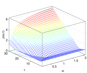
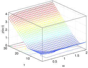
(a)	(b)

Figure 1: Surfaces of spectral radii of linear convolution operator $\mathcal{K}_{\text{\tiny$\triangle t$}}$ on finite time interval with respect to $\omega$ and $\tau$ based on BDF(1), $12\times 12$ grid and preconditioners (a) $Q_{1}$ and (b) $Q_{2}$.

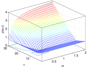
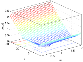
(a)	(b)

Figure 2: Surfaces of spectral radii of linear convolution operator $\mathcal{K}_{\text{\tiny$\triangle t$}}$ on finite time interval with respect to $\omega$ and $\tau$ based on BDF(2), $12\times 12$ grid and preconditioners (a) $Q_{1}$ and (b) $Q_{2}$.

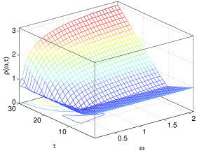
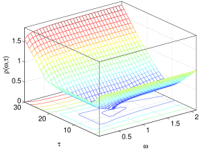
(a)	(b)

Figure 3: Surfaces of spectral radii of linear convolution operator $\mathcal{K}_{\text{\tiny$\triangle t$}}$ on finite time interval with respect to $\omega$ and $\tau$ based on BDF(3), $12\times 12$ grid and preconditioners (a) $Q_{1}$ and (b) $Q_{2}$.

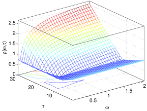
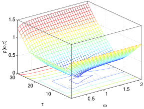
(a)	(b)

Figure 4: Surfaces of spectral radii of linear convolution operator $\mathcal{K}_{\text{\tiny$\triangle t$}}$ on finite time interval with respect to $\omega$ and $\tau$ based on BDF(4), $12\times 12$ grid and preconditioners (a) $Q_{1}$ and (b) $Q_{2}$.

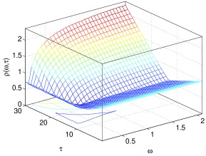
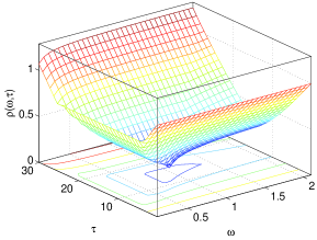
(a)	(b)

Figure 5: Surfaces of spectral radii of linear convolution operator $\mathcal{K}_{\text{\tiny$\triangle t$}}$ on finite time interval with respect to $\omega$ and $\tau$ based on BDF(5), $12\times 12$ grid and preconditioners (a) $Q_{1}$ and (b) $Q_{2}$.

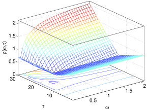
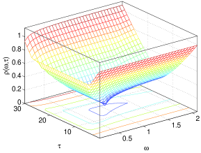
(a)	(b)

Figure 6: Surfaces of spectral radii of linear convolution operator $\mathcal{K}_{\text{\tiny$\triangle t$}}$ on finite time interval with respect to $\omega$ and $\tau$ based on BDF(6), $12\times 12$ grid and preconditioners (a) $Q_{1}$ and (b) $Q_{2}$.

6.2 Optimal Convergence Factor: Theoretical vs Practical

In Theorems 4.1 and 5.2, the general spectral radius formula of discrete-time waveform relaxation methods for solving general linear DAEs and the optimal convergence factor formula of the DABSOR method for solving linear DAEs derived from the time-dependent Stokes equations are discovered on finite time interval respectively. In this subsection, the comparison between theoretical and practical value of optimal convergence factor of the DABSOR method is exhibited. The computation of theoretical value is based on Theorems 4.1 and 5.2. The practical value represents the average experimental convergence rate.

The comparisons between theoretical and practical value of optimal convergence factor based on six different linear multistep formulae like BDF(1-6), two grid sizes as $12\times 12$, $24\times 24$ and two different choices of preconditioners $Q$ in Table 1 are presented in Tables 3-6. In these tables, DTOCF denotes the theoretical value of optimal convergence factor of the DABSOR method on finite time interval, APOCF represents the practical value of static iterative method for solving the system of linear equations with respect to coefficient matrix $\mathcal{A}$ in linear DAEs (1.6) and iterative matrix $\text{\bf K}(\sigma)$ with $\omega_{{\rm opt}}$ and $\tau_{{\rm opt}}$, and DPOCF($N$) is the practical value of optimal convergence factor of the DABSOR method with $N$ windows. After observing Tables 3-6, we find that the practical value DPOCF($N$) of the DABSOR method decreases when the the number of windows increases, and the larger the number of windows, the closer the practical value DPOCF($N$) to the theoretical value DTOCF. Specifically, for smaller number of windows, the computation load of the DABSOR method increases intensively because of larger spurious oscillations discussed in section 5.3 occurred on each window. Thus, the practical value DPOCF($N$) with small number of windows is far beyond the theoretical value DTOCF. When $N$ the number of windows increases, the spurious oscillations on each window becomes less apparent, and the DABSOR method tends to be more efficient. In addition, the practical value APOCF of the static iterative method is always smaller than the theoretical value DTOCF and practical value DPOCF($N$) of the DABSOR method, indicating that the convergence rate of the DABSOR method is unlikely to be faster than the corresponding static iterative method. On the other hand, theoretical and practical values based on preconditioner $Q_{2}$ are much smaller than that based on preconditioner $Q_{1}$, which means that preconditioner $Q_{2}$ always leads to faster convergence rate. The findings are consist with the results in subsection 6.1.

Table 3: Theoretical vs Practical: the optimal convergence factor based on $12\times 12$ grid and preconditioner $Q_{1}$

	BDF(1)	BDF(2)	BDF(3)	BDF(4)	BDF(5)	BDF(6)
DTOCF	0.3590	0.3921	0.4991	0.4812	0.5058	0.4943
APOCF	0.2154	0.2512	0.2154	0.2154	0.2154	0.2154
DPOCF(6)	0.7252	0.7834	0.8555	0.8918	0.9041	0.9056
DPOCF(12)	0.6519	0.6679	0.7960	0.8287	0.8417	0.8414
DPOCF(20)	0.6138	0.5695	0.7321	0.7687	0.7832	0.7803
DPOCF(30)	0.4527	0.4808	0.5985	0.5950	0.6152	0.6065
DPOCF(40)	0.3915	0.4206	0.5501	0.5424	0.5649	0.5530
DPOCF(60)	0.3237	0.3435	0.4855	0.4737	0.4946	0.4803

Table 4: Theoretical vs Practical: the optimal convergence factor based on $12\times 12$ grid and preconditioner $Q_{2}$

	BDF(1)	BDF(2)	BDF(3)	BDF(4)	BDF(5)	BDF(6)
DTOCF	0.2940	0.1804	0.0559	0.1098	0.1250	0.1084
APOCF	0.0631	0.0316	0.0316	0.0100	0.0316	0.0100
DPOCF(6)	0.6081	0.6302	0.6661	0.6585	0.7341	0.7282
DPOCF(12)	0.4892	0.4762	0.4728	0.4603	0.5754	0.5601
DPOCF(20)	0.4115	0.3490	0.3300	0.3051	0.4420	0.4215
DPOCF(30)	0.3516	0.2673	0.2053	0.2107	0.2457	0.2205
DPOCF(40)	0.3006	0.2083	0.1493	0.1590	0.1838	0.1520
DPOCF(60)	0.2379	0.1412	0.0926	0.0895	0.1176	0.0827

Table 5: Theoretical vs Practical: the optimal convergence factor based on $24\times 24$ grid and preconditioner $Q_{1}$

	BDF(1)	BDF(2)	BDF(3)	BDF(4)	BDF(5)	BDF(6)
DTOCF	0.3632	0.3298	0.5236	0.3408	0.5004	0.3493
APOCF	0.2154	0.2154	0.2154	0.2154	0.2154	0.2154
DPOCF(6)	0.6811	0.7525	0.8203	0.8188	0.8808	0.8567
DPOCF(12)	0.5875	0.6930	0.7603	0.7123	0.8061	0.7616
DPOCF(20)	0.5860	0.6271	0.6926	0.6156	0.7365	0.6722
DPOCF(30)	0.4684	0.4844	0.6039	0.4861	0.6026	0.4848
DPOCF(40)	0.4065	0.4189	0.5589	0.4168	0.5514	0.4158
DPOCF(60)	0.3412	0.3369	0.4973	0.3323	0.4816	0.3284

Table 6: Theoretical vs Practical: the optimal convergence factor based on $24\times 24$ grid and preconditioner $Q_{2}$

	BDF(1)	BDF(2)	BDF(3)	BDF(4)	BDF(5)	BDF(6)
DTOCF	0.4799	0.4061	0.3195	0.3097	0.2891	0.1871
APOCF	0.1000	0.0631	0.0631	0.0316	0.0316	0.0631
DPOCF(6)	0.5998	0.6641	0.6984	0.7475	0.7926	0.7880
DPOCF(12)	0.5231	0.5815	0.5894	0.6165	0.6703	0.6516
DPOCF(20)	0.5231	0.5149	0.4862	0.5044	0.5632	0.5326
DPOCF(30)	0.4282	0.4144	0.3569	0.3636	0.3537	0.3136
DPOCF(40)	0.3989	0.3649	0.2982	0.3021	0.2888	0.2398
DPOCF(60)	0.3506	0.3021	0.2267	0.2267	0.2107	0.1672

6.3 Accelerating Effect by Windowing Technique

In fact, the accelerating effect by windowing technique is revealed in the sense of practical optimal convergence factor in subsection 6.2. The larger the number of windows, the smaller the practical optimal convergence factor, or equivalently, the faster the convergence rate of the DABSOR method. In this subsection, the accelerating effect by windowing technique is exhibited in the sense of average number of iterative steps of the DABSOR method on each window.

The comparisons of average number of iterative steps of the DABSOR method based on six different linear multistep formulae like BDF(1-6), two grid sizes as $12\times 12$, $24\times 24$ and two different choices of preconditioners $Q$ in Table 1 are outlined in Tables 7-10. In these tables, NoW stands for the number of windows, NoU is the number of unknowns on each window, and “—” means the DABSOR method does not converge on at least one of the windows in 800 iterative steps. Obviously, the average number of iterative steps decreases in all kinds of situations when NoW increases, which implies a decrease to the computation load. In another word, the computation efficiency of the DABSOR method is greatly improved by applying windowing technique. Moreover, the average number of iterative steps of the DABSOR method based on preconditioner $Q_{2}$ is apparently smaller than that based on preconditioner $Q_{1}$, which tells the same story as in subsections 6.1 and 6.2.

It is known that high order time stepping schemes lead to high accuracy for solving ODEs and DAEs, meanwhile the computation load increases intensively. It is found in Tables 7-10 that the average number of iterative steps of the DABSOR method increases when the order of BDF becomes higher. For extreme situations, when NoW is small, the DABSOR methods based on high order BDF methods do not converge in 800 iterative steps. Hence, there should be a balance between computation accuracy and computation efficiency.

Table 7: Average number of iteration steps of the DABSOR method based on $12\times 12$ grid and preconditioner $Q_{1}$

NoW	BDF(1)	BDF(2)	BDF(3)	BDF(4)	BDF(5)	BDF(6)	NoU
1	161.0	412.0	—	—	—	—	51840
2	91.5	171.0	392.0	677.5	—	—	25920
3	68.0	112.7	233.0	369.0	472.7	691.7	17280
4	58.8	77.2	160.0	200.5	294.2	314.0	12960
5	48.8	64.8	118.8	147.0	201.0	211.8	10368
6	42.8	58.0	92.0	126.5	146.2	152.5	8640

Table 8: Average number of iteration steps of the DABSOR method based on $12\times 12$ grid and preconditioner $Q_{2}$

NoW	BDF(1)	BDF(2)	BDF(3)	BDF(4)	BDF(5)	BDF(6)	NoU
1	160.0	428.0	697.0	—	—	—	51840
2	76.0	134.0	210.5	373.5	717.5	—	25920
3	49.7	75.0	107.7	159.3	193.3	264.3	17280
4	36.8	47.5	71.2	87.5	121.2	125.2	12960
5	31.2	35.0	43.6	59.8	67.6	83.2	10368
6	27.7	30.7	35.3	34.7	47.7	47.7	8640

Table 9: Average number of iteration steps of the DABSOR method based on $24\times 24$ grid and preconditioner $Q_{1}$

NoW	BDF(1)	BDF(2)	BDF(3)	BDF(4)	BDF(5)	BDF(6)	NoU
1	154.0	350.0	721.0	—	—	—	207360
2	75.0	129.0	261.0	363.0	719.5	—	103680
3	54.7	80.7	162.0	176.3	283.3	379.0	69120
4	46.5	62.8	115.2	122.2	209.8	189.0	51840
5	39.0	53.8	87.8	91.6	148.4	129.6	41472
6	34.2	47.5	69.2	69.2	110.8	93.5	34560

Table 10: Average number of iteration steps of the DABSOR method based on $24\times 24$ grid and preconditioner $Q_{2}$

NoW	BDF(1)	BDF(2)	BDF(3)	BDF(4)	BDF(5)	BDF(6)	NoU
1	168.0	366.0	—	—	—	—	207360
2	76.0	138.5	238.0	325.5	601.0	—	103680
3	48.0	75.7	110.7	150.0	226.0	338.0	69120
4	35.0	47.5	68.2	98.0	118.8	153.8	51840
5	29.6	36.8	49.0	62.4	83.2	102.4	41472
6	25.7	33.0	38.2	47.5	60.5	60.7	34560

7 Concluding Remarks

This paper studies the general theory of the discrete-time waveform relaxation methods. Then, the DABSOR method is proposed for solving linear DAEs (1.6) derived from time-dependent Stokes equations (1.5). The convergence property and optimality of the DABSOR method are stated in detail. Due to the requirement of acceleration, the DABSOR method is integrated with windowing technique, which leads to great acceleration as shown in Section 6. In fact, further acceleration by algebraic techniques like Krylov subspace on each window is another path to improve the DABSOR method. The future work will follow right this path.

References

- [1] Z.-Z. Bai, B.N. Parlett and Z.-Q. Wang, On generalized successive overrelaxation methods for augmented linear systems, Numer. Math., 102(2005), 1-38.
- [2] Z.-Z. Bai, M.K. Ng and J.-Y. Pan, Alternating splitting waveform relaxation method and its successive overrelaxation acceleration, Comput. Math. Appl., 49(2005), 157-170.
- [3] Z.-Z. Bai and X. Yang, Continuous-time accelerated block successive overrelaxation methods for time-dependent Stokes equations, J. Comput. Appl. Math., 236(2012), 3265-3285.
- [4] Z.-Z. Bai and X. Yang, On convergence conditions of waveform relaxation methods for linear differential-algebraic equations, J. Comput. Appl. Math., 235(2011), 2790-2804.
- [5] K.E. Brenan, S.L. Campbell and L.R. Petzold, Numerical Solution of Initial-Value Problems in Differential-Algebraic Equations, North-Holland, New York and London, 1989.
- [6] G.H. Hardy, J.E. Littlewood and G. Pólya, Inequalities, 2nd ed., Cambridge University Press, Cambridge, 1978.
- [7] E. Hairer and G. Wanner, Solving Ordinary Differential Equations II: Stiff and Differential-Algebraic Problems, Springer-Verlag, Berlin and Heidelberg, 1996.
- [8] J. Janssen and S. Vandewalle, Multigrid waveform relaxation on spatial finite element methods: the discrete-time case, SIAM J. Sci. Comput., 17(1996), 133-155.
- [9] J. Janssen and S. Vandewalle, On SOR waveform relaxation methods, SIAM J. Numer. Anal., 34(1997), 2456-2481.
- [10] Y.-L. Jiang, A generel approach to waveform relaxation solutions of differetial-algebraic equations: the continuous-time and discrete-time cases, IEEE Trans. Circuits Systems I-Fundamental Theory and Appl., 51(2004), 1770-1780.
- [11] Y.-L. Jiang, Waveform Relaxation Methods, Science Press, Beijing, 2009.
- [12] Y.-L. Jiang and O. Wing, A note on the spectra and pseudospectra of waveform relaxation operators for linear differential-algebraic equations, SIAM J. Numer. Anal., 38(2000), 186-201.
- [13] C. Lubich, On the stability of linear multistep methods for Volterra convolution equations, IMA J. Numer. Anal., 3(1983), 439-465.
- [14] U. Miekkala, Dynamic iteration methods applied to linear DAE systems, J. Comput. Appl. Math., 25(1989), 133-151.
- [15] U. Miekkala and O. Nevanlinna, Sets of convergence and stability regions, BIT Numer. Math., 27(1987), 554-584.
- [16] U. Miekkala and O. Nevanlinna, Convergence of dynamic iteration methods for initial value problems, SIAM J. Sci. Stat. Comput., 8(1987), 459-482.
- [17] J.J.H. Miller, On the location of zeros of certain classes of polynomials with applications to numerical analysis, J. Inst. Math. Appl., 8 (1971) 397 C406.
- [18] O. Nevanlinna, Remarks on Picard-Lindelöf iteration, Part II, BIT Numer. Math., 29(1989), 535-562.
- [19] J.-Y. Pan and Z.-Z. Bai, On the convergence of waveform relaxation methods for linear initial value problems, J. Comput. Math., 22(2004), 681-698.
- [20] J.-Y. Pan, Z.-Z. Bai and M.K. Ng, Two-step waveform relaxation methods for implicit linear initial value problems, Numer. Linear Algebra Appl., 12(2005), 293-304.
- [21] J. Wang and Z.-Z. Bai, Convergence analysis of two-stage waveform relaxation method for the initial value problems, Appl. Math. Comput., 172(2006), 797-808.