Asymmetric Simple Exclusion Process with open boundaries and Quadratic Harnesses

Abstract.

We show that the joint probability generating function of the stationary measure of a finite state asymmetric exclusion process with open boundaries can be expressed in terms of joint moments of Markov processes called quadratic harnesses. We use our representation to prove the large deviations principle for the total number of particles in the system. We use the generator of the Markov process to show how explicit formulas for the average occupancy of a site arise for special choices of parameters. We also give similar representations for limits of stationary measures as the number of sites tends to infinity.

This is an expanded version with additional details that are omitted from the published version.

1. Introduction

1.1. Asymmetric simple exclusion process with open boundaries

Asymmetric simple exclusion process (ASEP) is a Markov model for random particles that cannot occupy the same position, and tend to move to the adjacent site with the rate that is larger to the right than to the left. There are several versions of the model; for example, Spitzer, [40] considers ASEP on the infinite number and on the finite number of sites. In this paper we are mostly interested in a particle system on a finite lattice of $N\geq 2$ points $S=\{1,\dots,N\}$, where each site $j\in S$ can have only $\tau_{j}=0$ or $\tau_{j}=1$ particles. The term “open boundary” refers to the fact that particles can be inserted and removed from both boundary points. This version of ASEP appeared in Liggett, [33, Section 3] and was extensively studied in physics, see e.g. [2, 5, 18, 19, 20, 21, 22]. A survey paper of Blythe and Evans, [6] gives additional references and motivation.

An informal description of the exclusion process is that particles are placed at rate $\alpha>0$ in position $1$, and at rate $\delta\geq 0$ in position $N$, provided the location is empty. Particles are also removed at rate $\gamma\geq 0$ from location $1$ and removed at rate $\beta>0$ from site $N$. Particles attempt to move to the nearest neighbor: to the right with rate 1 and to the left with rate $q\geq 0$; however they cannot move if the neighbor site is already occupied. Parameters $\alpha,\beta,\gamma,\delta$ describe behavior at the boundaries; parameter $q$ determines the degree of asymmetry, see Fig. 1. Exclusion process is symmetric, when $q=1$; the case $q>1$ is similar to $q<1$ due to “particles-holes duality”, see e.g. discussion of this point in [42]. Throughout this paper we will assume that $q<1$.

Figure 1. Asymmetric Simple Exclusion Process with open boundary and parameters $\alpha,\beta,\gamma,\delta,q$. Black disks represent occupied sites.

Time evolution of such a system is described by a continuous time Markov process $(\tau_{1}(t),\dots,\tau_{N}(t))$ with finite state space $\{0,1\}^{N}$, see e.g. [35, Formulas (2.1)-(2.3)]. We do not provide the details, as we are interested only in the (unique) invariant probability measure $\pi_{N}$ of the Markov chain $(\tau_{1}(t),\dots,\tau_{N}(t))$. Using the notation borrowed from statistical physics, by $\langle\cdot\rangle_{N}$ we denote the average with respect to this probability measure and by $(\tau_{1},\dots,\tau_{N})\in\{0,1\}^{N}$ we denote the random vector with the invariant distribution $\pi_{N}$. For example, $\langle\tau_{k}\rangle_{N}$ is the average occupancy of site $k$ with respect to $\pi_{N}$.

1.2. Overview of the main results

Our first main result, Theorem 1 in Section 2, relates joint probability generating function of $\tau_{1},\dots,\tau_{N}$ to the joint moments of a certain Markov processes $(Z_{t})_{t\geq 0}$, see (2.3). The Markov process comes from [12] where it is called a quadratic harness. It is described in more detail in Section 1.4. In Section 1.3, we review the matrix method of [20], which serves as an intermediate step in the proof of Theorem 1.

In Section 3, we use representation (2.3) to prove the large deviations principle for the total number of particles in the system. Theorem 7 extends the results of [23, Section 3.5] to the cases where particles can leave left boundary with rate $\gamma\neq 0$ and can be inserted at the right boundary with rate $\delta\neq 0$. The large deviations rate function depends on the parameters of the ASEP only through the support of random variable $Z_{t}$, see (3.9).

In Section 4 we give an integral formula for the average density profile when $\gamma=\delta=0$ and $\alpha+\beta>1-q$ and point out that the formula simplifies to a product form (4.17) when $q=0$. The proof of Theorem 9 uses the generator of the Markov process $(X_{t})$, which is given in Theorem 8.

In Section 5 we pass to the limit as the number of sites $N$ tends to infinity. The main result of this section, Theorem 13, represents the joint generating function of the limiting measure of the ASEP on the semi-infinite lattice in terms of the joint moments of a quadratic harness.

1.3. Matrix solution

The celebrated matrix method of Derrida et al., [20] introduces a probability measure on $\{0,1\}^{N}$ using a pair $\mathbf{D}$ and $\mathbf{E}$ of infinite matrices with $\mathbf{D}$ representing the occupied site, $\mathbf{E}$ representing an empty site, and a pair of vectors, where $\langle W|$ is a row vector and $|V\rangle$ is a column vector. It turns out that this is the invariant measure $\pi_{N}$ introduced in Section 1.1. For our purposes it is convenient to recast the expression from [20] into the formula for the joint generating function

(1.1) $$\left\langle\prod_{j=1}^{N}t_{j}^{\tau_{j}}\right\rangle_{N}=\frac{1}{K_{N}}\langle W|(\mathbf{E}+t_{1}\mathbf{D})(\mathbf{E}+t_{2}\mathbf{D})\dots(\mathbf{E}+t_{N}\mathbf{D})|V\rangle.$$

Here

(1.2) $$K_{N}=\langle W|(\mathbf{E}+\mathbf{D})^{N}|V\rangle$$

is the normalizing constant, which in the physics literature is called the partition function and is usually denoted by letter $Z$; in this paper, as in [12], we reserve letter $Z$ for a Markov process that we introduce in Section 1.4.

In ref. [20] the authors verify that $\langle\prod_{j=1}^{N}t_{j}^{\tau_{j}}\rangle_{N}$ is indeed the probability generating function of the invariant distribution $\pi_{N}$ of the exclusion process with parameters $\alpha,\beta,\gamma,\delta,q$, provided that the matrices and the vectors satisfy relations

(1.3) $$\mathbf{D}\mathbf{E}-q\mathbf{E}\mathbf{D} = \mathbf{D}+\mathbf{E},$$

(1.4) $$\langle W|(\alpha\mathbf{E}-\gamma\mathbf{D}) = \langle W|,$$

(1.5) $$(\beta\mathbf{D}-\delta\mathbf{E})|V\rangle = |V\rangle.$$

Derrida et al., [20] give a detailed proof for the case when $q=0$, and sketch the proof for the general $q$. Sandow, [35, Section III] proves the invariance of the probability measure determined by (1.1) for arbitrary $q$.

Formula (1.1) offers the flexibility of choosing convenient vectors and matrices. Refs. [20, 23, 25, 36, 42] show such choices for various ranges of the parameters, and use the explicit representations to derive properties of the ASEP. Our goal is to derive a representation for the left hand side of (1.1) in terms of moments of an auxiliary Markov process, called quadratic harness. We use this representation to study large deviations principle for the average occupation as well as mean values of occupation sites. In particular, we give simple derivations of some earlier known properties of ASEP.

Note that representation (1.1) cannot hold when $\langle W|V\rangle=0$, and Essler and Rittenberg, [26, page 1384] point out that this happens when $\alpha\beta=\gamma\delta$. They also point out the importance of a more general requirement $\alpha\beta-q^{k}\gamma\delta\neq 0$ for $k=0,1,\dots$. Our Markov process representation requires additional restrictions on the parameters, which in particular imply $\gamma\delta<\alpha\beta$.

1.4. Quadratic harnesses

In this section we introduce an auxiliary Markov processes, called quadratic harness, defined on another probability space which is unrelated to the probability space $(\{0,1\}^{N},\pi_{N})$ where the invariant measure $\pi_{N}$ is described through (1.1). To make the distinction more transparent, we denote by $\mathds{E}(X)$ the expected value of a random variable $X$ on this probability space. Our Markov process is different than the Markov process on permutation tableaux which was associated with ASEP in [16], and the way ASEP and the process we introduce are tied together is also different than the relation exhibited in [16]. However, there is a common thread of the Askey-Wilson polynomials in the background.

A square integrable (real) stochastic process $\mathbf{X}=(X_{t})_{t\in I}$ is called a quadratic harness on an interval $I$ if for $s<t<u$ we have

$$\mathds{E}(X_{t}|\mathcal{F}_{s,u})=\tfrac{u-t}{u-s}X_{s}+\tfrac{t-s}{u-s}X_{u},$$

and

$$\mathds{E}(X_{t}^{2}|\mathcal{F}_{s,u})=A_{tsu}X_{s}^{2}+B_{tsu}X_{s}X_{t}+C_{tsu}X_{u}^{2}+D_{tsu}X_{s}+E_{tsu}X_{u}+F_{tsu},$$

where $(\mathcal{F}_{s,u})_{s<u}$ is a past-future filtration of the process $\mathbf{X}$ and $A_{tsu},\ldots,F_{tsu}$ are non-random functions of $s,t,u$. We will say that $\mathbf{X}=(X_{t})_{t\in I}$ is a standard quadratic harness if $\mathds{E}\,X_{t}=0$, $\mathds{E}\,X_{s}X_{t}=s$, for $s<t$. It appears (see [8]) that under mild technical assumptions these conditions uniquely determine $\mathbf{X}$, which typically is a (non-homogeneous) Markov process. Moreover, the functions $A_{tsu},\ldots,F_{tsu}$ are defined in terms of five numerical constants $\theta,\eta\in\mathbb{R}$, $\tau,\sigma\geq 0$, $q_{0}\leq 1+2\sqrt{\tau\sigma}$ and, consequently,

$$\mathrm{Var}(X_{t}|\mathcal{F}_{s,u})=\tfrac{(u-t)(t-s)}{u(1+\sigma s)+\tau-\gamma s}K\left(\tfrac{X_{u}-X_{s}}{u-s},\tfrac{\tfrac{1}{s}X_{s}-\tfrac{1}{u}X_{u}}{\tfrac{1}{s}-\tfrac{1}{u}}\right)$$

with

$$K(x,y)=1+\theta x+\eta y+\tau x^{2}+\sigma y^{2}-(1-q_{0})xy.$$

That is, typically, a standard quadratic harness is determined by the constants $\theta,\eta,\tau,\sigma,q_{0}$, and thus we write $\mathbf{X}\sim\mathrm{QH}(\theta,\eta,\tau,\sigma,q_{0})$. The family of standard quadratic harnesses includes affine transformations of such processes as: Wiener process - $\mathrm{QH}(0,0,0,0,1)$, Poisson process - $\mathrm{QH}(\theta,0,0,0,1)$, $\theta>0$ and contains the whole class of Lévy-Meixner processes - $\mathrm{QH}(\theta,0,\tau,0,1)$ (see e.g. [38]). It contains also classical versions of free Brownian motion - $\mathrm{QH}(0,0,0,0,0)$ (see [4]), free Poisson process - $\mathrm{QH}(\theta,0,0,0,0)$ and the whole class of free Lévy-Meixner processes - $\mathrm{QH}(\theta,0,\tau,0,0)$ (see, e.g. [1]). Other examples of quadratic harnesses are quantum Bessel process - $\mathrm{QH}(\theta,\eta,0,0,1)$ (see [3], [10], or [34]), and a more general bi-Poisson process - $\mathrm{QH}(\theta,\eta,0,0,q)$ (see [9]), or the $q$-Brownian motion - $\mathrm{QH}(0,0,0,0,q)$ (see, e.g. [7]).

In Bryc and Wesołowski, [12] we use the orthogonality measures of Askey-Wilson polynomials to construct a large family of quadratic harnesses. We recall it with some details now since this approach will be used in order to connect quadratic harnesses with the ASEPs.

Let $q\in(-1,1)$ and $a,b,c,d\in\mathbb{C}$ be such that $abcd,abcdq,ab,abq\not\in[1,\infty)$. Following [12, (1.20)] we are interested in the family of Askey-Wilson polynomials defined through a three-term recurrence relation

(1.6) $$2x\bar{w}_{n}(x)=\bar{A}_{n}\bar{w}_{n+1}(x)+B_{n}\bar{w}_{n}(x)+\bar{C}_{n}\bar{w}_{n-1}(x),\qquad n\geq 0,$$

with $\bar{w}_{-1}\equiv 0$, $\bar{w}_{0}\equiv 1$ and

$$\bar{A}_{n}=\tfrac{(1-abcdq^{n-1})(1-abq^{n})}{(1-abcdq^{2n-1})(1-abcdq^{2n})},$$

$$B_{n}=a+\tfrac{1}{a}-\tfrac{(1-abcdq^{n-1})(1-abq^{n})(1-acq^{n})(1-adq^{n})}{a(1-abcdq^{2n-1})(1-abcdq^{2n})}\\ -a\tfrac{(1-q^{n})(1-bcq^{n-1})(1-bdq^{n-1})(1-cdq^{n-1})}{(1-abcdq^{2n-2})(1-abcdq^{2n-1})},$$

$$\bar{C}_{n}=\tfrac{(1-q^{n})(1-acq^{n-1})(1-adq^{n-1})(1-bcq^{n-1})(1-bdq^{n-1})(1-cdq^{n-1})}{(1-abcdq^{2n-2})(1-abcdq^{2n-1})}.$$

(The bars are solely for consistency with notation in [12].) When $\displaystyle\prod_{k=0}^{n}\bar{A}_{k}\bar{C}_{k+1}\geq 0$ for all $n$, the Askey-Wilson polynomials are orthogonal with respect to unique compactly supported probability measure $\nu(dx;a,b,c,d,q)$, which is called the Askey-Wilson distribution. It is not easy to describe in general for what choices of parameters $a,b,c,d,q$ such a measure exists. In Bryc and Wesołowski, [12, Lemma 3.1] sufficient conditions for existence were given in terms of two integers: $m_{1}=\#(\{ab,ac,ad,bc,bd,cd\}\cap[1,\infty))$ and $m_{2}=\#(\{abq,acq,adq,bcq,bdq,cdq\}\cap[1,\infty))$. For $a,b,c,d$ which are either real or come in complex conjugate pairs and such that $abcd<1$ and $abcdq<1$ the Askey-Wilson distribution exists in the following cases: (i) $q\geq 0$ and $m_{1}=0$; (ii) $q<0$ and $m_{1}=m_{2}=0$; (iii) $q\geq 0$, $m_{1}=2$; (iv) $q<0$, $m_{1}=2$, $m_{2}=0$; (v) $q<0$, $m_{1}=0$, $m_{2}=2$. In particular, in Section 5 we need to consider $ad=1$ and $ac>1$, which falls under case (iii), with degenerated measure $\nu$ concentrated at the root of $\bar{w}_{1}(x)$.

The Askey-Wilson measure has the form

$$\nu(dx;a,b,c,d,q)=f(x;a,b,c,d)I(|x|<1)dx+\sum_{y\in F(a,b,c,d,q)}\,p(y)\delta_{y}(dx),$$

where the density

(1.7) $$f(x;a,b,c,d,q)=\tfrac{(q,ab,ac,ad,bc,bd,cd)_{\infty}}{2\pi(abcd)_{\infty}\sqrt{1-x^{2}}}\,\left|\tfrac{\left(e^{2i\theta}\right)_{\infty}}{\left(ae^{i\theta},be^{i\theta},ce^{i\theta},de^{i\theta}\right)_{\infty}}\right|^{2},$$

with $\cos\,\theta=x$, may be sub-probabilistic or zero for some values of the parameters. The set $F=F(a,b,c,d,q)$ is a finite or empty set of atoms of $\nu(dx;a,b,c,d,q)$. If $\alpha\in\{a,b,c,d\}$ is such that $|\alpha|>1$ then $\alpha$ is real and generates atoms. E.g., if $|a|>1$ then it generates the atoms

(1.8) $$x_{j}=(aq^{j}+1/(aq^{j}))/2\mbox{ for $j=0,1,\dots$ such that $|aq^{j}|\geq 1$}$$

and the corresponding masses are

$$p(x_{0})=\tfrac{(a^{-2},bc,bd,cd)_{\infty}}{(b/a,c/a,d/a,abcd)_{\infty}},\;\\ p(x_{j})=p(x_{0})\tfrac{(a^{2},ab,ac,ad)_{j}\,(1-a^{2}q^{2j})}{(q,qa/b,qa/c,qa/d)_{j}(1-a^{2})}\,\left(\tfrac{q}{abcd}\right)^{j},\;j\geq 1.$$

In the formulas above, for complex $\alpha$ and $|q|<1$ we used $q$-Pochhammer symbol $(\alpha)_{n}:=(\alpha;q)_{n}=\prod_{j=0}^{n-1}\,(1-\alpha q^{j})$, $1\leq n\leq\infty$, $(\alpha)_{0}=1$. Moreover, $(a_{1},\ldots,a_{k})_{n}:=(a_{1})_{n}\ldots(a_{k})_{n}$, $0\leq n\leq\infty$.

We now use the Askey-Wilson measures $\nu(dx;a,b,c,d,q)$ to construct a Markov process which will depend on parameters $A,B,C,D,q$. As previously, we take $q\in(-1,1)$ and fix $A,B,C,D$ which are either real or $(A,B)$ or $(C,D)$ are complex conjugate pairs with $ABCD<1$, $qABCD<1$ and such that

(1.9) $$AC,AD,BC,BD,qAC,qAD,qBC,qBD\in\mathbb{C}\setminus[1,\infty).$$

The Askey-Wilson stochastic process $\mathbf{Y}=(Y_{t})_{t\in I}$, where

(1.10) $$I=\left[\max\{0,CD,qCD\},\,\tfrac{1}{\max\{0,AB,qAB\}}\right),$$

is defined as the Markov process with marginal distributions

(1.11) $$\pi_{t}(dx)=\nu(dx;A\sqrt{t},B\sqrt{t},C/\sqrt{t},D/\sqrt{t},q),\quad t\in I,$$

with compact support $U_{t}$, and the transition probabilities

(1.12) $$P_{s,t}(x,dy)=\nu(dy;A\sqrt{t},B\sqrt{t},\sqrt{s/t}(x+\sqrt{x^{2}-1}),\sqrt{s/t}(x-\sqrt{x^{2}-1})),\\ \quad s<t,\;s,t\in I,\;x\in U_{s}.$$

The marginal distribution $\pi_{t}(dx)$ may have atoms at points

(1.13) $$\frac{1}{2}\left(B\sqrt{t}q^{j}+\frac{1}{B\sqrt{t}q^{j}}\right),\;\frac{1}{2}\left(\frac{Dq^{j}}{\sqrt{t}}+\frac{\sqrt{t}}{Dq^{j}}\right),\;\\ \frac{1}{2}\left(A\sqrt{t}q^{j}+\frac{1}{A\sqrt{t}q^{j}}\right),\;\frac{1}{2}\left(\frac{Cq^{j}}{\sqrt{t}}+\frac{\sqrt{t}}{Cq^{j}}\right)\;.$$

These formulas are recalculated from (1.8) and appear explicitly in [12, (3.7) and (3.8)]. (Transition probabilities $P_{s,t}(x,dy)$ also may have atoms.)

To construct a standard quadratic harness from the Askey-Wilson process we introduced in [12, (2.22)] an intermediate (nonstandard) quadratic harness $\mathbf{Z}$ on $I$, which will be important for our further considerations in this paper. The process $\mathbf{Z}=(Z_{t})_{t\in I}$ is defined by

(1.14) $$Z_{t}=\tfrac{2\sqrt{t}}{\sqrt{1-q}}\,Y_{t},\mbox{$t\in I$}.$$

It is a Markov process with the following properties:

• $(Z_{t})$ has a sequence of orthogonal martingale polynomials

  $$\langle\mathbf{r}_{t}(x)|=[r_{0}(x;t),r_{1}(x;t),\dots],$$

  where

  (1.15) $$r_{n}(x;t)=t^{n/2}\bar{w}_{n}\left(\tfrac{\sqrt{1-q}}{2\sqrt{t}}x;A\sqrt{t},B\sqrt{t},C/\sqrt{t},D/\sqrt{t},q\right),\mbox{ $n=0,1,\dots$},$$

  with $\bar{w}_{n}(x)=\bar{w}_{n}(x;a,b,c,d,q)$ defined in (1.6). That is, $r_{n}(x;t)$ is a polynomial of degree $n$ in variable $x$ such that:

  1. $r_{0}(x;t)=1$;

  2. $\mathds{E}\left(r_{n}(Z_{t};t)r_{m}(Z_{t};t)\right)=0$ for $m\neq n$;

  3. $\mathds{E}(r_{n}(Z_{t};t)|Z_{s})=\mathds{E}(r_{n}(Z_{t};t)|\sigma(Z_{v}:v\leq s))=r_{n}(Z_{s};s)$ for $s\leq t$.

• The Jacobi matrix of the orthogonal polynomials $\{r_{n}(\cdot;t)\}$ is a tridiagonal infinite matrix which depends linearly on parameter $t$. We will write it as $t\mathbf{x}+\mathbf{y}$, and we will write the so called “three step recurrence” in vector notation as

  (1.16) $$x\langle\mathbf{r}_{t}(x)|=\langle\mathbf{r}_{t}(x)|(t\mathbf{x}+\mathbf{y}).$$

  This is recalculated from the recurrence (1.6), and appears in [12, page 1244].

• The Jacobi matrix is determined uniquely from the $q$-commutation equation

  (1.17) $$\mathbf{x}\mathbf{y}-q\mathbf{y}\mathbf{x}=\mathbf{I}$$

  and the initial conditions

  (1.18) $$\mathbf{x}=\left[\begin{matrix}\gamma_{0}&\varepsilon_{1}&0&\dots\\ \alpha_{0}&&&\\ 0&&&\\ \vdots&&&\\ \end{matrix}\right],\quad\mathbf{y}=\left[\begin{matrix}\delta_{0}&\varphi_{1}&0&\dots\\ \beta_{0}&&&\\ 0&&&\\ \vdots&&&\\ \end{matrix}\right]\,,$$

  where $\alpha_{0},\beta_{0},\gamma_{0},\delta_{0},\varepsilon_{1},\varphi_{1}$ depend on parameters $A,B,C,D,q$ through formulas in [12, page 1243]; these formulas are reproduced in the proof of Theorem 1 below, see e.g. (2.8).

Bryc and Wesołowski, [12] show that $(Z_{t})_{t\in I}$ is a Markov process with harness property

(1.19) $$\mathds{E}(Z_{t}|Z_{s},Z_{u})=\frac{u-t}{u-s}Z_{s}+\frac{t-s}{u-s}Z_{u}$$

and quadratic conditional variances under a two-sided conditioning. However, to obtain a standard quadratic harness an adjustment is necessary in order to fulfill the expectations and covariances requirements while preserving linearity of conditional expectations and quadratic form of conditional variances. This adjustment uses an invertible Möbius transformation $T(t)=\tfrac{t+CD}{1+ABt}$ and is of the form

(1.20) $$X_{t}=\tfrac{\sqrt{1-q}(1-ABt)Z_{T(t)}-(A+B)t-(C+D)}{\sqrt{(1-q)(1-AC)(1-AD)(1-BC)(1-BD)}}\,\sqrt{1-qABCD},\\ t\in J:=T^{-1}(I),$$

see [12, formula (2.28)].

Ref. [12, Theorem 1.1] states that $\mathbf{X}=(X_{t})_{t\in J}$ is a quadratic harness $\mathrm{QH}(\theta,\eta,\tau,\sigma,q_{0})$ with parameters

(1.21) $$\theta=-\tfrac{((C+D)(1+ABCD)-2CD(A+B))\sqrt{1-q}}{\sqrt{(1-AC)(1-AD)(1-BC)(1-BD)(1-qABCD)}},$$

(1.22) $$\eta=-\tfrac{((A+B)(1+ABCD)-2AB(C+D))\sqrt{1-q}}{\sqrt{(1-AC)(1-AD)(1-BC)(1-BD)(1-qABCD)}},$$

(1.23) $$\tau=\tfrac{CD(1-q)}{1-qABCD},\quad\sigma=\tfrac{AB(1-q)}{1-qABCD},\quad q_{0}=\tfrac{q-ABCD}{1-qABCD}.$$

Ref. [12, Theorem 1.2] assures that Markov process $(Z_{t})_{t\geq 0}$ exists when conditions (1.9) hold. In this paper we will only need real-valued parameters $A\geq 0,-1<B\leq 0,C\geq 0,-1<D\leq 0$, and $0\leq q<1$. Specialized to this case, (1.9) reduces to the condition $AC<1$.

2. Representing a matrix solution by the auxiliary Markov process

We now return to the study of invariant measure of ASEP with parameters $\alpha>0$, $\beta>0$, $\gamma\geq 0$, $\delta\geq 0$, $0\leq q<1$. Our goal is to associate an appropriate quadratic harness $(Z_{t})$ with the ASEP. Denote

(2.1) $$\kappa_{\pm}(u,v)=\frac{1-q-u+v\pm\sqrt{(1-q-u+v)^{2}+4uv}}{2u}\,.$$

Let $(Z_{t})_{t\geq 0}$ be the Markov process from (1.14) in Section 1.4 with parameters

(2.2) $$A=\kappa_{+}(\beta,\delta),\;B=\kappa_{-}(\beta,\delta),\;C=\kappa_{+}(\alpha,\gamma),\;D=\kappa_{-}(\alpha,\gamma).$$

Notice that $A,B,C,D$ are real, $ABCD=\gamma\delta/(\alpha\beta)$, and $A,C\geq 0$ while $-1<B,D\leq 0$. Indeed, it is clear that $\kappa_{-}(u,v)\leq 0$ when $u>0$, $v\geq 0$. Inequality $\kappa_{-}(u,v)>-1$ is equivalent to $1-q+u+v>\sqrt{(1-q-u+v)^{2}+4uv}$. Since $q<1$ and $u,v\geq 0$, the left hand side is positive. Upon squaring both sides we see that $\kappa_{-}(u,v)>-1$ is equivalent to $4u(1-q)>0$.

In particular, $BD<1$, so $(Z_{t})_{t\in I}$ is well defined when $AC<1$ and from (1.10) we get $I=(0,\infty)$.

Our main result is the following representation of the joint generating function of the invariant measure of the ASEP in terms of the stochastic process $(Z_{t})$.

Theorem 1.

Suppose that the parameters of ASEP are such that $AC<1$. Then for $0<t_{1}\leq t_{2}\leq\dots\leq t_{N}$ the joint generating function of the invariant measure of the ASEP is

(2.3) $$\left\langle\prod_{j=1}^{N}t_{j}^{\tau_{j}}\right\rangle_{N}=\frac{\mathds{E}\left(\prod_{j=1}^{N}(1+t_{j}+\sqrt{1-q}\,Z_{t_{j}})\right)}{\mathds{E}\left((2+\sqrt{1-q}\,Z_{1})^{N}\right)}.$$

Since the left hand side is a polynomial in $t_{1},\dots,t_{N}$, it is clear that formula (2.3) determines $\langle\prod_{j=1}^{N}t_{j}^{\tau_{j}}\rangle_{N}$ uniquely for all $t_{1},\dots,t_{N}$.

The proof of Theorem 1 appears in Section 2.1. We conclude this section with remarks.

Remark 2.

Assumption $AC<1$ has natural physical interpretation – in terminology of [23] it identifies the “fan region” of ASEP. Since $0\leq BD<1$, we have

$$\frac{\gamma\delta}{\alpha\beta}=ABCD<1,$$

so the conditions [26, (58)] for the existence of a matrix representation are automatically satisfied.

Remark 3.

Suppose that $(Z_{t})$ is a Markov process from Section 1.4 with $0\leq q<1$ and with parameters $A,B,C,D$ which satisfy (1.9). If in addition  $A,B,C,D$ are real, $q\geq 0$, $(1+A)(1+B)>0$, $(1+C)(1+D)>0$, and $AB\leq 0$, $CD\leq 0$, then the right hand side of (2.3) determines the invariant measure of an ASEP with parameters

(2.4) $$\alpha=\frac{1-q}{(1+C)(1+D)},\;\beta=\frac{1-q}{(1+A)(1+B)},\;\gamma=\frac{-(1-q)CD}{(1+C)(1+D)},\\ \delta=\frac{-(1-q)AB}{(1+A)(1+B)}.$$

Remark 4.

A special case of formula (2.3) relates $\langle t^{\sum_{j=1}^{n}\tau_{j}}\rangle_{N}$ to the $N$-th moment of $(1+t+\sqrt{1-q}Z_{t})$, i.e., to the moments of an Askey-Wilson law. Therefore exact formula for $\mathds{E}\left((2+\sqrt{1-q}Z_{1})^{N}\right)/(1-q)^{N}$ when $\gamma=\delta=0$ can be read from [5, Equation (57)]. Josuat-Vergès, 2011a [30, Theorem 1.3.1] and [31, Theorem 6.1] used combinatorial techniques to generalize this to the exact formula for $\mathds{E}\left((1+t+\sqrt{1-q}Z_{t})^{N}\right)/(1-q)^{N}$. For a more analytic approach, see [41]. Formulas for moments of more general Askey-Wilson laws appear in [15, 32].

Remark 5.

The right hand side of (2.3) may define a probability generating function of a probability measure for other values of parameters than those specified in the assumptions of Theorem 1. In Theorem 13 we show that a semi-infinite ASEP is related to (2.3) with parameters that do not correspond to an ASEP. Johnston and Stringer, [29] consider another “non-physical” case $q=-1$.

2.1. Proof of Theorem 1

Our motivation and starting point is Ref. [42] which represents matrices $\mathbf{E},\mathbf{D}$ by the Jacobi matrices of the Askey-Wilson polynomials, with vectors $\langle W|=[1,0,0,\dots]$ and $|V\rangle=[1,0,0,\dots]^{T}$. Ref. [42] then uses these matrices to give the integral formulae for the partition function and for the $m$-point correlation function $\langle\tau_{j_{1}}\tau_{j_{2}}\dots\tau_{j_{m}}\rangle$. These integral formulas inspired our search for representation in terms of the quadratic harnesses.

We begin with a slight variation of [42, formula (4.5)]. We use matrices $\mathbf{x}$, $\mathbf{y}$ from (1.16) to rewrite $\mathbf{E},\mathbf{D}$ as

(2.5) $$\mathbf{E}=\frac{1}{1-q}\mathbf{I}+\frac{1}{\sqrt{1-q}}\,\mathbf{y},\quad\mathbf{D}=\frac{1}{1-q}\mathbf{I}+\frac{1}{\sqrt{1-q}}\,\mathbf{x}\,,$$

compare [5, formulas (13) and (14)]. (This is simply a rescaling by the factor $1/\sqrt{1-q}$ of the two operators in [42, formula (4.5)].) Then, just like in [42], formulas (1.17) and (1.3) are equivalent.

Next, we use (1.18) to ensure that (1.5) and (1.4) hold with vectors $\langle W|=[1,0,0,\dots]$ and $|V\rangle=[1,0,0,\dots]^{T}$. In order for (1.5) to hold, in (1.18) we must have

(2.6) $$\beta\alpha_{0}-\delta\beta_{0}=0$$

and

(2.7) $$\frac{\beta-\delta}{1-q}+\frac{\beta\gamma_{0}-\delta\delta_{0}}{\sqrt{1-q}}=1.$$

Since according to [12, page 1243], $\alpha_{0}=-AB\beta_{0}$, equation (2.6) gives $AB=-\delta/\beta$. The expressions for $\gamma_{n}$ and $\delta_{n}$ presented in [12, page 1243] for $n=0$ give

(2.8) $$\gamma_{0}=\frac{A+B-AB(C+D)}{\sqrt{1-q}(1-ABCD)},\;\delta_{0}=\frac{C+D-CD(A+B)}{\sqrt{1-q}(1-ABCD)}.$$

We note that condition $ABCD<1$ implies that $\alpha\beta-\gamma\delta\neq 0$, so inserting these expressions into (2.7), we get $(1+C+D)\alpha=1-q+\gamma$.

Similarly, in order for (1.4) to hold, we must have $\alpha\varphi_{1}-\gamma\varepsilon_{1}=0$, which in view of relation $\varphi_{1}=-CD\varepsilon_{1}$ [12, page 1243] gives $CD=-\gamma/\alpha$. Finally, we need to ensure that

$$\frac{\alpha-\gamma}{1-q}+\frac{\alpha\delta_{0}-\gamma\gamma_{0}}{\sqrt{1-q}}=1.$$

Using (2.8) and $\alpha\beta\neq\gamma\delta$, this simplifies to $(1+A+B)\beta=1-q+\delta$. The system of four equations for $A,B,C,D$ decouples, and we get a pair of one-variable quadratic equations for the unknowns $A,C$, with solutions (2.2).

We now choose $t_{1}\leq t_{2}\leq\dots\leq t_{N}$ and, after including the factor $(1-q)^{N}$ into the normalizing constant, we rewrite the unnormalized matrix expression on the right hand side of (1.1) as

(2.9) $$\langle W|\mathop{\stackrel{{\scriptstyle\to}}{{\prod}}}_{j=1}^{N}(\mathbf{E}+t_{j}\mathbf{D})|V\rangle\\ =\frac{1}{(1-q)^{N}}\langle W|\mathop{\stackrel{{\scriptstyle\to}}{{\prod}}}_{j=1}^{N}((1+t_{j})\mathbf{I}+\sqrt{1-q}(t_{j}\mathbf{x}+\mathbf{y}))|V\rangle:=\frac{1}{(1-q)^{N}}\Pi.$$

Since polynomials $\{r_{n}(x;t)\}$ are orthogonal and $r_{0}(x;t)=1$, we have $\langle W|=\mathds{E}(\langle\mathbf{r}_{t_{1}}(Z_{t_{1}})|)$ which gives

$$\Pi=\mathds{E}\left(\Big{\langle}\mathbf{r}_{t_{1}}(Z_{t_{1}})\Big{|}\mathop{\stackrel{{\scriptstyle\to}}{{\prod}}}_{j=1}^{N}((1+t_{j})\mathbf{I}+\sqrt{1-q}(t_{j}\mathbf{x}+\mathbf{y}))\big{|}V\Big{\rangle}\right).$$

By (1.16),

$$\big{\langle}\mathbf{r}_{t}(Z_{t})\big{|}\left((1+t)\mathbf{I}+\sqrt{1-q}(t\mathbf{x}+\mathbf{y})\right)=(1+t+\sqrt{1-q}Z_{t})\big{\langle}\mathbf{r}_{t}(Z_{t})\big{|},$$

so

$$\Pi=\mathds{E}\Big{(}\left(1+t_{1}+\sqrt{1-q}Z_{t_{1}}\right)\\ \times\big{\langle}\mathbf{r}_{t_{1}}(Z_{t_{1}})\big{|}\mathop{\stackrel{{\scriptstyle\to}}{{\prod}}}_{j=2}^{N}((1+t_{j})\mathbf{I}+\sqrt{1-q}(t_{j}\mathbf{x}+\mathbf{y}))\big{|}V\big{\rangle}\Big{)}.$$

We now use this formula, martingale property of $\{r_{n}(Z_{t};t)\}$ and standard properties of conditional expectations. We get

$$\Pi=\mathds{E}\Big{(}(1+t_{1}+\sqrt{1-q}Z_{t_{1}})\\ \times\mathds{E}(\langle\mathbf{r}_{t_{2}}(Z_{t_{2}})|\mathop{\stackrel{{\scriptstyle\to}}{{\prod}}}_{j=2}^{N}((1+t_{j})\mathbf{I}+\sqrt{1-q}(t_{j}\mathbf{x}+\mathbf{y}))|V\rangle|Z_{t_{1}})\Big{)}\\ =\mathds{E}\Big{(}(1+t_{1}+\sqrt{1-q}Z_{t_{1}})\\ \times\langle\mathbf{r}_{t_{2}}(Z_{t_{2}})|\mathop{\stackrel{{\scriptstyle\to}}{{\prod}}}_{j=2}^{N}((1+t_{j})\mathbf{I}+\sqrt{1-q}(t_{j}\mathbf{x}+\mathbf{y}))|V\rangle\Big{)}\\ =\mathds{E}\Big{(}\prod_{i=1}^{2}(1+t_{i}+\sqrt{1-q}Z_{t_{i}})\langle\mathbf{r}_{t_{2}}(Z_{t_{2}})|\mathop{\stackrel{{\scriptstyle\to}}{{\prod}}}_{j=3}^{N}((1+t_{j})\mathbf{I}+\sqrt{1-q}(t_{j}\mathbf{x}+\mathbf{y}))|V\rangle\Big{)}\\ =\mathds{E}\Big{(}\prod_{i=1}^{2}(1+t_{i}+\sqrt{1-q}Z_{t_{i}})\\ \times\mathds{E}\Big{(}\big{\langle}\mathbf{r}_{t_{3}}(Z_{t_{3}})\big{|}\mathop{\stackrel{{\scriptstyle\to}}{{\prod}}}_{j=3}^{N}((1+t_{j})\mathbf{I}+\sqrt{1-q}(t_{j}\mathbf{x}+\mathbf{y}))\big{|}V\big{\rangle}\Big{|}Z_{t_{1}},Z_{t_{2}}\Big{)}\Big{)}.$$

Recurrently, we get

(2.10) $$\Pi=\mathds{E}\left(\prod_{i=1}^{N}(1+t_{i}+\sqrt{1-q}Z_{t_{i}})\langle\mathbf{r}_{t_{N}}(Z_{t_{N}})|V\rangle\right).$$

Recall now that $r_{0}(x;t)=1$ and $|V\rangle=[1,0,0,\dots]^{T}$, so $\langle\mathbf{r}_{t_{N}}(Z_{t_{N}})|V\rangle=r_{0}(Z_{t_{N}};t_{N})=1$. Thus (2.9) and (2.10) give

$$\big{\langle}W\big{|}\mathop{\stackrel{{\scriptstyle\to}}{{\prod}}}_{j=1}^{N}(\mathbf{E}+t_{j}\mathbf{D})\big{|}V\big{\rangle}=\frac{1}{(1-q)^{N}}\mathds{E}\left(\prod_{j=1}^{N}\left(1+t_{j}+\sqrt{1-q}Z_{t_{j}}\right)\right).$$

By (1.1), this proves (2.3).

Remark 6.

The normalizing constant $K_{N}$ from (1.2) enters many exact formulas in the literature. Of course, the (new) normalizing constant is just the value of the expression $\mathds{E}\left(\prod_{j=1}^{N}\left(1+t_{j}+\sqrt{1-q}Z_{t_{j}}\right)\right)$ at $t_{j}=1$. Our proof used matrix representation (1.1) with $\langle W|V\rangle=1$; by homogeneity, in general the new normalization is related to $K_{N}$ by formula

(2.11) $$\mathds{E}\left((2+\sqrt{1-q}\,Z_{1})^{N}\right)=\frac{(1-q)^{N}}{\langle W|V\rangle}K_{N}.$$

3. Application to large deviations

This section shows how one can use representation (2.3) to prove the large deviations principle for $\tfrac{1}{N}\sum_{j=1}^{N}\tau_{j}$.

For $q=0$, $\alpha,\beta>1$ and $\gamma=\delta=0$ this result was announced in [21, (30)]. LDP for general $q$ appears in [23, Section 3.5], as an application to a more general path-level LDP. The general case with $\gamma,\delta\geq 0$ is described in the introduction to [25], but it seems that no proof is available in the literature: in [23] the authors write only: the calculations in the case of nonzero $\gamma$ or $\delta$ are more complicated, and for that reason we limit our analysis in the present paper to the case $\gamma=\delta=0$. Our proof is a good illustration of the use of Theorem 1 to get rigorous proofs when the parameters of the ASEP are within its range of applicability.

For an ASEP with parameters $\alpha,\beta,\gamma,\delta,q$, define $A,B,C,D$ by (2.2) and let

(3.1) $$\rho_{0} = \frac{1}{1+C}=\frac{1-q+\alpha+\gamma-\sqrt{(1-q-\alpha+\gamma)^{2}+4\alpha\gamma}}{2(1-q)},$$

(3.2) $$\rho_{1} = \frac{A}{1+A}=\frac{1-q-\beta-\delta+\sqrt{(1-q-\beta+\delta)^{2}+4\beta\delta}}{2(1-q)}.$$

(These are [25, (1.1a) and (1.1b)] and [26, formula (100)].) Assumption $AC<1$ is equivalent to $\rho_{0}>\rho_{1}$, and this is the only case that we analyze here.

Next, we define

(3.3) $$\mbox{L}_{0}=-\sup_{\rho_{1}\leq\rho\leq\rho_{0}}\log(\rho(1-\rho))\\ =\begin{cases}-\log(\rho_{0}(1-\rho_{0}))=2\log(\sqrt{C}+\frac{1}{\sqrt{C}})&\mbox{if $C>1$, i.e., $\rho_{0}<1/2$},\\ -\log(\rho_{1}(1-\rho_{1}))=2\log(\sqrt{A}+\frac{1}{\sqrt{A}})&\mbox{if $A>1$, i.e., $\rho_{1}>1/2$},\\ \log 4&\mbox{if $A,C<1$, i.e., $\tfrac{1}{2}\in[\rho_{1},\rho_{0}]$}.\\ \end{cases}$$

compare [23, expression (1.5)] or [25, expression (1.7)]. The rate function depends on the relative entropy of Bernoulli distributions:

(3.4) $$h(x|p)=x\log\tfrac{x}{p}+(1-x)\log\tfrac{1-x}{1-p}\mbox{ for $x\in[0,1],p\in(0,1)$}.$$

Theorem 7.

Suppose that the parameters of ASEP are such that $\rho_{0}>\rho_{1}$. Then the sequence $\{\bar{\tau}_{N}:=\frac{1}{N}\sum_{j=1}^{N}\tau_{j}\}_{N\in\mathds{N}}$ satisfies the large deviations principle with speed $N$ and the rate function

(3.5) $$\mbox{I}(x)=\begin{cases}h(x|\rho_{0})+\mbox{L}_{0}+\log(\rho_{0}(1-\rho_{0}))&\mbox{if $0\leq x<1-\rho_{0}$},\\ 2h(x|\tfrac{1}{2})+\mbox{L}_{0}-\log 4&\mbox{if $1-\rho_{0}\leq x\leq 1-\rho_{1}$},\\ h(x|\rho_{1})+\mbox{L}_{0}+\log(\rho_{1}(1-\rho_{1}))&\mbox{if $1-\rho_{1}<x\leq 1$},\\ \infty&\mbox{ if $x<0$ or $x>1$}.\end{cases}$$

That is, denoting by $\pi_{N}$ the invariant measure on $\{0,1\}^{N}$ with generating function (1.1), we have

(3.6) $$\lim_{N\to\infty}\frac{1}{N}\log\pi_{N}(\bar{\tau}_{N}\in(a,b))=-\inf_{x\in(a,b)}\mbox{I}(x)$$

for any $0\leq a<b\leq 1$.

Recall that $\pi_{N}(\bar{\tau}_{N}\in(a,b))$ is an abbreviation for $\pi_{N}(\{\tau\in\{0,1\}^{N}:\,\bar{\tau}_{N}\in(a,b)\})$. We remark that since the rate function $\mbox{I}(\cdot)$ is continuous on $[0,1]$, the upper/lower bounds of the “standard statement” of the large deviations principle coincide on the subintervals of $[0,1]$.

Theorem 7 formally extends [23, Section 3.5, formula (3.12)] to allow (some) $\gamma,\delta$. It also includes the LDP announced in [21, formula (30)], who considered the case $\alpha,\beta>1$ and $\gamma=\delta=q=0$. Indeed, if $\gamma=\delta=0$ and $\alpha>1-q$, $\beta>1-q$ then (2.1) and (2.2) give $A=C=0$. So $\rho_{0}=1$, $\rho_{1}=0$ and the rate function is $I(x)=2h(x|1/2)$ for $0\leq x\leq 1$.

In particular, Theorem 7 recovers part of the “phase diagram” [18, 20, 25, 39]: from (3.5) and (3.3) it is easy to locate the unique zero of $\mbox{I}(x)$, so that $\bar{\tau}_{N}$ converges exponentially fast to either $\rho_{0}$, if $\rho_{0}<1/2$ (the so called low density phase), to $\rho_{1}$, if $\rho_{1}>1/2$ (the so called high density phase), or to $1/2$, if $1/2\in[\rho_{1},\rho_{0}]$ (the so called maximal current phase).

Proof.

The proof is based on a routine application of the Laplace transform method from the Gärtner-Ellis Theorem [17, Theorem 2.3.6]. That is, we compute the limit

(3.7) $$\Lambda(\lambda)=\lim_{N\to\infty}\frac{1}{N}\log\langle\exp(N\lambda\bar{\tau}_{N})\rangle_{N}=\lim_{N\to\infty}\frac{1}{N}\log\left\langle\exp(\lambda\sum_{j=1}^{N}\tau_{j})\right\rangle_{N}$$

for real $\lambda$. In view of (2.3), this amounts to calculation of the limit

(3.8) $$\mbox{L}(\lambda)=\lim_{N\to\infty}\frac{1}{N}\log\mathds{E}\left((1+e^{\lambda}+\sqrt{1-q}Z_{e^{\lambda}})^{N}\right),$$

with $\Lambda(\lambda)=\mbox{L}(\lambda)-\mbox{L}(0)$.

Our goal is to show that $1+e^{\lambda}+\sqrt{1-q}Z_{e^{\lambda}}\geq 0$, so

(3.9) $$\mbox{L}(\lambda)=\log\|1+e^{\lambda}+\sqrt{1-q}Z_{e^{\lambda}}\|_{\infty}$$

depends only on the support of the single random variable $Z_{t}$, and is given by explicit formula (3.12) below.

We determine the support of $\sqrt{1-q}Z_{t}$ from the support of a closely related random variable $Y_{t}$ in [12, (2.22)]. From [12, Section 3.2], we read out that the distribution of $Z_{t}$ has only absolutely continuous and discrete parts. The absolutely continuous part of the law of $\sqrt{1-q}Z_{t}$ is supported on the interval $[-2\sqrt{t},2\sqrt{t}]$, because the continuous part of $Y_{t}$ is supported on $[-1,1]$. The locations of atoms of $\sqrt{1-q}Z_{t}$ are calculated from (1.13) and (1.8). Recalling that according to (2.2), we have $A,C\geq 0$ and $B,D\leq 0$, the atoms appear above (i.e., to the right of) the support $[-2\sqrt{t},2\sqrt{t}]$ of the continuous part at points

$$Atq^{j}+\frac{1}{Aq^{j}}\mbox{ for $t>\frac{1}{A^{2}q^{2j}}$},\;Cq^{j}+\frac{t}{Cq^{j}}\mbox{ for $t<C^{2}q^{2j}$},$$

and they appear below (i.e., to the left of) the support $[-2\sqrt{t},2\sqrt{t}]$ of the continuous part at points

$$Btq^{j}+\frac{1}{Bq^{j}}\mbox{ for $t>\frac{1}{B^{2}q^{2j}}$},\;Dq^{j}+\frac{t}{Dq^{j}}\mbox{ for $t<D^{2}q^{2j}$}.$$

The atoms above the support of the continuous part lie below the pair of the atoms that correspond to $j=0$, and there are no atoms above the support of the continuous part when $C^{2}<t<1/A^{2}$ (recall that this interval is nonempty by assumption (2.2)). Similarly, the atoms below the support of the continuous part lie above the pair of the atoms that correspond to $j=0$. So the support of $\sqrt{1-q}Z_{t}$ is contained between the pair of continuous curves. The upper boundary is

(3.10) $$U(t)=\begin{cases}C+t/C&\mbox{if $t\leq C^{2}$},\\ 2\sqrt{t}&\mbox{if $C^{2}<t<1/A^{2}$},\\ At+1/A&\mbox{if $t\geq 1/A^{2}$},\end{cases}$$

and the lower boundary is

(3.11) $$\ell(t)=\begin{cases}D+t/D&\mbox{ if $t\leq D^{2}$},\\ -2\sqrt{t}&\mbox{ if $D^{2}<t<1/B^{2}$},\\ Bt+1/B&\mbox{ if $t\geq 1/B^{2}$}\,.\end{cases}$$

The boundaries do not depend on the value of parameter $0\leq q<1$. Fig. 2 illustrates how the support of $Z_{t}$ varies with $t$ for $q=0$.

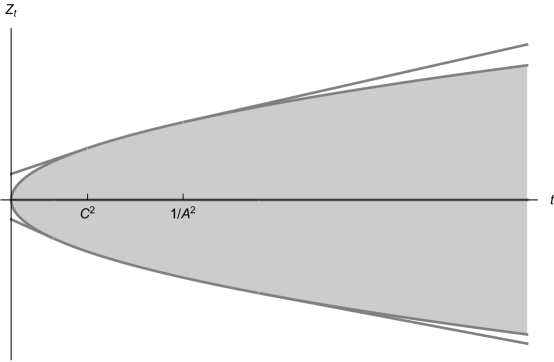
Figure 2. Support of $Z_{t}$ for $q=0$, $A,C>0$, $B,D<0$. The shaded gray area between the parabolas represents the support $[-2\sqrt{t},2\sqrt{t}]$ of the continuous part of the distribution. The four tangent gray lines represent the locations of the atoms for $t>0$.

To verify that $1+t+\sqrt{1-q}Z_{t}\geq 0$, we inspect each of the cases and verify that $1+t+\ell(t)\geq(1-\sqrt{t})^{2}\geq 0$:

1. for $t\leq D^{2}$ with negative $D$, we have $1+t+D+t/D=(D+t)(1+1/D)\geq(1-\sqrt{t})^{2}$ as $D\mapsto D+t/D$ with derivative $1-t/D^{2}\geq 0$ is increasing on $-\sqrt{t}<D<0$;

2. for any $t$, $1+t-2\sqrt{t}=(1-\sqrt{t})^{2}\geq 0$;

3. for $t\geq 1/B^{2}$ with negative $B$, we have $1+t+tB+1/B=(B+1)(t+1/B)\geq(1-\sqrt{t})^{2}$, as $B\mapsto tB+1/B$ with derivative $t-1/B^{2}\geq 0$ is increasing on $-1/\sqrt{t}<B<0$.

Since we proved that $1+t+\sqrt{1-q}Z_{t}\geq 0$, we can now insert the absolute value and the limit (3.8) becomes just the logarithm of the infinity norm $\|1+e^{\lambda}+\sqrt{1-q}Z_{e^{\lambda}}\|_{\infty}$. The explicit value of the limit can now be read out from (3.10). We get

(3.12) $$\mbox{L}(\lambda)=\begin{cases}\log(C+e^{\lambda})+\log\frac{1+C}{C}&\mbox{if $e^{\lambda}<C^{2}$},\\ 2\log(1+e^{\lambda/2})&\mbox{ if $C^{2}<e^{\lambda}<1/A^{2}$},\\ \log(1+Ae^{\lambda})+\log\frac{1+A}{A}&\mbox{ if $e^{\lambda}>1/A^{2}$}.\end{cases}$$

Accounting for the normalization which is needed in (3.7), we get $\Lambda(\lambda)=\mbox{L}(\lambda)-\mbox{L}(0)$. A calculation confirms that $\mbox{L}_{0}:=\mbox{L}(0)$ is indeed given by (3.3).

Since the function $\lambda\mapsto\Lambda(\lambda)$ is differentiable at all $\lambda$, the LDP follows with

$$\mbox{I}(x)=\sup_{\lambda}\{\lambda x-\Lambda(\lambda)\}=\mbox{L}_{0}+\sup_{\lambda}\{\lambda x-\mbox{L}(\lambda)\}.$$

To derive the three explicit expressions given in (3.5) we note that

$$\mbox{L}^{\prime}(\lambda)=\begin{cases}\frac{e^{\lambda}}{C+e^{\lambda}}&\mbox{with $e^{\lambda}<C^{2}$ has range $(0,C/(1+C))$ },\\ \frac{e^{\lambda/2}}{1+e^{\lambda/2}}&\mbox{with $C^{2}\leq e^{\lambda}\leq 1/A^{2}$ has range $[C/(1+C),1/(1+A)]$ },\\ \frac{Ae^{\lambda}}{1+Ae^{\lambda}}&\mbox{with $e^{\lambda}>1/A^{2}$ has range $(1/(1+A),1)$}.\end{cases}$$

After a calculation, this gives each of the cases listed in (3.5) for $x\in(0,1)$. The value for $\mbox{I}(x)$ with $x\leq 0$ arises from $\lambda\to-\infty$ with $\mbox{L}(\lambda)\to\log(1+C)$. The value for $\mbox{I}(x)$ with $x\geq 1$ arises from taking $\lambda\to\infty$ with $\lambda x-\mbox{L}(\lambda)=(x-1)\lambda+(\lambda-\mbox{L}(\lambda))$ and noting that $\lambda-\mbox{L}(\lambda)=\log\frac{e^{\lambda}}{1+Ae^{\lambda}}-\log\frac{1+A}{A}\to-\log(1+A)$ is bounded. (The above is a routine entropy calculation that we included for completeness.)

∎

4. Some explicit formulas

Some “miraculous” explicit formulas for the average occupation $\langle\tau_{k}\rangle_{N}$ of site $k$ for a system of length $N$ appear in [18, Formulas (47) and (48)] in the case $q=0$, $\alpha=\beta=1$, $\gamma=\delta=0$. The first of them is generalized to arbitrary $\alpha,\beta$ in [20, expressions (39) and (43)] and in [39]. In particular, Schütz and Domany, [39, formula (3.3)] point out a factorization of the expression for the difference $\langle\tau_{k}\rangle_{N}-\langle\tau_{k+1}\rangle_{N}$ and discuss several implications of the factorization.

Our goal in this section is to explore Theorem 1 to gain quick access to some of such explicit formulas.

4.1. Integral formulas for $K_{N}$

Of course, (2.11) is an integral formula for $K_{N}$, expressing $K_{N}$ as a constant times the integral of $(2+\sqrt{1-q}x)^{N}$ with respect to the law of $Z_{1}$. This is essentially [42, expression (6.1)] or [43, expression (3.12)]. When $-1<A,B,C,D<1$, the law is absolutely continuous with the Askey-Wilson density (1.7), which in general involves infinite products. For $q=0$, the infinite products vanish and the density takes a more concise form. We get

(4.1) $$K_{N}=M\int_{-2}^{2}\frac{(2+x)^{N}\sqrt{4-x^{2}}}{(1+A^{2}-Ax)(1+B^{2}-Bx)(1+C^{2}-Cx)(1+D^{2}-Dx)}dx\,,$$

where

$$M=\frac{(1-AB)(1-AC)(1-AD)(1-BC)(1-BD)(1-CD)}{2\pi(1-ABCD)}.$$

This formula simplifies further when $\gamma=\delta=0$ and $\alpha,\beta>1/2$. From (2.2) we get $A=(1-\beta)/\beta$, $B=0$, $C=(1-\alpha)/\alpha$, $D=0$; the values of $A,B$ need to be swapped when $\beta>1$ and similarly the values of $C,D$ need to be swapped when $\alpha>1$. So denoting by $a=(1-\alpha)/\alpha$, $b=(1-\beta)/\beta$ the two non-zero values among $A,B,C,D$, expression (4.1) becomes

(4.2) $$K_{N}=\frac{\alpha+\beta-1}{2\pi\alpha\beta}\int_{-2}^{2}\frac{(2+x)^{N}\sqrt{4-x^{2}}}{(1+a^{2}-ax)(1+b^{2}-bx)}dx.$$

With $x=2\cos\theta$ this is [20, expression (B10)]. (Another explicit formula is [5, formula (42)] for general $q$; (4.2) is $q=0$ of that formula.)

4.2. Density profile

In this section we derive some additional explicit integral formulas.

In order to be able to use some known (or not so known) results on quadratic harnesses, we take $\gamma=\delta=0$. In this case [12, formula (2.28)] simplifies, and we can replace Markov process $(Z_{t})$ by a better studied quadratic harness $(X_{t})\sim QH(\theta,\eta,0,0,q)$, which in this setting becomes a “bi-Poisson” process from [9] (see also [12, Section 5.2]). This is a Markov process with three parameters $\eta,\theta\in\mathds{R}$, and $-1<q<1$; for $q\geq 0$ the parameters must satisfy additional constraint $1+\eta\theta>q$ (see also [12, Section 5.2]). The parameters $\eta,\theta$ that are used in [9] can be recalculated from (2.2), using formulas (1.21–1.23). Since $AB=0$ and $CD=0$, these formulas specialize in our case to $\tau=\sigma=0$, $\gamma=q$ and

$$\eta=\frac{-(A+B)\sqrt{1-q}}{\sqrt{(1-AC)(1-BC)(1-AD)(1-BD)}},\;$$

$$\theta=\frac{-(D+C)\sqrt{1-q}}{\sqrt{(1-AC)(1-BC)(1-AD)(1-BD)}}\,.$$

Depending on the signs of $1-\beta-q$ and $1-\alpha-q$ in (2.2), there are four different cases which all give the same final answer

(4.3) $$\eta=\frac{\beta+q-1}{\beta\vartheta},\;\theta=\frac{\alpha+q-1}{\alpha\vartheta},$$

where $\vartheta$ is given by

(4.4) $$\vartheta=\frac{\sqrt{\alpha+\beta+q-1}}{\sqrt{\alpha\beta}}.$$

We note that condition $AC<1$ implies that $\alpha+\beta>1-q$, so $\vartheta>0$ is well defined, and the constraint $1+\eta\theta>q$ mentioned above is fulfilled.

From [12, (2.28)] we recalculate the process that appears in (2.3) as follows

(4.5) $$1+t+\sqrt{1-q}Z_{t}=(1-q)\left(\vartheta X_{t}+\frac{t}{\beta}+\frac{1}{\alpha}\right).$$

Since this linear function of $X_{t}$ will appear several times, we denote

(4.6) $$L_{t}(x)=\vartheta x+\frac{t}{\beta}+\frac{1}{\alpha},$$

and we put $L(x)=L_{1}(x)$. The relevant version of (2.3) is now

(4.7) $$\left\langle\prod_{j=1}^{N}t_{j}^{\tau_{j}}\right\rangle_{N}=\frac{\mathds{E}\left(\prod_{j=1}^{N}L_{t_{j}}(X_{t_{j}})\right)}{\mathds{E}\left(L^{N}(X_{1})\right)},$$

and the normalizing constant (1.2) is $K_{N}=\mathds{E}\left(L^{N}(X_{1})\right)$.

Denote by $P_{s,t}(x,dy)$ the transition probabilities of the Markov process $(X_{t})$ and by $\pi_{t}(dy)=P_{0,t}(0,dy)$ the univariate laws for the process started at $X_{0}=0$. (These measures depend on the parameters $\eta,\theta$ given by (4.3), have absolutely continuous component, and may also have atoms.)

Formula (4.7) can be restated as the quotient of multiple integrals with respect to these measures. That is,

$$\mathds{E}\left(L^{N}(X_{1})\right)=\int L^{N}(x)\pi_{1}(dx)$$

and

$$\mathds{E}\left(\prod_{j=1}^{N}L_{t_{j}}(X_{t_{j}})\right)\\ =\iint{\footnotesize\dots}\int L_{t_{1}}(x_{1}){\footnotesize\dots}L_{t_{N}}(x_{N})P_{t_{N-1},t_{N}}(x_{N-1},dx_{N}){\footnotesize\dots}P_{t_{1},t_{2}}(x_{1},dx_{2})\pi_{t_{1}}(dx_{1}).$$

We will need the following result.

Theorem 8.

On polynomials $f,$ the infinitesimal generator

$$A_{t}(f)(x):=\lim_{u\downarrow t}\frac{1}{u-t}\mathds{E}(f(X_{u})-f(x)|X_{t}=x)$$

of the Markov process $(X_{t})\sim QH(\theta,\eta,0,0,q)$ is given by

(4.8) $$A_{t}(f)(x)=(1+\eta x)\int\frac{\partial}{\partial x}\left(\frac{f(y)-f(x)}{y-x}\right)P_{q^{2}t,t}(q(x-t\eta)+\theta,dy).$$

More generally, if $f(x,t)$ is a polynomial in two variables $x,t$, then

(4.9) $$\lim_{u\downarrow t}\frac{1}{u-t}\mathds{E}\big{(}f(X_{u},u)-f(x,t)\big{|}X_{t}=x\big{)}=\frac{\partial}{\partial t}f(x,t)+A_{t}(f(\cdot,t))(x).$$

(In order not to interrupt the flow of this section, we postpone the proof of Theorem 8 to Appendix A.)

We use Theorem 8 to explain the origin of some of the “miraculous” explicit formulas for the average occupancy $\langle\tau_{k}\rangle_{N}$. Recall notation (4.4) and (4.3).

Theorem 9.

Suppose $\alpha+\beta>1-q$. Then for $1\leq j\leq N-1$ we have

(4.10) $$\langle\tau_{j}\rangle_{N}-\langle\tau_{j+1}\rangle_{N}\\ =\vartheta^{2}\frac{\int\left(\int L^{N-j-1}(y)P_{q^{2},1}(\theta+q(x-\eta),dy)\right)L^{j-1}(x)(1+\eta x)\pi_{1}(dx)}{\int L^{N}(x)\pi_{1}(dx)}.$$

Proof.

We begin with $\langle\tau_{j}\rangle_{N}$ with $1\leq j<N$. Take $s<t<u$ so that we can apply Theorem 1. Using notation (4.6), we need to identify the coefficient at $t$ in the expression

$$\mathds{E}\left(L_{s}^{j-1}(X_{s})L_{t}(X_{t})L_{u}^{N-j}(X_{u})\right)$$

and then take the limit $u\to s$, and put $s=1$. Since $\mathds{E}(X_{t}|X_{s},X_{u})=\frac{u-t}{u-s}X_{s}+\frac{t-s}{u-s}X_{u}$, compare (1.19), we see that the coefficient at $t$ is

(4.11) $$\mathds{E}\left(L_{s}^{j-1}(X_{s})\frac{L_{u}^{N-j+1}(X_{u})-L_{s}(X_{s})L_{u}^{N-j}(X_{u})}{u-s}\right).$$

(This expression can also be obtained directly from (1.1).)

We will use Theorem 8 to compute the limit of (4.11) as $u\to s$. To do so, we write the limit as

(4.12) $$\lim_{u\to s}\mathds{E}\left(L_{s}^{j-1}(X_{s})\frac{L_{u}^{N-j+1}(X_{u})-L_{s}^{N-j+1}(X_{s})}{u-s}\right)\\ -\lim_{u\to s}\mathds{E}\left(L_{s}^{j}(X_{s})\frac{L_{u}^{N-j}(X_{u})-L_{s}^{N-j}(X_{s})}{u-s}\right)\\ =\mathds{E}\left(L_{s}^{j-1}(X_{s})\lim_{u\to s}\mathds{E}\big{(}\frac{L_{u}^{N-j+1}(X_{u})-L_{s}^{N-j+1}(X_{s})}{u-s}\big{|}X_{s}\big{)}\right)\\ -\mathds{E}\left(L_{s}^{j}(X_{s})\lim_{u\to s}\mathds{E}\big{(}\frac{L_{u}^{N-j}(X_{u})-L_{s}^{N-j}(X_{s})}{u-s}\big{|}X_{s}\big{)}\right).$$

Here we can pass to the limit under the integral because $X_{s},X_{u}$ are bounded random variables, and both conditional expectations are in fact polynomials in $s,u,X_{s}$; the factor $(u-s)$ in the denominator cancels out by algebra. Compare [14, Proof of Prop. 2.3].

Using (4.9) and taking $s=1$ we get

(4.13) $$K_{N}\langle\tau_{j}\rangle_{N}=\frac{1}{\beta}\mathds{E}\left(L^{N-1}(X_{1})\right)\\ +\mathds{E}\left(L^{j-1}(X_{1})\left[A_{1}(L^{N-j+1})(x)-L(x)A_{1}(L^{N-j})(x)\right]_{x=X_{1}}\right).$$

We note that the first term on the right hand side of (4.13) is

(4.14) $$\frac{1}{\beta}\mathds{E}\left(L^{N-1}(X_{1})\right)=K_{N}\langle\tau_{N}\rangle_{N}.$$

Indeed, it is easy to check from (1.1) (or from (2.3)) that (somewhat more generally)

(4.15) $$\langle\tau_{N}\rangle_{N}=\frac{\delta}{\beta+\delta}+\frac{1}{\beta+\delta}\frac{K_{N-1}}{K_{N}}.$$

Proof of (4.15).

From (2.3) we see that $\langle\tau_{N}\rangle_{N}$ is the coefficient at $t>1$ in the expression

$$\mathds{E}\left((2+\sqrt{1-q}Z_{1})^{N-1}(1+t+\sqrt{1-q}Z_{t})\right)/\mathds{E}\left((2+\sqrt{1-q}Z_{1})^{N}\right)$$

From [12, page 1233] we read out that

$$\left(\frac{AB\sqrt{1-q}Z_{t}-(A+B)}{1-ABt}\right)_{t>0}$$

is a martingale, so a coefficient at $t$ in $\mathds{E}((1+t+\sqrt{1-q}Z_{t})|Z_{1})$ is

$$-\frac{AB}{1-AB}\sqrt{1-q}Z_{1}+1+\frac{A+B}{1-AB}\\ =-\frac{AB}{1-AB}(2+\sqrt{1-q}Z_{1})+\frac{(A+1)(B+1)}{1-AB}=\frac{\delta}{\beta+\delta}(2+\sqrt{1-q}Z_{1})+\frac{1-q}{\beta+\delta}.$$

Therefore,

$$\langle\tau_{N}\rangle_{N}=\frac{\delta}{\beta+\delta}+\frac{1-q}{\beta+\delta}\frac{\mathds{E}(2+\sqrt{1-q}Z_{1})^{N-1}}{\mathds{E}(2+\sqrt{1-q}Z_{1})^{N}}.$$

By (2.11), this ends the proof. ∎

We now simplify the expression in the square brackets on the right hand side of (4.13). To do so, we combine together two expressions that appear under the integral in formula (4.8) for $A_{1}(\cdot)$. These expressions are

$$\frac{\partial}{\partial x}\frac{L^{N-j+1}(y)-L^{N-j+1}(x)}{y-x}-L(x)\frac{\partial}{\partial x}\frac{L^{N-j}(y)-L^{N-j}(x)}{y-x}\\ =\vartheta\left(\frac{\partial}{\partial x}\frac{L^{N-j+1}(y)-L^{N-j+1}(x)}{L(y)-L(x)}-L(x)\frac{\partial}{\partial x}\frac{L^{N-j}(y)-L^{N-j}(x)}{L(y)-L(x)}\right).$$

After a linear change of variables $(x,y)$ to $(\ell_{x},\ell_{y})=(L(x),L(y))$, this becomes

$$\vartheta^{2}\left(\frac{\partial}{\partial\ell_{x}}\frac{\ell_{y}^{N-j+1}-\ell_{x}^{N-j+1}}{\ell_{y}-\ell_{x}}-\ell_{x}\frac{\partial}{\partial\ell_{x}}\frac{\ell_{y}^{N-j}-\ell_{x}^{N-j}}{\ell_{y}-\ell_{x}}\right)\\ =\vartheta^{2}\frac{\ell_{y}^{N-j}-\ell_{x}^{N-j}}{\ell_{y}-\ell_{x}}=\vartheta^{2}\frac{L^{N-j}(y)-L^{N-j}(x)}{L(y)-L(x)}.$$

Together with (4.14) and (4.8), this gives

(4.16) $$\langle\tau_{j}\rangle_{N}=\langle\tau_{N}\rangle_{N}\\ +\tfrac{\vartheta^{2}}{K_{N}}\int L^{j-1}(x)\int\tfrac{L^{N-j}(y)-L^{N-j}(x)}{L(y)-L(x)}P_{q^{2},1}(\theta+q(x-\eta),dy)(1+\eta x)\pi_{1}(dx).$$

Of course, the fraction in the integrand on the right hand side of (4.16) can be written as $\sum_{k=1}^{N-j}L^{k-1}(x)L^{N-j-k}(y)$. So taking the difference $\langle\tau_{j}\rangle_{N}-\langle\tau_{j+1}\rangle_{N}$ of two consecutive expressions given by (4.16), after cancelations, the only remaining term corresponds to $k=1$ and we get (4.10). ∎

Remark 10.

[42, Section 7.1] states formulas for the correlation functions of any order in terms of limits of integrals that in principle imply, and extend, our formula (4.10). Our contribution here lies in “explicit formula for the limit”, which allows us to express the final answer as an integral.

From (4.10) we see that in the case when $q=0$ the expression for $\langle\tau_{j}-\tau_{j+1}\rangle_{N}$ factors into a product of two integrals. Now we will investigate the factors in more detail.

The infinitesimal generator (4.8) for the Markov process in this case can be made more explicit by specializing [14]; to get the bi-Poisson process with $q=0$, we take $\tau=\sigma=0$, and use (4.3) for the other two parameters. To avoid atoms, we restrict the range of parameters $\alpha,\beta$.

Theorem 11.

If $q=0$ and $\alpha,\beta>1/2$ then we have factorization

(4.17) $$\langle\tau_{j}\rangle_{N}-\langle\tau_{j+1}\rangle_{N}=\frac{\alpha+\beta-1}{\alpha\beta}\frac{F_{j}(\beta)F_{N-j}(\alpha)}{\hat{K}_{N}(\alpha,\beta)},$$

where

(4.18) $$F_{j}(\alpha)=\int_{-2}^{2}\frac{(2+z)^{j-1}\sqrt{4-z^{2}}}{(1+a^{2}-az)}\,dz$$

depends only on $\alpha$ through $a=(1-\alpha)/\alpha$,

(4.19) $$F_{N-j}(\beta)=\int_{-2}^{2}\frac{(2+z)^{N-j-1}\sqrt{4-z^{2}}}{(1+b^{2}-bz)}\,dz$$

depends only on $\beta$ through $b=(1-\beta)/\beta$, and the normalizing constant

(4.20) $$\hat{K}_{N}=\int_{-2}^{2}\frac{(2+z)^{N}\sqrt{4-z^{2}}}{(1+a^{2}-az)(1+b^{2}-bz)}\,dz$$

is (4.2), up to a multiplicative factor.

This is an integral form of [39, expression (3.3)] (which does not restrict ranges of the parameters). Our proof establishes factorization (4.17) for all positive $\alpha,\beta$ such that $\alpha+\beta>1$, but the integral expressions (4.18), (4.19), and (4.20) when $\alpha<1/2$ or $\beta<1/2$ would have to be modified to include also an atomic part.

Proof.

Taking $q=0$ in (4.10), we see that the expression for $\langle\tau_{k}\rangle_{N}-\langle\tau_{k+1}\rangle_{N}$ involves the product of two integrals with respect to $P_{0,1}(\theta,dy)$ and $\pi_{1}(dx)$. The first step is to read out from [14, Remark 4.2] that for $q=0$ we have $P_{0,1}(\theta,dy)=(1+\theta x)\pi_{1}(dy)$.

Recall that $\pi_{1}$ has no atoms when $A^{2},C^{2}<1$, compare (3.10). An equivalent condition: $\theta^{2}<1+\eta\theta$ and $\eta^{2}<1+\eta\theta$ can be read out from [11, Section 3]. Both forms of the condition are equivalent to $(1-\alpha)^{2}<\alpha^{2}$ and $(1-\beta)^{2}<\beta^{2}$, see (4.3) or (2.2). These inequalities hold for $\alpha,\beta>1/2$, so this is the case when measure $\pi_{1}$ has no atoms.

Since we have no atoms, from [11] we read out that

(4.21) $$\pi_{1}(dx)=\frac{\sqrt{4(1+\eta\theta)-(x-\eta-\theta)^{2}}}{2\pi(1+\eta x)(1+\theta x)}1_{(x-\eta-\theta)^{2}<4(1+\eta\theta)}.$$

So the two integrals in (4.10) take similar forms:

$$\int_{\eta+\theta-2\sqrt{1+\eta\theta}}^{\eta+\theta+2\sqrt{1+\eta\theta}}L^{j-1}(x)\frac{\sqrt{4(1+\eta\theta)-(x-\eta-\theta)^{2}}}{2\pi(1+\theta x)}\,dx$$

and

$$\int_{\eta+\theta-2\sqrt{1+\eta\theta}}^{\eta+\theta+2\sqrt{1+\eta\theta}}L^{N-j-1}(x)\frac{\sqrt{4(1+\eta\theta)-(x-\eta-\theta)^{2}}}{2\pi(1+\eta x)}\,dx.$$

We now substitute $z=(x-\eta-\theta)/\sqrt{1+\eta\theta}$, and revert back to the parameters $\alpha,\beta$, see (4.3) and then back to $A,C$, see (2.2). The substitution is really the backwards conversion from the process $(X_{t})$ to $(Z_{t})$, see (4.5), so the linear form $L(x)$ turns into the parameter-free expression $2+z$, converting the two integrals into (4.18) and (4.19).

∎

In particular, with $q=0$ and $\alpha=\beta=1$, we have $\eta=\theta=0$ and

$$\pi_{1}(dx)=\frac{\sqrt{4-x^{2}}}{2\pi}1_{|x|<2}\,dx$$

is the Wigner semicircle law, whose even moments are the Catalan numbers. In this case, substituting $y^{2}=2+x$ we get

$$\int_{-2}^{2}(2+x)^{n}\frac{\sqrt{4-x^{2}}}{2\pi}dx=\int_{-2}^{2}y^{2n+2}\frac{\sqrt{4-y^{2}}}{2\pi}dy=C_{n+1},$$

where $C_{n}=\frac{1}{n+1}\left({}^{2n}_{n}\right)$ is the $n$-th Catalan number. This shows that

$$\langle\tau_{N-k}\rangle_{N}-\langle\tau_{N-k+1}\rangle_{N}=\frac{C_{N-k}C_{k}}{C_{N+1}},$$

which is essentially [18, formula (47)], see also [20, formula (84)]. (It is worth pointing out that [18, formula (48)] encodes an explicit closed-form expression for the “incomplete convolution” $\sum_{j=0}^{k}C_{N-j}C_{j}$.)

5. Limits of finite ASEPs

Liggett, [33, Theorem 3.10] proves that for fixed values of $\alpha,\beta,\gamma,\delta,q$ the sequence of the invariant measures for the ASEPs on $\{1,\dots,N\}$ converges weakly as $N\to\infty$ to a probability measure $\mu$ on $\{0,1\}^{\mathds{N}}$. This measure is a (non-unique) stationary distribution of an ASEP on the semi-infinite lattice $\mathds{N}$, and arises as a limiting measure of an infinite system started from an appropriate product measure, see [33, Theorem 1.8]. Großkinsky, [28, Theorem 3.2] introduced matrix representation for $\mu$ in the totally asymmetric process ($q=0$); Sasamoto and Williams, [37, Theorem 1.1] extended matrix representation to general $q$. Ref. [24], see also [27], use the matrix representation to prove the large deviations principle for the ASEP on a semi-finite lattice when $q=0$.

Here we show how to extend Theorem 1 to represent limits of ASEP on $\{1,\dots,N\}$ as $N\to\infty$, and we deduce a version of [33, Theorem 3.10]. Note however that as in Theorem 1 we do not cover the entire range of the admissible parameters $\alpha,\beta,\gamma,\delta,q$ due to the restriction $AC<1$.

We first prove a somewhat more general limit result which depends on additional parameter $u\geq 1$.

Theorem 12.

Suppose that the parameters of ASEP are such that $AC<1$ with $A,B,C,D$ defined by (2.2). Then for fixed $u\geq 1$ and every $K\geq 1$, there exists a unique probability measure $\mu_{K,u}$ on the subsets of $\{0,1\}^{K}$ such that

(5.1) $$\int_{\{0,1\}^{K}}\prod_{j=1}^{K}t_{j}^{\tau j}d\mu_{K,u}=\lim_{N\to\infty}\frac{\big{\langle}\prod_{j=1}^{K}t_{j}^{\tau j}u^{\tau_{K+1}+\dots\tau_{N}}\big{\rangle}_{N}}{\langle u^{\tau_{K+1}+\dots\tau_{N}}\rangle_{N}}.$$

Furthermore, for $t_{1}\leq\dots t_{k}\leq u$ we have

(5.2) $$\int_{\{0,1\}^{K}}\prod_{j=1}^{K}t_{j}^{\tau j}d\mu_{K,u}=\frac{\mathds{E}\left(\prod_{j=1}^{K}(1+t_{j}+\sqrt{1-q}\,\widetilde{Z}_{t_{j}})\right)}{\mathds{E}\left((2+\sqrt{1-q}\,\widetilde{Z}_{1})^{K}\right)},$$

where $(\widetilde{Z}_{t})_{0\leq t\leq u}$ is the Markov process from (1.14) with parameters

(5.3) $$\widetilde{A}_{u}=\begin{cases}\frac{C}{u}&\mbox{if $u<C^{2}$},\\ u^{-1/2}&\mbox{if $C^{2}\leq u\leq 1/A^{2}$},\\ A&\mbox{ if $u>1/A^{2}$},\end{cases}$$

(5.4) $$\widetilde{B}_{u}=\begin{cases}\frac{1}{C}&\mbox{if $u<C^{2}$},\\ u^{-1/2}&\mbox{if $C^{2}\leq u\leq 1/A^{2}$},\\ \frac{1}{Au}&\mbox{ if $u>1/A^{2}$},\end{cases}$$

and $\widetilde{C}_{u}=C,\widetilde{D}_{u}=D$ in place of $A,B,C,D$, respectively.

The proof is somewhat involved and appears in Section 5.1.

As mentioned above, it turns out that $\{\mu_{K,1}:K\in\mathds{N}\}$ is a consistent family of measures which are the marginals of a (unique) probability measure $\mu$ on the Borel subsets of $\{0,1\}^{\mathds{N}}$ ; this is the case analyzed in [33, Theorem 3.10]. Großkinsky, [28] and Sasamoto and Williams, [37] give matrix representations for $\mu$.

Theorem 13.

Suppose that the parameters of ASEP are such that $AC<1$, where $A,B,C,D$ are defined in (2.2). Then there exists a probability measure $\mu$ on the Borel subsets of $\{0,1\}^{\mathds{N}}$ such that for $K\geq 1$ and $0\leq t_{1}\leq t_{2}\leq\dots\leq t_{K}\leq 1$ we have

(5.5) $$\int_{\{0,1\}^{\mathds{N}}}\prod_{j=1}^{K}t_{j}^{\tau_{j}}d\mu=\lim_{N\to\infty}\left\langle\prod_{j=1}^{K}t_{j}^{\tau_{j}}\right\rangle_{N}=\frac{\mathds{E}\left(\prod_{j=1}^{K}(1+t_{j}+\sqrt{1-q}\,\widetilde{Z}_{t_{j}})\right)}{\mathds{E}\left((2+\sqrt{1-q}\,\widetilde{Z}_{1})^{K}\right)},$$

where $(\widetilde{Z}_{t})_{0\leq t\leq 1}$ is the Markov process from Theorem 12 for $u=1$.

Proof.

The proof of Theorem 12 identifies the transition probabilities of the Markov process $(\widetilde{Z}_{t})$ and notes that $\widetilde{Z}_{u}$ is non-random. When $u=1$ this means that $(2+\sqrt{1-q}\,\widetilde{Z}_{1})$ is a non-random constant, and hence the probability generating functions on the left hand side of (5.2) define a consistent family of probability measures $\{\mu_{K,1}:K\geq 1\}$. That is, the probability measure $\mu_{K,1}$ is the marginal of $\mu_{K+1,1}$ with $\{0,1\}^{K+1}=\{0,1\}^{K}\times\{0,1\}$. To see this, write (5.2) for $K+1$ and take $t_{1}<t_{2}<\dots<t_{K}<t_{K+1}=1$. On the right hand side of (5.2) we get

$$\frac{\mathds{E}\left(\prod_{j=1}^{K}(1+t_{j}+\sqrt{1-q}\,\widetilde{Z}_{t_{j}})(2+\sqrt{1-q}\,\widetilde{Z}_{1})\right)}{(2+\sqrt{1-q}\,\widetilde{Z}_{1})^{K+1}}\\ =\frac{\mathds{E}\left(\prod_{j=1}^{K}(1+t_{j}+\sqrt{1-q}\,\widetilde{Z}_{t_{j}})\right)}{(2+\sqrt{1-q}\,\widetilde{Z}_{1})^{K}}$$

because $(2+\sqrt{1-q}\,\widetilde{Z}_{1})$ is a non-random factor.

∎

We remark that parameter $\widetilde{A}_{1}$ can be written using function (2.1). We have $\widetilde{A}_{1}=\kappa_{+}(J,-J)$ with

$$J=\frac{1-q}{\|2+\sqrt{1-q}Z_{1}\|_{\infty}},$$

where $\|2+\sqrt{1-q}Z_{1}\|_{\infty}=2+U(1)$ is read out from (3.10). (In physics literature, $J$ is interpreted as “current”.) Somewhat more generally, $\widetilde{A}_{u}=\kappa_{+}(\tilde{\beta},\tilde{\delta})$ with “non-physical” $\widetilde{\delta}=-(1-q)/\|1+u+\sqrt{1-q}Z_{u}\|_{\infty}<0$ and $\widetilde{\beta}=-u\widetilde{\delta}>0$.

Using (5.3) and (5.4), from (2.4) we read out that $\widetilde{\delta}=-\widetilde{A}\widetilde{B}\widetilde{\beta}=-\widetilde{\beta}/u$ and

$$\widetilde{\beta}=\frac{1-q}{1+\widetilde{A}_{u}+\widetilde{B}_{u}+\widetilde{A}_{u}\widetilde{B}_{u}}=\frac{1-q}{1+\widetilde{A}_{u}+1/(u\widetilde{A}_{u})+1/u}$$

This gives

$$\tilde{\beta}=\begin{cases}\frac{(1-q)Cu}{(1+C)(C+u)}&u<C^{2}\\ \frac{(1-q)u}{(1+\sqrt{u})^{2}}&C^{2}\leq u\leq 1/A^{2}\\ \frac{(1-q)Au}{(1+A)(1+Au)}&u>1/A^{2}\end{cases}$$

That is, $\tilde{\beta}=(1-q)/\zeta=(1-q)u/\|1+u+\sqrt{1-q}Z_{u}\|_{\infty}$, see (5.18).

Since the right hand sides of formulas (5.5) and (2.3) have the same form, we recover an observation from [37], that the finite correlation functions involving the leftmost $K$ sites of the stationary measures of the semi-infinite ASEP can be obtained from the stationary distribution for the finite ASEP on a lattice of $K$ sites with non-physical parameters $\beta=J$ and $\delta=-J$ used in (2.2). However, there are also significant differences between these two representations: while $(Z_{t})$ is well defined for all $t>0$, $(\widetilde{Z}_{t})$ is defined only for $0\leq t\leq 1$, and while $Z_{1}$ is random, $\widetilde{Z}_{1}=\|Z_{1}\|_{\infty}$ is deterministic, so the expected value in the denominator on the right hand side of (5.5) can be omitted.

Remark 14.

The proof of Theorem 12 identifies the transition probabilities of the Markov process $(\widetilde{Z}_{t})$ as the Askey-Wilson measures. However, when $C^{2}\geq u$, the general theory is somewhat difficult to apply as we have $\widetilde{A}_{u}\widetilde{C}_{u}\geq 1$ and $\widetilde{B}_{u}\widetilde{C}_{u}=1$. In this case, the process $(\widetilde{Z}_{t})$ turns out to be non-random; this can be seen from the formula for the variance [12, (2.15)] which is zero when the product of the parameters is $1$. (This is similar to the case $N=0$ in [12, Section 4] where all the parameters were assumed positive while here we have $\widetilde{D}_{u}<0$.) So for $C^{2}\geq u$, we have $\widetilde{Z}_{t}=\mathds{E}(\widetilde{Z}_{t})$ and from the formula for the mean in [12, (2.14)] we recalculate that $\sqrt{1-q}\widetilde{Z}_{t}=t/C+C$.

Here are the details of this calculation. By [12, (2.14)]

$$\sqrt{1-q}\widetilde{Z}_{t}=\frac{[\widetilde{A}+\widetilde{B}-\widetilde{A}\widetilde{B}(C+D)]t+C+D-CD(\widetilde{A}+\widetilde{B})}{1-\widetilde{A}\widetilde{B}CD}\\ =\frac{[C/u+1/C-(C+D)/u]t+C+D-CD(C/u+1/C)}{1-CD/u}\\ =\frac{[1/C-D/u]t+C-C^{2}D/u}{1-CD/u}=t/C+C,$$

noting that $1-CD/u>0$ as $CD<0$ by assumption.

Thus in this case formula (5.2) shows that $\mu_{K,u}$ is a product of Bernoulli measures with $\mu_{K,u}(\tau_{j}=1)$ determined as the coefficient at $t$ in the expression

$$\frac{1+t+\sqrt{1-q}\widetilde{Z}_{t}}{1+u+\sqrt{1-q}\widetilde{Z}_{u}}=\frac{1+t+t/C+C}{1+u+u/C+C}.$$

A calculation gives $\mu_{K,u}(\tau=1)=1/(C+u)$. When $u=1$ we get $\mu(\tau_{k}=1)=\frac{1}{1+C}=\rho_{0}$, which is in agreement with [33, Theorem 1.8(b)]: from (3.1) we see that $C>1$ corresponds to $\rho_{1}<\rho_{0}<1/2$, where the first inequality is by assumption $AC<1$. In the notation of [33] with $\rho=1-\rho_{1}$ and $\lambda=\rho_{0}$ this is the case $1-\rho<\lambda<1/2$, so by [33, Theorem 1.8], as time goes to infinity, the law of the semi-finite ASEP started from a product Bernoulli measure with average density $1-\rho_{1}$ converges to the product Bernoulli measure with average density $\rho_{0}$.

Remark 15.

One can check that measures $\mu_{K,u}$ are consistent only in the two already considered cases: when $u=1$ or when $u\leq C^{2}$.

To verify this claim, let us equate the first marginal of $\mu_{2,u}$ with $\mu_{1,u}$. Consistency implies that for $t\leq 1$ we have

(5.6) $$\mathds{E}\left(2+\sqrt{1-q}\widetilde{Z}_{1}\right)\mathds{E}\left((1+t+\sqrt{1-q}\widetilde{Z}_{t})(2+\sqrt{1-q}\widetilde{Z}_{1})\right)\\ =\mathds{E}\left((1+t+\sqrt{1-q}\widetilde{Z}_{t})\right)\mathds{E}\left((2+\sqrt{1-q}\widetilde{Z}_{1})^{2}\right).$$

All four expectations can be computed from [12, formulas (2.14) and (2.16)]. The linear terms are determined from

(5.7) $$\mathds{E}\left(1+t+\sqrt{1-q}\widetilde{Z}_{t}\right)=1+t+\frac{C+D}{u-CD}(u-t)+(\widetilde{A}u+1/\widetilde{A})\frac{t-CD}{u-CD}.$$

Indeed, from [12, (2.14)] we have

$$\mathds{E}\left(1+t+\sqrt{1-q}\widetilde{Z}_{t}\right)=1+t+\frac{[\widetilde{A}+\widetilde{B}-\widetilde{A}\widetilde{B}(C+D)]t+C+D-CD(\widetilde{A}+\widetilde{B})}{1-\widetilde{A}\widetilde{B}CD}\\ =1+t+\frac{[\widetilde{A}+1/(\widetilde{A}u)-(C+D)/u]t+C+D-CD(\widetilde{A}+1/(\widetilde{A}u))}{1-CD/u}\\ =1+t+\frac{[\widetilde{A}u+1/\widetilde{A}-(C+D)]t+(C+D)u-CD(\widetilde{A}u+1/\widetilde{A})}{u-CD}\\ =1+t+\frac{C+D}{u-CD}(u-t)+(\widetilde{A}u+1/\widetilde{A})\frac{t-CD}{u-CD}$$

To compute $\mathds{E}\left((1+t+\sqrt{1-q}\widetilde{Z}_{t})(2+\sqrt{1-q}\widetilde{Z}_{1})\right)$ we need the above formula, and the covariance. From [12, (2.16)], we recalculate

(5.8) $$cov(\widetilde{Z}_{t},\widetilde{Z}_{1})=\frac{(u-1)(\tilde{A}C-1)(\tilde{A}D-1)(\tilde{A}u-C)(\tilde{A}u-D)(CD-t)}{\tilde{A}^{2}(u-CD)^{2}(CDq-u)}.$$

Indeed, from [12, (2.16)] we have

$$cov(\widetilde{Z}_{t},\widetilde{Z}_{1})=\frac{(1-\tilde{A}C)(1-\tilde{B}C)(1-\tilde{A}D)(1-\tilde{B}D)}{(1-\tilde{A}\tilde{B}CD)^{2}(1-q\tilde{A}\tilde{B}CD)}(t-CD)(1-\tilde{A}\tilde{B})\\ =\frac{(1-\tilde{A}C)(1-\frac{C}{\tilde{A}u})(1-\tilde{A}D)(1-\frac{D}{\tilde{A}u})}{(1-CD/u)^{2}(1-qCD/u)}(t-CD)(1-1/u)\\ =\frac{(u-1)(\tilde{A}C-1)(\tilde{A}D-1)(\tilde{A}u-C)(\tilde{A}u-D)(CD-t)}{\tilde{A}^{2}(u-CD)^{2}(CDq-u)}$$

With the above formulas, calculation converts the consistency condition (5.6) into the following equation:

$$\tfrac{(C+1)(D+1)(q-1)(t-1)(u-1)(\widetilde{A}C-1)(\widetilde{A}D-1)(C-\widetilde{A}u)(D-\widetilde{A}u)}{\widetilde{A}(CD-u)(CDq-u)}=0.$$

Since $\widetilde{A}\geq 0$, and $-1<D\leq 0$, possible solutions are:

1. $u=1$ (which is consistent by Theorem 13);

2. $\widetilde{A}=C/u$ which by (5.3) holds for $u<C^{2}$. For $C^{2}\leq u\leq 1/A^{2}$ equality $\widetilde{A}=C/u$ implies $u=C^{2}$. As we remarked $u\leq C^{2}$ gives a (consistent) family of product Bernoulli measures. For $u>1/A^{2}$ equality $\widetilde{A}=C/u$ cannot hold as it reduces to $A=C/u$. The latter implies $AC=uA^{2}>1$ contradicting the assumption $AC<1$.

3. $\widetilde{A}=1/C$. Since we assume $AC<1$ and we have (5.3), this is possible only when $u=C^{2}$, a case already covered;

4. $D=-1$, which is not possible; we already noted that $\kappa_{-}(\alpha,\gamma)>-1$.

5.1. Proof of Theorem 12

In view of (2.3), we need only to show that

(5.9) $$\lim_{N\to\infty}\frac{\mathds{E}\left(\prod_{j=1}^{K}(1+t_{j}+\sqrt{1-q}\,Z_{t_{j}})(1+u+\sqrt{1-q}\,Z_{u})^{N-K}\right)}{\mathds{E}\left((2+\sqrt{1-q}\,Z_{1})^{K}(1+u+\sqrt{1-q}\,Z_{u})^{N-K}\right)}\\ =\frac{\mathds{E}\left(\prod_{j=1}^{K}(1+t_{j}+\sqrt{1-q}\,\widetilde{Z}_{t_{j}})\right)}{\mathds{E}\left((2+\sqrt{1-q}\,\widetilde{Z}_{1})^{K}\right)}.$$

Throughout the proof, we will use auxiliary processes $(\hat{Z}_{t})$ and $(\hat{\tilde{Z}}_{t})$ which will be the Markov process from (1.14) in Section 1.4, with parameters $\hat{A},\hat{B},\hat{C},\hat{D}$ or $\hat{\tilde{A}},\hat{\tilde{B}},\hat{\tilde{C}},\hat{\tilde{D}}$ used in place of parameters $A,B,C,D$. (The “hatted” processes are the time inversions of the processes we want.) Since $u>1$ is fixed, in notation we suppress the dependence of the parameters on $u$.

Step 1: Time inversion

To facilitate the use of martingale polynomials, the first step is to re-write the left hand side of (5.9) in reverse order. From (1.11) and (1.12) we see that the Markov process $\hat{Y}_{t}:=Y_{1/t}$ is also an Askey-Wilson process, with swapped pairs of parameters: $\hat{A}=C$, $\hat{B}=D$, $\hat{C}=A$, $\hat{D}=B$. Therefore the time-inversion

(5.10) $$\hat{Z}_{t}:=tZ_{1/t},\quad t>0$$

is also a process from (1.14) in Section 1.4, with the above parameters $\hat{A},\hat{B},\hat{C},\hat{D}$. In particular, it has martingale polynomials that arise from Askey-Wilson polynomials (with new parameters) just as in (1.15).

We now re-write (5.9) in terms of $(\hat{Z}_{t})$. Let $\hat{u}=1/u<1$ and

(5.11) $$1/s_{j}=t_{K+1-j}$$

so that $\hat{u}\leq s_{1}\leq s_{2}\leq\dots\leq s_{k}$. Then

(5.12) $$\prod_{j=1}^{K}(1+t_{j}+\sqrt{1-q}\,Z_{t_{j}})=t_{1}\dots t_{K}\prod_{j=1}^{K}(1+\tfrac{1}{t_{j}}+\sqrt{1-q}\tfrac{1}{t_{j}}Z_{t_{j}})\\ =t_{1}\dots t_{K}\prod_{j=1}^{K}(1+\tfrac{1}{t_{j}}+\sqrt{1-q}\tfrac{1}{t_{j}}Z_{t_{j}})=t_{1}\dots t_{K}\prod_{j=1}^{K}(1+s_{j}+\sqrt{1-q}s_{j}Z_{1/s_{j}})\\ =t_{1}\dots t_{K}\prod_{j=1}^{K}(1+s_{j}+\sqrt{1-q}\hat{Z}_{s_{j}}).$$

Therefore, to prove (5.9) we need to find a process $(\hat{\tilde{Z}}_{t})$ such that for $\hat{u}\leq s_{1}\leq s_{2}\leq\dots\leq s_{k}$ we have

(5.13) $$\lim_{N\to\infty}\frac{\mathds{E}\left((1+\hat{u}+\sqrt{1-q}\hat{Z}_{\hat{u}})^{N-K}\prod_{j=1}^{K}(1+s_{j}+\sqrt{1-q}\hat{Z}_{s_{j}})\right)}{\mathds{E}\left((1+\hat{u}+\sqrt{1-q}\hat{Z}_{\hat{u}})^{N-K}(2+\sqrt{1-q}\hat{Z}_{1})^{K}\right)}\\ =\frac{\mathds{E}\left(\prod_{j=1}^{K}(1+s_{j}+\sqrt{1-q}\,\hat{\tilde{Z}}_{s_{j}})\right)}{\mathds{E}\left((2+\sqrt{1-q}\,\hat{\tilde{Z}}_{1})^{K}\right)}.$$

To prove (5.13), we will find a Markov process $(\hat{\tilde{Z}}_{t})$ such that

(5.14) $$\lim_{N\to\infty}\frac{\mathds{E}\left((1+\hat{u}+\sqrt{1-q}\hat{Z}_{\hat{u}})^{N-K}\prod_{j=1}^{K}(1+s_{j}+\sqrt{1-q}\hat{Z}_{s_{j}})\right)}{\mathds{E}\left((1+\hat{u}+\sqrt{1-q}\hat{Z}_{\hat{u}})^{N}\right)}\\ =\frac{\mathds{E}\left(\prod_{j=1}^{K}(1+s_{j}+\sqrt{1-q}\,\hat{\tilde{Z}}_{s_{j}})\right)}{\mathds{E}\left((1+\hat{u}+\sqrt{1-q}\,\hat{\tilde{Z}}_{\hat{u}})^{K}\right)}.$$

This will end the proof, as we can write the left hand side of (5.13) as the quotient of two such limits, one for $s_{1}\leq s_{2}\leq\dots\leq s_{k}$ and the second one for $s_{1}=s_{2}=\dots=s_{K}=1$.

We have thus reduced the proof of (5.9) to the proof of (5.14). The next step is to compute the limit on the right hand side of (5.14).

Step 2: Calculating the limit (5.14)

Recall that process $(\hat{Z}_{s})$ has martingale polynomials $\{\hat{r}_{n}(x;s)\}$. Any polynomial in variable $\hat{Z}_{s}$ can be written as a linear combination of the martingale polynomials $\{\hat{r}_{n}(x;s)\}$. Therefore, conditional expectation of any polynomial in $\hat{Z}_{s}$ with respect to past $\sigma$-field generated by $\{\hat{Z}_{v}:v\leq s^{\prime}\}$ for $s^{\prime}<s$, is a polynomial of the same degree in the variable $\hat{Z}_{s^{\prime}}$, as it is the same linear combination of the polynomials $\{\hat{r}_{n}(x,s^{\prime})\}$. Using this property recursively with $s=s_{j}$ and $s^{\prime}=s_{j-1}$ we see that $\mathds{E}(\prod_{j=1}^{K}(1+s_{j}+\sqrt{1-q}\hat{Z}_{s_{j}})|\hat{Z}_{\hat{u}})$ is a polynomial of degree $K$ in $\hat{Z}_{\hat{u}}$. After a linear change of the variable, we see that there exists a polynomial $p_{K}$ of degree $K$ such that

(5.15) $$\mathds{E}\large(\prod_{j=1}^{K}(1+s_{j}+\sqrt{1-q}\hat{Z}_{s_{j}})\large|\hat{Z}_{\hat{u}}\large)=p_{K}(1+\hat{u}+\sqrt{1-q}\hat{Z}_{\hat{u}}).$$

Thus, with $Z=(1+\hat{u}+\sqrt{1-q}\hat{Z}_{\hat{u}})$ we can write the numerator on the left hand side of (5.14) as follows.

$$\mathds{E}\left(Z^{N-K}\prod_{j=1}^{K}(1+s_{j}+\sqrt{1-q}\hat{Z}_{s_{j}})\right)=\mathds{E}\left(p_{K}(Z)Z^{N-K}\right).$$

This representation allows us to compute the limit on the left hand side of (5.14) as follows.

Lemma 16.

If $Z\geq 0$ is a bounded non-zero random variable and $p$ is a polynomial then

$$\lim_{n\to\infty}\frac{\mathds{E}(p(Z)Z^{n})}{\mathds{E}(Z^{n})}=p(\|Z\|_{\infty}).$$

Proof.

By linearity, we compute the limit for the monomials $p(Z)=Z^{k}$. Denote $z:=\|Z\|_{\infty}>0$. We want to show that $\lim_{n\to\infty}\frac{\mathds{E}(Z^{n+k})}{\mathds{E}(Z^{n})}=z^{k}$. Since $Z^{n+k}\leq z^{k}Z^{n}$,

$$\limsup_{n\to\infty}\frac{\mathds{E}(Z^{n+k})}{\mathds{E}(Z^{n})}\leq z^{k}\limsup_{n\to\infty}\frac{\mathds{E}(Z^{n})}{\mathds{E}(Z^{n})}=z^{k}.$$

On the other hand, for $\varepsilon\in(0,z)$ we have

$$\frac{\mathds{E}(Z^{n+k})}{\mathds{E}(Z^{n})}\geq\frac{\mathds{E}(Z^{n+k}I_{Z>z-\varepsilon})}{\mathds{E}(Z^{n})}\geq\frac{(z-\varepsilon)^{k}\mathds{E}(Z^{n}I_{Z>z-\varepsilon})}{\mathds{E}(Z^{n})}\\ =(z-\varepsilon)^{k}-(z-\varepsilon)^{k}\frac{\mathds{E}(Z^{n}I_{Z\leq z-\varepsilon})}{\mathds{E}(Z^{n})}.$$

It remains to notice that since $\lim_{n\to\infty}\sqrt[n]{\mathds{E}(Z^{n})}=z$, for all large enough $n$ we have $\mathds{E}(Z^{n})>(z-\varepsilon/2)^{n}$. So

$$\frac{\mathds{E}(Z^{n}I_{Z\leq z-\varepsilon})}{\mathds{E}(Z^{n})}\leq\frac{(z-\varepsilon)^{n}}{(z-\varepsilon/2)^{n}}\to 0.$$

Thus $\liminf_{n\to\infty}\frac{\mathds{E}(Z^{n+k})}{\mathds{E}(Z^{n})}\geq(z-\varepsilon)^{k}$, and since $\varepsilon>0$ was arbitrary, this ends the proof of Lemma 16. ∎

We now return to Step 2 of the proof of Theorem 12. We apply Lemma 16 with $Z=1+\hat{u}+\sqrt{1-q}\hat{Z}_{\hat{u}}$ and $n=N-K\to\infty$. We note that, as in the proof of Theorem 7, from (3.11) we get $1+\hat{u}+\sqrt{1-q}\hat{Z}_{\hat{u}}\geq 0$. Next, we compute $\zeta=\|1+\hat{u}+\sqrt{1-q}\hat{Z}_{\hat{u}}\|_{\infty}=1+\hat{u}+\sqrt{1-q}\,\hat{z}$, where $\hat{z}$ is the maximum of the support of $\hat{Z}_{\hat{u}}$. The calculation is based on (3.10), and we get

(5.16) $$\sqrt{1-q}\hat{z}=U(\hat{u})=\begin{cases}\hat{C}+\hat{u}/\hat{C}&\mbox{ if $\hat{u}<\hat{C}^{2}$},\\ 2\sqrt{\hat{u}}&\mbox{ if $\hat{C}^{2}\leq\hat{u}\leq 1/\hat{A}^{2}$},\\ \hat{A}\hat{u}+1/\hat{A}&\mbox{ if $\hat{u}>1/\hat{A}^{2}$}.\end{cases}$$

Using (5.15) and Lemma 16 we conclude that there exists a unique polynomial $p_{K}$ of degree $K$ with coefficients determined solely by $s_{1},\dots,s_{K}$ and parameters $\hat{A},\hat{B},\hat{C},\hat{D}$ such that

(5.17) $$\lim_{N\to\infty}\frac{\mathds{E}\left((1+\hat{u}+\sqrt{1-q}\hat{Z}_{\hat{u}})^{N-K}\prod_{j=1}^{K}(1+s_{j}+\sqrt{1-q}\hat{Z}_{s_{j}})\right)}{\mathds{E}\left((1+\hat{u}+\sqrt{1-q}\hat{Z}_{\hat{u}})^{N}\right)}=\frac{p_{K}(\zeta)}{\zeta^{K}},$$

where

(5.18) $$\zeta=1+\hat{u}+\sqrt{1-q}\hat{z}=\begin{cases}\frac{(C+1)(C+u)}{Cu}&\mbox{if $u<C^{2}$ },\\ (1+1/\sqrt{u})^{2}&\mbox{if $C^{2}\leq u\leq 1/A^{2}$ },\\ \frac{(A+1)(Au+1)}{Au}&\mbox{if $u>1/A^{2}$ }.\end{cases}$$

Now that we determined the limit on the right hand side of (5.14), our next step is to represent it in terms of a Markov process.

Step 3: Process representation of the limit (5.14)

We now introduce the process that appears on the right hand side of (5.14). Let $(\hat{\tilde{Z}}_{t})_{t\geq\hat{u}}$ be a Markov process with the same transition probabilities as process $(\hat{Z}_{t})$, but started at the deterministic point $\hat{\tilde{Z}}_{\hat{u}}=\hat{z}$. That is,

• $(\hat{\tilde{Z}}_{t})_{t\geq\hat{u}}$ arises from an auxiliary process $(\hat{\tilde{Y}}_{t})_{t\geq\hat{u}}$ via (“hatted and tilded”) formula (1.14);

• $(\hat{\tilde{Y}}_{t})_{t\geq\hat{u}}$ is a Markov process started at the deterministic point

  $$\hat{\tilde{Y}}_{\hat{u}}=\frac{\sqrt{1-q}\hat{z}}{2\sqrt{\hat{u}}};$$

• for $\hat{u}\leq s<t$ the transition probabilities of $(\hat{\tilde{Y}}_{t})_{t\geq\hat{u}}$ are given by formula (1.12) with $A,B$ replaced by $\hat{A}$ and $\hat{B}$;

• the univariate distributions of $(\hat{\tilde{Y}}_{t})_{t\geq\hat{u}}$ are given by formula (1.12) with $s=\hat{u}$, $x=\sqrt{1-q}\hat{z}/(2\sqrt{\hat{u}})$ and with $A,B$ replaced by $\hat{A}$ and $\hat{B}$.

From this description, it is clear that $(\hat{\tilde{Y}}_{t})_{t\geq\hat{u}}$ is an Askey-Wilson process with parameters $\hat{\tilde{A}},\hat{\tilde{B}},\hat{\tilde{C}},\hat{\tilde{D}}$, which can be expressed in terms of the original parameters $A,B,C,D$ as follows:

$$\hat{\tilde{A}} = \hat{A}=C,$$

$$\hat{\tilde{B}} = \hat{B}=D,$$

(5.19) $$\hat{\tilde{C}} = \sqrt{\hat{u}}(x+\sqrt{x^{2}-1})=\begin{cases}C/u&\mbox{if }C^{2}>u,\\ 1/\sqrt{u}&\mbox{if }C^{2}\leq u\leq 1/A^{2},\\ A&\mbox{if }u>1/A^{2},\end{cases}$$

$$\hat{\tilde{D}} = \sqrt{\hat{u}}(x-\sqrt{x^{2}-1})=\hat{u}/\hat{\tilde{C}}.$$

(The calculations here are based on (5.16).) In particular, since $\hat{\tilde{C}}\hat{\tilde{D}}=\hat{u}$ and $\hat{\tilde{A}}\hat{\tilde{B}}\leq 0$, from (1.10) we read out that the process $(\hat{\tilde{Y}}_{t})_{t\in I}$ is indeed defined on the time-interval $I=[\hat{u},\infty)$, as expected.

Since process $(\hat{\widetilde{Z}}_{t})_{t\geq\hat{u}}$ has the same transition probabilities as process $(\hat{Z}_{t})$, both processes have the same martingale polynomials. Therefore, by the same algebra as before, formula (5.15) takes the following form

(5.20) $$\mathds{E}(\prod_{j=1}^{K}(1+s_{j}+\sqrt{1-q}\hat{\tilde{Z}}_{s_{j}})|\hat{Z}_{\hat{u}})=p_{K}(1+\hat{u}+\sqrt{1-q}\hat{\tilde{Z}}_{\hat{u}}).$$

However, $\hat{\tilde{Z}}_{\hat{u}}=\hat{z}$ is non-random, so by integrating (5.20) with respect to the degenerate law, the right hand side of (5.17) can be written as

$$\mathds{E}\left(\prod_{j=1}^{K}(1+s_{j}+\sqrt{1-q}\hat{\tilde{Z}}_{s_{j}})\right)/\zeta^{K}$$

and (5.14) follows, as $\zeta^{K}=(1+\hat{u}+\sqrt{1-q}\hat{z})^{K}=\mathds{E}(1+\hat{u}+\sqrt{1-q}\hat{\widetilde{Z}}_{\hat{u}})^{K}$.

Step 4: time inversion again

To conclude the proof, we rewrite the right hand side of (5.13) by the same time inversion that we already used in Step 1 of the proof. For $t=1/s\leq 1$ define

$$\widetilde{Z}_{t}=t\hat{\tilde{Z}}_{1/t}.$$

As previously, $\widetilde{Z}_{u}=\frac{1}{\hat{u}}\hat{\tilde{Z}}_{\hat{u}}$, compare (5.10). Using the correspondence (5.11) again, the numerator of the fraction on the right hand side of (5.13) becomes

$$\mathds{E}\left(\prod_{j=1}^{K}(1+s_{j}+\sqrt{1-q}\,\hat{\tilde{Z}}_{s_{j}})\right)=\mathds{E}\left(\prod_{j=1}^{K}(1+1/t_{j}+\sqrt{1-q}\hat{\tilde{Z}}_{1/t_{j}})\right)\\ =\frac{1}{t_{1}\dots t_{K}}\mathds{E}\left(\prod_{j=1}^{K}(1+t_{j}+\sqrt{1-q}t_{j}\hat{\tilde{Z}}_{1/t_{j}})\right)\\ =\frac{1}{t_{1}\dots t_{K}}\mathds{E}\left(\prod_{j=1}^{K}(1+t_{j}+\sqrt{1-q}\widetilde{Z}_{t_{j}})\right).$$

We use the last expression to replace the right hand side of (5.13) and we use (5.12) to replace the left hand side of (5.13). The products $t_{1}\dots t_{K}$ cancel out, and we get (5.9).

By the previous discussion about the time inversion, process $(\widetilde{Z}_{t})_{0\leq t\leq u}$ is the Markov process from (1.14) in Section 1.4, with parameters $\widetilde{A},\widetilde{B},\widetilde{C},\widetilde{D}$ obtained by swapping the two pairs of the parameters for the process $(\hat{\tilde{Z}})$,

$$\widetilde{A}=\hat{\tilde{C}},\widetilde{B}=\hat{\tilde{D}},\widetilde{C}=\hat{\tilde{A}},\widetilde{D}=\hat{\tilde{B}}.$$

In particular, from (5.19) we get (5.3) and (5.4).

This concludes the proof of Theorem 12.

5.2. Limits as $K\to\infty$ or as $u\to\infty$

Recall measures $\mu_{K,u}$ from the conclusion of Theorem 12. A natural plan to prove Large Deviations for these measures would be to compute the limit

(5.21) $$\Lambda(\lambda):=\lim_{K\to\infty}\frac{1}{K}\log\int\exp(\lambda\sum_{j=1}^{K}\tau_{j})d\mu_{K,u}$$

for all real $\lambda$. Unfortunately, large $\lambda$ are beyond the scope of our methods, so we only can state the result for small $\lambda$.

Proposition 17.

Suppose that the parameters of ASEP are such that $AC<1$ with $A,B,C,D$ defined by (2.2), and fix $u\geq 1$. Then for $-\infty<\lambda\leq\log u$ the limit (5.21) exists, $\Lambda(\lambda)$ does not depend on $u$ and is given by $\Lambda(\lambda)=\mbox{L}(\lambda)-\mbox{L}(0)$, where $\mbox{L}(\lambda)$ is defined in (3.12).

Proof.

The proof is based on (5.2). As in the proof of Theorem 7, we first confirm that $1+t+\sqrt{1-q}\widetilde{Z}_{t}\geq 0$. (With $\widetilde{B}_{u}>0$ by (5.4), here we have fewer atoms contributing to $\ell(u)$.)

Next, we compute $\|1+t+\sqrt{1-q}\widetilde{Z}_{t}\|_{\infty}$. Since $\widetilde{B}_{u}>0$, we need to consider three possibilities for the atoms:

1. Atom at $I_{1}(t):=\left(\sqrt{t}\widetilde{B}_{u}+1/(\sqrt{t}\widetilde{B}_{u})\right)/2$ for $t>1/\widetilde{B}_{u}^{2}$;

2. Atom at $I_{2}(t):=\left(\sqrt{t}\widetilde{A}_{u}+1/(\sqrt{t}\widetilde{A}_{u})\right)/2$ for $t>1/\widetilde{A}_{u}^{2}$;

3. Atom at $I_{3}(t):=\left(\widetilde{C}/\sqrt{t}+\sqrt{t}/\widetilde{C}\right)/2$ for $t<\widetilde{C}^{2}_{u}$.

From (5.4) we read out that since $t\leq u$, case (1) never occurs. Indeed,

$$t>1/\widetilde{B}_{u}^{2}=\begin{cases}C^{2}&\mbox{only when $u<C^{2}$, so $t>u$, contradicting $t\leq u$},\\ u&\mbox{contradicting $t\leq u$},\\ A^{2}u^{2}&\mbox{when $u>\tfrac{1}{A^{2}}$, but $u>t>A^{2}u^{2}$ implies that $u<\tfrac{1}{A^{2}}$}.\end{cases}$$

Atom (2) can contribute only when $u<C^{2}$ or when $u>1/A^{2}$. However, only the second case contributes to the maximum. This is because when $u<C^{2}$ both atoms (2) and (3) occur for $u^{2}/C^{2}<t<u$, but atom (3) is then larger. To verify the latter, we compute

$$\frac{d}{dt}(I_{2}(t)-I_{3}(t))=\frac{(C^{2}-u)(t+u)}{2Cut\sqrt{t}}>0.$$

Since $I_{2}(u)=I_{3}(u)$ and $t\leq u$, this shows that $I_{2}(t)\leq I_{3}(t)$, i.e., (3) is the larger atom.

To summarize, we have the following two cases. Either $t<C^{2}$ and then the atom is at $(C/\sqrt{t}+\sqrt{t}/C)/2$, or $t>1/A^{2}$ and then necessarily $u>1/A^{2}$ with the atom at $(A\sqrt{t}+1/(A\sqrt{t}))/2$. Thus for $t=e^{\lambda}\leq u$ and $u\geq 1$ we see that the limit (5.21) exists and $\Lambda(\lambda)=\mbox{L}(\lambda)-\mbox{L}(0)$ is given by (3.12) as claimed.

Indeed, if $t<C^{2}$ and $u<C^{2}$ then atom from case (3) dominates and if $u>C^{2}$ then only atom (3) contributes. So $\|1+t+\sqrt{1-q}\widetilde{Z}_{t}\|_{\infty}=(C+t)(1+C)/C$, see (3.10).

On the other hand, if $t>1/A^{2}$ then $u>t>1/A^{2}$ so atom (2) contributes and $\|1+t+\sqrt{1-q}\widetilde{Z}_{t}\|_{\infty}=(1+At)(1+A)/A$, see (5.3) and (3.10).

There is no atom when $C^{2}\leq t\leq 1/A^{2}$, so $\|1+t+\sqrt{1-q}\widetilde{Z}_{t}\|_{\infty}=(1+\sqrt{t})^{2}$.

∎

Remark 18.

Duhart et al., [24] use a matrix representation [28, Theorem 3.1] to prove the large deviations principle for the stationary measure of an ASEP with $q=0$. In particular, in [24, Corollary 6.1] they show that when $u=1$ and $q=0$ the limit (5.21) exists for all $\lambda\in\mathds{R}$. When $\lambda>0$ and $C>1$, their answer is still given by (3.12), but with $A$ replaced by $\widetilde{A}_{1}$ as defined in (5.3). This suggests that perhaps the limit (5.21) exists for all $\lambda\in\mathds{R}$ but depends on $u$ when $\lambda>\log u$.

Our final result deals with $u\to\infty$.

Proposition 19.

As $u\to\infty$, measures $\mu_{K,u}$ converge weakly to a measure $\mu_{K,\infty}$ such that

(5.22) $$\int\prod_{j=1}^{K}t_{j}^{\tau j}d\mu_{K,\infty}=\frac{\mathds{E}\left(\prod_{j=1}^{K}(1+t_{j}+\sqrt{1-q}\,\widetilde{Z}_{t_{j}})\right)}{\mathds{E}\left((2+\sqrt{1-q}\,\widetilde{Z}_{1})^{K}\right)},$$

where $(\widetilde{Z}_{t})_{0\leq t<\infty}$ is the Markov process from (1.14) in Section 1.4 constructed using parameters $\widetilde{A}_{\infty}=A$, $\widetilde{B}_{\infty}=0$, $\widetilde{C}_{\infty}=C$, $\widetilde{D}_{\infty}=D$.

(Recall that $CD\leq 0$ by (2.1).)

Proof.

Let $(\widetilde{Z}_{t}^{(u)})_{0\leq t\leq u}$ denote the Markov process from Theorem 12, with its dependence on $u$ written explicitly. Since the joint moments of $\widetilde{Z}_{t}^{(u)}$ depend continuously on the parameters (5.3) and (5.4) which converge as $u\to\infty$, it is clear that the probability generating functions (5.2) converge as $u\to\infty$. Thus $\mu_{K,u}\to\mu_{K,\infty}$ as $u\to\infty$ and (5.22) holds. The parameters of $(\widetilde{Z}_{t})_{0\leq t<\infty}$ are calculated as limits of (5.3) and (5.4). ∎

Remark 20.

Proposition 19 shows that $\mu_{K,\infty}$ is a stationary measure of an ASEP on $\{1,\dots,K\}$ with parameters $\widetilde{\alpha}=\alpha$,

$$\widetilde{\beta}=\frac{2\beta(1-q)}{1-q+\beta+\delta+\sqrt{4\beta\delta+(\beta-\delta+q-1)^{2}}},$$

$\widetilde{\delta}=0$, $\widetilde{\gamma}=\gamma$ and the same $q$.

In particular, if $\delta=0$ then

$$\widetilde{\beta}=\begin{cases}1-q&\mbox{if $q+\beta>1$},\\ \beta&\mbox{if $q+\beta\leq 1$},\end{cases}$$

so when $\delta=0$ and $\beta\leq 1-q$ after taking the limits $N\to\infty$ and then $u\to\infty$, we recover the initial ASEP.

Appendix A Proof of Theorem 8

Denote $\left[n\right]_{q}=1+q+\dots+q^{n-1}$. Consider the family of monic polynomials $\{Q_{n}(y;x,t,s):n=0,1,\dots\}$ in variable $y$, defined by the three step recurrence:

(A.1) $$y\ Q_{n}(y;x,t,s)=Q_{n+1}(y;x,t,s)+{\mathcal{A}}_{n}(x,t,s)Q_{n}(y;x,t,s)+{\mathcal{B}}_{n}(x,t,s)Q_{n-1}(y;x,t,s),$$

with initial polynomials $Q_{-1}\equiv 0$, $Q_{0}\equiv 1$, where the coefficients in the recurrence are

$${\mathcal{A}}_{n}(x,t,s)=q^{n}x+\left[n\right]_{q}\left(t\eta+\theta-\left[2\right]_{q}q^{n-1}s\eta\right),$$

$${\mathcal{B}}_{n}(x,t,s)=\left[n\right]_{q}\left(t-sq^{n-1}\right)\left\{1+\eta xq^{n-1}+\left[n-1\right]_{q}\eta\left(\theta-s\eta q^{n-1}\right)\right\},$$

for $n\geq 0$. (For $n=0$, the formulas should be interpreted as ${\mathcal{A}}_{0}(x,t,s)=x$, ${\mathcal{B}}_{0}(x,t,s)=0$.)

It is known, see [9], that family $\{Q_{n}(y;x,t,s):n=0,1,\dots\}$ is orthogonal with respect to the transition probabilities $\{P_{s,t}(x,dy)\}$ of the bi-$q$-Poisson process, i.e.

(A.2) $$\int Q_{n}(y;x,t,s)Q_{m}(y;x,t,s)P_{s,t}(x,dy)=0\mbox{ for $m\neq n$}.$$

Polynomials $M_{n}(y;t):=Q_{n}(y;0,t,0)$ are martingale polynomials, i.e.,

(A.3) $$\int M_{n}(y;t)P_{s,t}(x,dy)=M_{n}(x;s)$$

and (A.1) simplifies to the three step recurrence:

(A.4) $$xM_{n}(x;t)\\ =M_{n+1}(x;t)+(\theta+t\eta)[n]_{q}M_{n}(x;t)+t(1+\eta\theta[n-1]_{q})[n]_{q}M_{n-1}(x;t),$$

$n\geq 0$, with $M_{-1}=0,M_{0}=1$. In particular, it is clear that $M_{n}(x;t)$ is a polynomial in both $x$ and $t$.

In view of (A.3), the action of the infinitesimal generator on $M_{n}(y;t)$ is simply

$$A_{t}(M_{n}(\cdot;t))(x)=-\frac{\partial}{\partial t}M_{n}(x;t);$$

this is easiest seen by looking at the left-generator, compare [13, Lemma 2.1]. Note that by linearity this determines action of $A_{t}$ on all polynomials: for $p(x)=\sum_{k}a_{k}(t)M_{k}(x;t)$, we have

(A.5) $$A_{t}(p)(x)=-\sum_{k}a_{k}(t)\frac{\partial}{\partial t}M_{k}(x;t).$$

It is enough to determine action on polynomials of the related operator $H_{t}(p)(x):=A_{t}(xp(x))-xA_{t}(p)(x)$, compare [13, Eqtn. (13)], and it is enough to determine action of $H_{t}$ on polynomials $M_{n}(x;t)$.

Lemma 21.

(A.6) $$H_{t}(M_{n}(\cdot;t))(x)=\eta\left[n\right]_{q}M_{n}(x;t)+(1+\eta\theta\left[n-1\right]_{q})\left[n\right]_{q}M_{n-1}(x;t).$$

Proof.

This proof is a minor variation of the proof of [13, Lemma 2.2]: we use (A.4) to write $xM_{n}(x;t)$ as a linear combination of $\{M_{k}(x;t)\}$, apply (A.5), and then subtract

$$xA_{t}(M_{n}(\cdot;t))(x)=-x\frac{\partial}{\partial t}M_{n}(x;t)=-\frac{\partial}{\partial t}\left(xM_{n}(x;t)\right),$$

where we again use recursion (A.4). ∎

Lemma 22.

If $p$ is a polynomial, then

(A.7) $$H_{t}(p)(x)=(1+\eta x)\int\frac{p(y)-p(x)}{y-x}P_{q^{2}t,t}(q(x-t\eta)+\theta,dy).$$

Proof.

Fix $t>0$. The first step is to go back to recursion (A.1), and notice that $\nu_{x,t}(dy):=P_{q^{2}t,t}(q(x-t\eta)+\theta,dy)$ is the orthogonality measure of the polynomials $W_{n}(y;x,t)=Q_{n+1}(y;x,t,t)/(y-x)$, $n=0,1,\dots$. This is because polynomials $\{W_{n}(y;x,t)\}$ satisfy the three step recursion

(A.8) $$yW_{n}(y;x,t)=W_{n+1}(y;x,t)+\left(q^{n+1}x+\left[n+1\right]_{q}(t\eta+\theta-\left[2\right]_{q}q^{n}\eta t)\right)W_{n}(y;x,t)\\ +t\left[n+1\right]_{q}(1-q^{n})\left(1+\eta xq^{n}+\left[n\right]_{q}\eta(\theta-t\eta q^{n})\right)W_{n-1}(y;x,t),$$

which is derived from (A.1) with $s=t$.

Clearly, (A.7) holds for a constant polynomial. By linearity, it is enough to verify (A.7) for $p(x)=M_{n}(x;t)$ with $n\geq 1$, in which case the left hand side is given by (A.6). We want to show that the right hand side is given by the same expression.

For a fixed $s<t$ and $n\geq 1$, we write polynomial $M_{n}(y;t)$ as a linear combination of the (monic) polynomials $\{Q_{k}(y;x,t,s):k\geq 0\}$ with coefficients $\{b_{n,k}(x,t,s):k=0,\dots,n\}$. Since $Q_{0}(y;x,t,s)=1$ and $Q_{1}(y;x,t,s)=y-x$, and $\nu_{x,t}(dy)$ is a probability measure, we get

$$\int\frac{M_{n}(y;t)-M_{n}(x;t)}{y-x}\nu_{x,t}(dy)=\sum_{k=1}^{n}b_{n,k}(x,t,s)\int\tfrac{Q_{k}(y;x,t,s)-Q_{k}(x;x,t,s)}{y-x}\nu_{x,t}(dy)\\ =b_{n,1}(x,t,s)+\sum_{k=2}^{n}b_{n,k}(x,t,s)\int\frac{Q_{k}(y;x,t,s)-Q_{k}(x;x,t,s)}{y-x}\nu_{x,t}(dy).$$

Measure $\nu_{x,t}(dy)$ has compact support so we can pass to the limit as $s\to t$ under the integral. It is also known that $b_{n,k}(x,t,s)$ are continuous functions of $s$; in fact, from the explicit formulas for $\widetilde{b^{(n)}_{n-k}}(y;x,t,s)$ in [9, page 627] we see that $b_{n,k}(x,t,s)=\widetilde{b^{(n)}_{n-k}}(0;x,0,s)$ does not depend on $t$ and is a polynomial in $s$. Noting that $Q_{n}(x;x,t,t)=0$ for $n\geq 1$, see recursion (A.1), and recalling the definition of polynomials $\{W_{k}\}$, we see that as $s\to t$ the sum converges to

$$\sum_{k=2}^{n}b_{n,k}(x,t,t)\int W_{k-1}(y;x,t)\nu_{x,t}(dy)$$

which is $0$ by orthogonality. Therefore,

(A.9) $$(1+\eta x)\int\frac{M_{n}(y;t)-M_{n}(x;t)}{y-x}\nu_{x,t}(dy)=\lim_{s\to t}(1+\eta x)b_{n,1}(x,t,s).$$

We now analyze the right hand side of (A.9). By orthogonality (A.2) we see that

$$b_{1}(x,t,s)=\frac{\int Q_{1}(y;x,t,s)M_{n}(y;t)P_{s,t}(x,dy)}{\int Q_{1}^{2}(y;x,t,s)P_{s,t}(x,dy)}.$$

Since $Q_{1}(y;x,t,s)=y-x$, and [8, (2.27)] implies that $\int(y-x)^{2}P_{s,t}(x,dy)=(t-s)(1+\eta x)$, we get

$$(1+\eta x)b_{1}(x,t,s)=\frac{1}{t-s}\int(y-x)M_{n}(y;t)P_{s,t}(x,dy)\\ =\frac{1}{t-s}\left(\int yM_{n}(y;t)P_{s,t}(x,dy)-x\int M_{n}(y;t)P_{s,t}(x,dy)\right).$$

Using the three step recursion (A.4) and the martingale property of polynomials $\{M_{k}(y;t)\}$ we get

$$(1+\eta x)b_{1}(x,t,s)\\ =\frac{1}{t-s}\Big{(}\left(M_{n+1}(x;s)+(\theta+t\eta)[n]_{q}M_{n}(x;s)+t(1+\eta\theta[n-1]_{q})[n]_{q}M_{n-1}(x;s)\right)\\ -\left(M_{n+1}(x;s)+(\theta+s\eta)[n]_{q}M_{n}(x;s)+s(1+\eta\theta[n-1]_{q})[n]_{q}M_{n-1}(x;s)\right)\Big{)}\\ =\eta[n]_{q}M_{n}(x;s)+(1+\eta\theta[n-1]_{q})[n]_{q}M_{n-1}(x;s).$$

In particular, $(1+\eta x)b_{1}(x,t,s)$ does not depend on $t$, and the right hand side of (A.9) matches the right hand side of (A.6). By linearity, this proves (A.7) for all polynomials $p$.

∎

Proof of Theorem 8.

From Lemma 22 we see that $H_{t}$ is given by (A.7). From [13, Lemma 2.4] multiplied by $1+\eta x$, we see that $A_{t}$ is then given by (4.8). ∎

References

• Anshelevich, [2003] Anshelevich, M. (2003). Free martingale polynomials. Journal of Functional Analysis, 201(1):228 – 261.
• Bertini et al., [2002] Bertini, L., De Sole, A., Gabrielli, D., Jona-Lasinio, G., and Landim, C. (2002). Macroscopic fluctuation theory for stationary non-equilibrium states. Journal of Statistical Physics, 107(3-4):635–675.
• Biane, [1996] Biane, P. (1996). Quelques proprietes du mouvement brownien non-commutatif. Astérisque, (236):73–102.
• Biane, [1998] Biane, P. (1998). Processes with free increments. Math. Z., 227(1):143–174.
• Blythe et al., [2000] Blythe, R., Evans, M., Colaiori, F., and Essler, F. (2000). Exact solution of a partially asymmetric exclusion model using a deformed oscillator algebra. Journal of Physics A: Mathematical and General, 33(12):2313–2332.
• Blythe and Evans, [2007] Blythe, R. A. and Evans, M. R. (2007). Nonequilibrium steady states of matrix-product form: a solver’s guide. Journal of Physics A: Mathematical and Theoretical, 40(46):R333 –R441.
• Bożejko et al., [1997] Bożejko, M., Kümmerer, B., and Speicher, R. (1997). $q$-Gaussian processes: non-commutative and classical aspects. Comm. Math. Phys., 185(1):129–154.
• Bryc et al., [2007] Bryc, W., Matysiak, W., and Wesołowski, J. (2007). Quadratic harnesses, $q$-commutations, and orthogonal martingale polynomials. Transactions of the American Mathematical Society, 359:5449–5483.
• Bryc et al., [2008] Bryc, W., Matysiak, W., and Wesołowski, J. (2008). The bi-Poisson process: a quadratic harness. Annals of Probability, 36:623–646.
• Bryc and Wesołowski, [2006] Bryc, W. and Wesołowski, J. (2006). Classical bi-Poisson process: an invertible quadratic harness. Statistics & Probability Letters, 76:1664–1674.
• Bryc and Wesołowski, [2007] Bryc, W. and Wesołowski, J. (2007). Bi-Poisson process. Infinite Dimensional Analysis, Quantum Probability and Related Topics, 10:277–291.
• Bryc and Wesołowski, [2010] Bryc, W. and Wesołowski, J. (2010). Askey–Wilson polynomials, quadratic harnesses and martingales. Annals of Probability, 38(3):1221–1262.
• Bryc and Wesołowski, [2014] Bryc, W. and Wesołowski, J. (2014). Infinitesimal generators of $q$-Meixner processes. Stochastic Processes and Applications, 124:915–926.
• Bryc and Wesołowski, [2015] Bryc, W. and Wesołowski, J. (2015). Infinitesimal generators for a class of polynomial processes. Studia Mathematica, 229:73–93.
• Corteel et al., [2012] Corteel, S., Stanley, R., Stanton, D., and Williams, L. (2012). Formulae for Askey–Wilson moments and enumeration of staircase tableaux. Transactions of the American Mathematical Society, 364(11):6009–6037.
• Corteel and Williams, [2007] Corteel, S. and Williams, L. K. (2007). A Markov chain on permutations which projects to the PASEP. International Mathematics Research Notices, 2007:rnm055.
• Dembo and Zeitouni, [2009] Dembo, A. and Zeitouni, O. (2009). Large deviations techniques and applications, volume 38. Springer Science & Business Media.
• Derrida et al., [1992] Derrida, B., Domany, E., and Mukamel, D. (1992). An exact solution of a one-dimensional asymmetric exclusion model with open boundaries. Journal of Statistical Physics, 69(3-4):667–687.
• Derrida et al., [2004] Derrida, B., Douçot, B., and Roche, P.-E. (2004). Current fluctuations in the one-dimensional symmetric exclusion process with open boundaries. Journal of Statistical Physics, 115(3-4):717–748.
• Derrida et al., [1993] Derrida, B., Evans, M., Hakim, V., and Pasquier, V. (1993). Exact solution of a 1D asymmetric exclusion model using a matrix formulation. Journal of Physics A: Mathematical and General, 26(7):1493–1517.
• Derrida et al., [2001] Derrida, B., Lebowitz, J., and Speer, E. (2001). Free energy functional for nonequilibrium systems: an exactly solvable case. Physical Review Letters, 87(15):150601.
• Derrida et al., [2002] Derrida, B., Lebowitz, J., and Speer, E. (2002). Exact free energy functional for a driven diffusive open stationary nonequilibrium system. Physical Review Letters, 89(3):030601.
• Derrida et al., [2003] Derrida, B., Lebowitz, J., and Speer, E. (2003). Exact large deviation functional of a stationary open driven diffusive system: the asymmetric exclusion process. Journal of Statistical Physics, 110(3-6):775–810.
• Duhart et al., [2014] Duhart, H. G., Mörters, P., and Zimmer, J. (2014). The semi-infinite asymmetric exclusion process: Large deviations via matrix products. arXiv preprint arXiv:1411.3270.
• Enaud and Derrida, [2004] Enaud, C. and Derrida, B. (2004). Large deviation functional of the weakly asymmetric exclusion process. Journal of Statistical Physics, 114(3-4):537–562.
• Essler and Rittenberg, [1996] Essler, F. H. and Rittenberg, V. (1996). Representations of the quadratic algebra and partially asymmetric diffusion with open boundaries. Journal of Physics A: Mathematical and General, 29(13):3375–3407.
• González Duhart Muñoz de Cote, [2015] González Duhart Muñoz de Cote, H. (2015). Large Deviations for Boundary Driven Exclusion Processes. PhD thesis, University of Bath.
• Großkinsky, [2004] Großkinsky, S. (2004). Phase transitions in nonequilibrium stochastic particle systems with local conservation laws. PhD thesis, Technical University of Munich.
• Johnston and Stringer, [2012] Johnston, D. and Stringer, M. (2012). The PASEP at $q=-1$. arXiv preprint arXiv:1207.7316.
• [30] Josuat-Vergès, M. (2011a). Combinatorics of the three-parameter PASEP partition function. Electron. J. Combin, 18(1).
• [31] Josuat-Vergès, M. (2011b). Rook placements in Young diagrams and permutation enumeration. Advances in Applied Mathematics, 47(1):1–22.
• Kim and Stanton, [2014] Kim, J. S. and Stanton, D. (2014). Moments of Askey–Wilson polynomials. Journal of Combinatorial Theory, Series A, 125:113–145.
• Liggett, [1975] Liggett, T. M. (1975). Ergodic theorems for the asymmetric simple exclusion process. Trans. Amer. Math. Soc., 213:237–261.
• Matysiak and Świeca, [2015] Matysiak, W. and Świeca, M. (2015). Zonal polynomials and a multidimensional quantum Bessel process. Stochastic Processes and their Applications, 125(9):3430 – 3457.
• Sandow, [1994] Sandow, S. (1994). Partially asymmetric exclusion process with open boundaries. Physical Review E, 50(4):2660–2667.
• Sasamoto, [1999] Sasamoto, T. (1999). One-dimensional partially asymmetric simple exclusion process with open boundaries: orthogonal polynomials approach. Journal of Physics A: Mathematical and General, 32(41):7109.
• Sasamoto and Williams, [2012] Sasamoto, T. and Williams, L. (2012). Combinatorics of the asymmetric exclusion process on a semi-infinite lattice. arXiv preprint arXiv:1204.1114.
• Schoutens, [2000] Schoutens, W. (2000). Stochastic processes and orthogonal polynomials. Springer Verlag.
• Schütz and Domany, [1993] Schütz, G. and Domany, E. (1993). Phase transitions in an exactly soluble one-dimensional exclusion process. Journal of Statistical Physics, 72(1-2):277–296.
• Spitzer, [1970] Spitzer, F. (1970). Interaction of Markov processes. Advances in Mathematics, 5(2):246–290.
• Szabłowski, [2015] Szabłowski, P. J. (2015). Moments of $q$-normal and conditional $q$-normal distributions. Statistics & Probability Letters, 106:65–72.
• Uchiyama et al., [2004] Uchiyama, M., Sasamoto, T., and Wadati, M. (2004). Asymmetric simple exclusion process with open boundaries and Askey–Wilson polynomials. Journal of Physics A: Mathematical and General, 37(18):4985–5002.
• Uchiyama and Wadati, [2005] Uchiyama, M. and Wadati, M. (2005). Correlation function of asymmetric simple exclusion process with open boundaries. Journal of Nonlinear Mathematical Physics, 12(sup1):676–688.